Construction of Optimal Algorithms for Function Approximation in Gaussian Sobolev Spaces

Abstract

This paper studies function approximation in Gaussian Sobolev spaces over the real line and measures the error in a Gaussian-weighted $L^{p}$-norm. We construct two linear approximation algorithms using $n$ function evaluations that achieve the optimal or almost optimal rate of worst-case convergence in a Gaussian Sobolev space of order $\alpha$. The first algorithm is based on scaled trigonometric interpolation and achieves the optimal rate $n^{-\alpha}$ up to a logarithmic factor. This algorithm can be constructed in almost-linear time with the fast Fourier transform. The second algorithm is more complicated, being based on spline smoothing, but attains the optimal rate $n^{-\alpha}$.

1 Introduction

This paper is concerned with approximating functions in Gaussian-weighted Sobolev spaces over the real line. We are interested in the sampling recovery problem, constructing linear approximation algorithms $A_{n}(f)$ that recover a function $f\colon\mathbb{R}\to\mathbb{R}$ using $n$ function evaluations. Let $\rho(x)\coloneqq(2\pi)^{-1/2}\,\mathrm{e}^{-x^{2}/2}$ be the Gaussian density function and $p\in[1,\infty)$. We measure approximation error in the weighted $L^{p}(\mathbb{R})$ norm

$$\|f-A_{n}(f)\|_{L_{\rho}^{p}}\coloneqq\left(\int_{\mathbb{R}}\left|f(x)-[A_{n}(f)](x)\right|^{p}\rho(x)\,\mathrm{d}x\right)^{1/p}$$ (1.1)

and assume that $f$ is an element of the Gaussian Sobolev space

$$W^{\alpha,q}_{\rho}\coloneqq\bigg{\{}f\in L_{\rho}^{q}\;\bigg{|}\;\|f\|_{W^{\alpha,q}_{\rho}}\coloneqq\bigg{(}\sum_{\tau=0}^{\alpha}\int_{\mathbb{R}}|f^{(\tau)}(x)|^{q}\rho(x)\,\mathrm{d}x\bigg{)}^{1/q}<\infty\bigg{\}}$$ (1.2)

for some $\alpha\in\mathbb{N}$ and $p<q<\infty$. This space consists of functions whose weak derivatives up to order $\alpha$ are in $L_{\rho}^{q}$.

Function approximation in high dimension is an important task. The sampling recovery problem in Gaussian Sobolev spaces has been recently studied by a number of authors [15, 4, 6]. In this paper, we study sampling recovery in the one-dimensional Gaussian Sobolev spaces $W_{\rho}^{\alpha,q}$ and construct explicit linear algorithms that attain the optimal or almost optimal rate of worst-case convergence. Although it has been shown by Dũng and Nguyen [4, Theorem 3.3] that the best possible convergence rate of sampling recovery in $W_{\rho}^{\alpha,q}$ for $p<q=2$ is of order $n^{-\alpha}$, no explicit algorithms achieving this rate have been constructed so far; see the recent manuscript by Gnewuch et al. [6, Remark 4.8]. Our constructions therefore fill this gap. As one-dimensional algorithms often serve as a foundation for their high-dimensional counterparts, our results motivate further study of such optimal algorithms in a high-dimensional setting.

The first algorithm we propose in Section 2, scaled trigonometric interpolation, achieves the optimal convergence rate up to a logarithmic factor. This algorithm is nothing but a trigonometric interpolation on a suitably truncated interval, and thus can be constructed by Fast Fourier Transform (FFT) with $\mathcal{O}(n\log_{2}n)$ computational cost and $\mathcal{O}(n)$ memory usage. Trigonometric interpolation is a popular numerical tool due to the applicability of FFT. In spectral methods, trigonometric bases are often used even if the original partial differential equation is defined on the real line (e.g., [12, 31]). This requires suitable treatment of boundary conditions and truncation of the real line. The truncation point is chosen to be large enough, but analysis of the error that this treatment causes is often omitted. Our results on trigonometric interpolation give theoretical foundation for such methods, and suggest how to choose the truncation interval depending on the number of evaluation points.

In Section 3 we propose the second algorithm, which is based on spline smoothing. The algorithm converges with the optimal rate $n^{-\alpha}$ and is similar to the numerical integration algorithms in [9, 4]. This is achieved by partitioning a truncated real line into unit intervals and constructing an independent spline smoother on each interval. As spline smoothers are known to attain the optimal rate of convergence in classical Sobolev spaces on bounded sets, having the number of evaluation points allocated to an interval decrease exponentially fast as a function of the distance of the interval to the origin ensures that the algorithm attains the optimal rate. The slightly improved convergence rate of this algorithm in comparison to scaled trigonometric interpolation is offset by its higher computational complexity. Figures 1 and 2 compare the two algorithms that we propose.

Numerical integration is closely related to function approximation. Here we mention results related to numerical integration over Gaussian Sobolev spaces for $q=2$. For the deterministic worst-case error, it has been shown that the rate $n^{-\alpha}$ is optimal by Dick et al. [3, Theorem 1], meaning that any deterministic linear quadrature cannot achieve a convergence rate faster than $n^{-\alpha}$. Recently, Dũng and Nguyen [4, Theorem 2.3] showed that this rate is unchanged for general $q\in(1,\infty)$. The measure being Gaussian, Gauss–Hermite quadrature is a natural choice. However, Kazashi, Goda and one of the present authors [10] have shown that Gauss–Hermite quadrature achieves the deterministic worst-case rate of only $n^{-\alpha/2}$. An upper bound of order $n^{-\alpha/2}$ was essentially obtained already by Mastroianni and Monegato [17] and the matching lower bound was proved in [10, Theorem 3.2]. In contrast, a suitably truncated trapezoidal rule is shown to achieve the optimal rate $n^{-\alpha}$ up to a logarithmic factor in [10, Theorem 4.5]. The subsequent work of these authors [7] considers randomized setting, i.e., algorithms are allowed to be random and their quality is measured in the worst-case root-mean-squared error (RMSE). Therein it is proved that no nonlinear adaptive algorithm can converge with a worst-case RMSE rate faster than $n^{-\alpha-1/2}$, and a randomized trapezoidal rule is shown to attain this rate. The proof strategy used for obtaining upper bounds of trapezoidal rules both in [10, 7] is based on introducing an auxiliary periodic function. This strategy is first used in [23], and we adapt this strategy for function approximation in Section 2.

Notation.

Throughout the paper, we denote the set of all positive integers by $\mathbb{N}$. Unless otherwise specified, in what follows we always assume that $p$ and $q$ in (1.1) and (1.2) satisfy $1\leq p<q<\infty$. Over a given interval $[a,b]$, we denote unweighted and weighted $L^{p}$ spaces by $L^{p}([a,b])$ and $L_{\rho}^{p}([a,b])$, respectively, and likewise for unweighted and weighted Sobolev spaces. We use subscripts to denote the dependency of non-negative constants on various parameters. For example, $C_{\alpha,\beta}$ would be a constant that depends only on $\alpha$ and $\beta$. Otherwise we always specify the parameters that a constant depends or does not depend on.

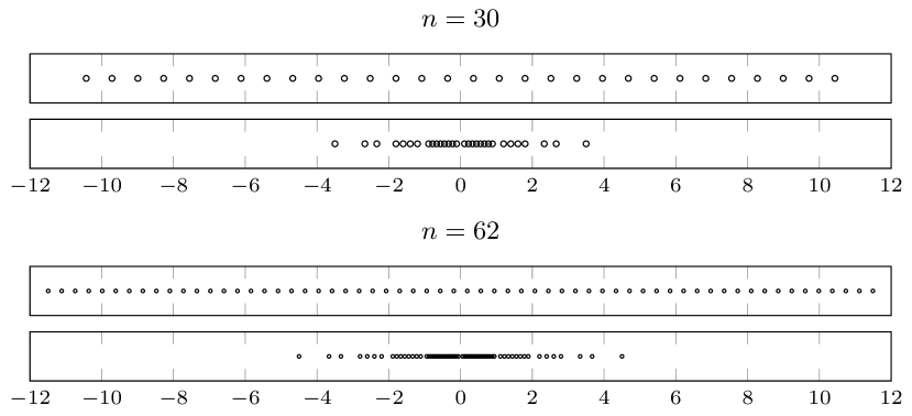
Figure 1: Comparison of the evaluation points used by the algorithms $A^{\dagger}_{n}$ and $A^{*}_{n}$ from Sections 2 and 3, respectively, for $n=30$ and $n=62$. The uniform points used by $A^{\dagger}_{n}$ in (2.1), with $T$ given in (2.10) for $\alpha=4$, $q=2$, $p=1$ and $\varepsilon=0.25$, are displayed in the top panels. The bottom panels display one possible set of points that can be used to construct the algorithm $A^{*}_{n}$ of Corollary 3.5. The density of these points decreases exponentially fast when moving away from the origin. The algorithm $A^{*}_{n}$ converges with the optimal rate $n^{-\alpha}$, while the rate of convergence of $A^{\dagger}_{n}$ is optimal up to a logarithmic factor.

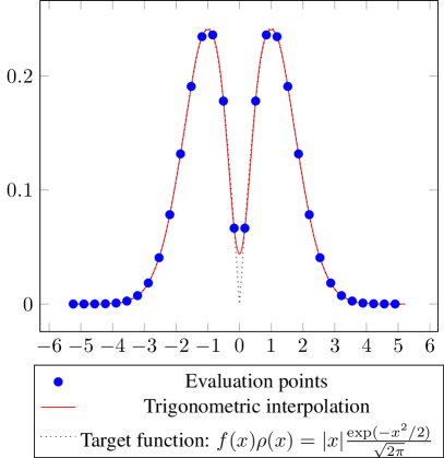
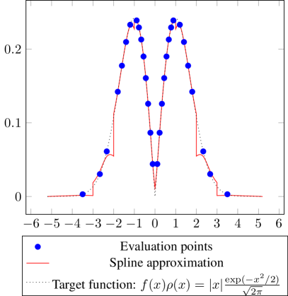
Figure 2: A comparison of trigonometric interpolation from Section 2 and spline approximation from Section 3 when $f(x)=\lvert x\rvert$, $p=1$ and $q=2$. We plot the weighted approximations $\rho A^{\dagger}_{n}(f)$ with $n=31$ and $\varepsilon=0.25$ (left) and $\rho A^{*}_{n}(f)$ with $n=30$ (right). The spline approximation has been constructed using a Matérn kernel of order $\gamma=3/2$ [see (3.6)], which is a reproducing kernel for a Sobolev space of order two. Observe how the spline approximation is more accurate close to the origin than the trigonometric interpolant.

2 Trigonometric interpolation

This section introduces our first algorithm based on trigonometric interpolation and analyses its $L^{p}_{\rho}$-error in terms of the number of function evaluation $n$. The algorithm is denoted by $A^{\dagger}_{n}:W^{\alpha,q}_{\rho}\to L^{p}_{\rho}$.

Definition 2.1 (Trigonometric interpolation with cutoff $A^{\dagger}_{n}$).

Let $g\coloneqq f\rho^{1/p}$. We define the approximation algorithm

$$A^{\dagger}_{n}(f)\coloneqq\rho^{-1/p}\mathcal{I}_{n}(f\rho^{1/p})=\rho^{-1/p}\mathcal{I}_{n}(g),$$ (2.1)

with $\mathcal{I}_{n}$ being the trigonometric interpolation on $[-T,T]$:

$$\mathcal{I}_{n}(g)\coloneqq\begin{cases}\sum_{k=-\lfloor n/2\rfloor}^{\lfloor n/2\rfloor}\widehat{g}_{a}(k)\phi_{k}^{[-T,T]}(x)&\text{if $x\in[-T,T],$}\\ 0&\text{otherwise,}\end{cases}$$

where $\phi_{k}^{[-T,T]}(x)\coloneqq\exp(2\pi ik(x+T)/(2T))/\sqrt{2T}$ are orthonormal Fourier basis on $L^{2}([-T,T])$. The coefficients $\widehat{g}_{a}(k)$ are calculated using equidistant points as

$$\widehat{g}_{a}(k)\coloneqq\frac{1}{n}\sum_{j=0}^{n-1}g(\xi_{j})\overline{\phi_{k}^{[-T,T]}}(\xi_{j}),\quad\text{ with }\quad\xi_{j}\coloneqq\frac{2T}{n}j-T,\ j=0,\dots,n-1.$$

We will bound the $L^{p}_{\rho}$ error of the above algorithm by decomposing it into two parts:

$$\begin{split}\|f-A^{\dagger}_{n}(f)\|_{L_{\rho}^{p}}\leq{}&\left(\int_{\mathbb{R}\setminus[-T,T]}\left|f(x)-[A^{\dagger}_{n}(f)](x)\right|^{p}\rho(x)\,\mathrm{d}x\right)^{1/p}\\ &+\left(\int_{-T}^{T}\left|f(x)-[A^{\dagger}_{n}(f)](x)\right|^{p}\rho(x)\,\mathrm{d}x\right)^{1/p}.\end{split}$$ (2.2)

For the first term, since we have $A^{\dagger}_{n}(f)=0$ outside the interval $[-T,T]$, we simply bound $(\int_{\mathbb{R}\setminus[-T,T]}|f(x)|^{p}\rho(x)\,\mathrm{d}x)^{1/p}$ using the decay of $g=f\rho^{1/p}$. In the following lemma, we obtain this decay of $g$ and its derivatives.

Lemma 2.2 (Decay of the function $g=f\rho^{1/p}$).

Let $1\leq p<q<\infty$, $\alpha\in\mathbb{N}$ and $f\in W^{\alpha,q}_{\rho}$. Then for arbitrary $\varepsilon\in(0,\frac{q-p}{pq})$ and $g=f\rho^{1/p}$, the following quantity is bounded:

$$\|g\|_{\textup{decay}}\coloneqq\sup_{\begin{subarray}{c}x\in\mathbb{R}\\ \tau\in\{0,\ldots,\alpha-1\}\end{subarray}}\big{|}\rho^{1/q-1/p+\varepsilon}(x)g^{(\tau)}(x)\big{|}<\infty.$$

Proof.

First we note that $1/q-1/p+\varepsilon<0$. In the following, we use the Sobolev inequality for $F_{\tau}(x)\coloneqq\rho^{1/q-1/p+\varepsilon}(x)g^{(\tau)}(x)$. That is, from the boundedness of $\|F_{\tau}\|_{L^{1}(\mathbb{R})}$ and $\|F_{\tau}^{\prime}\|_{L^{1}(\mathbb{R})}$ we deduce the boundedness of $\|F_{\tau}\|_{L^{\infty}(\mathbb{R})}$. Let $H_{\ell}(x)$ be the $\ell$-th degree probabilists’ Hermite polynomial,

$$H_{\ell}(x)=\frac{(-1)^{\ell}}{\sqrt{\ell!}}\mathrm{e}^{x^{2}/2}\frac{\,\mathrm{d}^{\ell}}{\,\mathrm{d}x^{\ell}}\mathrm{e}^{-x^{2}/2}.$$

First notice from the definition of Hermite polynomial that

$$\frac{\mathrm{d}^{\ell}}{\mathrm{d}x^{\ell}}\rho(x)^{1/p}=p^{-\ell/2}(-1)^{\ell}{\sqrt{\ell!}}H_{\ell}\left(\frac{x}{\sqrt{p}}\right)\rho(x)^{1/p}.$$

Hence, for $\tau=0,\ldots,\alpha-1,$ by applying the chain rule to $g^{(\tau)}$ we have

$$\|F_{\tau}(x)\|_{L^{1}(\mathbb{R})} \leq\sum_{\ell=0}^{\tau}\binom{\tau}{\ell}\|p^{-\ell/2}(-1)^{\ell}{\sqrt{\ell!}}H_{\ell}\left(\frac{x}{\sqrt{p}}\right)\rho(x)^{1/p}\rho^{1/q-1/p+\varepsilon}(x)f^{(\tau-\ell)}(x)\|_{L^{1}(\mathbb{R})}$$

$$\leq\sum_{\ell=0}^{\tau}\binom{\tau}{\ell}{\sqrt{\ell!}}p^{-\ell/2}\|H_{\ell}\left(\frac{x}{\sqrt{p}}\right)\rho(x)^{1/p}\rho^{1/q-1/p+\varepsilon}(x)f^{(\tau-\ell)}(x)\|_{L^{1}(\mathbb{R})}$$

$$\leq\sum_{\ell=0}^{\tau}\binom{\tau}{\ell}{\sqrt{\ell!}}p^{-\ell/2}\sup_{x\in\mathbb{R}}\left|H_{\ell}\left(\frac{x}{\sqrt{p}}\right)\rho^{\varepsilon}(x)\right|\left(\int_{\mathbb{R}}|f^{(\tau-\ell)}(x)|^{q}\rho(x)\,\mathrm{d}x\right)^{1/q}$$

$$=\sum_{\ell=0}^{\tau}\binom{\tau}{\ell}{\sqrt{\ell!}}p^{-\ell/2}\sup_{x\in\mathbb{R}}\left|H_{\ell}\left(\frac{x}{\sqrt{p}}\right)\rho^{\varepsilon}(x)\right|\|f^{(\tau-\ell)}(x)\|_{L^{q}_{\rho}}<\infty,$$

where in the last line, $\|f^{(\tau-\ell)}(x)\|_{L^{q}_{\rho}}$ is bounded because $f\in W^{\alpha,q}_{\rho}$, and the supremum term is also bounded because $H_{\ell}$ has at most only polynomial growth. At the same time, we have

$$\|F_{\tau}^{\prime}\|_{L^{1}(\mathbb{R})}\leq{} \|\rho^{1/q-1/p+\varepsilon}(x)g^{(\tau+1)}\|_{L^{1}(\mathbb{R})}+\|(1/p-1/q-\varepsilon)x\rho^{1/q-1/p+\varepsilon}(x)g^{(\tau)}\|_{L^{1}(\mathbb{R})}$$

$$\leq{} \sum_{\ell=0}^{\tau+1}\binom{\tau+1}{\ell}{\sqrt{\ell!}}p^{-\ell/2}\sup_{x\in\mathbb{R}}\left|H_{\ell}\left(\frac{x}{\sqrt{p}}\right)\rho^{\varepsilon}(x)\right|\|f^{(\tau-\ell+1)}(x)\|_{L^{q}_{\rho}}$$

$$+\sum_{\ell=0}^{\tau}\binom{\tau}{\ell}{\sqrt{\ell!}}p^{-\ell/2}\sup_{x\in\mathbb{R}}\left|H_{\ell}\left(\frac{x}{\sqrt{p}}\right)\rho^{\varepsilon}(x)\right|\|f^{(\tau-\ell)}(x)\|_{L^{q}_{\rho}}<\infty.$$

Thus we have $\|g\|_{\textup{decay}}<\infty$. ∎

For the second term in (2.2), we introduce a suitable auxiliary function $G$ and consider the bound

$$\bigg{(}\int_{-T}^{T}|f(x)-[A^{\dagger}_{n}(f)](x)|^{p}\rho(x)\,\mathrm{d}x\bigg{)}^{1/p}={} \bigg{(}\int_{-T}^{T}|g(x)-[\mathcal{I}_{n}(g)](x)|^{p}\,\mathrm{d}x\bigg{)}^{1/p}$$

$$={} \|g-\mathcal{I}_{n}(g)\|_{L^{p}([-T,T])}$$

$$\begin{split}\leq{}&\|g-G\|_{L^{p}([-T,T])}+\|G-\mathcal{I}_{n}(G)\|_{L^{p}([-T,T])}\\ &+\|\mathcal{I}_{n}(G)-\mathcal{I}_{n}(g)\|_{L^{p}([-T,T])}.\end{split}$$ (2.3)

Lemma 2.7 will upper bound the three terms in (2.3). For that, we need the following Lemmas 2.3 to 2.6.

Lemma 2.3 (Auxiliary periodic function and its properties).

Let $1\leq p<q<\infty$, $\alpha\in\mathbb{N}$ and $T>0$. For $f\in W^{\alpha,q}_{\rho}$, let $g=f\rho^{1/p}$ and define $G:[-T-d,T+d]\to\mathbb{R}$ by

$$G(x)\coloneqq g(x)-\sum_{\tau=1}^{\alpha}\frac{B^{[-T,T]}_{\tau}(x)}{\tau!}\left(\int_{-T}^{T}g^{(\tau)}(y)\,\mathrm{d}y\right),$$ (2.4)

with an arbitrarily small $d>0$, where $B^{[-T,T]}_{\tau}$ denotes the scaled Bernoulli polynomial of degree $\tau$ on $[-T,T]$, i.e.,

$$B^{[-T,T]}_{\tau}(x)=(2T)^{\tau-1}B_{\tau}\left(\frac{x+T}{2T}\right)$$

with $B_{\tau}$ being the standard Bernoulli polynomial of degree $\tau$. Then, the auxiliary function $G$ is $(\alpha-1)$-times continuously differentiable with $G^{(\alpha-1)}$ being absolutely continuous on $[-T,T]$, and satisfies $G^{(\tau)}(-T)=G^{(\tau)}(T)$ for all $\tau=0,\ldots,\alpha-1$. Furthermore, the auxiliary function $G$ has its $\alpha$-th weak derivative $G^{(\alpha)}$ in $L^{q}([-T,T])$ which can be identified as a function over a $2T$-periodic torus $\mathbb{T}([-T,T))$ with

$$\int_{\mathbb{T}([-T,T))}|G^{(\alpha)}(x)|^{q}\,\mathrm{d}x<\infty.$$

Proof.

The proof is similar to [10, Lemma 4.1], where the case with $p=1$ and $q=2$ was proved. Recall that for $\tau,\tau^{\prime}\in\mathbb{N}_{0}$ scaled Bernoulli polynomials satisfy

$$\frac{\mathrm{d}^{\tau^{\prime}}}{\mathrm{d}x^{\tau^{\prime}}}\frac{B^{[-T,T]}_{\tau}(x)}{\tau!}=\left\{\begin{array}[]{ll}0&\text{ if }\tau^{\prime}>\tau,\\ \frac{B^{[-T,T]}_{\tau-\tau^{\prime}}(x)}{\left(\tau-\tau^{\prime}\right)!}&\text{ if }\tau^{\prime}\leq\tau\end{array}\right.$$

and

$$\int_{-T}^{T}B_{\tau}^{[-T,T]}(x)\,\mathrm{d}x=\left\{\begin{array}[]{ll}1&\text{ if }\tau=0,\\ 0&\text{ if }\tau\neq 0.\end{array}\right.$$

From these properties we have

$$\int_{-T}^{T}G^{(\tau)}(x)\,\mathrm{d}x=\int_{-T}^{T}g^{(\tau)}(x)\,\mathrm{d}x-\left(\int_{-T}^{T}B^{[-T,T]}_{0}(x)\,\mathrm{d}x\right)\left(\int_{-T}^{T}g^{(\tau)}(s)\,\mathrm{d}s\right)=0,$$

for $\tau=1,\ldots,\alpha$. Since $f\in W^{\alpha,q}_{\rho}$, $g^{(\tau)}$ and $G^{(\tau)}$ are absolutely continuous on $(-T-d,T+d)$ for $\tau=0,1,\ldots,\alpha-1$. By using the fundamental theorem of calculus, we now obtain

$$G^{(\tau)}(-T)=G^{(\tau)}(T)\quad\text{for }\ \tau=0,\ldots,\alpha-1.$$ (2.5)

Next, we note that $G^{(\alpha)}$ and $g^{(\alpha)}$ only differ by the constant $\frac{1}{2T}\int_{-T}^{T}g^{(\alpha)}(y)\,\mathrm{d}y$ on $[-T,T]$. Since $f^{(\alpha)}\in L^{q}_{\rho}$, we know $g^{(\alpha)}$ is in $L^{q}([-T,T])$. Due to matching boundary values $G^{(\alpha-1)}(-T)=G^{(\alpha-1)}(T)$ and absolute continuity of $G^{(\alpha-1)}$ on $(-T-\delta,T+\delta)$, we have $\|G^{(\alpha)}\|_{L^{p}(\mathbb{T}([-T,T]))}<\infty$. ∎

Lemma 2.4 (Norm estimate on bounded intervals).

Let $1\leq p<q<\infty$, $\alpha\in\mathbb{N}$, $a<b$ and $\varepsilon\in[0,q-p)$. Then

$$\|g\|_{W^{\alpha,q}([a,b])}\leq C_{p,q,\alpha,\varepsilon}\,\rho^{\varepsilon/p}(c)\|f\|_{W^{\alpha,q}_{\rho}},$$

where $c=\min_{x\in[a,b]}\lvert x\rvert$.

Proof.

We have

$$\|g\|_{W^{\alpha,q}([a,b])} =\left(\sum_{\tau=0}^{\alpha}\int_{a}^{b}\lvert g^{(\tau)}(x)\rvert^{q}\,\mathrm{d}x\right)^{1/q}$$

$$=\left(\sum_{\tau=0}^{\alpha}\int_{a}^{b}\lvert(f\rho^{1/p}))^{(\tau)}(x)\rvert^{q}\,\mathrm{d}x\right)^{1/q}$$

$$\leq\sum_{\tau=0}^{\alpha}\left(\int_{a}^{b}\bigg{\lvert}\sum_{\ell=0}^{\tau}\binom{\tau}{\ell}f^{(\tau-\ell)}(x)p^{-\ell/2}H_{\ell}\bigg{(}\frac{x}{\sqrt{p}}\bigg{)}\rho^{1/p}(x)\bigg{\rvert}^{q}\,\mathrm{d}x\right)^{1/q}$$

$$\leq\sum_{\tau=0}^{\alpha}\sum_{\ell=0}^{\tau}\binom{\tau}{\ell}\left(\int_{a}^{b}\bigg{\lvert}f^{(\tau-\ell)}(x)p^{-\ell/2}H_{\ell}\bigg{(}\frac{x}{\sqrt{p}}\bigg{)}\rho^{1/p}(x)\bigg{\rvert}^{q}\,\mathrm{d}x\right)^{1/q}$$

$$\leq\sum_{\tau=0}^{\alpha}\sum_{\ell=0}^{\tau}\binom{\tau}{\ell}\sup_{x\in[a,b]}\bigg{\lvert}p^{-\ell/2}H_{\ell}\bigg{(}\frac{x}{\sqrt{p}}\bigg{)}\rho^{(q-p)/p}(x)\bigg{\rvert}\left(\int_{a}^{b}\lvert f^{(\tau-\ell)}(x)\rvert^{q}\rho(x)\,\mathrm{d}x\right)^{1/q}$$

$$\kern-19.91692pt\leq\sum_{\tau=0}^{\alpha}\sum_{\ell=0}^{\tau}\binom{\tau}{\ell}\sup_{x\in[a,b]}\bigg{\lvert}p^{-\ell/2}H_{\ell}\bigg{(}\frac{x}{\sqrt{p}}\bigg{)}\rho^{(q-p-\varepsilon)/p}(x)\bigg{\rvert}\rho^{\varepsilon/p}(c)\left(\int_{a}^{b}\lvert f^{(\tau-\ell)}(x)\rvert^{q}\rho(x)\,\mathrm{d}x\right)^{1/q}$$

$$\leq C_{p,q,\alpha,\varepsilon}\,\rho^{\varepsilon/p}(c)\|f\|_{W^{\alpha,q}_{\rho}},$$

where we used the facts that $H_{\ell}(\cdot/\sqrt{p})\rho^{(q-p-\varepsilon)/p}$ is bounded on the real line and that $\rho(x)$ is decreasing in $\lvert x\rvert$. ∎

For obtaining trigonometric interpolation error on $[-T,T]$, we make use of results from trigonometric interpolation on $[0,2\pi]$. For that sake, we need the following estimate for the effect of linear scaling $S_{T}:[0,2\pi]\to[-T,T]$ given by $S_{T}(x)\coloneqq Tx/\pi-T$.

Lemma 2.5 (Boundedness of $\|g\circ S_{T}\|_{W^{\alpha,q}([0,2\pi])}$).

Let $1\leq p<q<\infty$, $\alpha\in\mathbb{N}$, and $f\in W^{\alpha,q}_{\rho}$. For $g=f\rho^{1/p}$ we define $h\coloneqq g\circ S_{T}$. Then, for $T\geq 1$ we have

$$\|h\|_{W^{\alpha,q}([0,2\pi])}\leq C_{p,q,\alpha}T^{\alpha-1/q}\|f\|_{W^{\alpha,q}_{\rho}}.$$

Proof.

We have

$$\|h\|_{W^{\alpha,q}([0,2\pi])}=\left(\sum_{\tau=0}^{\alpha}\int_{0}^{2\pi}\lvert h^{(\tau)}(x)\rvert^{q}\,\mathrm{d}x\right)^{1/q} =\left(\sum_{\tau=0}^{\alpha}\int_{0}^{2\pi}\lvert(g\circ S_{T})^{(\tau)}(x)\rvert^{q}\,\mathrm{d}x\right)^{1/q}$$

$$=\left(\sum_{\tau=0}^{\alpha}\int_{0}^{2\pi}\lvert(T/\pi)^{\tau}(g^{(\tau)}\circ S_{T})(x)\rvert^{q}\,\mathrm{d}x\right)^{1/q}$$

$$=\left(\sum_{\tau=0}^{\alpha}(T/\pi)^{(\tau-1)q}\int_{-T}^{T}\lvert g^{(\tau)}(x)\rvert^{q}\,\mathrm{d}x\right)^{1/q}$$

$$\leq C_{q,\alpha}T^{\alpha-1/q}\lVert g\rVert_{W^{\alpha,q}([-T,T])}.$$

The claim then follows from Lemma 2.4 with $a=-T$, $b=T$, and $\varepsilon=0$. ∎

Lemma 2.6 ($L^{p}$ interpolation error for periodic functions).

Let $1\leq p<q<\infty$, $\alpha\in\mathbb{N}$, and $f\in W^{\alpha,q}_{\rho}$. Define $g=f\rho^{1/p}$ and an auxiliary periodic function $G$ as in (2.4). Then

$$\|G-\mathcal{I}_{n}(G)\|_{L^{p}([-T,T])}\leq C_{p,q,\alpha}T^{\alpha-1/q+1/p}\|f\|_{W^{\alpha,q}_{\rho}}\frac{1}{n^{\alpha}}.$$

Proof.

The result by Temlyakov [30, Theorem 2.4.4], where the interpolation operator is denoted by $I_{m}$, applies to our setting. Therein, the function space considered is defined via convolution kernels, but the norm equivalence to periodic Sobolev spaces

$$W^{\alpha,q}(\mathbb{T}[0,2\pi))\coloneqq\big{\{}f\;\big{|}\;f\in W^{\alpha,q}([0,2\pi]),f^{(\tau)}(0)=f^{(\tau)}(2\pi)\;\text{for}\;\tau=0,\ldots,\alpha-1\big{\}}$$

is shown in [32, Theorem 2.7]. Hence, by letting $S_{T}(x)\coloneqq Tx/\pi-T$, [30, Theorem 2.4.4] leads to

$$\|G\circ S_{T}-\mathcal{I}_{n}(G\circ S_{T})\|_{W^{\alpha,q}(\mathbb{T}(0,2\pi))}\leq C^{\prime}_{p,q,\alpha}\|G\circ S_{T}\|_{W^{\alpha,q}(\mathbb{T}(0,2\pi))}\frac{1}{n^{\alpha}}.$$

Further, by Lemma 2.5, the above error is bounded by

$$\leq C^{\prime\prime}_{p,q,\alpha}T^{\alpha-1/q}\|f\|_{W^{\alpha,q}_{\rho}}\frac{1}{n^{\alpha}}.$$

At the same time, since $S_{T}$ is a plain linear scaling, we have

$$\|G\circ S_{T}-\mathcal{I}_{n}(G\circ S_{T})\|_{L^{p}(\mathbb{T}(0,2\pi))}=\left(\frac{\pi}{T}\right)^{1/p}\|G-\mathcal{I}_{n}(G)\|_{L^{p}(\mathbb{T}(-T,T))}.$$

Thus we have proved the claim. ∎

Lemma 2.7 (Error bound on $[-T,T]$ for $A^{\dagger}_{n}$).

Let $1\leq p<q<\infty$, $\alpha\in\mathbb{N}$, and $f\in W^{\alpha,q}_{\rho}$. Choose $\varepsilon\in(0,\frac{q-p}{pq})$ arbitrarily. Then the approximation error on $[-T,T]$ by the algorithm $A^{\dagger}_{n}$ is bounded by

$$\|f-A^{\dagger}_{n}(f)\|_{L_{\rho}^{p}([-T,T])} =\left(\int_{-T}^{T}\left|f(x)\rho^{1/p}(x)-\mathcal{I}_{n}(f\rho^{1/p})\right|^{p}\,\mathrm{d}x\right)^{1/p}$$

$$\leq C_{1}T^{\alpha-1/q+1/p}n^{-\alpha}+C_{2}(\ln n)\max\{1,(2T)^{\alpha-1+1/p}\}\mathrm{e}^{-\frac{(q-p)/pq-\varepsilon}{2}T^{2}},$$

where the constants $C_{1}$ and $C_{2}$ do not depend on $n$ or $T$.

Proof.

From Lemma 2.2, we know that for $g\coloneqq f\rho^{1/p}$ the quantity

$$\|g\|_{\text{decay}}=\sup_{\begin{subarray}{c}x\in\mathbb{R}\\ \tau\in\{0,\ldots,\alpha-1\}\end{subarray}}\left|\rho^{1/q-1/p+\varepsilon}(x)g^{(\tau)}(x)\right|$$

is bounded. As mentioned above, we consider the following bound:

$$\|f-A^{\dagger}_{n}(f)\|_{L_{\rho}^{p}([-T,T])} =\|g-\mathcal{I}_{n}{g}\|_{L^{p}([-T,T])}$$

$$\kern-56.9055pt\leq\|g-G\|_{L^{p}([-T,T])}+\|G-\mathcal{I}_{n}(G)\|_{L^{p}([-T,T])}+\|\mathcal{I}_{n}(G)-\mathcal{I}_{n}(g)\|_{L^{p}([-T,T])}.$$ (2.6)

For the first term in the last line of (2.6), we have

$$\|g-G\|_{L^{p}([-T,T])} \leq\sum_{\tau=1}^{\alpha}\frac{\|B^{[-T,T]}_{\tau}(x)\|_{L^{p}([-T,T])}}{\tau!}\left|\int_{-T}^{T}g^{(\tau)}(s)\,\mathrm{d}s\right|$$

$$\leq\sum_{\tau=1}^{\alpha}\frac{\|B^{[-T,T]}_{\tau}(x)\|_{L^{\infty}([-T,T])}\;(2T)^{1/p}}{\tau!}\left|\int_{-T}^{T}g^{(\tau)}(s)\,\mathrm{d}s\right|$$

$$\leq\sum_{\tau=1}^{\alpha}(2T)^{\tau-1+1/p}\left|\int_{-T}^{T}g^{(\tau)}(s)\,\mathrm{d}s\right|$$

$$\leq\alpha\max\{1,(2T)^{\alpha-1+1/p}\}\|g\|_{\text{decay}}\;C_{p,q,\varepsilon}\;\mathrm{e}^{-\frac{(q-p)/pq-\varepsilon}{2}T^{2}},$$ (2.7)

where in the penultimate line, we used $|\frac{B^{[-T,T]}_{\tau}(x)}{\tau!}|\leq\frac{(2T)^{\tau-1}}{2}$ for $x\in[-T,T]$; see [23, Equation (6)] or [14].

We proceed to the third term. We have

$$\|\mathcal{I}_{n} (g-G)\|_{L^{p}([-T,T])}$$

$$\leq\|\mathcal{I}_{n}\|_{C([-T,T])\to L^{p}([-T,T])}\|g-G\|_{L^{p}([-T,T])}$$

$$\leq\|\mathcal{I}_{n}\|_{C([-T,T])\to L^{p}([-T,T])}\alpha\max\{1,(2T)^{\alpha-1+1/p}\}\;\|g\|_{\text{decay}}\;C_{p,q,\varepsilon}\;\mathrm{e}^{-\frac{(q-p)/pq-\varepsilon}{2}T^{2}}.$$ (2.8)

Now the operator norm of the interpolation, from continuous functions to $L^{p}$, can be bounded using the Lebesgue constant $\Lambda_{n}$ for trigonometric interpolation by

$$\|\mathcal{I}_{n}\|_{C([-T,T])\to L^{p}([-T,T])}\leq 2T\Lambda_{n}\leq 2T\left(\frac{\pi+4}{\pi}+\frac{2\ln n}{\pi}\right),$$

where this explicit constant here can be found, e.g., in [26, Theorem 2.1], or we refer to [5] as an earlier result.

For the second term in (2.6), we know from Lemma 2.6 that

$$\|G-\mathcal{I}_{n}(G)\|_{L^{p}([-T,T])}\leq C_{p,q,\alpha}T^{\alpha-1/q+1/p}\|f\|_{W^{\alpha,q}_{\rho}}\frac{1}{n^{\alpha}}.$$ (2.9)

Summing up all three terms, (2),(2), and (2.9), we obtain the error bound

$$\|f-A^{\dagger}_{n}(f)\|_{L_{\rho}^{p}([-T,T])}\leq C_{1}T^{\alpha-1/q+1/p}n^{-\alpha}+C_{2}(\ln n)\max\{1,(2T)^{\alpha-1+1/p}\}\mathrm{e}^{-\frac{(q-p)/pq-\varepsilon}{2}T^{2}}.$$

∎

Lemma 2.8 (Error bound on tails).

Let $1\leq p<q<\infty$, $\alpha\in\mathbb{N}$, and $f\in W^{\alpha,q}_{\rho}$. Set $g=f\rho^{1/p}$. Choose $\varepsilon\in(0,\frac{q-p}{pq})$ arbitrarily. For the error outside the interval $[-T,T]$, we have

$$\left(\int_{\mathbb{R}\setminus[-T,T]}\left|f(x)\right|^{p}\rho(x)\,\mathrm{d}x\right)^{1/p} \leq C_{p,q,\varepsilon}\;\|g\|_{\textup{decay}}\;T^{-1/p}\;\mathrm{e}^{-\frac{(q-p)/pq-\varepsilon}{2}T^{2}}.$$

Proof.

Let $r\coloneqq 1/p-1/q-\varepsilon>0$. Using Lemma 2.2 we have

$$\left(\int_{\mathbb{R}\setminus[-T,T]}\left|g(x)\right|^{p}\,\mathrm{d}x\right)^{1/p} \leq\left(\int_{\mathbb{R}\setminus[-T,T]}\left(\|g\|_{\text{decay}}\frac{\mathrm{e}^{-rx^{2}/2}}{\sqrt{2\pi}^{r}}\right)^{p}\,\mathrm{d}x\right)^{1/p}$$

$$\leq\|g\|_{\text{decay}}\left(\frac{2}{T}\int_{T}^{\infty}\frac{x\mathrm{e}^{-rpx^{2}/2}}{\sqrt{2\pi}^{rp}}\,\mathrm{d}x\right)^{1/p}$$

$$=\|g\|_{\text{decay}}\left(\frac{2}{rpT\sqrt{2\pi}^{rp}}\;\mathrm{e}^{-rpT^{2}/2}\right)^{1/p}=\frac{2^{1/p}}{(rpT)^{1/p}\sqrt{2\pi}^{r}}\;\mathrm{e}^{-rT^{2}/2}.$$

∎

Theorem 2.9 (Error bound on $\mathbb{R}$ for $A^{\dagger}_{n}$).

Let $1\leq p<q<\infty$, $\alpha\in\mathbb{N}$, and $f\in W^{\alpha,q}_{\rho}$. Choose $\varepsilon\in(0,\frac{q-p}{pq})$ arbitrarily. Set the cut-off interval $[-T,T]$ with

$$T=\sqrt{2\alpha\left(\frac{q-p}{pq}-\varepsilon\right)^{-1}\ln n}.$$ (2.10)

Then, for any integer $n\geq 2$, the approximation error on $\mathbb{R}$ by the algorithm $A^{\dagger}_{n}$ is bounded by

$$\|f-A^{\dagger}_{n}(f)\|_{L_{\rho}^{p}} =\left(\int_{\mathbb{R}}\left|g(x)\rho^{1/p}(x)-\mathcal{I}_{n}(g\rho^{1/p})\right|^{p}\,\mathrm{d}x\right)^{1/p}\leq C\frac{(\ln n)^{\frac{\alpha}{2}+\frac{1}{2}+\frac{1}{2p}}}{n^{\alpha}}.$$

Proof.

We consider the error bound (2.2). With our choice of the cutoff interval, Lemma 2.7 tells us that

$$\left(\int_{-T}^{T}\left|f(x)-[A^{\dagger}_{n}(f)](x)\right|^{p}\rho(x)\,\mathrm{d}x\right)^{1/p}\leq C_{1}(\ln n)^{\frac{\alpha}{2}-\frac{1}{2q}+\frac{1}{2p}}n^{-\alpha}+C_{2}(\ln n)^{\frac{\alpha}{2}+\frac{1}{2}+\frac{1}{2p}}n^{-\alpha},$$

here we used the fact that $T$ is always bigger than $1$ for $n\geq 2$, since $0<\frac{q-p}{pq}-\varepsilon<1$. For the error outside the interval, using Lemma 2.8, we obtain

$$\left(\int_{\mathbb{R}\setminus[-T,T]}\left|f(x)\right|^{p}\rho(x)\,\mathrm{d}x\right)^{1/p}\leq C_{p,q,\varepsilon}\;\|g\|_{\text{decay}}\;\mathrm{e}^{-\frac{(q-p)/pq-\varepsilon}{2}T^{2}}=C_{p,q,\varepsilon}\;\|g\|_{\text{decay}}\;n^{-\alpha}.$$

Therefore, the total error is bounded by

$$\|f-A^{\dagger}_{n}(f)\|_{L_{\rho}^{p}}\leq C(\ln n)^{\frac{\alpha}{2}+\frac{1}{2}+\frac{1}{2p}}n^{-\alpha}.\qed$$

Remark 2.10 (Periodic auxiliary function $G$).

This proof strategy of introducing the auxiliary function $G$ can be applied to other algorithms or problems. Let us elaborate this part here. Consider an abstract problem of approximating a linear operator or a linear functional $S:\mathcal{H}_{1}\to\mathcal{H}_{2}$ by a linear algorithm $A_{n}:\mathcal{H}_{1}\to\mathcal{H}_{2}$. This is a typical setting in information-based complexity, see, e.g., [22, Section 4.4]. Then, the error has the following upper bound for any $g\in\mathcal{H}_{1}$:

$$\|S(g)-A_{n}(g)\|_{\mathcal{H}_{2}} \leq\|S(g)-S(G)\|_{\mathcal{H}_{2}}+\|S(G)-A_{n}(G)\|_{\mathcal{H}_{2}}+\|A_{n}(G)-A_{n}(g)\|_{\mathcal{H}_{2}}$$

$$=\|S(g-G)\|_{\mathcal{H}_{2}}+\|S(G)-A_{n}(G)\|_{\mathcal{H}_{2}}+\|A_{n}(G-g)\|_{\mathcal{H}_{2}}.$$ (2.11)

This strategy is first used in [23] for a multivariate integration problem in which $S(g)=\int_{\mathbb{R}^{d}}g({\boldsymbol{x}})\,\mathrm{d}{\boldsymbol{x}}$ and $A_{n}$ is a specific quadrature rule, called a scaled rank-$1$ lattice rule. Therein, the first error term in (2.10), $\|S(g-G)\|_{\mathcal{H}_{2}}$, happens to vanish due to properties of the integration functional. However, as we have seen, this term can be bounded just like the third term $\|A_{n}(G-g)\|_{\mathcal{H}_{2}}$ for general linear algorithms.

In Theorem 2.9, the choice of the cut-off parameter $T$ depends on the smoothness $\alpha$ of the approximand function. However, this information may not be available in practice. Following [10, Corollary 4.4] and [7, Remark 3.11], one can replace $\alpha$ by a slowly increasing function $\gamma(n)$ such as $\max(\ln(\ln n),0)$, and still achieve the convergence rate $n^{-\alpha}$, up to a factor $(\gamma(n)\ln n)^{\frac{\alpha}{2}+\frac{1}{2}+\frac{1}{2p}}$.

Corollary 2.11 ($\alpha$-free construction).

Let assumptions of Theorem 2.9 be satisfied. Choose $\varepsilon\in(0,\frac{q-p}{pq})$ arbitrarily. Choose a non-decreasing function $\gamma(n):\mathbb{N}\to\mathbb{R}$ satisfying $\lim_{n\to\infty}\gamma(n)=\infty$, and set the cut-off interval $[-T,T]$ with

$$T=\sqrt{2\gamma(n)\left(\frac{q-p}{pq}-\varepsilon\right)^{-1}\ln n}.$$

Then, for any integer $n\geq\gamma^{-1}(\alpha)\coloneqq\min\{m\in\mathbb{N}\mid\gamma(m)\geq\alpha\}$, the approximation error on $\mathbb{R}$ by the algorithm $A^{\dagger}_{n}$ is bounded by

$$\|f-A^{\dagger}_{n}(f)\|_{L_{\rho}^{p}} =\left(\int_{\mathbb{R}}\left|g(x)\rho^{1/p}(x)-\mathcal{I}_{n}(g\rho^{1/p})\right|^{p}\,\mathrm{d}x\right)^{1/p}\leq C\frac{(\gamma(n)\ln n)^{\frac{\alpha}{2}+\frac{1}{2}+\frac{1}{2p}}}{n^{\alpha}}.$$

Remark 2.12 (Computational cost).

As mentioned in Introduction, the computational cost and memory usage of an FFT implementation of algorithm $A^{\dagger}_{n}$ are only $\mathcal{O}(n\log_{2}n)$ and $\mathcal{O}(n)$, respectively. The advantage of the method is mainly this cheap cost of construction. However, when the evaluation of the approximand function $f$ is much more expensive, one may wish to have the optimal convergence rate including the logarithmic factor, at the sacrifice of cheap construction. In such a case, we propose the optimal algorithm described in Section 3.

Remark 2.13 (Higher dimensions).

For multidimensional settings, where the dominating-mixed smoothness is considered (i.e., tensor product of one-dimensional Gaussian Sobolev spaces), it is possible to extend our algorithm in such a way that the construction cost is still $\mathcal{O}(n\log_{2}n)$. One possibility is using rank-$1$ lattices as interpolation nodes, e.g. [16, 18, 29, 28]. However, the convergence rate of approximation algorithms based on rank-$1$ lattice points deteriorates at least to $n^{-\alpha/2}$ for periodic functions [2], and thus unfortunately it is not possible to obtain the same rate $n^{-\alpha}$. Another possibility is the fast Smolyak construction [8] combined with our algorithm $A^{\dagger}_{n}$, which may attain the optimal rate up to a logarithmic factor.

3 Spline algorithms

In this section we consider a more refined decomposition of the real line. By partitioning the line into intervals of unit length and having the number of points placed within each interval decrease exponentially fast as one moves away from the origin, we construct an algorithm that attains the optimal rate $n^{-\alpha}$ in $W_{\rho}^{\alpha,q}$ when $q=2$. This construction is very similar to (and inspired by) those used in [4] and [9, Section 3].

3.1 Generic results

Let $W^{\alpha,q}(\mathbb{I})$ stand for the standard unweighted Sobolev space on an interval $\mathbb{I}$. That is, each element of this space is $\alpha$ times weakly differentiable on $\mathbb{I}$ and the weak derivatives are in $L^{q}(\mathbb{I})$. For each $\nu\in\mathbb{N}$, let $A_{\nu}^{\mathbb{I},1}\colon W^{\alpha,q}(\mathbb{I}_{1})\to L^{p}(\mathbb{I}_{1})$ be an approximation to $f\in W^{\alpha,q}(\mathbb{I}_{1})$ based on $\nu$ function values on the interval $\mathbb{I}_{1}=[0,1]$. We may interpret $A_{\nu}^{\mathbb{I},1}(f)$ as an element of $L^{p}(\mathbb{R})$ that vanishes on $\mathbb{R}\setminus\mathbb{I}_{1}$. We assume that there are positive constants $C_{0}$ and $\beta$ independent of $f$ or $\nu$ such that

$$\|f-A_{\nu}^{\mathbb{I},1}(f)\|_{L^{p}(\mathbb{I}_{1})}\leq C_{0}\nu^{-\beta}\|f\|_{W^{\alpha,q}(\mathbb{I}_{1})}$$ (3.1)

for all $f\in W^{\alpha,q}(\mathbb{I}_{1})$ and $\nu\in\mathbb{N}$. Let $\mathbb{I}_{k}=[k-1,k]$ for $k\geq 1$ and $\mathbb{I}_{k}=[-k,-k+1]$ for $k\leq-1$. By straightforward translation we obtain algorithms $A_{\nu}^{\mathbb{I},k}\colon W^{\alpha,q}(\mathbb{I}_{k})\to L^{p}(\mathbb{I}_{k})$ such that

$$\|f-A_{\nu}^{\mathbb{I},k}(f)\|_{L^{p}(\mathbb{I}_{k})}\leq C_{0}\nu^{-\beta}\|f\|_{W^{\alpha,q}(\mathbb{I}_{k})}$$ (3.2)

for all $f\in W^{\alpha,q}(\mathbb{I}_{k})$ and $\nu\in\mathbb{N}$. For $m\in\mathbb{N}$ and $\nu_{1},\ldots,\nu_{m}\in\mathbb{N}$ we set $n=2(\nu_{1}+\cdots+\nu_{m})$. Moreover, set $\nu_{-k}=\nu_{k}$. Define the algorithm $A^{*}_{n}\colon W^{\alpha,q}_{\rho}\to L^{p}_{\rho}$ that uses $n$ function values to approximate $f\in W^{\alpha,q}_{\rho}$ via

$$A^{*}_{n}(f)=\rho^{-1/p}\sum_{0<\lvert k\lvert\leq m}A_{\nu_{k}}^{\mathbb{I},k}(g_{k}),\quad\text{ where }g_{k}=f|_{\mathbb{I}_{k}}\rho^{1/p}.$$ (3.3)

Note that $A^{*}_{n}(f)$ vanishes on $\mathbb{R}\setminus[-m,m]$. We shall show that $A^{*}_{n}$ inherits the convergence rate (3.1) of $A_{\nu}^{\mathbb{I},1}$ if $m$ and $\nu_{1},\ldots,\nu_{m}$ are selected properly.

Proposition 3.1 (Generic error bound).

Let $1\leq p<q<\infty$, $\alpha\in\mathbb{N}$, and $f\in W^{\alpha,q}_{\rho}$. Then there are positive constants $C$ and $\delta$, which do not depend on $m$ or $\nu_{1},\ldots,\nu_{m}$, such that

$$\|f-A^{*}_{n}(f)\|_{L^{p}_{\rho}}\leq C\Bigg{(}\sum_{k=1}^{m}\mathrm{e}^{-\delta k^{2}}\nu_{k}^{-\beta}+\mathrm{e}^{-\delta m^{2}}\Bigg{)}.$$

Proof.

The proof is similar to those in Section 2. The error decomposes as

$$\|f-A^{*}_{n}(f)\|_{L^{p}_{\rho}}\leq\sum_{0<\lvert k\lvert\leq m}\|g_{k}-A_{\nu_{k}}^{\mathbb{I},k}(g_{k})\|_{L^{p}(\mathbb{I}_{k})}+\left(\int_{\mathbb{R}\setminus[-m,m]}\lvert f(x)\rvert^{p}\rho(x)\,\mathrm{d}x\right)^{1/p}.$$

Let $\varepsilon\in(0,\frac{q-p}{pq})$. Then Lemma 2.8 bounds the tail term as

$$\int_{\mathbb{R}\setminus[-m,m]}\lvert f(x)\rvert^{p}\rho(x)\,\mathrm{d}x=\int_{\mathbb{R}\setminus[-m,m]}\lvert g(x)\rvert^{p}\,\mathrm{d}x\leq C_{p,q,\varepsilon}\lVert g\rVert_{\textup{decay}}\,\mathrm{e}^{-\frac{(q-p)/pq-\varepsilon}{2}m^{2}},$$

where $g=f\rho^{1/p}$ and $\lVert g\rVert_{\textup{decay}}$ is finite by Lemma 2.2. The error bound (3.2) and Lemma 2.4 yield

$$\begin{split}\|g_{k}-A_{\nu_{k}}^{\mathbb{I},k}(g_{k})\|_{L^{p}(\mathbb{I}_{k})}&\leq C_{0}\nu_{k}^{-\beta}\lVert g_{k}\rVert_{W^{\alpha,q}(\mathbb{I}_{k})}\leq C_{0}C_{p,q,\alpha,\varepsilon}\,\rho^{\varepsilon/p}(\lvert k\rvert-1)\nu_{k}^{-\beta}\|f\|_{W^{\alpha,q}_{\rho}}.\end{split}$$

The above bound does not depend on the sign of $k$ because we require that $\nu_{-k}=\nu_{k}$. Hence there are positive constants $C$ and $\delta$ such that

$$\|f-A^{*}_{n}(f)\|_{L^{p}_{\rho}}\leq C\Bigg{(}\sum_{k=1}^{m}\mathrm{e}^{-\delta k^{2}}\nu_{k}^{-\beta}+\mathrm{e}^{-\delta m^{2}}\Bigg{)},$$

which completes the proof. ∎

Theorem 3.2 (Error bound for exponentially decaying points).

Let $1\leq p<q<\infty$, $\alpha\in\mathbb{N}$, and $m\in\mathbb{N}$. Set $\nu_{k}=2^{m-k}$ for $k=1,\ldots,m$. Then the algorithm $A^{*}_{n}$ defined in (3.3) uses $n=2(2^{m}-1)$ function values and satisfies

$$\|f-A^{*}_{n}(f)\|_{L^{p}_{\rho}}\leq Cn^{-\beta}$$

for any $f\in W_{\rho}^{\alpha,q}$, where the constant $C$ does not depend on $n$.

Proof.

The algorithm uses $n=2\sum_{k=1}^{m}\nu_{k}=2\sum_{k=1}^{m}2^{m-k}=2(2^{m}-1)$ function values. Proposition 3.1 yields

$$\|f-A^{*}_{n}(f)\|_{L^{p}_{\rho}}\leq C\Bigg{(}\sum_{k=1}^{m}\mathrm{e}^{-\delta k^{2}}\nu_{k}^{-\beta}+\mathrm{e}^{-\delta m^{2}}\Bigg{)}=C\Bigg{(}2^{-\beta m}\sum_{k=1}^{m}\mathrm{e}^{-\delta k^{2}}2^{\beta k}+\mathrm{e}^{-\delta m^{2}}\Bigg{)}.$$

Since $\sum_{k=1}^{\infty}\mathrm{e}^{-\delta k^{2}}2^{\beta k}<\infty$ and $\mathrm{e}^{-\delta m^{2}}$ decays faster than $2^{-\beta m}$ as $m\to\infty$, the claim follows from

$$2^{-\beta m}\leq(2^{m}-1)^{-\beta}=(n/2)^{-\beta}.\qed$$

To attain the optimal rate $n^{-\alpha}$ in $W_{\rho}^{\alpha,q}$ we need to exhibit a linear algorithm $A_{\nu}^{\mathbb{I},1}$ that satisfies (3.1) for $\beta=\alpha$. It is well known that for any $p,q\in[1,\infty]$ and $\nu\in\mathbb{N}$ one may construct an algorithm $A_{\nu}^{\mathbb{I},1}$ that uses $\nu$ function values and has the error bound

$$\|f-A_{\nu}^{\mathbb{I},1}(f)\|_{L^{p}(\mathbb{I}_{1})}\leq C_{0}\nu^{-\alpha+(1/q-1/p)_{+}}\|f\|_{W^{\alpha,q}(\mathbb{I}_{1})}$$ (3.4)

for all $f\in W^{\alpha,q}(\mathbb{I}_{1})$, where $(x)_{+}=\max\{0,x\}$. See, for example, Section 1.3.11 in [20] or [13, 21]. Because we assume that $1\leq p<q<\infty$, Theorem 3.2 and (3.4) yield the following corollary, which gives the known upper bound on approximation error in $W_{\rho}^{\alpha,q}$ [4, Theorem 3.3].

Corollary 3.3 (Convergence rate for sampling recovery).

Let $1\leq p<q<\infty$ and $\alpha\in\mathbb{N}$. For each $n\in\mathbb{N}$ there is a linear algorithm of the form (3.3) that uses $n$ function values and satisfies

$$\|f-A^{*}_{n}(f)\|_{L^{p}_{\rho}}\leq Cn^{-\alpha},$$

for any $f\in W_{\rho}^{\alpha,q}$, where the constant $C$ does not depend on $n$.

3.2 Spline smoothing

The construction of an algorithm $A_{\nu}^{\mathbb{I},1}$ satisfying (3.4) is particularly simple when $q=2$, in which case $W^{\alpha,q}(\mathbb{I}_{1})$ is a Hilbert space.

Definition 3.4 (Spline smoother).

Let $W(\mathbb{I}_{1})$ be any Hilbert space that is norm-equivalent to $W^{\alpha,2}(\mathbb{I}_{1})$ and let $0\leq x_{1}<\cdots<x_{\nu}\leq 1$ be points on $\mathbb{I}_{1}$. For any $\lambda>0$, the minimiser $s_{f,\nu,\lambda}$ of

$$\sum_{i=1}^{\nu}[f(x_{i})-s(x_{i})]^{2}+\lambda\lVert s\rVert_{W(\mathbb{I}_{1})}^{2}$$ (3.5)

among $s\in W^{\alpha,2}(\mathbb{I}_{1})$ is unique. This minimiser is called the spline smoother to $f$ at $x_{1},\ldots,x_{\nu}$.

Because $\alpha\geq 1$, the Sobolev embedding theorem ensures that $W^{\alpha,2}(\mathbb{I}_{1})$, and thus also $W(\mathbb{I}_{1})$, is continuously embedded in the space of continuous functions on $\mathbb{I}_{1}$. It follows that for each $x\in\mathbb{I}_{1}$ the point evaluation functional $f\mapsto f(x)$ is continuous on $W(\mathbb{I}_{1})$. By the Riesz representation theorem, for each $x\in\mathbb{I}_{1}$ there is a representer $\ell_{x}\in W(\mathbb{I}_{1})$ such that $f(x)=\langle f,\ell_{x}\rangle_{W(\mathbb{I}_{1})}$ for every $f\in W(\mathbb{I}_{1})$. Using these representers we may define the reproducing kernel of $W(\mathbb{I}_{1})$ as

$$K(x,y)=\langle\ell_{x},\ell_{y}\rangle_{W(\mathbb{I}_{1})}.$$

This kernel is positive-semidefinite and satisfies $f(x)=\langle f,K(\cdot,x)\rangle_{W(\mathbb{I}_{1})}$.

Some reproducing kernels are available in closed form. The full scale of Sobolev spaces (also those of fractional order) is reproduced by the class of Matérn kernels popular in machine learning and kriging [24, 27]. Let $l$ be a positive scaling parameter and $\mathcal{K}_{\gamma}$ the modified Bessel function of the second kind of order $\gamma$. The Matérn kernel $K_{\gamma}$ of order $\gamma>0$ given by

$$K_{\gamma}(x,y)=\frac{2^{1-\gamma}}{\Gamma(\gamma)}\bigg{(}\frac{\sqrt{2\gamma}\,\lvert x-y\rvert}{l}\bigg{)}^{\gamma}\mathcal{K}_{\gamma}\bigg{(}\frac{\sqrt{2\gamma}\,\lvert x-y\rvert}{l}\bigg{)}\eqqcolon\Phi_{\gamma}(\lvert x-y\rvert),$$ (3.6)

is a reproducing kernel for a space $W_{\gamma}(\mathbb{I}_{1})$ that is norm-equivalent to $W^{\alpha,2}(\mathbb{I}_{1})$ for $\alpha=\gamma+1/2$. The curious coefficients $\sqrt{2\gamma}$ and $2^{1-\gamma}/\Gamma(\gamma)$ ensure that $K_{\gamma}$ tends pointwise to the Gaussian kernel $\exp(-(x-y)^{2}/(2l^{2}))$ as $\gamma\to\infty$. The norm-equivalence of $W_{\gamma}(\mathbb{I}_{1})$ and $W^{\alpha,2}(\mathbb{I}_{1})$ can be verified as follows. It goes back at least to the work of Kimeldorf and Wahba [11] that a positive-semidefinite kernel of the form $K(x,y)=\Phi(\lvert x-y\rvert)$ for $\Phi\colon\mathbb{R}\to\mathbb{R}$ that is continuous and integrable is a reproducing kernel of a Hilbert space whose squared norm is proportional to

$$\int_{\mathbb{R}}\lvert\widehat{f}(\omega)\rvert^{2}\,\widehat{\Phi}(\omega)^{-1}\,\mathrm{d}\omega,$$

where $\widehat{f}$ and $\widehat{\Phi}$ are the Fourier transforms of $f$ and $\Phi$ (see also Theorem 10.12 in [34]). Suppose that $\alpha=\gamma+1/2$ is an integer. Because the Fourier transform of the function $\Phi_{\gamma}$ in (3.6) is proportional to $(c_{1}+c_{2}\omega^{2})^{-(\gamma+1/2)}$ for positive $c_{1}$ and $c_{2}$ [34, Theorem 6.13], the space $W_{\gamma}(\mathbb{R})$ in which $K_{\gamma}$ is reproducing on $\mathbb{R}$ has the squared norm

$$\lVert f\rVert_{W_{\gamma}(\mathbb{R})}^{2}\propto\int_{\mathbb{R}}\lvert\widehat{f}(\omega)\rvert^{2}(c_{1}+c_{2}\omega^{2})^{\gamma+1/2}\,\mathrm{d}\omega =\sum_{\tau=0}^{\alpha}\binom{\alpha}{\tau}c_{1}^{\alpha-\tau}c_{2}^{\tau}\int_{\mathbb{R}}\lvert\widehat{f}(\omega)\rvert^{2}\omega^{2\tau}\,\mathrm{d}\omega$$

$$=\sum_{\tau=0}^{\alpha}\binom{\alpha}{\tau}c_{1}^{\alpha-\tau}c_{2}^{\tau}\int_{\mathbb{R}}|f^{(\tau)}(x)|^{2}\,\mathrm{d}x,$$

where $f^{(\tau)}$ denotes the $\tau$-th order weak derivative and we have used the binomial theorem and Parseval’s identity. This norm is equivalent to the norm of the standard Sobolev space $W^{\alpha,2}(\mathbb{R})$ and by taking a restriction of $W_{\gamma}(\mathbb{R})$ on $\mathbb{I}_{1}$ we obtain a space $W_{\gamma}(\mathbb{I}_{1})$ that is norm-equivalent to $W^{\alpha,2}(\mathbb{I}_{1})$.

When one has access to the reproducing kernel $K$ of $W(\mathbb{I}_{n})$, constructing the spline smoother is straightforward, though not necessarily computationally convenient. It is a standard result [33, Section 1.3] that the minimiser of (3.5) takes the form

$$s_{f,\nu,\lambda}(x)=\sum_{i=1}^{\nu}a_{i}K(x,x_{i}).$$ (3.7)

The coefficients $\boldsymbol{a}=(a_{1},\ldots,a_{\nu})$ are the solution to the linear system $(\boldsymbol{K}_{\nu}+\lambda\boldsymbol{I}_{\nu})\boldsymbol{a}=\boldsymbol{f}_{\nu}$ of $\nu$ equations, where $\boldsymbol{K}_{\nu}=(K(x_{i},x_{j}))_{i,j=1}^{\nu}$, $\boldsymbol{I}_{\nu}$ is the $\nu\times\nu$ identity matrix and $\boldsymbol{f}_{\nu}=(f(x_{1}),\ldots,f(x_{\nu}))$. In learning theory this result is known as the representer theorem [25]. Note that this linear system has a unique solution when $\lambda>0$ because the matrix $\boldsymbol{K}_{\nu}$ is positive-semidefinite. Let $h_{\nu}=\max_{i=0,\ldots,\nu}\lvert x_{i+1}-x_{i}\rvert$, where we use the convention $x_{0}=0$ and $x_{\nu+1}=1$. By Proposition 3.6 in [35] (see [1] for additional results), there is a positive constant $C_{0}$ independent of $f\in W^{\alpha,2}(\mathbb{I}_{1})$ and the points $x_{1},\ldots,x_{\nu}$ such that

$$\lVert f-s_{f,\nu,\lambda}\rVert_{L^{p}(\mathbb{I}_{1})}\leq C_{0}h_{\nu}^{\alpha}\lVert f\rVert_{W^{\alpha,2}(\mathbb{I}_{1})}$$ (3.8)

if $1\leq p<2$ and $\lambda\leq\nu^{-2\alpha}$. This estimate provides an optimal rate of convergence for the following spline smoother based algorithm. Namely, suppose that $0=x_{\nu,0}<x_{\nu,1}<\cdots<x_{\nu,\nu}\leq x_{\nu,\nu+1}=1$ for each $\nu\in\mathbb{N}$ and

$$\sup_{\nu\in\mathbb{N}}\,\max_{i=0,\ldots,\nu}\,\nu\,\lvert x_{\nu,i+1}-x_{\nu,i}\rvert<\infty.$$ (3.9)

For example, the equispaced points

$$x_{\nu,i}=\frac{i}{\nu+1}$$

satisfy (3.9) since $\nu\,\lvert x_{\nu,i+1}-x_{\nu,i}\rvert=\nu/(\nu+1)<1$. Set $\lambda_{\nu}=\nu^{-2\alpha}$ and let $s_{f,\nu,\lambda_{\nu}}$ be the spline smoother to $f$ at the points $x_{\nu,1},\ldots,x_{\nu,\nu}$. When

$$A_{\nu}^{\mathbb{I},1}(f)=s_{f,\nu,\lambda_{\nu}},$$ (3.10)

the algorithm $A^{*}_{n}$ in (3.3) is a sum of $2m$ spline smoothers and uses $n$ function values.

Corollary 3.5 (Convergence of a spline smoother algorithm).

Let $1\leq p<2\leq q$ and $\alpha\in\mathbb{N}$. Let $m$ and $\nu_{1},\ldots,\nu_{m}$ be as in Theorem 3.2 and $A_{n}^{\mathbb{I},1}$ as in (3.10). Then the algorithm $A^{*}_{n}$ defined in (3.3) uses $n=2(2^{m}-1)$ function values and satisfies

$$\|f-A^{*}_{n}(f)\|_{L^{p}_{\rho}}\leq Cn^{-\alpha}$$

for any $f\in W_{\rho}^{\alpha,q}$, where the constant $C$ does not depend on $n$.

Proof.

Because the Gaussian density function $\rho$ defines a finite measure on $\mathbb{R}$, we have $L^{q}_{\rho}\subseteq L^{2}_{\rho}$ and consequently $W_{\rho}^{\alpha,q}\subseteq W_{\rho}^{\alpha,2}$. The claim then follows from (3.8) and the fact that for points that satisfy (3.9) we have $h_{\nu}\leq C_{h}n^{-1}$ for a positive constant $C_{h}$ independent of $\nu$. ∎

In fact, the smoothness of the Sobolev space that is used to construct the spline smoothers $s_{f,\nu,\lambda_{\nu}}$ does not have to coincide with the smoothness of $f$. It is a consequence of the escape theorem of Narcowich, Ward and Wendland [19, Theorem 4.2] that the estimate (3.8) remains valid even when the Hilbert space $W(\mathbb{I}_{1})$ is norm-equivalent to $W^{\tilde{\alpha},2}(\mathbb{I}_{1})$ for $\tilde{\alpha}\geq\alpha$. From this we obtain the following corollary similar in spirit to Corollary 2.11.

Corollary 3.6 (Misspecified smoothness).

Let $\tilde{\alpha}\geq\alpha$ and consider the setting of Corollary 3.5 but suppose that the spline smoothers $s_{f,\nu,\lambda_{\nu}}$ are constructed using a Hilbert space $W(\mathbb{I}_{1})$ norm-equivalent to $W^{\tilde{\alpha},2}(\mathbb{I}_{n})$. Then

$$\|f-A^{*}_{n}(f)\|_{L^{p}_{\rho}}\leq Cn^{-\alpha}$$

for any $f\in W_{\rho}^{\alpha,q}$, where the constant $C$ does not depend on $n$.

Remark 3.7 (Fractional smoothness).

Because the results in [1, 19, 35] that we have used apply also to fractional Sobolev spaces, Corollaries 3.5 and 3.6 generalise to the fractional setting if the weighted Sobolev space $W^{\alpha,q}_{\rho}$ is defined appropriately for $\alpha\notin\mathbb{N}$.

Remark 3.8 (Higher dimensions).

By replacing the unit intervals $\mathbb{I}_{k}$ with suitably selected unit cubes as in [4], Corollaries 3.5 and 3.6 could be generalised also to the $d$-dimensional weighted isotropic Sobolev space $W_{\rho}^{\alpha,q}(\mathbb{R}^{d})$ consisting of all functions whose Gaussian-weighted mixed weak derivatives of total order at most $\alpha$ are $q$-integrable. The estimate (3.8) remains valid when $\mathbb{I}_{1}$ is replaced with a $d$-dimensional unit cube $\mathbb{I}_{1}^{d}$ and $h_{\nu}$ with the $d$-dimensional fill-distance $\max_{\boldsymbol{x}\in\mathbb{I}_{1}^{d}}\min_{i=1,\ldots,\nu}\lVert\boldsymbol{x}-\boldsymbol{x}_{i}\rVert$, where $\lVert\cdot\rVert$ is the Euclidean norm.

References

• [1] R. Arcangéli, M. C. L. de Silanes, and J. J. Torrens. An extension of a bound for functions in Sobolev spaces, with applications to $(m,s)$-spline interpolation and smoothing. Numer. Math., 107(2):181–211, 2007.
• [2] G. Byrenheid, L. Kämmerer, T. Ullrich, and T. Volkmer. Tight error bounds for rank-1 lattice sampling in spaces of hybrid mixed smoothness. Numer. Math., 136(4):993–1034, 2017.
• [3] J. Dick, C. Irrgeher, G. Leobacher, and F. Pillichshammer. On the optimal order of integration in Hermite spaces with finite smoothness. SIAM J. Numer. Anal., 56(2):684–707, 2018.
• [4] D. Dũng and V. Kien Nguyen. Optimal numerical integration and approximation of functions on ${\mathbb{R}}^{d}$ equipped with Gaussian measure. IMA J. Numer. Anal., 2023.
• [5] H. Ehlich and K. Zeller. Auswertung der Normen von Interpolationsoperatoren. Math. Ann., 164:105–112, 1966.
• [6] M. Gnewuch, A. Hinrichs, K. Ritter, and R. Rüßmann. Infinite-dimensional integration and $L^{2}$-approximation on Hermite spaces. arXiv:2304.01754v2, 2023.
• [7] T. Goda, Y. Kazashi, and Y. Suzuki. Randomizing the trapezoidal rule gives the optimal RMSE rate in Gaussian Sobolev spaces. Math. Comp., 2024.
• [8] M. Griebel and J. Hamaekers. Fast discrete Fourier transform on generalized sparse grids. In Sparse grids and applications—Munich 2012, volume 97 of Lect. Notes Comput. Sci. Eng., pages 75–107. Springer, Cham, 2014.
• [9] T. Karvonen, C. J. Oates, and M. Girolami. Integration in reproducing kernel Hilbert spaces of Gaussian kernels. Math. Comp., 90(331):2209–2233, 2021.
• [10] Y. Kazashi, Y. Suzuki, and T. Goda. Sub-optimality of Gauss–Hermite quadrature and optimality of trapezoidal rule for functions with finite smoothness. SIAM J. Numer. Anal., 61(3):1426–1448, 2023.
• [11] G. S. Kimeldorf and G. Wahba. A correspondence between Bayesian estimation on stochastic processes and smoothing by splines. Ann. Math. Stat., 41(2):495–502, 1970.
• [12] C. Klein. Fourth order time-stepping for low dispersion Korteweg-de Vries and nonlinear Schrödinger equations. Electron. Trans. Numer. Anal., 29:116–135, 2007/08.
• [13] D. Krieg and M. Sonnleitner. Random points are optimal for the approximation of Sobolev functions. IMA J. Numer. Anal., 2023.
• [14] D. H. Lehmer. On the maxima and minima of Bernoulli polynomials. Amer. Math. Monthly, 47:533–538, 1940.
• [15] G. Leobacher, F. Pillichshammer, and A. Ebert. Tractability of $L_{2}$-approximation and integration in weighted Hermite spaces of finite smoothness. J. Complexity, 78:101768, 2023.
• [16] D. Li and F. J. Hickernell. Trigonometric spectral collocation methods on lattices. In Recent advances in scientific computing and partial differential equations (Hong Kong, 2002), volume 330 of Contemp. Math., pages 121–132. Amer. Math. Soc., Providence, RI, 2003.
• [17] G. Mastroianni and G. Monegato. Error estimates for Gauss-Laguerre and Gauss-Hermite quadrature formulas. In Approximation and computation (West Lafayette, IN, 1993), volume 119 of Internat. Ser. Numer. Math., pages 421–434. Birkhäuser Boston, Boston, MA, 1994.
• [18] H. Munthe-Kaas and T. Sørevik. Multidimensional pseudo-spectral methods on lattice grids. Appl. Numer. Math., 62(3):155–165, 2012.
• [19] F. J. Narcowich, J. D. Ward, and H. Wendland. Sobolev error estimates and a Bernstein inequality for scattered data interpolation via radial basis functions. Constr. Approx., 24(2):175–186, 2006.
• [20] E. Novak. Deterministic and Stochastic Error Bounds in Numerical Analysis, volume 1349 of Lecture Notes in Mathematics. Springer-Verlag, 1988.
• [21] E. Novak and H. Triebel. Function spaces in Lipschitz domains and optimal rates of convergence for sampling. Constr. Approx., 23:325–350, 2006.
• [22] E. Novak and H. Woźniakowski. Tractability of Multivariate Problems. Vol. I: Linear Information, volume 6 of EMS Tracts in Mathematics. European Mathematical Society, 2008.
• [23] D. Nuyens and Y. Suzuki. Scaled lattice rules for integration on $\mathbb{R}^{d}$ achieving higher-order convergence with error analysis in terms of orthogonal projections onto periodic spaces. Math. Comp., 92(339):307–347, 2023.
• [24] C. E. Rasmussen and C. K. I. Williams. Gaussian Processes for Machine Learning. Adaptive Computation and Machine Learning. MIT Press, 2006.
• [25] B. Schölkopf, R. Herbrich, and A. J. Smola. A generalized representer theorem. In Computational Learning Theory, volume 2111 of Lecture Notes in Computer Science, pages 416–426. Springer, 2001.
• [26] T. Sørevik and M. A. Nome. Trigonometric interpolation on lattice grids. BIT, 56(1):341–356, 2016.
• [27] M. L. Stein. Interpolation of Spatial Data: Some Theory for Kriging. Springer Series in Statistics. Springer, 1999.
• [28] Y. Suzuki and D. Nuyens. Rank-1 lattices and higher-order exponential splitting for the time-dependent Schrödinger equation. In Bruno Tuffin and Pierre L’Ecuyer, editors, Monte Carlo and Quasi-Monte Carlo Methods 2018 (MCQMC 2018). Springer Proceedings in Mathematics & Statistics, vol 324., pages 485–502. Springer, Cham, 2020.
• [29] Y. Suzuki, G. Suryanarayana, and D. Nuyens. Strang splitting in combination with rank-1 and rank-$r$ lattices for the time-dependent Schrödinger equation. SIAM J. Sci. Comput., 41(6):B1254–B1283., 2019.
• [30] V. Temlyakov. Multivariate Approximation, volume 32 of Cambridge Monographs on Applied and Computational Mathematics. Cambridge University Press, 2018.
• [31] M. Thalhammer, M. Caliari, and C. Neuhauser. High-order time-splitting Hermite and Fourier spectral methods. J. Comput. Phys., 228(3):822–832, 2009.
• [32] T. Ullrich. Smolyak’s Algorithm, Sparse Grid Approximation and Periodic Function Spaces with Dominating Mixed Smoothness. PhD thesis, Friedrich-Schiller-Universität Jena, 2007.
• [33] G. Wahba. Spline Models for Observational Data, volume 59 of CBMS-NSF Regional Conference Series in Applied Mathematics. Society for Industrial and Applied Mathematics, 1990.
• [34] H. Wendland. Scattered Data Approximation. Number 17 in Cambridge Monographs on Applied and Computational Mathematics. Cambridge University Press, 2005.
• [35] H. Wendland and C. Rieger. Approximate interpolation with applications to selecting smoothing parameters. Numer. Math., 101(4):729–748, 2005.