Inversion points of the accretion flows onto super-spinning Kerr attractors

Abstract

We study the accretion flows towards a central Kerr super-spinning attractor, discussing the formation of the flow inversion points, defined by condition $u^{\phi}=0$ on the particles flow axial velocity. We locate two closed surfaces, defining inversion coronas (spherical shells), surrounding the central attractor. The coronas analysis highlights observational aspects distinguishing the central attractors and providing indications on their spin and the orbiting fluids. The inversion corona is a closed region, generally of small extension and thickness, which is for the counter-rotating flows of the order of $\lesssim 1.4M$ (central attractor mass) on the vertical rotational axis. There are no co-rotating inversion points (from co-rotating flows). The results point to strong signatures of the Kerr super-spinars, provided in both accretion and jet flows. With very narrow thickness, and varying little with the fluid initial conditions and the emission process details, inversion coronas can have remarkable observational significance for primordial Kerr super-spinars predicted by string theory. The corona region closest to the central attractor is the most observably recognizable and active part, distinguishing black holes solutions from super-spinars. Our analysis expounds the Lense–Thirring effects and repulsive gravity effects in the super-spinning ergoregions.

I Introduction

This work explores astrophysical tracers distinguishing Kerr super-spinning solutions, with dimensionless spin $a>1$ from Kerr black hole (BH) solutions with $a<1$.

We focus on the (accretion) flows towards a central super-spinning Kerr attractor, exploring the formation of azimuthal velocity inversion points in the accretion flows, defined by the condition $u^{\phi}=0$ on the particles axial velocity. The analysis follows paper [1], where the case of Kerr BH attractors has been considered and [2], and where the case of Kerr Naked singularity (NS) has been detailed. The inversion points in the super-spinar geometries are related to a combination of the repulsive gravity effects and the frame dragging effects, typical of the ergoregion.

The possibility to distinguish between BHs and super-spinars is still a major challenge of the present day Astrophysics. A conclusive proof of the Cosmic Censorship hypothesis (CCh) is still lacking at present., on the other hand, super-spinars may appear in a variety of contexts, implying, in some cases, effects of quantum gravity or string theory [3, 4, 5]. Super-spinars can appear for example in the frame of string theory. The region of causality violations and ring—like Kerr singularity defining the Kerr naked-singularity (NS) can be removed and substituted by a spacetime region represented by a string solution. These "primordial" super-spinars would be distinguished by an exterior geometry of a Kerr NS. Then, Kerr NSs could exist, without contradicting with the CCh, as remnants of a primordial high-energy phase of the early Universe [3].

Kerr super-spinars are devoid of the physical ring singularity and the causality-violation region, substituted by an interior regular solution. (The removed pathological causality violation region is determined from the condition $g_{\phi\phi}<0$, occurring at $r<0$.). Consequently, the minimal condition for the boundary surface of Kerr super-spinars is $r(\theta)=R=0$ (in the Boyer–Lindquist coordinates) although, in many analyses, the Kerr super-spinars are considered at the boundary $R=0.1M$ [4, 5, 6, 7]. As consequence of this, the Kerr super-spinars do not contradict the CCh (on the other hand, CCh counterexamples, where existence of spherically symmetric NSs or evidences of a violation of the weak CCh in five-dimensional spacetimes are often debated [8]). The region of causality violation (at $r<R$=constant) would be covered, for example, by a stringy solution, expected to be limited to the region $r<R\leq M$ [3, 4, 5, 6, 7]. The observation of such Kerr super-spinars could be therefore interpreted in the framework of the string theory. Outside a Kerr super-spinar ($r>R$), the Kerr NS geometry is assumed. The Kerr super-spinars surface (at $r=R>0$) has to be assumed, and in some studies the solution of a one-way membrane (similarly to the BH horizon) is considered [6, 5, 4] (the surfaces have to be provided by the exact interior solution to be joined at the boundary to the standard Kerr NS geometry). However, contrary to the BHs, there is no uniqueness theorem for the (Kerr) NSs (and super-spinars). Kerr super-spinars are considered as a reinterpretation of NSs possibly modeling quasars of the early evolution period of the Universe. In this context therefore observations of a hypothetical Kerr super-spinar could be expected at high redshift AGN and quasars[9]. In theories different from General Relativity, such as braneworlds. the Kerr BH spin limit $a=1$ can be exceeded [10, 11, 12, 13, 14].

For all these reasons, the study of possible astrophysical signatures for Kerr super-spinars constitutes an extensive and debated literature on a huge variety of astrophysical phenomena–see for example [5, 6, 15, 16, 17, 18, 19, 20, 21, 22, 4, 23, 24].

In the present analysis, we discuss some relevant astrophysical phenomena exposing distinctions between Kerr NSs and BHs, related to flows from accretion tori and jets in the super-spinar gravitational field. Discussing the differences emerging from this analysis, between the BH and NS scenarios, we provide distinguishable physical characteristics of jet and accretion flows in NS geometries, which possibly could provide an observational signature of the Kerr NSs.

Accretion has been studied for possible mechanisms to convert NSs into extreme BH states. It has been shown that, following accretion from orbiting disks, Kerr super-spinars may be efficiently converted to extreme Kerr (or near extreme Kerr) BHs[21, 22]. The conversion into a Kerr BH, following accretion from counter-rotating Keplerian discs, could be very quick. (However, crucially NSs from a primordial era could survive to the era of high–redshift quasars or even in later times $z\sim 2$ for a sub Eddington accretion process).

Kerr NS spacetimes are characterized by an articulated combination of Lense-Thirring and the repulsive gravity effects, peculiar of the NS ergoregion. In the inversion point analysis, the counter-rotating flows and the NS ergoregion are a particular focus. We here distinguish counter-rotating and co-rotating flows from accretion disks ("accretion driven flows") or from structures constituted by open funnels of matter along the central attractor rotational axis (these structures are well known to be associated to accreting toroids, see for example [29, 30, 31, 32, 33, 34, 35, 28], and are here called, for brevity, proto-jets)–("proto-jets driven flows"). We also considered the formation of double toroidal structures with equal specific angular momentum $\ell$, and ZAMOS (zero angular momentum observers) tori (with fluid specific angular momentum $\ell=0$), typical of NS geometries. Two main scenarios are therefore addressed: the accretion driven inversion points and the proto-jets driven inversion points, where the flux of particles and photons is related to an open cusped toroidal configuration with high magnitude of specific fluid angular momentum and variously associated to jets emission [28, 36, 37, 38, 40, 39, 41]. This setup fixes particle trajectories initial data and constants of motion.

Although the inversion points do not depend on the details of the accretion processes, or the precise location of the tori inner edge, in our analysis the flow of free-falling particles is driven from an inner edge of the accretion torus or proto-jet (open, cusped configuration). As for the BH case, analyzed in [1], the flow inversion points in the NS spacetimes, define a closed and regular surface at fixed $\ell$, inversion surface, surrounding the central attractor, being influenced by the range of location of the torus inner edge or the proto-jet cusps.

More in details, article plan is as follows:

In Sec. (II) we introduce the spacetime metric and the constants of motion. In Sec. (II.1) we explore further the notion of co-rotation and counter-rotation in NSs spacetimes. Spacetime geodesic structure and tori constraints are addressed in Sec. (II.2). In Sec. (III), we define the flow inversion points and detail general properties, as inversion points limits and extremes, for co-rotating and counter-rotating flows. In Sec. (IV) inversion points of the flows are constrained according to the NS spin, the fluid specific angular momentum and the particles energy. Sec. (IV.1) focuses on the counter-rotating flows, discussing inversion radius $r_{\mbox{\scriptsize{{T}}}}^{\pm}$ in Sec. (IV.1.1) and the inversion plane $\sigma_{\mbox{\scriptsize{{T}}}}$ in Sec. (IV.1.2). Constants of motion and inversion points in counter-rotating flows are the subject of Sec. (IV.1.3). Inversion points of the co-rotating flows are studied in Sec. (IV.2). Finally we explore the limiting case of tori with $\ell=0$ in Sec. (IV.3). Sec. (V) contains discussion and final remarks. In Appedix (A) we explicit Kerr Naked singularities spacetime circular geodesic radii. We also introduced Table (1), as a look-up table we refer the reader to for reminding of notation and definitions used throughout this paper with links to associated sections, equations or figures.

II The spacetime metric and constants of motion

The Kerr spacetime metric reads

$$ds^{2}=-\left(1-\frac{2Mr}{\Sigma}\right)dt^{2}+\frac{\Sigma}{\Delta}dr^{2}+\Sigma d\theta^{2}+\left[(r^{2}+a^{2})+\frac{2Mra^{2}}{\Sigma}\sin^{2}\theta\right]\sin^{2}\theta d\phi^{2}-\frac{4rMa}{\Sigma}\sin^{2}\theta dtd\phi,$$ (1)

in the Boyer-Lindquist (BL) coordinates $\{t,r,\theta,\phi\}$, where $\Delta\equiv a^{2}+r^{2}-2rM\quad\mbox{and}\quad\Sigma\equiv a^{2}cos^{2}\theta+r^{2}$. The Kerr NSs have $a>M$. Parameter $a=J/M\geq 0$ is the metric spin, where total angular momentum is $J$ and the gravitational mass parameter is $M$. A Kerr BH is defined by the condition $a\in\,[\,0,M\,]$ with Killing horizons horizons $r_{-}\leq r_{+}$ where $r_{\pm}\equiv M\pm\sqrt{M^{2}-a^{2}}$). The extreme Kerr BH has dimensionless spin $a/M=1$ and the non-rotating case $a=0$ is the Schwarzschild BH solution.

In the following we will use the angular coordinate $\sigma\equiv\sin^{2}\theta$. The equatorial plane, $\sigma=1$, is a metric symmetry plane and the equatorial circular geodesics are confined on the equatorial plane as a consequence of the metric tensor symmetry under reflection through the plane $\theta=\pi/2$. In this work we address the NSs case, focusing in particular on the Lense-Thirring effects induced from the frame-dragging, particularly relevant in the ergoregion, whose boundaries are the outer and inner stationary limits $r_{\epsilon}^{\pm}$ (ergosurfaces), given by

$$r_{\epsilon}^{\pm}\equiv M\pm\sqrt{M^{2}-a^{2}(1-\sigma)}\quad\mbox{or, equivalently}\quad\sigma_{erg}\equiv\frac{(r-2M)r}{a^{2}}+1,$$ (2)

respectively—Figs (1)–where $r_{\epsilon}^{-}=0$ and $r_{\epsilon}^{+}=2M$ in the equatorial plane $\theta=\pi/2$ ($\sigma=1$), and $r_{+}<r_{\epsilon}^{+}$ on $\theta\neq 0$.

More precisely there is

$$g_{tt}>0\;\mbox{for}:a>M,\quad\sigma\in\,\,]\,\sigma_{\epsilon},1\,]\,,r\in\,]\,r_{\epsilon}^{-},r_{\epsilon}^{+}\,[\,,\quad\mbox{where}\;\sigma_{\epsilon}\equiv\frac{a^{2}-M^{2}}{a^{2}}.$$ (3)

$$g_{tt}<0\;\mbox{for}:a>M,\left(\sigma\in\,[\,0,\sigma_{\epsilon}\,[\,,r\geq 0\right),\quad\left(\sigma=\sigma_{\epsilon},\quad r\neq r_{\epsilon}^{-}\right),\quad\left(\sigma\in\,]\,\sigma_{\epsilon},1\,]\,,\quad r\in\,[\,0,r_{\epsilon}^{-}\,[\,\cup\,]\,r_{\epsilon}^{+},+\infty\,[\,\right),$$

(see Figs (1)). NS poles $\sigma=0$ are associated to $g_{tt}<0$ for $a\geq 0$ and $r\geq 0$.

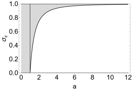
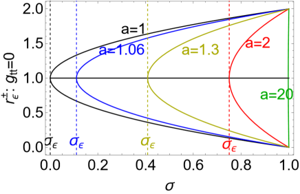
Figure 1: Left panel: Plane $\sigma_{\epsilon}$ in Eq. (3) as function of the NS spin $a>1$. The ergoregion is defined for $\sigma\in[\,\sigma_{\epsilon},1\,]$. There is $\sigma\equiv\sin^{2}\theta\in[\,0,1\,]$, where $\sigma=1$ is the equatorial plane. Radius $r=r_{\epsilon}^{+}=2$ is the outer-ergosurface on the equatorial plane. Right panel: the curves (ergosurfaces) $r_{\epsilon}^{\pm}$ such that $g_{tt}(r_{\epsilon}^{\pm})=0$ are plotted for selected spin, signed on the panel in different colors on the plane $(r,\sigma)$. The limiting values $\sigma_{\epsilon}$ for each spin are also shown as vertical colored dashed lines. There is $g_{tt}>0$ in the region bounded by the curves $r_{\epsilon}^{\pm}$. See analysis in Eq. (3). All quantities are dimensionless.

The role of the limit $\sigma_{\epsilon}$ in the NS geometries is a main difference with the BH cases—see Figs (1). For very fast super-spinning NSs $(a\gg M)$, there is $\sigma_{\epsilon}\to 1$ and the range for the existence of the ergoregion narrows /at $a=M$ there is $\sigma_{\epsilon}=0)$–Figs (1). In the following, where appropriate, to easy the reading of complex expressions, we will use the units with $M=1$ (where $r\rightarrow r/M$ and $a\rightarrow a/M$).

Constants of motion

We consider the following constant of geodesic motions

$$\mathcal{E}=-(g_{t\phi}\dot{\phi}+g_{tt}\dot{t}),\quad\mathcal{L}=g_{\phi\phi}\dot{\phi}+g_{t\phi}\dot{t},\quad g_{ab}u^{a}u^{b}=\kappa,$$ (4)

defined from the Kerr geometry rotational Killing field $\xi_{\phi}=\partial_{\phi}$, and the Killing field $\xi_{t}=\partial_{t}$ representing the stationarity of the background, with $u^{a}\equiv\{\dot{t},\dot{r},\dot{\theta},\dot{\phi}\}$ where $\dot{q}$ indicates the derivative of any quantity $q$ with respect the proper time or a properly defined affine parameter for the light–like orbits (for $\kappa=0$), and $\kappa=(\pm 1,0)$ is a normalization constant ($\kappa=-1$ for test particles).

The constant $\mathcal{L}$ in Eq. (4) may be interpreted as the axial component of the angular momentum of a test particle following timelike geodesics and $\mathcal{E}$ represents the total energy of the test particle related to the radial infinity, as measured by a static observer at infinity. The velocity components $(u^{t},u^{\phi})$ read

$$u^{t}=\frac{g_{\phi\phi}\mathcal{E}+g_{t\phi}\mathcal{L}}{g_{t\phi}^{2}-g_{\phi\phi}g_{tt}},\quad u^{\phi}=-\frac{g_{t\phi}\mathcal{E}+g_{tt}\mathcal{L}}{g_{t\phi}^{2}-g_{\phi\phi}g_{tt}}.$$ (5)

We introduce also the specific angular momentum $\ell$ and the relativistic angular velocity $\Omega\equiv{u^{\phi}}/{u^{t}}$

$$\ell\equiv\frac{\mathcal{L}}{\mathcal{E}}=-\frac{g_{\phi\phi}u^{\phi}+g_{\phi t}u^{t}}{g_{tt}u^{t}+g_{\phi t}u^{\phi}}=-\frac{g_{t\phi}+g_{\phi\phi}\Omega}{g_{tt}+g_{t\phi}\Omega},\quad\Omega(\ell)=-\frac{g_{t\phi}+g_{tt}\ell}{g_{\phi\phi}+g_{t\phi}\ell}.$$ (6)

By considering definition of constants of geodesic motion $\mathcal{L}$ and $\ell$ in Eq. (4) and Eq. (6) we discuss in Sec. (II.1) the notion of co-rotation and counter-rotation in the Kerr NS spacetime. These definitions will constitute a primary template of analysis of the flows we investigate in this work and the inversion surfaces as (newly introduced) geometric properties of the Kerr NSs. Finally, spacetime geodesic structure and tori constraints are the focus of Sec. (II.2). In this section we will explore the circular geodesic co-rotation and counter-rotation motion of the Kerr NSs. These radii constrain the circular test particle geodesics and toroidal extended matter orbiting around the central spinning attractor as, for example, accretion disks. The flows we study are made of matter (test particles) and photons, freely moving towards the central attractor or from the central attractors (we address these different aspects more closely also in Sec. (IV)). The motion is regulated by the geodesic equations and can be parametrized by the constants of motion in Eq. (4). We will use the constant $\ell$, as it is the parameter defining the properties focused in this analysis. It is useful to classify the flows and the characteristics of the accreting structures which could possibly engine the flows, according to the $\ell$ parameter ranges, as studied in Sec. (II.2), where we discuss the flows and accretion tori properties, providing constraints for our set-up.

II.1 On co-rotation and counter-rotation in NSs spacetimes

In this section we introduce some of the constraints and parameters used in this analysis, discussing the specific angular momentum $\ell$ parametrizing the flows, orbiting tori and inversion points. We shall examine both co–rotating and counter—rotating motion with respect to the central attractor, investigating their definitions properties in the Kerr NS spacetimes.

The specific angular momentum $\ell=$constant parametrizes the GRHD barotropic geometrically thick disks– [28]. These toroids are constant pressure surfaces, whose construction in the axes–symmetric spacetimes is based on the application of the von Zeipel theorem. The surfaces of constant angular velocity $\Omega$ and of constant specific angular momentum $\ell$ coincide. The toroids rotation law, $\ell=\ell(\Omega)$, is therefore independent of the details of the equation of state, providing the integrability condition of the Euler equation in the case of barotropic fluids. Consequently, in the geometrically thick disks, the functional form of the angular momentum and entropy distribution, during the evolution of dynamical processes, depends on the initial conditions of the system and not on the details of the dissipative processes [28].

We analyze two families of flows, with fluid specific angular momentum $\ell=\ell^{+}<0$ (counter-rotating) and $\ell=\ell^{-}\lesseqgtr 0$ (co-rotating and counter-rotating) respectively:

$$\ell^{\mp}\equiv\frac{a^{3}\mp r^{3/2}\sqrt{\Delta^{2}}-a(4-3r)r}{a^{2}-(r-2)^{2}r},$$ (7)

[28, 42, 45]. Note that tori are governed by the distribution of specific angular momentum on the equatorial plane, therefore $\ell^{\pm}$ in Eqs (7) are independent of the $\sigma$-coordinate.

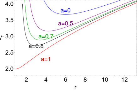
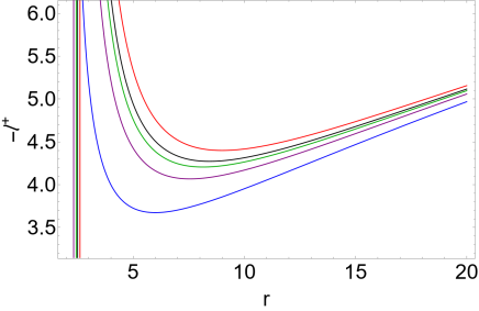
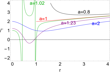
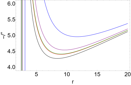
Figure 2: Specific angular momentum $\ell^{+}$ (right column) and $\ell^{-}$ (left column) of Eqs (7) as functions of radius $r$ for different Kerr BH spin $a\in[\,0,1\,]$ (upper line) and BH and NS spin $a>1$ (bottom line) signed on the curves. Right column panels follow the color code explicit in the right panels. (All quantities are dimensionless).

Figs (2) show fluid specific angular momentum $\ell^{\pm}$ as function of $r$ for different spin $a$, for NSs and BHs.

In the NS geometries especially for small values of the spin–mass ratio ($a\in]\,1,a_{2}\,]$ where $a_{2}\equiv 1.29904$) it is necessary to discuss further the notion of co-rotating and counter-rotating motion. Considering quantities of $\{\mathcal{L},\ell\}$, with $a>0$, we introduce the following definitions for fluid and test particle motion:

–

For a circularly orbiting test particle, particle counter–rotation (co-rotation) is defined by $\mathcal{L}a<0$ ($\mathcal{L}a>0$).

–

For fluids, the counter-rotation (co-rotation) is defined by $\ell a<0$ ($\ell a>0$).

We can read these definitions in terms of $\ell$, $\{\mathcal{E},\mathcal{L}\}$ and $\Omega$. (Note the velocity $u^{\phi}$ sign coincides with $\Omega$, assuming $u^{t}>0$). )

For this purpose, it is convenient to introduce radii $\{r_{0}^{\pm},r_{\delta}^{\pm}\}$ defined by the conditions that on the equatorial circular orbits $r_{0}^{\pm}<r_{\epsilon}^{+}=2$, there is $\mathcal{L}=\ell=0$, while on the orbits $r_{\delta}^{\pm}:r_{0}^{-}<r_{\delta}^{-}<r_{\delta}^{+}<r_{0}^{+}$, there is $\mathcal{E}=0$ and $\mathcal{L}<0$ see Figs (3) and [44, 43, 42, 22]. That is radii $r_{0}^{\pm}$ can be found from the condition $\mathcal{L}=\ell=0$ on the geodesic motion and $r_{\delta}^{\pm}$ can be found from the condition $\mathcal{E}=0$ on the geodesic motion. Their explicit form is in Appendix (A). From the analysis of $r_{\delta}^{\pm}$ and $r_{0}^{\pm}$ we introduce the spins,

$$a_{0}:r_{\delta}^{+}=r_{\delta}^{-}\equiv\frac{4}{3}\sqrt{\frac{2}{3}}=1.08866,\quad a_{2}:r_{0}^{+}=r_{0}^{-}\equiv\frac{3\sqrt{3}}{4}=1.29904.$$ (8)

–see Figs (3). Hence spins $a_{0}$ and $a_{2}$ can be found assuming conditions $r_{\delta}^{+}=r_{\delta}^{-}$ and $r_{0}^{+}=r_{0}^{-}$ respectively, and represent a limiting case, where in these NS spacetimes there is only one limiting orbit where $\mathcal{E}=0$ and $\mathcal{L}=0$ respectively (Figs (3)). As detailed below $a_{0}$ and $a_{2}$ are maximum spin where radii $r_{\delta}^{\pm}$ and $r_{0}^{\pm}$ exist. Therefore, we can summarize the situation for counter-rotating flows and co-rotating flows as follows:

Counter-rotating tori $(\ell<0)$

This case includes fluids with $\ell=\ell^{+}<0$ and $\ell=\ell^{-}<0$ in the ergoregion for NSs with $a\in\,[\,1,a_{2}\,]$, more precisely there are:

• Tori with $\ell=\ell^{+}<0$, that is with $(\mathcal{L}<0,\mathcal{E}>0)$ (located far from the ergoregion)
  

• Tori with momentum $\ell=\ell^{-}<0$, that is with $(\mathcal{L}<0,\mathcal{E}>0)$, in $]\,r_{0}^{-},r_{\delta}^{-}\,[\,\cup\,]\,r_{\delta}^{+},r_{0}^{+}\,[$, for spacetimes $a\in\,[\,1,a_{0}\,]$, and in the orbital region $]\,r_{0}^{-},r_{0}^{+}\,[$, for NSs with spin $a\in\,]\,a_{0},a_{2}\,]$–Figs (3).

Co-rotating tori ($\ell>0$)

Co-rotating tori, i.e. with $\ell=\ell^{-}>0$, are defined for $(r>0,a>a_{2})$, $(r\in\,]\,0,r_{0}^{-}\,[\,\cup\,]\,r_{0}^{+},+\infty\,[,a\in\,]\,a_{0},a_{2}\,[\,)$ and $(r\in\,]\,0,r_{0}^{-}\,[\,\cup\,]\,r_{\delta}^{-},r_{\delta}^{+}\,[\,\cup\,r>r_{0}^{+},a\in\,]\,1,a_{0}\,[\,)$–see Figs (3).

$\mathcal{L}$ test particles angular momentum (constant of motion)	Eq.(4)
$\mathcal{E}$ test particles energy (constant of motion)	Eq.(4)
$\ell\equiv\mathcal{L}/\mathcal{E}$ specific angular momentum (constant of motion)	Eq. (6)
$\ell^{+}$ counter-rotating specific angular momentum	Eq. (7)–Sec. (II.1)
$\ell^{-}$ co-rotating or counter-rotating specific angular momentum	Eq. (7)–Sec. (II.1)
$\sigma_{\epsilon}:r_{\epsilon}^{+}=r_{\epsilon}^{-}$	Eq. (3)
$r_{\delta}^{\pm}:\mathcal{E}(r_{\delta}^{\pm})=0,\mathcal{L}(r_{\delta}^{\pm})<0$	Figs (3)– Appendix (A)
$r_{0}^{\pm}:\mathcal{L}(r_{0}^{\pm})=\ell(r_{0}^{\pm})=0$	Figs (3)–Sec. (II.1)–Appendix (A)
$a_{0}:r_{\delta}^{+}=r_{\delta}^{-}\equiv\frac{4}{3}\sqrt{\frac{2}{3}}=1.08866$	Eqs (8)– Figs (3)
$a_{2}:r_{0}^{+}=r_{0}^{-}\equiv\frac{3\sqrt{3}}{4}=1.29904$	Eqs (8)– Figs (3)
${r}_{[mb]}^{\pm}:\;\ell^{\pm}(r_{mb}^{\pm})=\ell^{\pm}({r}_{[mb]}^{\pm})\equiv{\ell_{mb}^{\pm}}$	Eq. (9)–Figs (3)
$r_{[\gamma]}^{\pm}:\ell^{\pm}(r_{\gamma}^{\pm})=\ell^{+}(r_{[\gamma]}^{+})\equiv\ell_{\gamma}^{+}$	Eq. (9)–Figs (3)
$a_{1}\equiv 1.28112:\bar{r}_{ms}^{-}=\tilde{r}_{ms}^{-}$	Sec. (II.2)
$r_{\mbox{\scriptsize{{T}}}}^{\mp}(a,\sigma;\ell):u^{\phi}=0$ inversion radius	Eq. (12)– Figs. (7)– Figs. (8)– Figs. (4)
$\sigma_{\mbox{\scriptsize{{T}}}}(a,r;\ell):u^{\phi}=0$ inversion plane	Eq. (12)
$()_{\mbox{\scriptsize{{T}}}}$ any quantitiy $()$ evaluated on the inversion surface	Sec. (III)
$r_{cr}:r_{\mbox{\scriptsize{{T}}}}^{-}=r_{\mbox{\scriptsize{{T}}}}^{+}$	Eq. (13)– –Figs (5),(6),(7),(8)
$r_{{\mbox{\scriptsize{{T}}}}\max}^{0}:\partial_{a}\sigma_{\mbox{\scriptsize{{T}}}}=0$	Eq. (17)–Figs (11)
$r_{{\mbox{\scriptsize{{T}}}}\max}^{\pm}:\partial_{r_{\mbox{\scriptsize{{T}}}}}\sigma_{\mbox{\scriptsize{{T}}}}=0$	Eq. (17)–Figs (11)
$\ell_{e}^{-}:\partial_{a}r_{\mbox{\scriptsize{{T}}}}^{\pm}=0$	Eqs. (18), Eqs. (19)–Figs (12).

Table 1: Lookup table containing the main notation and quantities used throughout this paper. Links to associated sections, definitions or figures are also listed.

There is therefore $\ell^{-}<0$ with $(\mathcal{L}<0,\mathcal{E}>0)$ in the NS ergoregion, together with co-rotating solutions $\ell^{-}>0$ with $(\mathcal{L}<0,\mathcal{E}<0)$ with negative energy $\mathcal{E}$. However, these solutions correspond to the relativistic angular velocity, i.e. the Keplerian velocity with respect to static observers at infinity, $\Omega>0$. In this sense, they are all co-rotating with respect to the static observers at infinity.

II.2 Extended geodesic structure and tori constraints

Test particle motion and many aspects of the physics of accretion around compact objects is constrained by the spacetime geodesic structure. The flow dynamics we consider in this analysis is regulated by the set of co-rotating and counter-rotating Kerr NSs circular equatorial geodesics radii. This set of radii defines and constrains different extended orbiting surfaces, as accretion tori having different topology and their instability points. It is therefore useful to consider here in details the spacetime co–rotating and counter–rotating geodesic structure.

The Kerr NS background geodesic structure is constituted by the radii $\{r_{\gamma}^{\pm},r_{mb}^{\pm},r_{ms}^{\pm}\}$, marginally circular (photon) orbit, marginally bounded orbit, and marginally stable orbit respectively, regulating the location of the tori and proto-jets cusps. (For convenience we report in Appedix (A) the explicit expression of the radii of the Kerr NS spacetime geodesc structure). The geodesic structure is extended to include radii $\{r_{[\gamma]}^{\pm},r_{[mb]}^{\pm},r_{[ms]}^{\pm}\}$ regulating the location of the toroidal configurations centers :

$${r}_{[mb]}^{\pm}:\;\ell^{\pm}(r_{mb}^{\pm})=\ell^{\pm}({r}_{[mb]}^{\pm})\equiv{\ell_{mb}^{\pm}},\quad r_{[\gamma]}^{\pm}:\ell^{\pm}(r_{\gamma}^{\pm})=\ell^{+}(r_{[\gamma]}^{+})\equiv\ell_{\gamma}^{+},$$ (9)

$$\mbox{where}\quad r_{\gamma}^{\pm}<r_{mb}^{\pm}<r_{ms}^{\pm}<{r}_{[mb]}^{\pm}\quad\mbox{and}\quad{r}_{[mb]}^{+}<r_{[\gamma]}^{+}<r_{\gamma}^{-}\equiv 0,$$ (10)

respectively where there is $r_{\gamma}^{-}\equiv 0$. Increasing the NS spin, radii of geodesic structure and tori depart from the central singularity, for both co-rotating and counter-rotating fluids, constituting a major difference with the BH case. Note there is $r_{[ms]}^{+}=r_{ms}^{+}$ where $r_{[ms]}^{+}:\ell_{ms}^{+}\equiv\ell(r_{ms}^{+})=\ell^{+}(r)$, analogously a similar relation holds for fluids with $\ell^{-}$ at NSs spins $a>a_{2}$.

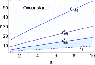
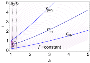
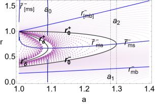
Figure 3: Analysis of co-rotating and counter-rotating tori. Curves $\ell^{-}=$constant (right and center panel) and $\ell^{+}$=constant (left panel) ($\ell^{+}<0$ and $\ell^{-}\lesseqgtr 0$ are the fluid specific angular momentum) in the plane $r-a$. (All quantities are dimensionless). Right panel is a zoom of the center panel. $r_{\gamma}^{\pm}$ are the last circular orbit (there is $r_{\gamma}=0$). There is $r_{0}^{\pm}:\mathcal{L}=\ell=0$. Radii $r_{mb}^{\pm}$ are the marginally bounded orbits. Spins $\{a_{0},a_{2}\}$ are defined in Eqs (8), $a_{1}\equiv 1.28112:\bar{r}_{ms}^{-}=\tilde{r}_{ms}^{-}$ is defined in Sec. (II.2). Radii $r_{ms}^{-}=\{\tilde{r}_{ms}^{-},\bar{r}_{ms}^{-}\}$ and $r_{ms}^{+}$ are the marginally stable orbits for the fluid with specific angular momentum $\ell^{-}$ and $\ell^{+}$ respectively defined in Eqs (7). Radii $r_{[mb]}^{\pm}$ are in Eqs (9). Radii of the geodesic structures are in Appendix (A).

The situation for fluid with momentum $\ell^{-}$ is however more complex. There is $\ell^{-}\lesseqgtr 0$, constrained by the radii $\{r_{mb}^{-},\tilde{r}_{ms}^{-},\bar{r}_{ms}^{-},r_{\gamma}^{-}\}$, with $\{\mathcal{L}\lesseqgtr 0,\mathcal{E}\lesseqgtr 0\}$. Radii $r_{ms}^{-}=\{\bar{r}_{ms}^{-},\tilde{r}_{ms}^{-}\}$, are the marginally stable orbits related to the motion $\ell^{-}\gtrless 0$, where $r_{ms}^{-}=\bar{r}_{ms}^{-}$ for $a>a_{1}$ and $r_{ms}^{-}=\tilde{r}_{ms}^{-}$ for $a\in\,]\,1,a_{1}\,]$ and $\bar{r}_{ms}^{-}=\tilde{r}_{ms}^{-}$ on $a_{1}\equiv 1.28112$–Figs (3). However, for simplicity of notation, when it is not necessary to specify, we will use the abbreviated notation $r_{ms}^{-}$ for $\{\bar{r}_{ms}^{-},\tilde{r}_{ms}^{-}\}$.

Barotropic counter-rotating closed quiescent (not cusped tori, regular topology), cusped or open configurations have centers coincident with maximum of pressure and density point in the disk, the tori cusp is the minimum point of pressure and density.

Tori with specific angular momentum $\ell=\ell^{+}<0$ are constrained as follows [44]

–

For $\ell^{+}\in\,\,\mathbf{L_{1}^{+}}\equiv\,]\,\ell^{+}_{mb},\ell^{+}_{ms}\,[$ there are quiescent and cusped tori. The cusp is $r_{\times}\in\,]\,r_{mb}^{+},r_{ms}^{+}\,]$, and the torus center with maximum pressure is $r_{center}\in\,]\,r_{ms}^{+},r_{[mb]}^{+}\,]$;

–

For $\ell^{+}\in\,\mathbf{L_{2}^{+}}\equiv\,[\,\ell^{+}_{\gamma},\ell^{+}_{\mathrm{mb}}\,[$ there are quiescent tori and proto-jets. Proto-jets are open cusped equipotential surfaces. Unstable point, cusp, is on $r_{j}\in\,]\,r_{\gamma}^{+},r_{mb}^{+}\,]\,$ and center with maximum pressure $r_{center}\in\,]\,r_{[mb]}^{+},r_{[\gamma]}^{+}\,]\,$;

–

For $\ell^{+}\in\,\mathbf{L_{3}^{+}}:\ell^{+}<\ell^{+}_{\gamma}$, there are quiescent tori, with center $r_{center}>r_{[\gamma]}^{+}$.

A very large $\ell$ in magnitude is typical of proto-jets or quiescent toroids orbiting far from the central attractor for counter-rotating tori (with $\ell=\ell^{+}<0$) or some co-rotating tori with $\ell=\ell^{-}>0$) in a class of slow rotating NSs.

A more articulated structure characterizes NSs with spin $a\in\,]\,1,a_{2}\,]$ and fluids with $\ell^{-}$ on the equatorial plane ergoregion. For $a>a_{2}$, where $\mathcal{E}>0$ and $\mathcal{L}>0$ $(\ell^{-}>0)$, the geodetical orbital structure for $\ell^{-}$ is similar to the counter-rotating tori with $\ell=\ell^{+}$, where $r_{\gamma}^{-}=0$. For $a\in\,[\,1,a_{0}\,[$, the $\ell^{-}$ geodesic structure is more articulated. For $a\in\,[\,1,a_{2}\,]$, there can be tori with $\ell^{-}<0$ and ($\mathcal{E}>0,\mathcal{L}<0$) in the ergoregion and tori with $\ell^{-}>0$ and ($\mathcal{E}<0,\mathcal{L}<0$). There can be double tori system with $\ell=\ell^{+}=\ell^{-}<0$ or $\ell=\ell^{-}>0$. For tori with centers and cusps located on $r_{0}^{\pm}$ there is $\ell=\mathcal{L}=0$, and tori in the limiting case of $\ell=0$ are considered in Sec. (IV.3). On $r_{\delta}^{\pm}$ ("center" and "cusp" respectively) there is $\mathcal{E}=0$ ($\ell$ is not well defined).

III Flow inversion points

In this section the inversion points and inversion surfaces definitions are introduced and we start with the analysis of the inversion surfaces extremes and limits focusing, in particular, on the location of the inversion points with the respect to the central singularity.

The flow inversion points are defined by the condition $u^{\phi}=0$ on the flow particle velocities, i.e. as points of vanishing axial velocity of the flow motion as related to distant static observers.

From the definition of constant $\ell$ and $\mathcal{E}$, Eqs (4) and Eq. (6), fixed by the orbiting torus, and the inversion point definition we obtain:

$$\ell=-\left.\frac{g_{t\phi}}{g_{tt}}\right|_{\mbox{\scriptsize{{T}}}}=-\frac{2ar_{{\mbox{\scriptsize{{T}}}}}\sigma_{{\mbox{\scriptsize{{T}}}}}}{\Sigma_{\mbox{\scriptsize{{T}}}}-2r_{\mbox{\scriptsize{{T}}}}},\quad\mbox{where}\quad\mathcal{E}_{\mbox{\scriptsize{{T}}}}\equiv-g_{tt}({\mbox{\scriptsize{{T}}}})\dot{t}_{\mbox{\scriptsize{{T}}}},\quad\mathcal{L}_{\mbox{\scriptsize{{T}}}}\equiv g_{t\phi}({\mbox{\scriptsize{{T}}}})\dot{t}_{\mbox{\scriptsize{{T}}}},$$ (11)

where $\mathcal{E}_{\mbox{\scriptsize{{T}}}}$ and $\mathcal{L}_{\mbox{\scriptsize{{T}}}}$ are the energy and momentum of the flow particles at the inversion point. More in general we adopt the notation $q_{\bullet}\equiv q(r_{\bullet})$ for any quantity $q$ evaluated on a radius $r_{\bullet}$. Therefore, notation $q_{\mbox{\scriptsize{{T}}}}$ or $q({\mbox{\scriptsize{{T}}}})$ is for any quantity $q$ considered at the inversion point, and $q_{0}=q(0)$ for any quantity $q$ evaluated at the initial point of the (free-falling) flow trajectories.

These quantities are independent from the normalization condition, being a consequence of the definition of constant $\{\ell,\mathcal{E},\mathcal{L}\}$ only.

Using Eq. (11), we can discuss the existence of the inversion points radii $r_{\mbox{\scriptsize{{T}}}}^{\pm}$ and planes $\sigma_{\mbox{\scriptsize{{T}}}}$, for co-rotating $\ell>0$ or counter-rotating $\ell<0$ fluids, with constant $\ell$, introducing the quantities

$$r_{\mbox{\scriptsize{{T}}}}^{\mp}=\mp\sqrt{a^{2}\left(\sigma_{\mbox{\scriptsize{{T}}}}+\frac{\sigma_{\mbox{\scriptsize{{T}}}}^{2}}{\ell^{2}}-1\right)-\frac{2a\sigma_{\mbox{\scriptsize{{T}}}}}{\ell}+1}-\frac{a\sigma_{\mbox{\scriptsize{{T}}}}}{\ell}+1,\quad\mbox{and}\quad\sigma_{\mbox{\scriptsize{{T}}}}\equiv\frac{\ell\Delta_{\mbox{\scriptsize{{T}}}}}{a(a\ell-2r_{\mbox{\scriptsize{{T}}}})}.$$ (12)

where $\Delta_{\mbox{\scriptsize{{T}}}}$ is $\Delta$ defined at the inversion point–see Fig. (4).

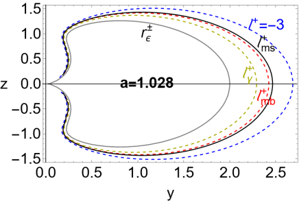
Figure 4: Inversion surfaces $r_{\mbox{\scriptsize{{T}}}}^{\pm}(\ell)$ in the Kerr NS spacetime with spin-mass ratio $a=1.028$, at different counter-rotating specific angular momentum $\ell$ for $\ell\in\{\ell_{\gamma}^{+},\ell_{mb}^{+},\ell_{ms}^{+},-3\}$ as signed on the curves. For $a=1.028$ there is $\ell_{\gamma}^{+}=-7.04659$ (yellow curve), $\ell_{mb}^{+}=-4.84816$ (red curve), $\ell_{ms}^{+}=-4.4173$ (black curve). Hence $\ell_{\gamma}^{+}<\ell_{mb}^{+}<\ell_{ms}^{+}<-3$ and $r_{\epsilon}^{\pm}<r_{\mbox{\scriptsize{{T}}}}(\ell_{\gamma}^{+})<r_{\mbox{\scriptsize{{T}}}}(\ell_{mb}^{+})<r_{\mbox{\scriptsize{{T}}}}(\ell_{ms}^{+})<r_{\mbox{\scriptsize{{T}}}}(-3)$. Gray curves are for radii $r_{\epsilon}^{+}>r_{\epsilon}^{-}$, i.e. the outer and inner ergosurfaces respectively. All the quantities are dimensionless. Notation $ms$ refers the marginally stable circular orbit, $mb$ to marginally bounded orbit and $(\gamma)$ to the marginally circular orbit. There is $r=\sqrt{z^{2}+y^{2}}$ and $\sigma=y^{2}/(z^{2}+y^{2})$, for $\sigma\equiv\sin^{2}\theta$ (where $\sigma=1$ is the equatorial plane).

There is

$$r_{\mbox{\scriptsize{{T}}}}^{-}=r_{\mbox{\scriptsize{{T}}}}^{+}=r_{cr}\equiv a\sqrt{1-\sigma_{\mbox{\scriptsize{{T}}}}}\quad\mbox{on}\quad\ell_{cr}=\frac{a\sigma_{\mbox{\scriptsize{{T}}}}[r_{cr}+1]}{1-r_{cr}^{2}}.$$ (13)

There are no timelike or photon-like inversion points for $\ell>0$, as clear from the study of the conditions $(\mathcal{E},\mathcal{L})$ constant and normalization condition. Radius $r_{cr}$ is shown in Figs (5),(6),(7),(8).

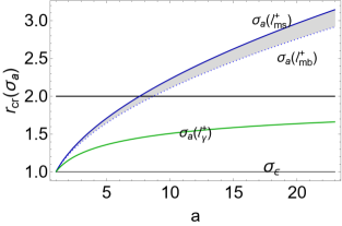
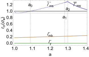
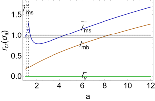
Figure 5: Panels show radius $r_{cr}:r_{{\mbox{\scriptsize{{T}}}}}^{-}=r_{\mbox{\scriptsize{{T}}}}^{+}$ (flow inversion point radius) defined in Eq. (13) on the plane $\sigma_{a}(\ell)$ for different fluid specific angular momenta $(\ell)$, as function of the NS spin $a>1$. Left panel shows the analysis for the counter-rotating fluid specific angular momentum $\ell^{+}<0$. Center and right panels show the analysis for the momentum $\ell^{-}$. Central panel is a close-up view of the right panel. Plane $\sigma_{\epsilon}$ is defined in Eq. (3), the plane $\sigma_{a}$ is defined in Eq. (25). The ergoregion is defined for $\sigma\in[\,\sigma_{\epsilon},1\,]$. There is $\sigma\equiv\sin^{2}\theta\in[\,0,1\,]$, where $\sigma=1$ is the equatorial plane. Notation $(mb)$ is for quantities evaluated on the marginally bounded orbit, $(ms)$ for marginally stable orbit, $(\gamma)$ for marginally circular orbit. Radius $r=r_{\epsilon}^{+}=2$ is the outer-ergosurface on the equatorial plane. Spins $\{a_{0},a_{2}\}$, vertical dotted lines, are defined in Eqs (8) and $a_{1}\equiv 1.28112:\bar{r}_{ms}^{-}=\tilde{r}_{ms}^{-}$ is defined in Sec. (II.2). There is $r_{ms}^{-}\equiv\{\tilde{r}_{ms}^{-},\bar{r}_{ms}^{-}\}$, respectively there is $\{\tilde{\ell}_{ms}^{-},\bar{\ell}_{ms}^{-}\}$–see Sec. (II.2). Here the most general solutions $r_{\mbox{\scriptsize{{T}}}}^{\pm}$ of Eqs (12) are shown. (All quantities are dimensionless).

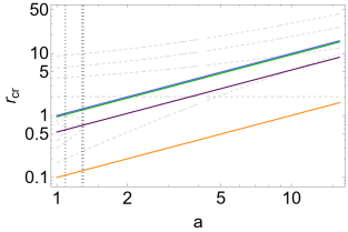
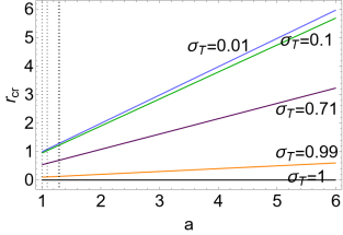
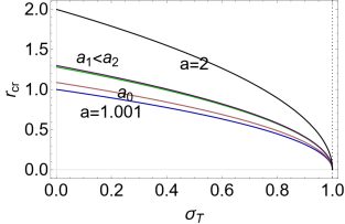
Figure 6: Analysis of counter-rotating flow inversion points $r_{\mbox{\scriptsize{{T}}}}^{\pm}$ with fluid specific angular momentum $\ell^{+}<0$. (Most general solutions $r_{\mbox{\scriptsize{{T}}}}^{\pm}$ are shown, discussion on further constraints on the constants of motion is in Sec. (IV).) Left panel shows in light-gray dashed curves the geodesic structure of the NSs as in Figs (3). Dotted vertical lines are the spins $a_{0}<a_{1}<a_{2}$. Spins $\{a_{0},a_{2}\}$ are defined in Eqs (8) and $a_{1}\equiv 1.28112:\bar{r}_{ms}^{-}=\tilde{r}_{ms}^{-}$ is defined in Sec. (II.2). Radius $r_{cr}=r_{\mbox{\scriptsize{{T}}}}^{\pm}$ of Eq. (13) is shown as function of the NS spin-mass ratio $a$, at different planes $\sigma\equiv\sin^{2}\theta$ signed on the curves (left and center panels), where $\sigma=1$ is the equatorial plane, and as function of the plane $\sigma\in[\,0,1\,]$, for different spins, signed on the curves (right panel). (All quantities are dimensionless).

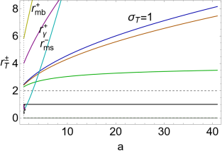
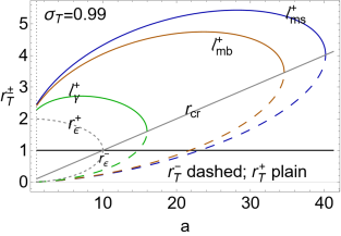
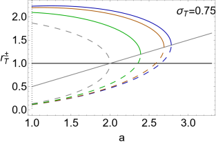
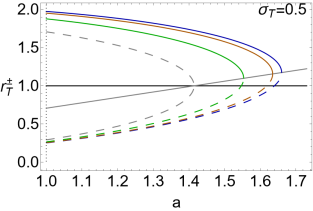
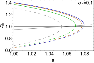
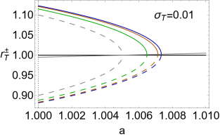
Figure 7: Inversion points $r_{\mbox{\scriptsize{{T}}}}^{\pm}$ of Eqs (12) are shown as functions of the NS spin-mass ratio $a$, for different planes $\sigma\equiv\sin^{2}\theta$ signed on the panels, where $\sigma=1$ is the equatorial plane. (Here the most general solutions $r_{\mbox{\scriptsize{{T}}}}^{\pm}$ are shown, while discussion on the constants of motion is in Sec. (IV).) Dashed gray curves are the outer and the inner ergosurfaces $r_{\epsilon}^{+}\geq r_{\epsilon}^{-}$ respectively. Plain curves are $r_{\mbox{\scriptsize{{T}}}}^{+}$, while $r_{\mbox{\scriptsize{{T}}}}^{-}$ are dashed curves. Curves $r_{\mbox{\scriptsize{{T}}}}^{\pm}(\ell)$ for $\sigma=1$ are generally non linear functions of the spin $a$ when evaluated on the function of the spin $\ell=\ell^{+}(a)\in\,\{\ell_{ms}^{+},\ell_{mb}^{+},\ell_{\gamma}^{+}\}$. The radii are evaluated for the counter-rotating fluid specific angular momentum $\ell=\ell^{+}<0$, on the marginally stable orbit $(ms)$-(darker-blue curve), marginally bounded orbit $(mb)$–(blue-curves) and marginally circular orbit $r_{\gamma}^{+}$ (light-blue curves). Radius $r_{cr}=r_{\mbox{\scriptsize{{T}}}}^{\pm}$ (plain gray line) is defined in Eq. (13). Radius $r_{ms}^{-}$ is the marginally stable orbit for fluid with $\ell=\ell^{-}$. (All quantities are dimensionless).

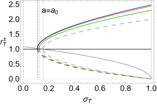
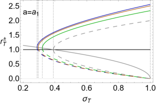
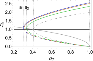
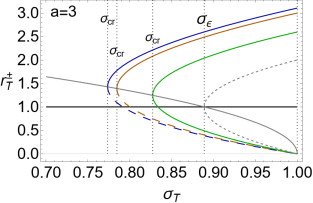
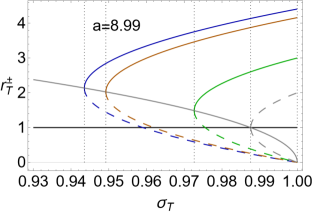
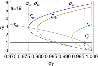
Figure 8: Inversion points $r_{\mbox{\scriptsize{{T}}}}^{\pm}$ of Eqs (12) of the counter-rotating flows with specific angular momentum $\ell^{+}<0$ as functions of the planes $\sigma\equiv\sin^{2}\theta$, for different NS spin-mass ratio $a$ signed on the panels, where $\sigma=1$ is the equatorial plane. (All quantities are dimensionless). Plain curves are $r_{\mbox{\scriptsize{{T}}}}^{+}$, while $r_{\mbox{\scriptsize{{T}}}}^{-}$ are dashed curves. Spins $\{a_{0},a_{2}\}$ are defined in Eqs (8) and $a_{1}\equiv 1.28112:\bar{r}_{ms}^{-}=\tilde{r}_{ms}^{-}$ is defined in Sec. (II.2). Limiting plane $\sigma_{cr}$ is function $\sigma_{a}$ of Eqs (25) evaluated on the selected fluid specific angular momentum. Dashed gray curves are the outer and the inner ergosurfaces $r_{\epsilon}^{+}\geq r_{\epsilon}^{-}$ respectively. Inversion points are evaluated at specific angular momentum on the marginally stable orbit $(ms)$-(darker-blue curve), marginally bounded orbit $(mb)$–(blue-curves) and marginally circular orbit $r_{\gamma}^{+}$ (light-blue curves). See also Figs (7). (The most general solutions $r_{\mbox{\scriptsize{{T}}}}^{\pm}$ are shown not considering the constants of motion analysis of Sec. (IV).)

Quantities $(\sigma_{\mbox{\scriptsize{{T}}}}(r_{\mbox{\scriptsize{{T}}}}),r_{{\mbox{\scriptsize{{T}}}}}(\sigma_{{\mbox{\scriptsize{{T}}}}}))$ depend on the constant of motion $\ell$ only, describing both matter and photons, are independent from the initial particles velocity ($\{\dot{\sigma}_{{\mbox{\scriptsize{{T}}}}},\dot{r}\}$, therefore their dependence on the tori models and accretion process is limited to the dependence on the fluid specific angular momentum $\ell$, and the results considered here are adaptable to a variety of different general relativistic accretion models. Function $r_{\mbox{\scriptsize{{T}}}}=r_{\mbox{\scriptsize{{T}}}}^{\pm}(\sigma)$ (equivalently $\sigma_{\mbox{\scriptsize{{T}}}}(r_{\mbox{\scriptsize{{T}}}})$) defines an almost continuous locus of inversion points, surrounding the central singularity, inversion surface, where the condition $u^{\phi}=0$ is satisfied. For flows from the orbiting tori there is a maximum and a minimum boundary $r_{\mbox{\scriptsize{{T}}}}(a;\ell,\sigma_{\mbox{\scriptsize{{T}}}})$, associated to a maximum and minimum value of $\ell$. This region, as well as its boundaries, will be called the inversion corona. The extremes of $\ell$ parameters are determined by the tori parametrized with $\ell$. Therefore, the accretion driven inversion corona has boundaries defined by $r_{\mbox{\scriptsize{{T}}}}^{\pm}$ (or $\sigma_{\mbox{\scriptsize{{T}}}}$), evaluated on $\ell_{ms}^{\pm}$ and $\ell_{mb}^{\pm}$, while the proto-jets driven coronas has (in general) boundaries defined by $r_{\mbox{\scriptsize{{T}}}}^{\pm}$ (or $\sigma_{\mbox{\scriptsize{{T}}}}$), evaluated on $\ell_{mb}^{\pm}$ and $\ell_{\gamma}^{\pm}$–Fig. (4). In Sec. (III.0.1), the inversion radii and inversion plane extremes and limits are discussed. We focus on the necessary conditions for the existence of the inversion points of the counter-rotating and co-rotating flows in Sec. (IV), considering first the condition $\ell=$constant and then $\{\ell,\mathcal{E},\mathcal{L}\}$ constant.

III.0.1 Extremes and limits of the flows inversion points

We consider functions $r_{\mbox{\scriptsize{{T}}}}^{\pm}$ in all generality, considering $\ell$ constant, but not taking into account the condition of normalization or the conditions on the signs of $(\mathcal{E},\mathcal{L})$. There is

$$\lim_{\sigma_{\mbox{\scriptsize{{T}}}}\rightarrow 0}r_{{\mbox{\scriptsize{{T}}}}}^{\pm}=r_{\pm},\quad\lim_{\ell\rightarrow(\pm\infty)}r_{{\mbox{\scriptsize{{T}}}}}^{\pm}=r^{\pm}_{\epsilon}\quad\mbox{respectively and}\quad\lim_{a\rightarrow+\infty}\sigma_{\mbox{\scriptsize{{T}}}}=1,\quad\lim_{\ell\rightarrow\pm\infty}\sigma_{\mbox{\scriptsize{{T}}}}=\sigma_{erg}.$$ (14)

The last limit is well defined (i.e. $\sigma_{\mbox{\scriptsize{{T}}}}\in[\,0,1\,]$), only for $r_{\mbox{\scriptsize{{T}}}}\leq 2$–Figs (9).

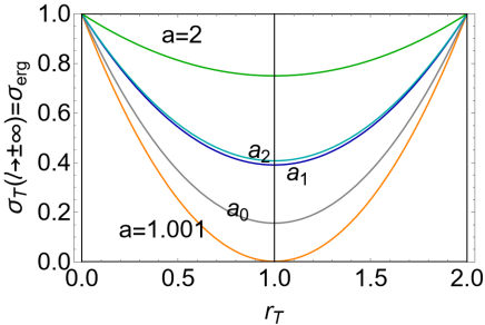
Figure 9: Analysis of the inversion point plane $\sigma_{\mbox{\scriptsize{{T}}}}$ considered in Sec. (IV.1.2). Here the most general solution $\sigma_{\mbox{\scriptsize{{T}}}}$ is shown, not considering the further constraints of Sec. (IV)). Limit for large specific angular momentum magnitude, defined in Eq. (14), coincident with the ergosurface $\sigma_{erg}$ defined in Eqs. (2), for different NSs spin-mass ratios signed on the curves. Spins $\{a_{0},a_{2}\}$ are defined in Eqs (8) and $a_{1}\equiv 1.28112:\bar{r}_{ms}^{-}=\tilde{r}_{ms}^{-}$ is defined in Sec. (II.2). (All quantities are dimensionless).

The limit of the inversion radii on the poles is well defined in the BH case only. The limit for large specific angular momentum in magnitude is independent from the co-rotation or counter-rotation flow direction. As noted also for the BH case, in the limit for large magnitude of the specific angular momentum, the inversion point approaches the ergosurface, from above or from below, if the flow is counter-rotating or co-rotating (this issue is detailed in Secs (IV)). A very large $\ell$ in magnitude is typical of proto-jets emission or quiescent toroids orbiting far from the central attractor for counter-rotating tori (with $\ell=\ell^{+}<0$) or some co-rotating tori with $\ell=\ell^{-}>0$) in a class of slow rotating NSs. The limit of $r_{\mbox{\scriptsize{{T}}}}=r_{\mbox{\scriptsize{{T}}}}^{\pm}$ for $a\rightarrow+\infty$ (a very faster spinning NS) is not well defined. Increasing the spin $a>0$, the inversion point approaches the equatorial plane $(\sigma_{\mbox{\scriptsize{{T}}}}\leq 1)$–Figs (9,10,7,8). It is interesting to note that, contrary to the BH case, in the NS there can be two inversion points radii $r_{\mbox{\scriptsize{{T}}}}^{\pm}$.

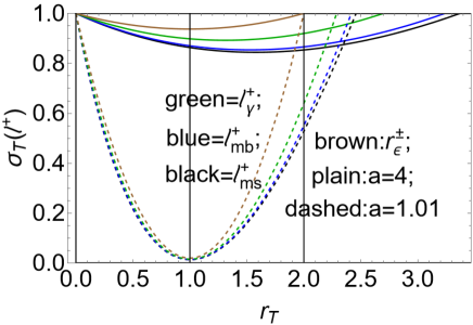
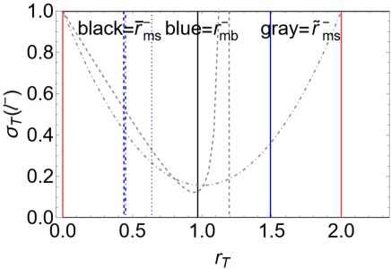
Figure 10: Inversion point plane $\sigma_{\mbox{\scriptsize{{T}}}}$ considered in Sec. (IV.1.2) evaluated on the specific angular momentum $\ell^{+}$ (left panel) and $\ell^{-}$ (right panel) as function of the inversion radius $r_{\mbox{\scriptsize{{T}}}}$. Here the most general solution $\sigma_{\mbox{\scriptsize{{T}}}}$ is shown, not considering the further constraints of Sec. (IV)). (All quantities are dimensionless). There is $\sigma\equiv\sin^{2}\theta\in[\,0,1\,]$, and $\sigma=1$ is the equatorial plane. Left panel: counter-rotating inversion planes for counter-rotating flows $\ell=\ell^{+}<0$ evaluated at specific angular momentum on the marginally stable orbit $(ms)$, marginally bounded orbit $(mb)$ and marginally circular orbit $r_{\gamma}^{+}$, for different spin-mass ratios, as functions of the radius inversion point. Radius $r_{ms}^{-}=\{\bar{r}_{ms}^{-},\tilde{r}_{ms}^{-}\}$ is the marginally stable orbit, $r_{mb}^{-}$ is the marginally bounded orbit, for $\ell=\ell^{-}$. Right panel: Analysis of the inversion point radius $r_{\mbox{\scriptsize{{T}}}}$ and plane $\sigma_{\mbox{\scriptsize{{T}}}}$ from accretion flows with specific angular momentum $\ell=\ell^{-}$. Dashed curve is for $a=1.01$; dotted - dashed curve is for $a=a_{0}$, dotted curve is for $a=a_{2}$, plain curve for $a=2$. Spins $\{a_{0},a_{2}\}$ are defined in Eqs (8).

We proceed below as follows: we first consider the inversion surfaces morphology analysing the critical radius $r_{cr}$, defined as $r_{cr}=r_{\mbox{\scriptsize{{T}}}}^{+}=r_{\mbox{\scriptsize{{T}}}}^{-}$, which provides indication on the inversion surface radial structure, as the maximum radial distance from the central spinning attractor, according to the NS spin and flow parameters. Secondly, we concentrate our attention on the inversion points in the regions close to the singularity poles. The inversion surfaces is in fact in some cases not well defined in the region. On the other hand, in other cases the particular structure of the surfaces close the poles singles out this special region of the spacetime by the effects associated to the presence of the inversion points–see Fig. (4. In this framework, it could be expected that this region may be of interest for jet emission (having funnels along the rotational axis) or other flows coming towards the singularity poles on the vertical direction. However, most of the accretion flows of the common scenarios currently under scrutiny concerns the singularity equatorial plane. For example, accretion from a disk inner edge is usually considered from the inner part of the disk laid on the attractor (and disk) equatorial plane. Hence, we will give particular attention to the inversion surfaces on the equatorial plane. This part of our analysis is then finalized by the discussion of the surfaces extreme points. By representing the inversion surfaces in the plane $(r,\sigma)$, we start examining the extremes of the inversion plane $\sigma_{\mbox{\scriptsize{{T}}}}$ according to the flow parameter $\ell$, or the NS spin $a$ and finally to the inversion radius $r_{\mbox{\scriptsize{{T}}}}$. In this way we closely relate the inversion surfaces to the flows properties, considering variation of the inversion plane with the respect to the flow specific angular momentum at different $a$ and radius $r_{\mbox{\scriptsize{{T}}}}$. We will show also that there is in fact an extreme of the poloidal angle at the inversion point as function of the central singularity spin, showing that the inversion surfaces can show strongly different features for different attractors. Fixing $a$ and flow momentum $\ell$, we proceed considering a general inversion surface expressed as the function $\sigma_{\mbox{\scriptsize{{T}}}}(r_{\mbox{\scriptsize{{T}}}})$, tracing its profiles examining the zeros of the function $\partial_{r_{\mbox{\scriptsize{{T}}}}}\sigma_{\mbox{\scriptsize{{T}}}}$. Results of this analysis are also confirmed by the examination of the maxima and minima of the inversion radius function $r_{\mbox{\scriptsize{{T}}}}$, with respect to the spin $a$, the flow $\ell$, providing the maximum and minimum radial distance of the inversion point from the central singularity, with the respect to the NS spin or the parameter $\ell$. This study ultimately fixes the vertical and radial extension of the inversion surfaces which are spacetime geometrical properties defined as toroidal surfaces embedding the central singularity (ergoregions) presenting a complex structure in the region close to the attractor poles and with a non–trivial variation with the spin of the singularity.

On the boundary radius $r_{\mbox{\scriptsize{{T}}}}^{\pm}=r_{cr}$

The inversion radius $r_{\mbox{\scriptsize{{T}}}}(\sigma_{\mbox{\scriptsize{{T}}}})$ depends on the geometry and torus parameter $(a,\ell)$, while $r_{cr}$, of Eqs (13) is a background property, independent explicitly from $\ell$. It represents a boundary value for $r_{\mbox{\scriptsize{{T}}}}^{\pm}$–see Figs (7,8,6). Radius $r_{\mbox{\scriptsize{{T}}}}(\sigma_{\mbox{\scriptsize{{T}}}})$ provides a good indication of the maximum extension of the inversion point for $\sigma$ and for $a$, as shown for the counter-rotating case in Figs (7), Figs (8). From Figs (6), we can note that the inversion radius $r_{\mbox{\scriptsize{{T}}}}^{\pm}=r_{cr}$ always increases with the NS spin and decreases with the plane $\sigma$, being larger at the poles–Fig. (4). Function $r_{\mbox{\scriptsize{{T}}}}^{\pm}=r_{cr}$ has no extremes for plane $\sigma$. There is however $\partial_{a}r_{cr}=0$ on the equatorial plane.

Below we study the maximum geometric extension of the inversion spheres on the equatorial plane and on the vertical direction parallel to the central attractor rotational axis, which is a relevant aspect particularly for proto-jets flows.

Inversion points close to the poles and on the equatorial plane

We concentrate on the inversion points close to the NS poles $\sigma=0$ and on the NS equatorial plane $\sigma=1$. (The inversion surfaces on the equatorial plane are shown in Fig. (4)). There is

$$\sigma_{\mbox{\scriptsize{{T}}}}=0:\ \mbox{for}\quad(\ell=0,r_{\mbox{\scriptsize{{T}}}}>0)\quad\mbox{and}\quad\sigma_{\mbox{\scriptsize{{T}}}}=1:\ \mbox{for}\quad\ell<0\,\cup\,\ell\geq\ell_{\gamma}^{-},\quad r_{\mbox{\scriptsize{{T}}}}=r_{b},\quad\mbox{where}\quad r_{b}\equiv\frac{2(\ell-a)}{\ell}.$$ (15)

In particular there is $\sigma_{\mbox{\scriptsize{{T}}}}=1$ in $r_{\mbox{\scriptsize{{T}}}}>2$ only for $a>1,\ell<0,r_{\mbox{\scriptsize{{T}}}}=r_{b}$. In other words, on the equatorial plane ($\sigma_{\mbox{\scriptsize{{T}}}}=1$) at inversion point, there is

$$\ell_{\beta}\equiv\frac{2a}{2-r},\quad\mbox{or}\quad r_{\mbox{\scriptsize{{T}}}}=r_{b}=\frac{2(\ell-a)}{\ell},$$ (16)

for $\ell<0$ (counter-rotating flows) or for $\ell>\ell_{\gamma}^{-}>0$, whereas there are no solutions for $\ell_{\gamma}^{-}>\ell>0$.

Extremes of the inversion plane $\sigma_{\mbox{\scriptsize{{T}}}}$

Below we analyze the extremes of the inversion plane $\sigma_{\mbox{\scriptsize{{T}}}}$ with respect to the inversion point radius $r_{\mbox{\scriptsize{{T}}}}$, the fluid specific angular momentum $\ell$ and the dimensionless NS spin $a$.

There is

$$\partial_{\ell}\sigma_{\mbox{\scriptsize{{T}}}}=0:\quad\mbox{for}\quad(\ell\neq 0,r_{\mbox{\scriptsize{{T}}}}=0)$$

$$\partial_{a}\sigma_{\mbox{\scriptsize{{T}}}}=0:\quad\mbox{for}\quad(\ell<0,r_{\mbox{\scriptsize{{T}}}}=\{0,r_{{\mbox{\scriptsize{{T}}}}\max}^{0}\}),(\ell=0,r_{\mbox{\scriptsize{{T}}}}>0),(\ell>0,r_{\mbox{\scriptsize{{T}}}}=0),$$

$$\quad\quad\quad\mbox{where}\quad r_{{\mbox{\scriptsize{{T}}}}\max}^{0}\equiv\frac{1}{2}\left[a\ell+2\sqrt{a^{2}\left(\ell^{2}+4\right)+4(1-a\ell)}\right].$$

$$\partial_{r_{\mbox{\scriptsize{{T}}}}}\sigma_{\mbox{\scriptsize{{T}}}}=0:\quad\mbox{for}\quad(\ell<0,r_{\mbox{\scriptsize{{T}}}}=r_{{\mbox{\scriptsize{{T}}}}\max}^{+}),(\ell=0,r_{\mbox{\scriptsize{{T}}}}>0),(\ell=\ell_{\gamma}^{-},r_{\mbox{\scriptsize{{T}}}}=0),(\ell>\ell_{\gamma}^{-},r_{\mbox{\scriptsize{{T}}}}=r_{{\mbox{\scriptsize{{T}}}}\max}^{-}),$$

$$\quad\mbox{with }\quad r_{{\mbox{\scriptsize{{T}}}}\max}^{\mp}\equiv\frac{1}{2}\left[a\ell\mp\sqrt{a\left[a\left(\ell^{2}+4\right)-4\ell\right]}\right],\quad\mbox{where}\quad\sigma_{{\mbox{\scriptsize{{T}}}}\max}^{\pm}\equiv\sigma_{{\mbox{\scriptsize{{T}}}}}(r_{{\mbox{\scriptsize{{T}}}}\max}^{\pm})$$ (17)

–Figs (11).

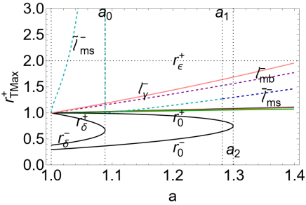
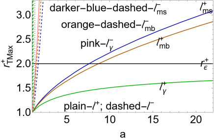
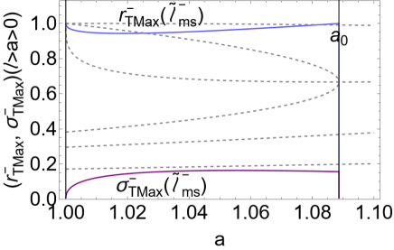
Figure 11: Analysis of the extremes of the flow inversion point plane $r_{{\mbox{\scriptsize{{T}}}}\max}^{\pm}:\partial_{r_{\mbox{\scriptsize{{T}}}}}\sigma_{\mbox{\scriptsize{{T}}}}=0$ of Eqs (18) and maximum inversion plane $\sigma_{{\mbox{\scriptsize{{T}}}}\max}^{+}$ of Eqs (17). Spins $\{a_{0},a_{2}\}$ are defined in Eqs (8) and $a_{1}\equiv 1.28112:\bar{r}_{ms}^{-}=\tilde{r}_{ms}^{-}$ is defined in Sec. (II.2). See also analysis of Secs (IV.1.2). (All quantities are dimensionless). Upper line panels: radius $r_{\max}^{\pm}$ evaluated on the specific angular momenta $\ell^{+}<0$ and $\ell^{-}$ on the marginally bounded orbit $(mb)$, marginally stable orbits $(ms)$– Figs (3). Radius $r_{\epsilon}^{+}=2$ is the outer ergosurface on the equatorial plane. Upper left panel is a close–up view of the right panel. Bottom left panel: the maximum plane $\sigma_{{\mbox{\scriptsize{{T}}}}\max}^{+}\equiv\sigma_{{\mbox{\scriptsize{{T}}}}}(r_{{\mbox{\scriptsize{{T}}}}\max}^{+})$ as function of the NS spin–mass ratio, for different fluid specific angular momenta following the colouring notation of the upper right panel. Inside plot is a close-up view. Bottom right panel: radius $r_{{\mbox{\scriptsize{{T}}}}\max}^{-}$ and plane $\sigma_{{\mbox{\scriptsize{{T}}}}\max}^{-}\equiv\sigma_{{\mbox{\scriptsize{{T}}}}}(r_{{\mbox{\scriptsize{{T}}}}\max}^{-})$ on the fluid specific angular momentum $\tilde{\ell}_{ms}^{-}\equiv\ell^{-}(\tilde{r}_{ms}^{-})>a>0$. Dashed-gray curves are the Kerr NS geodesic structure. (In this analysis the most general solutions $r_{\mbox{\scriptsize{{T}}}}^{\pm}$ are shown not considering the constants of motion analysis of Sec. (IV).)).

Therefore the inversion surface morphology (plane $\sigma_{\mbox{\scriptsize{{T}}}}$), for photons and particles, differentiates the central attractors by their spin, and the extreme points of the spheres depend on the spin and fluid parameter $\ell$, distinguishing proto-jets from accretion tori.

Extremes of the inversion point radius $r^{\pm}_{\mbox{\scriptsize{{T}}}}$

Radius $r_{cr}$ always decreases with $\sigma\in\,]\,0,1\,[$–see Figs (7,8,6). Whereas there is $\partial_{a}r_{cr}=0$, for the limiting case $\sigma=1$ (the equatorial plane), increasing always with the spin for $\sigma\in\,]\,0,1\,[$. There is $r_{cr}(\sigma\rightarrow 1)=0$.

The extremes of the inversion radii $r_{\mbox{\scriptsize{{T}}}}^{\pm}$ for the dimensionless NS spin $a$ are as follows

$$\partial_{a}r_{\mbox{\scriptsize{{T}}}}^{-}=0:\quad\sigma_{\mbox{\scriptsize{{T}}}}=1,(\ell<0,\ell>\ell_{\gamma}^{-}),\quad\mbox{and}\quad\partial_{a}r_{\mbox{\scriptsize{{T}}}}^{+}=0:(\sigma_{\mbox{\scriptsize{{T}}}}\in\,]\,0,1\,[\,,\ell=\ell_{e}^{-}<0),(\sigma_{\mbox{\scriptsize{{T}}}}=1,\ell\in\,]\,0,\ell_{\gamma}^{-}\,[\,),$$ (18)

$$\mbox{where}\quad\ell_{e}^{-}\equiv\frac{a\sigma_{\mbox{\scriptsize{{T}}}}\left[1+\sqrt{1+r_{cr}^{2}}\right]}{-r_{cr}^{2}}$$ (19)

see–Figs (12) and also Figs (4).

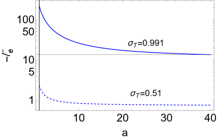
Figure 12: Analysis of the extremes of the flow inversion point radius $r_{\mbox{\scriptsize{{T}}}}^{\pm}$ of Eqs (18). (All quantities are dimensionless). Right panel: fluid specific angular momentum $\ell_{e}^{-}$ defined in Eqs (19), as functions of the spin-mass ratio $a$, for different planes $\sigma\equiv\sin^{2}\theta$ (where $\sigma=1$ is the equatorial plane). Left panel: inversion radii $r_{\mbox{\scriptsize{{T}}}}^{\pm}$ on $\ell_{e}^{-}$ as functions of $a$, for different $\sigma$. Radii $r_{\epsilon}^{+}>r_{\epsilon}^{-}$ are the outer and inner ergosurfaces respectively.

(There are no solutions $\partial_{\sigma_{\mbox{\scriptsize{{T}}}}}r_{\mbox{\scriptsize{{T}}}}^{\pm}=0$, and $\partial_{a}r_{\mbox{\scriptsize{{T}}}}^{+}=0$ for $\ell=0$–Figs (8))

Considering the inversion point radius as function of the fluid specific angular momentum $\ell$, there is

$$\partial_{\ell}r_{\mbox{\scriptsize{{T}}}}^{-}=0:\quad\sigma_{\mbox{\scriptsize{{T}}}}=1\quad(\ell<0,\ell>\ell_{\gamma}^{-}>1);\quad\partial_{\ell}r_{\mbox{\scriptsize{{T}}}}^{+}=0:\quad\sigma_{\mbox{\scriptsize{{T}}}}=1\quad(\ell\in\,]\,0,1\,]\,,\ell_{\gamma}^{-}>\ell>1),$$ (20)

(see also Eqs (15,16)). There are extremes of the inversion point radius, as function of $\ell$ on the equatorial plane.

For the co-rotating flows inversion points ($\ell>0$), as in Eqs (20), (18), (17), (15), condition $\ell>\ell_{\gamma}^{-}>1$, has to be evaluated. (There is $\ell_{\gamma}^{-}=a$, for $\ell^{-}$ evaluated at the last circular co-rotating orbit $r_{\gamma}^{-}=0$ and on $r_{[\gamma]}^{-}=a^{2}$, bottom boundary for the $\mathbf{L_{3}^{-}}$ range.). There is:

$$\ell^{-}=\ell_{\gamma}^{-}:\quad\mbox{for}\quad\left(r=r_{[\gamma]}^{-},a\neq a_{3}\right),(r=0,a\geq 1),\quad\mbox{where}\quad a_{3}\equiv\sqrt{3},$$ (21)

$$\ell^{-}>\ell_{\gamma}^{-}:\quad\mbox{for}\quad a\in\,[\,1,a_{0}\,[\,:\left(r\in\,]\,r_{\delta}^{-},r_{\delta}^{+}\,[\,,r>r_{[\gamma]}^{-},r\neq r_{\delta}^{(1)}\right),$$

$$\;\qquad\qquad\quad\mbox{for}\quad a\in\,[\,a_{0},a_{3}\,[\,:\left(r>r_{[\gamma]}^{-},r\neq r_{\delta}^{(1)}\right),\;$$

$$\;\qquad\qquad\quad\mbox{for}\quad a\geq a_{3}:r>r_{[\gamma]}^{-},$$

where

$$r_{\delta}^{(1)}\equiv\frac{\delta^{+}+\delta^{-}+8}{6},\quad\mbox{and}\quad\delta^{\pm}\equiv 2^{2/3}\sqrt[3]{27a^{2}\pm 3\sqrt{81a^{4}-96a^{2}}-16},$$ (22)

there is $\ell_{\gamma}^{-}=a$ and $r_{[\gamma]}^{-}=a^{2}$–Figs (13).

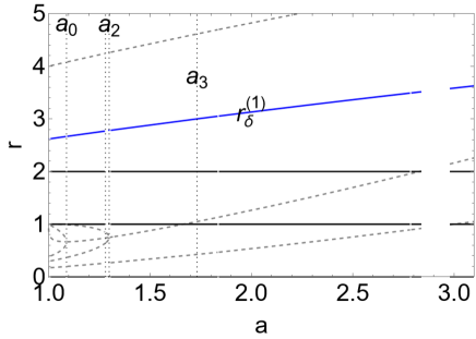
Figure 13: Radius $r_{\delta}^{(1)}$, defined in Eq (22), as function of the NS spin-mass ratio. It refers to the conditions $\ell^{-}\geq a$ of Eqs (21). Gray dashed curves are the geodesic structure of the NSs as in Figs (3). There is $a_{3}=\sqrt{3}$. Spins $\{a_{0},a_{2}\}$ are defined in Eqs (8) and $a_{1}\equiv 1.28112$. (All quantities are dimensionless).

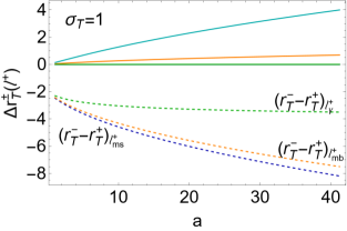
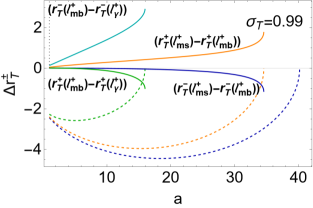
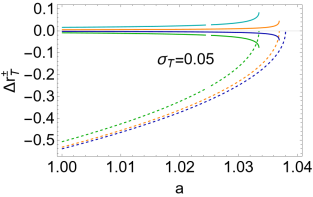
Figure 14: Analysis of the counter-rotating flow inversion radius $r_{\mbox{\scriptsize{{T}}}}^{\pm}$ of Eqs (12) with specific angular momentum $\ell^{+}<0$, as functions of the NS spin-mass ratio $a$, for different planes $\sigma\equiv\sin^{2}\theta$ signed on the panels, where $\sigma=1$ is the equatorial plane. (Here most general solutions $r_{\mbox{\scriptsize{{T}}}}^{\pm}$ shown not considering constraints of Sec. (IV).) Difference $\Delta r_{\mbox{\scriptsize{{T}}}}^{\pm}$ defined on the curves according to the notations of the left and center panels. Inversion points are evaluated at specific angular momentum on the marginally bounded orbit $(mb)$, marginally stable orbit $(ms)$ and marginally circular orbit $r_{\gamma}^{+}$. Dashed curves are differences $(r_{\mbox{\scriptsize{{T}}}}^{-}-r_{\mbox{\scriptsize{{T}}}}^{+})_{\ell}$ at fixed $\ell$. Plain curves are differences $(r_{\mbox{\scriptsize{{T}}}}^{\pm}(\ell_{1})-r_{\mbox{\scriptsize{{T}}}}^{\pm}(\ell_{2}))$ for two fixed values of $\ell$. (All quantities are dimensionless).

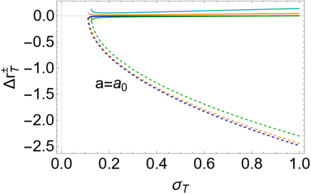
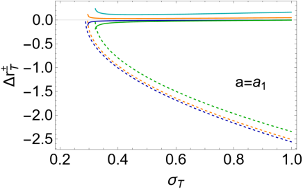
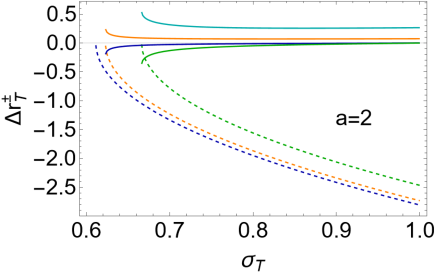
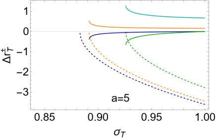
Figure 15: Analysis of the counter-rotating flow inversion radius $r_{\mbox{\scriptsize{{T}}}}^{\pm}$ of Eqs (12) with specific angular momentum $\ell^{+}<0$, as function of planes $\sigma_{\mbox{\scriptsize{{T}}}}=\sigma\equiv\sin^{2}\theta\in[\,0,\,1]$, where $\sigma=1$ is the equatorial plane, for different NS spin-mass ratios signed on the panel. (Here most general solutions $r_{\mbox{\scriptsize{{T}}}}^{\pm}$ shown not considering constraints of Sec. (IV).) Spins $\{a_{0},a_{1}\}$ are defined in Eqs (8). Difference $\Delta r_{\mbox{\scriptsize{{T}}}}^{\pm}$ defined on the curves according to the notations of the left and center panels of Figs (14) . Inversion points are evaluated at specific angular momentum on the marginally bounded orbit $(mb)$, marginally stable orbit $(ms)$ and marginally circular orbit $r_{\gamma}^{+}$. Dashed curves are differences $(r_{\mbox{\scriptsize{{T}}}}^{-}-r_{\mbox{\scriptsize{{T}}}}^{+})_{\ell}$ at fixed $\ell$. Plain curves are differences $(r_{\mbox{\scriptsize{{T}}}}^{\pm}(\ell_{1})-r_{\mbox{\scriptsize{{T}}}}^{\pm}(\ell_{2}))$ for two fixed values of $\ell$. (All quantities are dimensionless).

There are no inversion points for $\ell=\ell^{-}>0$ for $a>a_{2}$. The inversion corona therefore is a closed region, generally of small extension and thickness. The vertical coordinate $z_{\mbox{\scriptsize{{T}}}}$, elongation on the central rotational axis of the inversion point, for the counter-rotating flows, is the order of $\lesssim 1.4$ (central attractor mass, where $r=\sqrt{z^{2}+y^{2}}$ and $\sigma\equiv\sin^{2}\theta=y^{2}/(z^{2}+y^{2})$.).

IV Inversion points of the counter-rotating and co-rotating flows

Inversion point definition, as the set of points where $u^{\phi}=0$ identifies a surface, inversion surface, surrounding the central singularity, depending only on $\ell$ parameter of the freely infalling (or outfalling) matter. The inversion surface is a general property of the orbits in the Kerr NS spacetime. In this article we study in general function $\ell(u^{\phi}=0)$, constraining then $\ell_{\mbox{\scriptsize{{T}}}}$ when framed in the particles flow and tori flows inversion points. We assume: 1. constance of $(\mathcal{E}_{\mbox{\scriptsize{{T}}}},\mathcal{L}_{\mbox{\scriptsize{{T}}}})$ (implied by $\ell=$constant) evaluated at the inversion point with $\dot{t}$>0. 2. We then consider the normalization condition at the inversion point, distinguishing particles and photons in the flow. 3. The matter flow is then related to the orbiting structures, constraining the range of values for $\ell$, to define the inversion corona for proto-jets or accretion driven flows, as background geometry properties, depending only on the spacetime spin. (Inversion surface describes also particles with $\dot{r}_{\mbox{\scriptsize{{T}}}}>0$ (outgoing particles) or particles with an axial velocity $\dot{\theta}\neq 0$ along the BH rotational axis.).

Sign of $\{\ell,\mathcal{L}\}$ at the inversion point for the counter-rotation case is addressed in Sec. (IV.1.3). In this section we explore in details the inversion points of the accreting flows. Specifically, counter-rotating flows $(\ell<0)$ inversion points are detailed in Sec. (IV.1). In Sec. (IV.1.1) we analyze the inversion radius $r_{\mbox{\scriptsize{{T}}}}^{\pm}$, while in Sec. (IV.1.2) we focus on the inversion plane $\sigma_{\mbox{\scriptsize{{T}}}}$. The co-rotating ($\ell>0$) flows inversion points are detailed in Sec. (IV.2).

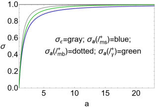
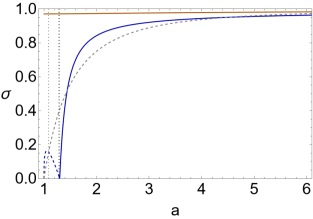
Figure 16: Plane $\sigma_{a}$, defined in Eq. (25), as function of the NS spin-mass ratio $a>1$ evaluated on the counter-rotating fluid specific angular momentum $\ell^{+}<0$ (left panel). Center and right panels show the plane $\sigma_{a}$ for different specific angular momenta $\ell^{-}$, center panel is a close–up view of the right panel. Color notation follows the closed-up view panel. Notation $(mb)$ is for quantities evaluated on the marginally bounded orbit, $(ms)$ for marginally stable orbit, $(\gamma)$ for marginally circular orbit. Plane $\sigma_{\epsilon}$ is defined in Eq. (3). The ergoregion is defined for $\sigma\in[\,\sigma_{\epsilon},\,1]$. There is $\sigma\equiv\sin^{2}\theta\in[\,0,1\,]$, where $\sigma=1$ is the equatorial plane. Dotted vertical lines are spins $a_{0}<a_{1}<a_{2}$, defined in Eqs (8). The marginally stable orbit is $r_{ms}^{-}\equiv\{\tilde{r}_{ms}^{-},\bar{r}_{ms}^{-}\}$, respectively there is $\{\tilde{\ell}_{ms}^{-},\bar{\ell}_{ms}^{-}\}$–see Sec. (II.2). (All quantities are dimensionless).

IV.1 Inversion points of counter-rotating flows

In this section we study the inversion points of counter-rotating flows $(\ell<0)$, considering in Sec. (IV.1.1) the inversion radius $r_{\mbox{\scriptsize{{T}}}}^{\pm}(\sigma)$, while in Sec. (IV.1.2) we explore the inversion plane $\sigma_{\mbox{\scriptsize{{T}}}}(r)$. In Sec. (IV.1.1) and Sec. (IV.1.2) we develop our analysis considering definitions in Eq. (11), derived by the definition of $\ell=$constant and condition $u^{\phi}=0$. Whereas in Sec. (IV.1.3), we discuss the conditions for $u^{\phi}=0$ and $\ell<0$, within $(\mathcal{E},\mathcal{L})$ constant, considering definitions in Eq. (11).

According to the analysis in Sec. (II.1) and Sec. (II.2) we consider (I) tori with $\ell=\ell^{+}<0$, that is with $(\mathcal{L}<0,\mathcal{E}>0)$, located (centered) at $r>r_{\gamma}^{+}$– Figs (7,8,14,15). (II) Tori with momentum $\ell=\ell^{-}<0$, that is with $(\mathcal{L}<0,\mathcal{E}>0)$, in $]\,r_{0}^{-},r_{\delta}^{-}\,[\,\cup\,]\,r_{\delta}^{+},r_{0}^{+}\,[$, for spacetimes $a\in[\,1,\,a_{0}]$, and in the orbital region $]\,r_{0}^{-},r_{0}^{+}\,[$, for NSs with spin $a\in\,]\,a_{0},a_{2}\,]$. The case $\ell=0$ (that is on $r_{0}^{\pm}:\mathcal{L}=0$) is considered in Sec. (IV.3). On $r_{\delta}^{\pm}$, there is $\mathcal{E}=K=0$ and $\mathcal{L}<0$. (There are no inversion points for $\mathcal{L}>0,\mathcal{E}<0$.)

IV.1.1 Inversion radius $r_{\mbox{\scriptsize{{T}}}}^{\pm}$ of the counter-rotating $(\ell<0)$ flows

We concentrate on the existence of a inversion radius $r_{\mbox{\scriptsize{{T}}}}^{\pm}$, using the definitions Eq. (11). For counter-rotating fluids $(\ell<0)$ there is

$$\ell<0\quad\mbox{for}:$$

$$\sigma=\sigma_{\mbox{\scriptsize{{T}}}}:\quad(r_{\mbox{\scriptsize{{T}}}}\in\,]\,0,2\,]\,,\ell<0),(r_{\mbox{\scriptsize{{T}}}}>2,\ell\in\,[\,\ell_{\beta},0\,[\,)).$$ (23)

Conditions (23) can be expressed also as

$$\sigma_{\mbox{\scriptsize{{T}}}}\in\,]\,0,\sigma_{\epsilon}\,[\,:(\ell=\ell_{a\sigma},r=r_{\mbox{\scriptsize{{T}}}}^{-}),(\ell\in\,]\,\ell_{a\sigma},0\,[\,,r_{\mbox{\scriptsize{{T}}}}=r_{\mbox{\scriptsize{{T}}}}^{\pm});\quad\sigma_{\mbox{\scriptsize{{T}}}}\in\,[\,\sigma_{\epsilon},1\,[\,:(r_{\mbox{\scriptsize{{T}}}}=r_{\mbox{\scriptsize{{T}}}}^{\pm});\quad\sigma_{\mbox{\scriptsize{{T}}}}=1:(r_{\mbox{\scriptsize{{T}}}}=r_{\mbox{\scriptsize{{T}}}}^{+}).$$

where

$$\ell_{a\sigma}^{\mp}\equiv\frac{a\sigma_{\mbox{\scriptsize{{T}}}}}{1-r_{cr}^{2}}\mp\sqrt{\frac{a^{2}r_{cr}^{2}\sigma_{\mbox{\scriptsize{{T}}}}^{2}}{\left[1-r_{cr}^{2}\right]^{2}}},$$ (24)

or equivalently it is possible to express this condition also as

$$\sigma_{\mbox{\scriptsize{{T}}}}=\sigma_{a}:(r=r_{\mbox{\scriptsize{{T}}}}^{-});\quad\sigma_{\mbox{\scriptsize{{T}}}}\in\,]\,\sigma_{a},1\,[\,:(r_{\mbox{\scriptsize{{T}}}}=r_{\mbox{\scriptsize{{T}}}}^{\pm});\quad\sigma_{\mbox{\scriptsize{{T}}}}=1:(r_{\mbox{\scriptsize{{T}}}}=r_{\mbox{\scriptsize{{T}}}}^{+}),$$

where

$$\sigma_{a}\equiv\frac{1}{2}\left[\sqrt{\ell^{2}\left(-\frac{4\ell}{a}+\ell^{2}+4\right)}-\ell^{2}\right]+\frac{\ell}{a},$$ (25)

(see Figs (16) and Figs (5)). There are no solutions on the poles i.e. $\sigma=0$ –Figs (10). There are two inversion points $r_{\mbox{\scriptsize{{T}}}}^{\pm}(\sigma)$ for fixed $(\sigma_{\mbox{\scriptsize{{T}}}},\ell)$, while on the equatorial plane there is always one only radius $r_{\mbox{\scriptsize{{T}}}}^{+}$. This implies that, at plane different from the equatorial, there are two radii, where $\ell<0$ and $u^{\phi}=0$. This fact, analyzed in details in Sec. (IV.1.3), constitutes a major difference with the BH case.

The inversion point radius $r_{\mbox{\scriptsize{{T}}}}^{+}$ on the equatorial plane is always out of the ergoregion and there is

$$\sigma_{\mbox{\scriptsize{{T}}}}=1:\ell<0,r_{\mbox{\scriptsize{{T}}}}=r_{\mbox{\scriptsize{{T}}}}^{+}\quad\mbox{equivalently}\quad r_{\mbox{\scriptsize{{T}}}}>2,\ell=\ell_{\beta},$$ (26)

$$\mbox{there are \emph{no} solutions}\quad\ell<0\quad\mbox{for}\quad r_{\mbox{\scriptsize{{T}}}}\in[\,r_{\epsilon}^{-},r_{\epsilon}^{+}\,]$$ (27)

–see also Figs (7,8,12,4). More specifically, there are solutions

$$r_{\mbox{\scriptsize{{T}}}}=r_{\mbox{\scriptsize{{T}}}}^{-}\quad\mbox{for}\quad r_{\mbox{\scriptsize{{T}}}}\in\,]\,0,r_{\epsilon}^{-}\,[\,,\sigma_{\mbox{\scriptsize{{T}}}}\in\,[\,\sigma_{\epsilon}^{+},1\,[$$ (28)

$$\mbox{equivalently for}\quad\sigma=\sigma_{\mbox{\scriptsize{{T}}}}:\quad r_{\mbox{\scriptsize{{T}}}}\in\,]\,0,\,1[\,,\ell\leq\ell_{\rho},\quad\mbox{where}\quad\ell_{\rho}\equiv-\frac{2\left(a^{2}-1\right)r}{a(r-1)^{2}},$$

$$r_{\mbox{\scriptsize{{T}}}}=r_{\mbox{\scriptsize{{T}}}}^{+}\quad\mbox{for}\quad r_{\mbox{\scriptsize{{T}}}}>r_{\epsilon}^{+},\sigma_{\mbox{\scriptsize{{T}}}}\in\,[\,\sigma_{\epsilon},1\,]\,,$$

$$\mbox{equivalently for }\quad\sigma=\sigma_{\mbox{\scriptsize{{T}}}}:\quad(r_{\mbox{\scriptsize{{T}}}}\in\,]\,1,2\,]\,,\ell\leq\ell_{\rho}),(r_{\mbox{\scriptsize{{T}}}}>2,\ell\in\,[\,\ell_{\beta},\ell_{\rho}\,]\,).$$

The counter–rotating case includes also tori with $\ell=\ell^{+}<0$ and $\ell=\ell^{-}<0$ in the ergoregion for NSs with $a\in\,[\,1,a_{2}\,]$.

IV.1.2 Inversion plane $\sigma_{\mbox{\scriptsize{{T}}}}$ of the counter-rotating $(\ell<0)$ flows

We discuss the necessary conditions for the existence of a inversion plane $\sigma_{\mbox{\scriptsize{{T}}}}\in[\,0,1\,]$ as function of the inversion radius $r_{\mbox{\scriptsize{{T}}}}$, using the definitions Eq. (11). As seen in Sec. (IV.1.1), a counter-rotating inversion point must be out of the ergoregion, as confirmed also from the analysis in Figs (11,10,7,8). Therefore, for $\ell<0$ ($\ell=\ell^{+}<0$ or $\ell=\ell^{-}<0$, defined in $a\in\,]\,1,a_{2}\,[$ and $r\in\,]\,r_{0}^{-},r_{0}^{+}\,[\,-\,]\,r_{\delta}^{-},r_{\delta}^{+}\,[$) there are no inversion points in $[\,r_{\epsilon}^{-},r_{\epsilon}^{+}\,]$.

There are inversion points $\sigma=\sigma_{\mbox{\scriptsize{{T}}}}\in\,[\,0,1\,]$ in:

$$\ell<0,r_{\mbox{\scriptsize{{T}}}}\in\,]\,0,r_{b}\,]\quad\mbox{or, more precisely}\quad(\ell<0,r_{\mbox{\scriptsize{{T}}}}>0)\quad\mbox{and}\quad\left(\ell\in\,\left[\,\ell_{\beta},0\,\right[\,,r_{\mbox{\scriptsize{{T}}}}\leq 2\right).$$ (29)

Focusing on the ergoregion, there are inversion points $\sigma=\sigma_{\mbox{\scriptsize{{T}}}}\in\,[\,0,1\,]$ for

$$r_{\mbox{\scriptsize{{T}}}}\in\,]\,0,r_{\epsilon}^{-}\,[\,:\quad\ell\leq\ell_{\rho}<0,\quad 0<r_{\mbox{\scriptsize{{T}}}}\leq r_{b}<1;$$ (30)

$$\quad r_{\mbox{\scriptsize{{T}}}}>r_{\epsilon}^{+}:\quad r_{\mbox{\scriptsize{{T}}}}\in\,[\,r_{B}^{+},r_{b}\,]\,,\quad\mbox{where}\quad r_{B}^{\mp}\equiv\frac{1}{a\ell}+1-\frac{a}{\ell}\mp\sqrt{\frac{\left(a^{2}-1\right)\left(a^{2}-2a\ell-1\right)}{a^{2}\ell^{2}}}.$$

$$\mbox{more precisely:}\quad\left(r_{\mbox{\scriptsize{{T}}}}\in\,]\,1,2\,]\,,\ell\leq\ell_{\rho}\right),\left(r_{\mbox{\scriptsize{{T}}}}>2,\ell\in\,[\,\ell_{\beta},\ell_{\rho}\,]\,\right).$$

In BH case the region $]\,0,r_{\epsilon}^{-}\,[$ is not observable by the distant observer, constituting a main difference with the super-spinars where counter-rotating inversion points are possible in this region.

IV.1.3 Counter-rotation at the inversion point

We explore the conditions for $u^{\phi}=0$ and $\ell<0$, within $(\mathcal{E}>0,\mathcal{L}<0)$ constant, using definition Eq. (11). (In this analysis we do not consider the normalization condition.). This case includes tori with specific angular momentum $\ell=\ell^{+}<0$ and $\ell=\ell^{-}<0$ (possible for $a<a_{2}$ with $\mathcal{E}>0$ and $\mathcal{L}<0$ in $r\in\,]\,r_{0}^{-},r_{0}^{+}\,[\,-\,[\,r_{\delta}^{-},r_{\delta}^{+}\,]$).

There is

$$(\ell\leq 0):\quad u^{\phi}=0\;(u^{t}>0)\quad\{\mathcal{E}\geq 0,\mathcal{L}\leq 0\},\quad(\sigma_{\mbox{\scriptsize{{T}}}}\in\,]\,0,\sigma_{\epsilon}\,[\,,r_{\mbox{\scriptsize{{T}}}}>0),(\sigma_{\mbox{\scriptsize{{T}}}}\in\,[\,\sigma_{\epsilon},1\,]\,,r_{\mbox{\scriptsize{{T}}}}\in\,]\,0,r_{\epsilon}^{-}\,[\,\cup\,r_{\mbox{\scriptsize{{T}}}}>r_{\epsilon}^{+})$$ (31)

where the velocity $u^{t}$, the energy $\mathcal{E}$ and angular momentum $\mathcal{L}$ are

$$u^{t}=\frac{-\mathcal{L}\Sigma_{\mbox{\scriptsize{{T}}}}}{2ar_{\mbox{\scriptsize{{T}}}}\sigma_{\mbox{\scriptsize{{T}}}}}=\frac{-\mathcal{E}\Sigma_{\mbox{\scriptsize{{T}}}}}{2r_{\mbox{\scriptsize{{T}}}}-\Sigma_{\mbox{\scriptsize{{T}}}}},\quad\mathcal{E}=\frac{2r_{\mbox{\scriptsize{{T}}}}+\Sigma_{\mbox{\scriptsize{{T}}}}}{\Sigma_{\mbox{\scriptsize{{T}}}}}u^{t}=\frac{-\mathcal{L}\left[\Sigma_{\mbox{\scriptsize{{T}}}}-2r_{\mbox{\scriptsize{{T}}}}\right]}{2ar_{\mbox{\scriptsize{{T}}}}\sigma_{\mbox{\scriptsize{{T}}}}},\quad\mathcal{L}=-\frac{2ar_{\mbox{\scriptsize{{T}}}}\sigma_{\mbox{\scriptsize{{T}}}}u^{t}}{\Sigma_{\mbox{\scriptsize{{T}}}}}=-\frac{2a\mathcal{E}r_{\mbox{\scriptsize{{T}}}}\sigma_{\mbox{\scriptsize{{T}}}}}{\Sigma_{\mbox{\scriptsize{{T}}}}-2r_{\mbox{\scriptsize{{T}}}}}.$$ (32)

The case $\ell=0$ is possible only for $\mathcal{L}=0$ and $\sigma=0$ (on the BH axis) where $\mathcal{E}={u^{t}\Delta}/({a^{2}+r^{2}})$, which is considered in Sec. (IV.2) Hence below we focus on the time-like and photon-like components.

Time-like and photon-like components

For $(\mathcal{E}>0,\mathcal{L}<0)$ the analysis is in Eq. (31). Further constraints follow from the normalization condition on the flow components. Let us define :

$$\mathcal{E}_{\Gamma}\equiv\frac{\Sigma_{{\mbox{\scriptsize{{T}}}}}-2r_{{\mbox{\scriptsize{{T}}}}}}{\Sigma_{{\mbox{\scriptsize{{T}}}}}}\dot{t_{{\mbox{\scriptsize{{T}}}}}},\quad\mathcal{L}_{\Gamma}=-\frac{2ar_{{\mbox{\scriptsize{{T}}}}}\sigma_{{\mbox{\scriptsize{{T}}}}}\dot{t}_{{\mbox{\scriptsize{{T}}}}}}{\Sigma_{{\mbox{\scriptsize{{T}}}}}},\quad\dot{\theta}^{2}_{\Gamma}\equiv\frac{\tilde{\mathbf{x}}_{\mbox{\scriptsize{{T}}}}-a^{2}(\sigma_{{\mbox{\scriptsize{{T}}}}}-1)\left(\dot{t}_{{\mbox{\scriptsize{{T}}}}}^{2}-1\right)}{\Sigma_{{\mbox{\scriptsize{{T}}}}}^{2}},\quad\tilde{\mathbf{x}}_{\mbox{\scriptsize{{T}}}}\equiv r_{{\mbox{\scriptsize{{T}}}}}\left[(r_{{\mbox{\scriptsize{{T}}}}}-2)\dot{t}_{{\mbox{\scriptsize{{T}}}}}^{2}-r_{{\mbox{\scriptsize{{T}}}}}\right]$$ (33)

$$\dot{r}^{2}_{\Gamma}\equiv-\frac{\Delta_{{\mbox{\scriptsize{{T}}}}}\left[a^{4}(\sigma_{{\mbox{\scriptsize{{T}}}}}-1)^{2}\dot{\theta}_{{\mbox{\scriptsize{{T}}}}}^{2}+a^{2}(\sigma_{{\mbox{\scriptsize{{T}}}}}-1)\left(\dot{t}_{{\mbox{\scriptsize{{T}}}}}^{2}-1-2r_{{\mbox{\scriptsize{{T}}}}}^{2}\dot{\theta}_{{\mbox{\scriptsize{{T}}}}}^{2}\right)+r_{{\mbox{\scriptsize{{T}}}}}^{4}\dot{\theta}_{{\mbox{\scriptsize{{T}}}}}^{2}-\mathbf{\tilde{x}}_{\mbox{\scriptsize{{T}}}}\right]}{\Sigma_{{\mbox{\scriptsize{{T}}}}}^{2}},\quad\dot{t}_{\Gamma}\equiv\sqrt{\frac{\Sigma_{{\mbox{\scriptsize{{T}}}}}}{\Sigma_{{\mbox{\scriptsize{{T}}}}}-2r_{{\mbox{\scriptsize{{T}}}}}}}.$$

For time-like particles, inversion points are for $(\dot{r}_{{\mbox{\scriptsize{{T}}}}}^{2}=\dot{r}^{2}_{\Gamma},\mathcal{L}=\mathcal{L}_{\Gamma},\mathcal{E}=\mathcal{E}_{\Gamma})$ and

$$\sigma_{{\mbox{\scriptsize{{T}}}}}\in\,]\,0,\sigma_{\epsilon}\,[\,:\,(\dot{t}_{{\mbox{\scriptsize{{T}}}}}=\dot{t}_{\Gamma},\dot{\theta}^{2}=0);(\dot{t}_{{\mbox{\scriptsize{{T}}}}}>\dot{t}_{\Gamma},\dot{\theta}_{{\mbox{\scriptsize{{T}}}}}^{2}\,\in\,[\,0,\dot{\theta}^{2}_{\Gamma}\,\,]\,);$$ (34)

$$\sigma_{{\mbox{\scriptsize{{T}}}}}=\sigma_{\epsilon}:(r_{{\mbox{\scriptsize{{T}}}}}\neq r_{\epsilon}^{-},(\dot{t}_{{\mbox{\scriptsize{{T}}}}}=\dot{t}_{\Gamma},\dot{\theta}_{{\mbox{\scriptsize{{T}}}}}^{2}=0);(\dot{t}_{{\mbox{\scriptsize{{T}}}}}>\dot{t}_{\Gamma},\dot{\theta}_{{\mbox{\scriptsize{{T}}}}}^{2}\,\in\,[\,0,\dot{\theta}^{2}_{\Gamma}\,\,]\,));$$

$$\sigma_{{\mbox{\scriptsize{{T}}}}}\in\,]\,\sigma_{\epsilon},1\,]\,:\,(r_{{\mbox{\scriptsize{{T}}}}}\in\,]\,0,r_{\epsilon}^{-}\,[\,\cup\,\,r_{{\mbox{\scriptsize{{T}}}}}>r_{\epsilon}^{+},(\dot{t}_{{\mbox{\scriptsize{{T}}}}}=\dot{t}_{\Gamma},\dot{\theta}_{{\mbox{\scriptsize{{T}}}}}^{2}=0);(\dot{t}_{{\mbox{\scriptsize{{T}}}}}>\dot{t}_{\Gamma},\dot{\theta}_{{\mbox{\scriptsize{{T}}}}}^{2}\in\,[\,0,\dot{\theta}^{2}_{\Gamma}\,\,]\,).$$

Let us introduce:

$$\dot{\theta}^{2}_{X}\equiv\frac{\dot{t}_{{\mbox{\scriptsize{{T}}}}}^{2}\left[\Sigma_{{\mbox{\scriptsize{{T}}}}}-2r_{{\mbox{\scriptsize{{T}}}}}\right]}{\Sigma_{{\mbox{\scriptsize{{T}}}}}^{2}};\quad\dot{r}^{2}_{X}=-\frac{\Delta_{{\mbox{\scriptsize{{T}}}}}\left[a^{4}(\sigma_{{\mbox{\scriptsize{{T}}}}}-1)^{2}\dot{\theta}_{{\mbox{\scriptsize{{T}}}}}^{2}+a^{2}(\sigma_{{\mbox{\scriptsize{{T}}}}}-1)\left(\dot{t}_{{\mbox{\scriptsize{{T}}}}}^{2}-2r_{{\mbox{\scriptsize{{T}}}}}^{2}\dot{\theta}_{{\mbox{\scriptsize{{T}}}}}^{2}\right)+r_{{\mbox{\scriptsize{{T}}}}}^{2}(r_{{\mbox{\scriptsize{{T}}}}}^{2}\dot{\theta}_{{\mbox{\scriptsize{{T}}}}}^{2}-1)-\tilde{\mathbf{x}}_{\mbox{\scriptsize{{T}}}}\right]}{\Sigma_{{\mbox{\scriptsize{{T}}}}}^{2}}.$$ (35)

For photon–like particles there is $(\dot{r}_{{\mbox{\scriptsize{{T}}}}}^{2}=\dot{r}^{2}_{X},\mathcal{L}=\mathcal{L}_{\Gamma},\mathcal{E}=\mathcal{E}_{\Gamma})$, with

$$\sigma_{{\mbox{\scriptsize{{T}}}}}\in\,\,]\,0,\sigma_{\epsilon}\,[\,:\dot{\theta}_{{\mbox{\scriptsize{{T}}}}}^{2}\in\,[\,0,\dot{\theta}^{2}_{X}\,\,]\,;\,\quad\sigma_{{\mbox{\scriptsize{{T}}}}}=\sigma_{\epsilon}:(r_{{\mbox{\scriptsize{{T}}}}}\neq r_{\epsilon}^{-}\,[\,,\dot{\theta}_{{\mbox{\scriptsize{{T}}}}}^{2}\,\in\,[\,0,\dot{\theta}^{2}_{X}\,\,]\,);\;\;\sigma_{{\mbox{\scriptsize{{T}}}}}\in\,\,]\,\sigma_{\epsilon},1\,]\,:(r_{{\mbox{\scriptsize{{T}}}}}\in\,]\,0,r_{\epsilon}^{-}\,[\,\cup\,r_{{\mbox{\scriptsize{{T}}}}}>r_{\epsilon}^{+},\dot{\theta}_{{\mbox{\scriptsize{{T}}}}}^{2}\in\,[\,0,\dot{\theta}^{2}_{X}\,\,]\,).$$

Although the inversion spheres are similarly defined for photons and matter components by the $\ell$–parameter range only, the inversion point coordinate and the velocity components distinguish photon–like and time-like components differently according to the super-spinars spin.

IV.2 Inversion points of the co-rotating ($\ell>0$) flows

There are no inversion points for $\ell>0$ with $\mathcal{L}\geq 0$ and $\mathcal{E}\geq 0$. A necessary condition for the existence of an inversion point, from definition Eq. (11) of $\mathcal{L}$ at $(r_{\mbox{\scriptsize{{T}}}},\sigma_{\mbox{\scriptsize{{T}}}})$, is $\mathcal{L}<0$ and therefore it occurs in the co-rotating case only for $\mathcal{L}<0$ and $\mathcal{E}<0$. (However these solutions are only for spacelike (tachyonic) particles.).

IV.3 Inversion points: limiting case $\ell=0$

In the NSs with spin $a\in[1,a_{2}]$ there are orbits with angular momentum $\mathcal{L}=0$, therefore with specific angular momentum $\ell=0$, (and $\mathcal{E}>0$) on $r_{0}^{\pm}$ with $r_{0}^{-}\leq r_{0}^{+}<r_{\epsilon}^{+}=2$ (on the equatorial plane). Within these conditions inversion points can form in some limiting cases $(\sigma=0,r\geq 0),(\sigma\in\,]\,0,1\,[\,,r=0)$. However within condition $\ell=0$ there could be $u^{\phi}\neq 0$, i.e., ZAMOs are not (generally) zero angular velocity observers (ZAVOS).

V Discussion and Conclusions

Inversion coronas are spherical shells surrounding the central singularity, interpreted as a property of the background geometry which can identify the central attractor, distinguishing BHs and NSs, and the accretion configuration characteristics defining accretion or proto-jets driven flows. Inversion coronas are generally closed spherical shells with narrow thickness and small extension on the equatorial plane and rotational central axis, varying little with the fluid initial conditions and the details of the emission processes, having therefore a possible remarkable observational significance and applicability to various orbiting toroidal models.

We focused particularly on the estimation of the coronas maximum extension along the central axis and on the equatorial plane, analysing the coronas thickness, the constraints to the verticality and equatorial extension of the inversion points corona, for accretion driven and proto-jets driven flows. The inversion surface extension on the central rotational axis, maximum vertical height, is of the order of $\lesssim 1.44$ for accretion driven flows.

We studied function $\ell_{\mbox{\scriptsize{{T}}}}$, defining the inversion surface in all generality, later assuming constraints on the constants ($\mathcal{E}$,$\mathcal{L}$) signs, fixing the normalization constant and studying the inversion coronas for tori driven or proto-jets driven inversion points. We discussed the definition of fluids and particles co-rotation and counter-rotation, in relation to the $\{\ell,\mathcal{L},\mathcal{E}\}$ sign and the NS casual structure. Co-rotating flows ($a\ell>0$) have no (timelike or photon like particle) inversion points.

The disk inner region is an extremely active part of the disk and, although the free falling hypothesis we consider is widely used and justified, the flow in the inner edge region could be exposed to several different factors. The inner region of the disk can be subjected to Pointing effects and magnetic fields. Inner edge can also be distorted by local oscillations affecting the -accretion rate. High-frequency quasi periodic oscillations could also modulate the accretion disk in oscillatory modes or having stabilizing effects. All these aspects can be of great importance for the study of the components of the accretion and emission flux of jets, they are however not considered in this first work on the analysis of azimuthal inversion points. On the other hand, the characteristics demonstrated for inversion coronas, defined as background property, with little internal variation depending on the particle specific angular momentum assure of their significance and very broad applicability.

BHs and super-spinning geometries are also distinguished by the presence of double inversion points for planes different from the equatorial. This feature, which can be inferred from Figs. (7,8), has profound consequences for particles motion and the observational properties of the coronas. We argue that the inner corona region, closest to the central attractor, is the most active part and observably recognizable.

The results of this analysis therefore individuate strong signatures of Kerr super-spinars, in both accretion and jet counter-rotating, flows, distinguishing Kerr NSs an BHs, and a relevance of our findings is in the fact that, as for the BH case, the inversion corona is a narrow region surrounding the central attractor, independent by the details of the accretion processes, the emission mechanisms and tori models which are plagued, generally, by large arbitrariness. Inversion coronas are distinguished for proto-jets and accretion driven flows.

Our findings discern BHs and super-spinning objects, depending on the central object spin $a$ and the different orbiting objects, differentiating co-rotating and counter–rotating tori and proto-jets, inner and outer tori of an orbiting couple. The flow is located in restricted orbital range localized in the orbital cocoon, inversion coronas, surrounding the central singularity, out of ergoregions. Inversion surfaces are ultimately a geometric property of the Kerr spacetime emerging, in the conditions analyzed here, for the free flows of particles and photons changing on these surfaces the toroidal component $u^{\phi}$, and therefore the surfaces could be observed from the effects related to the change in toroidal velocity, the condition $u^{\phi}=0$. While we recognize that more work is required to assert more than the possibility of observational relevance of our results, we expect that the inversion coronas might manifest as an active part of the accreting flux of matter and photons, particularly the region close to the central singularity and the rotational axis which could be characterized by an increase of the flow luminosity and temperature, given the particular structure of the surfaces in that region, see Fig. (4) (or vice versa, the effects considered here could distinguish the region from the emissions with a component subject to the inversion sphere by emerging the peculiarity of the folding of the surface at the poles). On the other hand, the possible observational properties related to the flows in this region depend strongly on the processes timescales, i.e. they depend on the time flow reaches the inversion points, reached at different times $t_{\mbox{\scriptsize{{T}}}}$ depending on the initial data.

Appendix A Kerr Naked singularities spacetime circular geodesic structure

For convenience we provide below an explicit expression for the set of radii $\{r_{ms}^{+},r_{mb}^{\pm},r_{\gamma}^{+},\tilde{r}_{ms}^{-},\bar{r}_{ms}^{-}\}$ of the Kerr NS spacetime geodesic structure, introduced in Sec. (II.2). Hence, there is

$$r_{ms}^{+}\equiv 3+\upsilon^{+}+\Upsilon,\quad r_{mb}^{+}\equiv 2+a+2\sqrt{a+1},\quad r_{\gamma}^{+}\equiv 4\cos^{2}\left(\frac{1}{6}\cos^{-1}\left[2a^{2}-1\right]\right)$$ (36)

$$\tilde{r}_{ms}^{-}\equiv 3-\upsilon^{-}-\Upsilon,\quad\bar{r}_{ms}^{-}\equiv\upsilon^{-}-\Upsilon+3,\quad r_{mb}^{-}\equiv 2+a-2\sqrt{a+1},$$

where

$$\upsilon^{\mp}\equiv\sqrt{B[(H\mp 2\Upsilon)+4]},\quad\Upsilon\equiv\sqrt{3a^{2}+(H+1)^{2}},\quad B\equiv 2-H,\quad H\equiv\sqrt[3]{1-a^{2}}\left(\sqrt[3]{1-a}+\sqrt[3]{a+1}\right)$$ (37)

(see Figs (3)). We introduce also radii $\{r_{0}^{\pm},r_{\delta}^{\pm}\}$ as:

$$r_{0}^{\mp}\equiv\frac{\sqrt{\hat{K}}\mp X}{\sqrt{6}},\quad r_{\delta}^{-}\equiv\frac{8}{3}\sin^{2}\left[\frac{1}{6}\cos^{-1}\left(1-\frac{27a^{2}}{16}\right)\right],\quad r_{\delta}^{+}\equiv\frac{4}{3}\left[\sin\left(\frac{1}{3}\sin^{-1}\left[1-\frac{27a^{2}}{16}\right]\right)+1\right],$$ (38)

where

$$X\equiv\sqrt{a^{2}\left(\frac{6\sqrt{6}}{\sqrt{\hat{K}}}-6\right)-\hat{K}},\quad\hat{K}\equiv\frac{4a^{4}}{\sqrt[3]{T}}-2a^{2}+\sqrt[3]{T},\quad T\equiv 3a^{4}\left[\sqrt{81-48a^{2}}+9\right]-8a^{6}.$$ (39)

References

- [1] D. Pugliese, Z. Stuchlik,MNRAS, 512, 4, 5895–5926. (2022).
- [2] D. Pugliese, Z. Stuchlik,submitted (2023).
- [3] E. G. Gimon, P. Horava, Phys. Lett. B, 672, 299–302, (2009).
- [4] J. Schee, Z. Stuchlik, JCAP, 04, 005,(2013).
- [5] Z. Stuchlik, J. Schee, CQGra, 29, 065002, (2012).
- [6] Z. Stuchlik, J. Schee, CQGra, 27, 215017 (2010).
- [7] Z. Stuchlik, J. Schee, CQGra, 30, 075012, (2013).
- [8] P. Figueras, M. Kunesch, and S. Tunyasuvunakool, PRL 116, 071102 (2016).
- [9] Z. Stuchlík,S. Hledík, K. Truparová, CQGra, 28, 155017 (2011).
- [10] A. N. Aliev and A. E. Gumrukcuoglu Phys. Rev. D 71 104027 (2005).
- [11] A. N. Aliev and P. Talazan, Phys. Rev. D 80 044023 (2009).
- [12] M. Blaschke, Z. Stuchlík, PhRvD, 94, 086006 (2016).
- [13] Z. Stuchlik& A. Kotrlova, Gen. Rel. Grav., 41, 1305 (2009).
- [14] A. Kotrlova, Z. Stuchlik, & G. Torok, CQG, 25, 5016 (2008).
- [15] R. Shaikh, P. S. Joshi, JCAP, 10, 064 (2019).
- [16] A. B. Joshi, D. Dey, P. S. Joshi, et al.,Phys. Rev. D, 102, 024022, (2020).
- [17] P. Bambhaniya, A. B. Joshi, D. Dey, et al. Phys. Rev. D, 100, 124020, (2019).
- [18] M.Rizwan, M. Jamil, and K. Jusufi, Phys. Rev. D, 99, 024050, (2019).
- [19] C. Chakraborty, P. Kocherlakota, M. Patil, et al. Phys. Rev. D, 95, 084024, (2017).
- [20] Jun-Qi Guo et al., CQGra, 38, 035012, (2021).
- [21] Z. Stuchlik, BAICz, 31, 129 (1980).
- [22] Z. Stuchlik, BAICz, 32, 68 (1981).
- [23] P. S Joshi et al., CQGra, 31, 015002, (2014).
- [24] Z. Kovacs, T. Harko, Phys. Rev. D, 82, 124047, (2010).
- [25] J. M. Bardeen, Nature, 226, 64–5, (1970).
- [26] M. Patil, P. Joshi, CQGra, 28, 235012 (2011).
- [27] F. de Felice, A&A, 34, 15 (1974).
- [28] M. A. Abramowicz& P.C. Fragile, Living Rev. Relativity, 16, 1, (2013).
- [29] M. Kozlowski, M. Jaroszynski & M. A. Abramowicz, A&A 63, 1–2, 209–220 (1978).
- [30] M.A. Abramowicz, M. Jaroszyński, & M. Sikora, A&A, 63, 221 (1978).
- [31] A. Sadowski, J.P. Lasota, et al. MNRAS, 456, 3915 (2016).
- [32] J.-P. Lasota, R.S.S. Vieira, et al. A&A 587, A13 (2016).
- [33] M. Lyutikov, MNRAS, 396, 3, 1545–1552 (2009).
- [34] Madau, P. 1988, Astrophys. J. , 1, 327, 116-127
- [35] M. Sikora, MNRAS, 196, 257 (1981).
- [36] D. Pugliese & Z. Stuchlík, CQGra, 35, 10, 105005, (2018).
- [37] D. Pugliese&Z. Stuchlik, CQGra, 38, 14, 145014, (2021).
- [38] D. Pugliese&Z. Stuchlík, Astrophys. J.s, 221, 2, 25, (2015).
- [39] D. Pugliese&Z. Stuchlík, Astrophys. J.s, 223, 2, 27 (2016)-
- [40] D. Pugliese&Z. Stuchlík, Astrophys. J.s, 229, 2, 40 (2017).
- [41] D. Pugliese&Z. Stuchlík, JHEAp, 17 1 (2018).
- [42] P. Slaný, Z. Stuchlík, CQGra, 22, 3623, (2005).
- [43] Z. Stuchlík, 2005, MPLA, 20, 561
- [44] D. Pugliese, H. Quevedo & R. Ruffini, Phys. Rev. D, 84, 044030 (2011).
- [45] D. Pugliese, G. Montani, Phys. Rev. D, 91, 8, 083011, (2015).