ViewFusion: Learning Composable Diffusion Models for Novel View Synthesis

Abstract

Deep learning is providing a wealth of new approaches to the old problem of novel view synthesis, from Neural Radiance Field (NeRF) based approaches to end-to-end style architectures. Each approach offers specific strengths but also comes with specific limitations in their applicability. This work introduces ViewFusion, a state-of-the-art end-to-end generative approach to novel view synthesis with unparalleled flexibility. ViewFusion consists in simultaneously applying a diffusion denoising step to any number of input views of a scene, then combining the noise gradients obtained for each view with an (inferred) pixel-weighting mask, ensuring that for each region of the target scene only the most informative input views are taken into account. Our approach resolves several limitations of previous approaches by (1) being trainable and generalizing across multiple scenes and object classes, (2) adaptively taking in a variable number of pose-free views at both train and test time, (3) generating plausible views even in severely undetermined conditions (thanks to its generative nature)—all while generating views of quality on par or even better than state-of-the-art methods. Limitations include not generating a 3D embedding of the scene, resulting in a relatively slow inference speed, and our method only being tested on the relatively small dataset NMR. Code is available.

1 Introduction

Novel view synthesis is a computer vision problem with a long research history. Traditionally, approaches that explicitly model the 3D space have been used such as voxels (Kim et al., 2013), point clouds (Agarwal et al., 2011) or meshes (Riegler & Koltun, 2020). With advancements of machine learning techniques and capabilities, various methods based on neural radiance fields (NeRFs) (Mildenhall et al., 2021) have emerged. These approaches aim to represent a 3D scene implicitly by using an MLP to parameterize it. Lastly, most recent methods use an end-to-end, image-to-image approach where a collection of images of a scene is given to the model to produce a novel view of the scene (Sun et al., 2018; Dupont et al., 2020; Sajjadi et al., 2022b, a, 2023). Despite the extensive variety of methods, all of these approaches often come with various downsides, such as requiring expensive per-scene re-training and an abundance of input views, an inability to operate without pose information about the input views or an inability to adapt to a variable number of input views at test time. Therefore, the aim of this work is to propose an intuitive end-to-end architecture for performing novel view synthesis while resolving the aforementioned drawbacks of the previous work.

We propose ViewFusion, a novel approach that tackles the mentioned drawbacks all at once through a series of problem-specific design choices. Firstly, we employ a diffusion probabilistic framework trained on a multitude of scenes and classes at once, allowing it to generalize without the need for re-training. Additionally, thanks to the stochastic nature of the diffusion process, the model is capable of performing well even in underdetermined settings (e.g. severe occlusion of objects or limited amount of input views) by providing a variety of plausible views. Furthermore, our proposed solution does not require ordering nor any explicit pose information about the input views. Lastly, unlike the previous counterparts, once trained, our approach is able to effectively handle inputs of arbitrary length. This is thanks to a novel weighting solution, paired with a composition of denoising backbones, that allows the model to weight views based on their informativeness, while scaling to an arbitrary number of views.

We evaluate our proposed approach on a dataset consisting of a wide variety of classes and input view poses. Additionally, we verify the approach through analysis of intermediate model outputs, showing a proof-of-concept for the model’s ability to infer and adaptively adjust the importance of each of the input views. Not only does the weighting have an impact on the quality of the output, but the inferred weighting scheme also goes hand-in-hand with an intuitive, human-like reasoning where input views closer to the target view are more informative than the further ones.

Table 1: Comparison of features with previous methods. The features refer to the method’s capability to: 1) operate in a setting where pose information about input views is not available, 2) generalize across multiple scenes and classes without the need to be re-trained, 3) make use of variable input view count both at inference and training time, 4) produce a variety of plausible views when dealing with underdetermined, fully occluded target viewing directions.

	LFN (Sitzmann et al., 2021)	PixelNeRF (Yu et al., 2021)	SRT (Sajjadi et al., 2022b)	ViT for NeRF (Lin et al., 2023)	ViewFusion (Ours)
1) Pose-free	$\times$	$\times$	$\surd$	$\surd$	$\surd$
2) Generalization	$\surd$	$\surd$	$\surd$	$\surd$	$\surd$
3) Variable input	$\times$	$\surd$	$\times$	$\times$	$\surd$
4) Generative	$\times$	$\times$	$\times$	$\times$	$\surd$

Summarized, the main contributions of this work are (also see Tables 1 and 4.3):

• a novel yet intuitive approach to perform novel view synthesis, using a specifically tailored weighting mechanism paired with composable diffusion,

• a highly flexible solution thanks to the model’s ability to process unordered and pose-free collections of images with variable length both at inference and training time, all while generalizing across a multitude of different classes,

• an inherent capability of the model to handle highly underdetermined (e.g. full occlusion) cases thanks to its generative capabilities,

• a state-of-the-art or near state-of-the-art performance (depending on the metric used) while providing significant flexibility improvements.

2 Related Work

Novel view synthesis is a topic with a long research history with solutions ranging from explicit modelling of the 3D space to more recent NeRFs and end-to-end approaches. However, these solutions often come with various drawbacks that our approach aims to address.

Neural Radiance Fields (NERFs).

NeRFs (Mildenhall et al., 2021; Yu et al., 2021; Lin et al., 2023) aim to perform novel view synthesis by optimizing an underlying continuous volumetric scene function using a sparse set of input views. The volumetric scene function is represented by a neural network whose inputs are a spatial location in the form of position and viewing direction, and the output is color and volumetric density at a given point. Ultimately, once a NeRF model is trained, we can query all the possible spatial locations in order to obtain all possible views of the object. While NeRFs usually yield high quality results, they require a significant amount of training data for a single object and commonly do not generalize well across different objects, requiring object-dependent re-training. This makes these models especially problematic when it comes to online applications where view synthesis has to be performed on objects of a previously unseen class. While there have been extensions that do not require per-scene retraining like (Yu et al., 2021), these approaches also rely on explicit and precise camera poses, which are not always available. Lastly, NeRF based approaches are poor at handling cases where the objects are occluded.

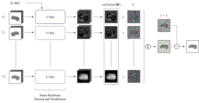
Figure 1: Architecture Overview. An arbitrary number of unordered and pose-free views coupled with the noise at timestep $t-1$ is denoised in parallel using the U-Net conditioned on timestep $t$ and target viewing angle $\Delta\psi$. The model then produces noise predictions and corresponding weights $w_{i}$ for timestep $t$. A composed noise prediction, computed as a weighted sum of individual contributions, is then subtracted from the previous timestep prediction. Ultimately, after $T$ timesteps, a fully denoised target view is obtained.

End-To-End Novel View Synthesis.

Using end-to-end based architectures is another commonly seen approach when it comes to novel view synthesis. For instance, Equivariant Neural Renderer (Dupont et al., 2020) aims to explicitly impose 3D structure on learned latent representations by ensuring that they transform like a real 3D scene. The encoded latents are then transformed before being passed to the decoder to produce the target view. Another example of an end-to-end approach that has shown promising performance for performing novel view synthesis is the Scene Representation Transformers (Sajjadi et al., 2022b) and its pose-free (Sajjadi et al., 2023) and object-centric (Sajjadi et al., 2022a) follow-ups. They focus on learning a latent representation of a scene by encoding a set of input images and passing it to a decoder in order to synthesise new views. A major drawback of the mentioned methods is their entirely deterministic nature, i.e. at inference time, they do not have the ability to output a variety of plausible views when dealing with underdetermined scenarios, making them difficult to use in the settings such as severe occlusion or limited amount of input views. (Sun et al., 2018) deal with this issue by employing a generative approach and self-learned confidence, but like the aforementioned NeRFs they require explicit pose information to be provided for each of the input views.

Diffusion Probabilistic Models.

Recently, models based on finding the reverse Markov chain transitions in order to maximize the likelihood of the training data, also known as diffusion probabilistic models (Sohl-Dickstein et al., 2015), have seen extensive use for solving various text-conditioned generative tasks (Ho et al., 2020; Rombach et al., 2022; Poole et al., 2022). This is due to their capabilities to produce high quality outputs when conditioned on textual descriptions. These models consist of a stochastic diffusion process and a deep neural network that parameterizes the denoising function used to perform the denoising procedure. Besides being used for generating images conditioned on text-based prompts, diffusion probabilistic models have seen applications in solving various other problems, including novel view synthesis. These range from models that use pre-trained stable diffusion backbones such as (Liu et al., 2023), to models trained from scratch such as (Müller et al., 2023), which operates directly on 3D radiance fields or (Watson et al., 2022), in which a novel view diffusion based model is introduced to perform end-to-end novel view synthesis in image domain. While these methods provide good qualitative results, they often come with various drawbacks. In particular, approaches based on using a pre-trained backbone rely on those backbones being freely and easily available. This is often not the case as authors of large models trained on extensive datasets refrain from making the weights and architectures publicly available, and instead provide access solely through an API, e.g. LLMs, large-scale diffusion models, etc. Furthermore, (Müller et al., 2023) lacks the ability to generalize across multiple classes, and (Watson et al., 2022) cannot make use of additional views when they are available. Therefore, even though they offer high quality synthesized views, they remain quite inflexible once trained.

3 Method

Our approach (Figure 1) employs a composable diffusion probabilistic framework in order to generate novel views. The model receives an unordered, pose-free and arbitrarily long collection of input views $\{\mathbf{x}_{i}\}_{i=1}^{N}$ of a given scene along with the target viewing direction $\Delta\psi$. The model then predicts the scene as viewed from the target viewing direction $\Delta\psi$.

3.1 Architecture

Each input view is treated separately through identical streams.

We feed each input view separately to an identical copy of the denoising backbone of a diffusion model (see Appendix A for a technical description of diffusion). We use a U-Net as the denoising backbone, with the same architecture and hyperparameters as (Saharia et al., 2022), unless specified otherwise below. Given a variable set of input views $\{\mathbf{x}_{i}\in\mathbb{R}^{3\times\textrm{H}\times\textrm{W}}\}_{i=1}^{N}$ we concatenate the noisy image at timestep $t$, $\{\textbf{y}_{t}\in\mathbb{R}^{3\times\textrm{H}\times\textrm{W}}\}_{t=1}^{T}$, along the channel dimension to each of the views, in order to produce a collection of U-Net inputs $\{V_{i}\in\mathbb{R}^{6\times\textrm{H}\times\textrm{W}}\}_{i=1}^{N}$, following (Saharia et al., 2022). Additionally, in order to globally condition the model on the target pose information, positional encodings (Vaswani et al., 2017) of the target pose $\Delta\psi$ (single angle in radians) and timestep $t$ (integer) are concatenated and jointly embedded using a simple MLP consisting of two layers – one hidden layer with a $sigmoid$ non-linearity followed by an output linear layer (dimensionality 128). The conditional embeddings produced by the MLP are injected into the U-Net through feature-wise affine transformations (Perez et al., 2018) in all downscaling and upscaling ResNet blocks. $\Delta\psi$ is the angular disparity between the target view and the canonical pose of the object, i.e. the front facing view of the object as defined in the dataset. We introduce the notation $\mathbf{c}_{i}^{t}\coloneqq(\mathbf{x}_{i},\mathbf{y}_{t},\Delta\psi,t)$ to denote a tuple containing all the inputs to the U-Net.

At each denoising step, all streams are composed through an inferred weighting strategy.

For a set of input views $\{\mathbf{x}_{i}\in\mathbb{R}^{3\times\textrm{H}\times\textrm{W}}\}_{i=1}^{N}$, a set of corresponding noise weighting masks $\{w_{i}\in\mathbb{R}^{3\times\textrm{H}\times\textrm{W}}\}_{i=1}^{N}$ is produced at every timestep by the U-Net backbone. Indeed, the U-Net outputs pairs of noise predictions $\hat{{\boldsymbol{\epsilon}}}_{i}$ and weights $w_{i}$, computed by two different heads at the final layer of the U-Net (obtained by changing the output layer channel count from 3 in the standard backbone to 6), each of the same dimensionality as the noise prediction (same dimension as the image). The weights are then stacked together into a tensor $\textbf{W}\in\mathbb{R}^{3N\times\textrm{H}\times\textrm{W}}$ and normalized using softmax along the first dimension. Next, these normalized weights are applied to the noise, and the weighted noise contributions are then summed, forming the final noise prediction $\mathbf{y}_{t-1}$. Intuitively, the weights reflect per-pixel informativeness of each of the input views for producing the target view. The described architecture is trained end-to-end using an $L_{2}$ loss computed between the true noise and model’s prediction. Algorithm 1 shows the training procedure pseudocode. $\alpha_{t}$ denotes the noise schedule and $\gamma_{t}=\prod_{t^{\prime}}^{t}\alpha_{t}^{{}^{\prime}}$, further described in Appendix A.

Algorithm 1 Composing View Contributions - Training

1:  repeat

2:    $(\mathbf{x},\Delta\psi,\mathbf{y}_{0})\sim q(\mathbf{x},\Delta\psi,\mathbf{y})$ {sample a datapoint}

3:    $t\sim\mathrm{Uniform}(\{1,\dotsc,T\})$ {sample a timestep}

4:    ${\boldsymbol{\epsilon}}\sim\mathcal{N}(\mathbf{0},\mathbf{I})$ {sample noise}

5:    $\hat{{\boldsymbol{\epsilon}}},\mathbf{W}\leftarrow f_{\theta}(\mathbf{x},\sqrt{\gamma_{t}}\mathbf{y}_{0}+\sqrt{1-\gamma_{t}}{\boldsymbol{\epsilon}},\Delta\psi,\gamma_{t})$ {predict the noise and weights}

6:    $w_{i}=\textit{softmax}(\mathbf{W},\text{dim=0})_{i}$ {normalize the weights}

7:    Take gradient descent step on

8:    $\qquad\nabla_{\theta}\left\|{\boldsymbol{\epsilon}}-\sum_{i=1}^{n}w_{i}\circ\hat{{\boldsymbol{\epsilon}}_{i}}\right\|^{2}$

9:  until converged

At inference time (Algorithm 2), the denoising process is repeated for $T$ timesteps. Like in training, after each timestep, the noise predictions are weighted and summed together. Then, they are passed as conditioning for the next timestep prediction. Ultimately, after $T$ timesteps, the final target view is produced.

Algorithm 2 Composing View Contributions - Inference

1:  $\mathbf{y}_{T}\sim\mathcal{N}(\mathbf{0},\mathbf{I})$ {sample starting noise}

2:  for $t=T,\dots,1$ do

3:    $\mathbf{z}\sim\mathcal{N}(\mathbf{0},\mathbf{I})$ if $t>1$, else $\mathbf{z}=\mathbf{0}$ {sample noise}

4:    $\hat{{\boldsymbol{\epsilon}}},\mathbf{W}\leftarrow f_{\theta}(\mathbf{x},\mathbf{y}_{t},\Delta\psi,\gamma_{t})$ {predict the noise and weights}

5:    $w_{i}=\textit{softmax}(\mathbf{W},\text{dim=0})_{i}$ {normalize the weights}

6:    $\mathbf{y}_{t-1}=\frac{1}{\sqrt{\alpha_{t}}}\left(\mathbf{y}_{t}-\frac{1-\alpha_{t}}{\sqrt{1-\gamma_{t}}}\sum_{i=1}^{n}w_{i}\circ\hat{{\boldsymbol{\epsilon}}_{i}}\right)+\sqrt{1-\alpha_{t}}\mathbf{z}$

7:  end for

8:  return $\mathbf{y}_{0}$

3.2 A Probabilistic Interpretation of ViewFusion

Here we provide a theoretical framework to justify the design choices of ViewFusion (see Appendix C for an extended version of this argument). We will do so by enforcing specific desiderata about the transition probability of the reverse diffusion process, in the specific context of pose-free novel view synthesis. First, given a set of input views $\{\mathbf{x}_{i}\}_{i=1}^{N}$, the transition probability of the reverse diffusion process should not depend on the specific order in which these input views are fed to the model. Indeed, input views do not contain pose information, and thus cannot be ordered in any meaningful way. One way to enforce such permutation invariance is to write the transition probability of the reverse diffusion process as a sum of contributions for each of the input views, where each input view contributes separately through an identical energy function $E$:

$$p(\mathbf{y}_{t-1}|\mathbf{c}^{t})\propto\sum_{i=1}^{N}\exp(-E(\mathbf{y}_{t-1},\mathbf{c}_{i}^{t})).$$ (1)

This functional form is permutation-invariant by construction (as also remarked by Zaheer et al. (2017)), hence it does not depend on the order of the $N$ input views. In addition, this functional form can be applied to any number of views, allowing our model to flexibly deal with an arbitrary number of views. This functional form can also be interpreted as a mixture of experts, where each individual view-conditioned-stream acts as one expert in predicting the reverse diffusion process.

Next, we show how the softmax weighting scheme in our approach directly derives from the functional form described above, without any further assumption. The update step of a diffusion model is given by the score (Song et al., 2020b):

$$\nabla_{\mathbf{y}}\log p(\mathbf{y}_{t-1}|\mathbf{c}^{t}).$$ (2)

By replacing $p$ with the functional form proposed in equation 1, we show (derivation in Appendix C) that the score reduces to:

$$\nabla_{\mathbf{y}}\log p(\mathbf{y}_{t-1}|\mathbf{c}^{t})=\sum_{i=1}^{N}w_{i}\nabla_{\mathbf{y}}(-E(\mathbf{y}_{t-1},\mathbf{c}_{i}^{t})),$$ (3)

where $w_{i}$ are the softmaxes over the energies $E_{i}$. This functional form for the update step is directly identifiable to the one we are using in our model, where (1) the weighting masks produced by our model correspond to the respective $w_{i}$, and (2) the predicted noise for each view-dependant stream corresponds to its respective view-dependant score $\nabla_{\mathbf{y}}(-E(\mathbf{y}_{t-1},\mathbf{c}_{i}^{t}))$. With this equivalence, we establish that the parallel stream architecture of ViewFusion, combined with its softmax aggregation scheme, derives directly from reasonable assumptions on the functional form of the transition probability of the reverse diffusion process, namely that it should be view-permutation-invariant, and more specifically that it should combine view-conditioned-predictions through a mixture of experts model.

4 Experimental Results

We evaluate our method on a relatively small, but diverse dataset, NMR, consisting of a variety of scenes and spanning multiple classes. We show that our model is capable of handling a wide variety of settings, while offering performances near or above the current state-of-the-art.

4.1 Dataset

Neural 3D Mesh Renderer Dataset (NMR).

NMR has been used extensively in previous work (Lin et al., 2023; Sajjadi et al., 2022b; Yu et al., 2021; Sitzmann et al., 2021) and serves as a good benchmark while keeping the computational footprint relatively low. The dataset is based on 3D renderings provided in (Kato et al., 2018). and consists of 13 classes (sofa, airplane, lamp, telephone, vessel, loudspeaker, chair, cabinet, table, display, car, bench, rifle) from ShapeNetCore (Chang et al., 2015) that were rendered from 24 azimuth angles (rotated around the vertical axis) at a fixed elevation angle using the same camera and lighting conditions. The resolution of each image is $64\times 64$. In total there are 44 k different objects, split across training, validation and testing sets as follows: 31 k, 4 k, 9 k. There are no overlaps in individual objects between the sets.

4.2 Evaluation Procedure

In order to ensure good generalization performance across a multitude of classes as well as variable input view count, we train a model by randomly picking the number of views that the model receives as conditioning, while training simultaneously across all the available classes. At evaluation time we test our model both in fixed-view as well as variable view settings. Implementation details as well as training configurations are available in Section B.1, and the full evaluation procedure is described in Section B.2.

We limit the model to receive anywhere between one and six views at random during the training, since providing an abundance of views can make the problem overly easy and completely determined while also requiring significant increase in computing power to process all of the views. However, even though we limit the training and inference to only up to six views, we also show that our approach is capable of generalizing to an arbitrary, previously unseen view counts.

NB All the evaluations were performed on a single model limited to receiving between one and six views at random during training time.

4.3 Quantitative Results

Table 2: Quantitative Results - Comparison of evaluated metrics against state-of-the-art models for NMR. NB To ensure equivalence of the results when comparing against SRT and ViT for NeRF, our model is restricted to receiving only a single input view at evaluation time. See Section B.2 for full evaluation procedure.

	$\uparrow$PSNR	$\uparrow$SSIM	$\downarrow$LPIPS
LFN (Sitzmann et al., 2021)	24.95	0.870	-
PixelNeRF (Yu et al., 2021)	26.80	0.910	0.108
SRT (Sajjadi et al., 2022b)	27.87	0.912	0.066
ViT for NeRF (Lin et al., 2023)	28.76	0.933	0.065
ViewFusion (Ours) - single view	26.0	0.883	0.053
1-4 ViewFusion (Ours) - up to six	29.03	0.925	0.033

We evaluate our model (Section 4.3) both in single-view and variable-view settings on commonly used metrics for novel view synthesis, namely PSNR, SSIM (Wang et al., 2004) and LPIPS (Zhang et al., 2018), and compare it to the most recent methods for novel view synthesis.

In order to ensure equivalence, we constrain our model to receiving only a single input view. This is effectively equivalent to turning off our learned weighting mechanism since all the weights scale to one after applying softmax. Even in this constrained scenario, our approach is able to reach state-of-the-art performance in LPIPS when compared to the previous approaches.

Additionally, we compute the metrics on the same model for the setting where it receives anywhere between one and six views as input conditioning at random. By doing so, we reach an even better state-of-the-art result in LPIPS, outperforming the current best approaches, and on par with state-of-the-art when it comes to PSNR and SSIM. This goes to show that our model is capable of effectively utilizing the availability of additional views. Better LPIPS results can be attributed to the fact that our model does not produce blur in areas of uncertainty (e.g. occluded areas) thanks to its generative capabilities, unlike prior methods, which often suffered from blurry results when producing areas of uncertainty (Sitzmann et al., 2021; Yu et al., 2021; Sajjadi et al., 2022b). LPIPS also more accurately reflects human perception than the other two metrics.

4.4 Qualitative Results

In order to underline the flexibility of our approach, we subject it to a variety of different scenarios (Table 1).

Variable Input Length.

One of the main advantages of our approach is the ability to effectively make use of a variable input view count both during inference and training. Figure 2 shows that we are consistently able to produce high quality samples regardless of the input view count. Additionally, thanks to the model being class agnostic, we use a single model to produce the results across all of the classes.

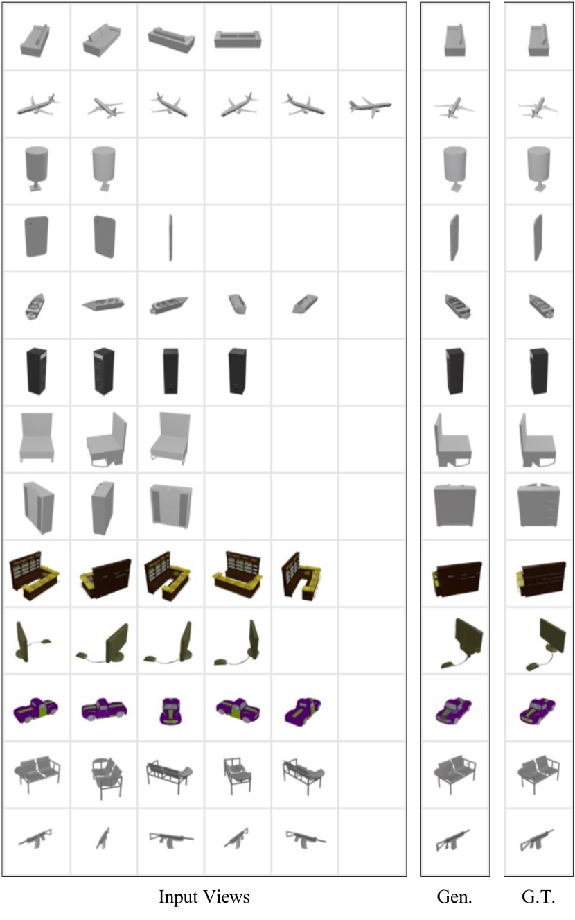
Figure 2: Variable Input Length. Our approach is capable of generalizing across different classes without re-training. The padded empty views are included for visualization purposes only and are not present during training or inference, as the model operates with an pose-free and unordered view collection of variable length within the batches.

Adaptive Weight Shifting.

By altering the target viewing direction, we show that the model shifts the weighting adaptively according to the informativeness of the input views that are provided (Figure 3). This weighting strategy allows the model to perform well even in scenarios where less informative views are given, that could normally act as a distraction. In Figure 3, we note that the views closest to the target view are selected by the weights, in accordance with our intuition that these views are most informative about the target view.

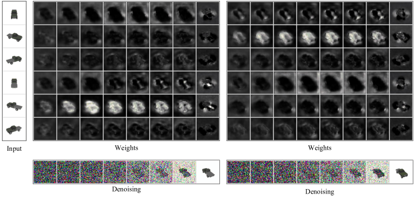
Figure 3: Adaptive Weight Shifting. The model shifts its weighting adaptively based on the most informative input view w.r.t. the desired target output. Six evenly spaced out views of the truck are passed in, depending on the target view the model puts most emphasis on the closest views. Additionally, it picks up on details from different views, e.g. the cargo bed and the back window of the truck are picked up from the fully rear facing input view in the first example or the front hull area in the second example that gets picked up from the front facing input view.

Severe Occlusion.

Due to the generative nature of our approach, the model is capable of producing several plausible views when required to generate target views viewed from a direction that is occluded in the input views. Figure 4 shows outputs of the model conditioned on the same input view and diverse starting noise, reflecting scenarios where the parts of the object present in the target view are heavily occluded in the input view.

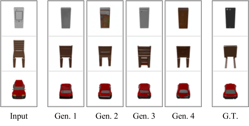
Figure 4: Severe Occlusion. Our approach is able to handle severely underdetermined settings by generating a variety of plausible view in cases where the target viewing direction is fully occluded. In this setting, we prompted the model with the same front views several times to generate plausible rear views.

Autoregressive 3D Consistency.

Despite not imposing any explicit 3D consistency constraints, in Figure 5 we show that our approach is capable of maintaining 3D consistency through autoregressive generation even when primed solely with a single input view. We start by priming the model with a single input view, and incrementally rotate the target viewing direction to produce novel views. During the autoregressive generation, we fully utilize the flexible context length by adding each consecutively generated view to the conditioning for producing the next view. By doing so, we ensure that the model is 3D consistent with itself. Additionally, unlike the previous approaches which often suffer from error accumulations by the time they reach the last frame, our model only elicits significant dissimilarities to the target when producing fully occluded parts (i.e. half way through the generative loop), which can not possibly be inferred from the initial input. This is due to the adaptive weighting which puts more weight back on the initial view past the midpoint of generation, ensuring that the produced samples are consistent start to end.

Figure 5: Autoregressive 3D Consistency. Our approach is capable of maintaining 3D consistency through autoregressive generation even when primed solely with a single input view. We start by priming the model with a single input view, and incrementally rotate the target viewing direction to produce novel views. During the autoregressive generation, each consecutively generated view is added to the flexible conditioning for producing the next view.

Generalization to Unseen View Counts.

The novel learnable weighting mechanism for composing the view contributions scales seamlessly to an arbitrary number of views that is even larger than the maximum presented during the training. In Figure 6, we show that our model trained on up to six views sensibly extrapolates even when presented with collections consisting of upwards of 20 views. Even though the problem is clearly determined with that many views, it is important to note that the model is able to sensibly compose them without its performance deteriorating.

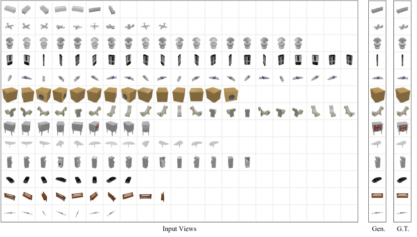
Figure 6: Generalization to Unseen View Counts. In addition to taking arbitrary number of input views, the model performs exceptionally well even when presented with significantly more input views at inference compared to the maximum of six at training time. Here we condition our model trained on up to six views on a significantly larger number of views.

5 Applications

This section explores potential application scenarios of ViewFusion based on the findings of this work.

Generating 3D Representations.

As shown previously in Section 4.4, our model is capable of autoregressively synthesizing a view of an object from all sides given only a single input view. This could be useful for a wide variety of VR or AR applications, as well as when trying to build a 3D representation of an object based on one or few images (e.g. for creating video game assets).

Occlusion Prediction.

Generative capabilities of our model could be leveraged to generate multiple plausible views of an occluded object. This can be particularly useful in situations where any kind of plausible view is needed, even if it might not be ground truth, or in scenarios where the absolute correctness of the produced views is not of significant importance.

Dataset Augmentation.

Lastly, recent findings (Abbas & Deny, 2023) have shown that commonly used deep networks for image classification fail to classify objects correctly when they are presented in unusual poses (e.g. flipped upside down or rotated in the 3D space). Therefore, our approach could be leveraged to further augment the already existing datasets used to train large classifiers, with the goal of improving their performance in a wide variety of edge-cases.

6 Limitations and Future Work

Our current approach does not explicitly incorporate 3D semantics of the scene. This can pose a problem in situations where a quick, on-the-fly adaptation to a completely new, out-of-distribution scene is needed. Another limitation is the trade-off between the generative power in underdetermined settings and the inference times for producing novel views, which scale linearly with the view count. This can make the model particularly slow when presented with a significant amount of input views or if the image resolution is significantly increased, especially when operating in an autoregressive mode. A potential way of fixing this would be to incorporate a well-established approach of performing diffusion in a latent space (Rombach et al., 2022) instead of image space. To further increase the inference speed, a DDIM (Song et al., 2020a) sampling strategy could be employed instead of DDPM. Furthermore, our method does not explicitly impose constraints to ensure 3D consistency due to the stochastic nature of diffusion modelling. However, this can be partly alleviated by using auto-regressive generation where each new view is also conditioned on previously generated views. Lastly, we test our model on a fairly limited and small NMR dataset. Therefore, in order to unleash the full potential of our generative approach and in order to enable it to operate in real-world scenarios, training on a more realistic and larger dataset would be required.

7 Conclusion

This work introduces ViewFusion, a flexible, pose-free generative approach for performing novel view synthesis using composable diffusion models. We propose a novel weighting scheme for composing diffusion models ensuring that only the most informative input views are taken into account for prediction of the target view, and enabling ViewFusion to adaptively handle an arbitrarily long and unordered collection of input views without the need to re-train. Additionally, the generative nature of ViewFusion enables it to generate plausible views even in severely underdetermined conditions. We believe that our approach serves as a valuable contribution when it comes to novel view synthesis, with a potential of being applied to other problems as well.

Acknowledgements

This work has been supported by a Helsinki Institute for Information Technology (HIIT) grant to B.S., and an Academy of Finland (AoF) grant to S.D. under the AoF Project: 3357590. We would like to extend our gratitude to Aalto Science-IT project for providing the computational resources and technical support.

Impact Statement

We provide a brief discussion on potential impacts and considerations that our approach entails.

Applications.

As already outlined in Section 5, we believe that our generative model can be used for a wide variety of purposes, such as various VR and AR applications, as well as when building 3D models of objects given one or few images.

Fake Content.

This paper proposes a generative method, which could potentially be used to produce images containing fake or misleading content. We believe that given the relatively small scale of our current model, this poses no immediate threat. However, in a scenario where the approach would be expanded to a significantly larger or a more realistic datasets, the risks would be mitigated by using the model in a controlled environment.

Energy Consumption.

We propose a method that requires a training procedure which can be computationally expensive, particularly if applied to a larger dataset than NMR. Additionally, our current sampling procedure can require significant amount of computing power, especially if a large collection of views is used as conditioning. Despite the potential computational footprint of our solution, our method offers unparalleled flexibility without the need to re-train. Therefore, we believe that it still remains reasonably efficient, as training is by far the most expensive part of the procedure.

Appendix A Diffusion Probabilistic Models

In this appendix we briefly introduce the technicalities of vanilla diffusion probabilistic models (Ho et al., 2020) based on (Saharia et al., 2022) and using the same notations as in the rest of the paper, but without the modifications introduced in Section 3.

Diffusion probabilistic models consist of a forward diffusion process during training and a corresponding reverse denoising process at the inference time. The forward process consists of gradually adding Gaussian noise to the image over $T$ timesteps, which can be described as following:

$$p(\textbf{y}_{t}|\textbf{y}_{t-1})=\mathcal{N}(\textbf{y}_{t};\sqrt{\alpha_{t}}\textbf{y}_{t-1},(1-\alpha_{t})I)$$ (4)

$$p(\mathbf{y}_{1:T}|\mathbf{y}_{0})=\prod_{t=1}^{T}q(\mathbf{y}_{t}|\mathbf{y}_{t-1})$$ (5)

where $\alpha_{t}$ is the noise schedule hyper-parameter. The noise is added up to a point where it is impossible to tell $\mathbf{y}_{t}$ from the Gaussian noise. The forward process at each step can also be marginalized as:

$$p(\textbf{y}_{t}|\textbf{y}_{0})=\mathcal{N}(\textbf{y}_{t};\sqrt{\gamma_{t}}\textbf{y}_{0},(1-\gamma_{t})I)$$ (6)

where $\gamma_{t}=\prod_{t^{\prime}}^{t}\alpha_{t}^{{}^{\prime}}$. By applying Gaussian parametrization of the forward process, we obtain a closed form formulation of the posterior distribution of $\textbf{y}_{t-1}$ given $(\textbf{y}_{0},\textbf{y}_{t})$:

$$p(\mathbf{y}_{t-1}|\textbf{y}_{0},\textbf{y}_{t})=\mathcal{N}(\textbf{y}_{t-1}|\boldsymbol{\mu},\sigma^{2}\textit{{I}})$$ (7)

in which $\boldsymbol{\mu}=\frac{\sqrt{\gamma_{t-1}}(1-\alpha_{t})}{1-\gamma_{t}}\mathbf{y}_{0}+\frac{\sqrt{\alpha_{t}}(1-\gamma_{t-1})}{1-\gamma_{t}}\mathbf{y}_{t}$ and $\sigma^{2}=\frac{(1-\gamma_{t-1})(1-\alpha_{t})}{1-\gamma_{t}}$. Having defined all the necessary aspects to perform diffusion, we can separate it into the training and inference procedures. During the training, the model acts as a denoising function and learns to invert the forward process. That means that given the noisy image $\mathbf{\tilde{y}}$, defined as

$$\mathbf{{\tilde{y}}}=\sqrt{\gamma}\mathbf{y}_{0}+\sqrt{1-\gamma}\boldsymbol{\epsilon},\;\boldsymbol{\epsilon}\sim\mathcal{N}(0,\textit{{I}})$$ (8)

the goal is to recover the original, target image $\mathbf{y}_{0}$. Therefore, the deep neural network model is parameterized as $f_{\theta}(\mathbf{x},\mathbf{\tilde{y}},\gamma)$, meaning it is conditioned on the input $\mathbf{x}$, a noisy image $\mathbf{\tilde{y}}$, and the noise level at a given time-step $\gamma$. The objective of the training procedure is to maximize a weighted variational-lower bound on the likelihood (Ho et al., 2020) and is given by

$$\mathbb{E}_{(\mathbf{x},\mathbf{y})}\mathbb{E}_{\epsilon,\gamma}\Big{\|}f_{\theta}(\mathbf{x},\underbrace{\sqrt{\gamma}\mathbf{y}_{0}+\sqrt{1-\gamma}\boldsymbol{\epsilon}}_{\mathbf{\tilde{y}}},\gamma)-\boldsymbol{\epsilon}\Big{\|}_{p}^{p}.$$ (9)

Pseudocode for the training procedure is given in Algorithm 3.

Algorithm 3 Training - Forward (Noising) Process

1:  repeat

2:    $(\mathbf{x},\mathbf{y}_{0})\sim q(\mathbf{x},\mathbf{y})$

3:    $t\sim\mathrm{Uniform}(\{1,\dotsc,T\})$

4:    ${\boldsymbol{\epsilon}}\sim\mathcal{N}(\mathbf{0},\mathbf{I})$

5:    Take gradient descent step on

6:    $\qquad\nabla_{\theta}\left\|f_{\theta}(\mathbf{x},\sqrt{\bar{\alpha}_{t}}\mathbf{y}_{0}+\sqrt{1-\gamma_{t}}{\boldsymbol{\epsilon}},t)-{\boldsymbol{\epsilon}}\right\|^{2}$

7:  until converged

In order to perform inference, we want to perform a reverse process over $T$ iterative refinement steps, i.e. the goal is to go from a randomly sampled Gaussian noise back to the image by iterative denoising. In order to do so, we first need to approximate $\mathbf{y}_{0}$ by utilizing Equation 8 to obtain:

$$\hat{\mathbf{y}}_{0}=\frac{1}{\sqrt{\gamma_{t}}}\Big{(}\mathbf{y}_{t}-\sqrt{1-\gamma_{t}}f(\mathbf{x},\mathbf{y}_{t},\gamma_{t})\Big{)}.$$ (10)

Now we can substitute $\hat{\mathbf{y}}_{0}$ into $p(\mathbf{y}_{t-1}|\mathbf{y}_{0},\mathbf{y}_{t})$ from Equation 7 in order to parameterize the mean of $p_{\theta}(\mathbf{y}_{t-1}|\mathbf{y}_{t},x)$ as

$$\mu_{\theta}(\mathbf{x},\mathbf{y}_{t},\gamma_{t})=\frac{1}{\sqrt{\alpha_{t}}}\Big{(}\mathbf{y}_{t}-\frac{1-\alpha_{t}}{\sqrt{1-\gamma_{t}}}f_{\theta}(\mathbf{x},\mathbf{y}_{t},\gamma_{t})\Big{)}.$$ (11)

By setting the variance of $p_{\theta}(\mathbf{y}_{t-1}|\mathbf{y}_{t},\mathbf{x})$ to $(1-\alpha_{t})$, each step of the iterative reverse process can be computed as

$$\mathbf{y}_{t-1}\longleftarrow\frac{1}{\sqrt{\alpha_{t}}}\Big{(}\mathbf{y}-\frac{1-\alpha_{t}}{\sqrt{1-\gamma_{t}}}f_{\theta}(\mathbf{x},\mathbf{y}_{t},\gamma_{t})\Big{)}+\sqrt{1-\alpha_{t}}{\boldsymbol{\epsilon}}_{t}.$$ (12)

Pseudocode describing the inference procedure is given in Algorithm 4.

Algorithm 4 Inference - Reverse (Denoising) Process

1:  $\mathbf{y}_{T}\sim\mathcal{N}(\mathbf{0},\mathbf{I})$

2:  for $t=T,\dotsc,1$ do

3:    $\mathbf{z}\sim\mathcal{N}(\mathbf{0},\mathbf{I})$ if $t>1$, else $\mathbf{z}=\mathbf{0}$

4:    $\mathbf{y}_{t-1}=\frac{1}{\sqrt{\alpha_{t}}}\left(\mathbf{y}_{t}-\frac{1-\alpha_{t}}{\sqrt{1-\gamma_{t}}}f_{\theta}(\mathbf{x},\mathbf{y}_{t},\gamma_{t})\right)+\sqrt{1-\alpha_{t}}\mathbf{z}$

5:  end for

6:  return $\mathbf{y}_{0}$

Appendix B Implementation Details

B.1 Architecture and Hyperparameters

We base our U-Net architecture on (Saharia et al., 2022) with modifications listed in Section 3.1. Following (Karras et al., 2022), a linear noise scheduling is applied for the diffusion process spanning (1e-6, 0.01) over 2000 timesteps, both for training and inference.

We train the model on $L_{2}$ loss computed between the loss prediction and true noise. Furthermore, a learning rate scheduler is used in combination with Adam optimizer. The learning rate starts at 5e-5 with a 10k steps as a warm-up following which it peaks at 1e-4. We train the model, conditioned on one to six input views, for 710k steps using a batch size of 112 and 4$\times$V100 GPUs. The total training time using this setup amounts to approximately 6.5 days.

Listing 1 shows PyTorch pseudocode for aggregating the view contributions at each diffusion step, given an arbitrary, unordered and pose-free collection of input views.

B.2 Evaluation Details

In order to ensure consistency of our evaluation process given the stochastic generative nature of our model, and while maintaining a reasonably low computational footprint, we repeat the evaluation procedure several times using the same model. For single-view setting, we evaluate the same model three times over the whole test dataset, by randomly picking an input view and an arbitrary target for each object. subsection 4.3 reports the mean metrics of this procedure. We omit reporting standard deviations directly in Section 4.3 as they are orders of magnitudes lower than the metrics themselves, namely $\pm$3.18e-2 for PSNR, $\pm$4.78e-4 for SSIM and $\pm$1.41e-4 for LPIPS, respectively. We perform a single run where the model receives up to six views, as it is significantly more expensive than the single-view setting and its results cannot be directly compared to prior methods.

It is important to note that this differs slightly from evaluation procedures of (Sajjadi et al., 2022b; Lin et al., 2023) where for a randomly picked input view, all other 23 views are generated. We avoid performing this procedure as we observe stable results are already obtained from the separate runs, as well as to maintain a low computational footprint as our sampling procedure can take a significant amount of time to be computed over the whole dataset.

Listing 1 PyTorch Pseudocode for Contribution Aggregation

⬇

1

2# create delimiter indices for unstacking the U-Net outputs

3# view_count of shape (B, 1) - number of input views for each sample in the batch

4view_delimiters = torch.cumsum(view_count, 0).tolist()

5view_delimiters.insert(0, 0)

6

7noise_level = extract(self.gammas, t, x_shape=(1, 1)).to(y_t.device)

8

9# prepare shapes of conditioning, noise, angles and levels;

10# from (B, 23, C, H, W) -> ((V_1 + ... + V_B), C, H, W); where v_n is the input view count for each sample

11x_stacked = torch.concatenate(

12 [x_i[i, :idx] for i, idx in enumerate(view_count)],

13 dim=0,

14).to(x_i.device)

15

16y_t_stacked = torch.repeat_interleave(y_t, view_count, dim=0)

17noise_level_stacked = torch.repeat_interleave(noise_level, view_count, dim=0)

18angle_stacked = torch.repeat_interleave(angle, view_count, dim=0)

19

20unet_output = self.unet(

21 torch.cat([x_stacked, y_t_stacked], dim=1),

22 angle_stacked,

23 noise_level_stacked,

24)

25noise_all, logits = unet_output[:, :3, ...], unet_output[:, 3:, ...]

26

27# weights and noise padded; shape (B, max(V_1, ... , V_B), C, H, W)

28logits_padded = torch.nn.utils.rnn.pad_sequence(

29 [

30 logits[idx1:idx2]

31 for idx1, idx2 in zip(view_delimiters[:-1], view_delimiters[1:])

32 ],

33 batch_first=True,

34 padding_value=float("-inf"), # -inf padding becomes 0 after softmax

35)

36weights_softmax = F.softmax(logits_padded, dim=1)

37noise_padded = torch.nn.utils.rnn.pad_sequence(

38 [

39 noise_all[idx1:idx2]

40 for idx1, idx2 in zip(view_delimiters[:-1], view_delimiters[1:])

41 ],

42 batch_first=True,

43)

44noise_weighted = noise_padded * weights_softmax

45

46noise = noise_weighted.sum(dim=1)

Appendix C A Probabilistic Interpretation of ViewFusion

We hereby elucidate the design choices of the ViewFusion approach by means of a probabilistic interpretation. In the following, we will assume a specific expression for the transition probability of the reverse diffusion process, where we will recover a weighted composition of per-view noise gradients.

We use the following notation:

1. $\mathbf{y}_{t-1}$ and $\mathbf{y}_{t}$, the images produced by the diffusion process at times $t-1$ and $t$, respectively;

2. $t$ being the time variable;

3. $\{\mathbf{x}_{i}\}_{i=1}^{N}$ being the set of $N$ conditioning images, each detailing a different pose of the object of interest;

4. $\Delta\psi$ being the conditioning target angle.

For brevity, we contain all the conditional information in a tuple $\mathbf{c}_{i}^{t}\coloneqq(\mathbf{x}_{i},\mathbf{y}_{t},\Delta\psi,t)$.

We want to model the transition probability of the reverse diffusion process p(y_t-1— c^t). Since $\{\mathbf{x}_{i}\}_{i=1}^{N}$ is a set, the expression of the probability $p(\mathbf{y}_{t-1}|\mathbf{c}_{i}^{t})$ should not depend on the order of the conditioning images, nor on their number. We can consider a single function $E$ applied separately to each of the $N$ views, and have these terms contribute to the final probability via summation. In a formula, p(y_t-1— c^t) ∝∑_i=1^N exp(-E(y_t-1, c_i^t)). With this prescription, in accordance to (Zaheer et al., 2017), the probability is now a function that does not depend on the order of the $N$ views, and can be applied to any number of views (in their notation, we have $\phi=\exp(-E)$ and $\rho=\mathrm{Id}$). In the machine learning context, this formulation is sometimes referred to as a Mixture of Experts (MoE), where the experts here correspond to the different input views, and the output is the probability distribution of the reverse diffusion step. This is also known, in the context of physics, as a Boltzmann distribution. The analogy implies that the $N$ views act as states of the system, each of them with an associated energy, and the probability of each state is proportional to the exponential of the negative of this energy. These states then combine their influence on the reverse diffusion process paths via their summation.

We are now interested in the score, p(y_t-1— c^t) ∝∑_i=1^N exp(-E(y_t-1, c_i^t)). as this is the quantity which the model is trained to predict, following (Song et al., 2020b). We perform the computations directly:

$$\nabla_{\mathbf{y}}\log p(\mathbf{y}_{t-1}|\mathbf{c}^{t}) =\nabla_{\mathbf{y}}\log\sum_{i=1}^{N}\exp(-E(\mathbf{y}_{t-1},\mathbf{c}_{i}^{t}))$$ (13)

$$=\frac{\nabla_{\mathbf{y}}\sum_{i=1}^{N}\exp(-E(\mathbf{y}_{t-1},\mathbf{c}_{i}^{t}))}{\sum_{j=1}^{N}\exp(-E(\mathbf{y}_{t-1},\mathbf{c}_{i}^{t}))}$$ (14)

$$=\sum_{i=1}^{N}\frac{\nabla_{\mathbf{y}}\exp(-E(\mathbf{y}_{t-1},\mathbf{c}_{i}^{t}))}{\sum_{j=1}^{N}\exp(-E(\mathbf{y}_{t-1},\mathbf{c}_{i}^{t}))}$$ (15)

$$=\sum_{i=1}^{N}\frac{\exp(-E(\mathbf{y}_{t-1},\mathbf{c}_{i}^{t}))}{\sum_{j=1}^{N}\exp(-E(\mathbf{y}_{t-1},\mathbf{c}_{i}^{t}))}\nabla_{\mathbf{y}}(-E(\mathbf{y}_{t-1},\mathbf{c}_{i}^{t})),$$ (16)

where we recognise the softmax function. For ease of writing and reading, we call

$$w_{i}=\frac{\exp(-E(\mathbf{y}_{t-1},\mathbf{c}_{i}^{t}))}{\sum_{j=1}^{N}\exp(-E(\mathbf{y}_{t-1},\mathbf{c}_{i}^{t}))}.$$ (17)

Then

$$\nabla_{\mathbf{y}}\log p(\mathbf{y}_{t-1}|\mathbf{c}^{t})=\sum_{i=1}^{N}w_{i}\nabla_{\mathbf{y}}(-E(\mathbf{y}_{t-1},\mathbf{c}_{i}^{t})),$$ (18)

and so we recover the weighting of the contributions of each conditioning image.

While, in principle, knowledge of $E$ is enough to completely characterise $p$ (as each of the $w_{i}$ is expressible as a function of all the $N$ energies), in this work we predict separately the weights $w_{i}$ and the gradients of the energies (also called scores).

References

- Abbas & Deny (2023) Abbas, A. and Deny, S. Progress and limitations of deep networks to recognize objects in unusual poses. In Proceedings of the AAAI Conference on Artificial Intelligence, volume 37, pp. 160–168, 2023.
- Agarwal et al. (2011) Agarwal, S., Furukawa, Y., Snavely, N., Simon, I., Curless, B., Seitz, S. M., and Szeliski, R. Building rome in a day. Communications of the ACM, 54(10):105–112, 2011.
- Chang et al. (2015) Chang, A. X., Funkhouser, T., Guibas, L., Hanrahan, P., Huang, Q., Li, Z., Savarese, S., Savva, M., Song, S., Su, H., et al. Shapenet: An information-rich 3d model repository. arXiv preprint arXiv:1512.03012, 2015.
- Dupont et al. (2020) Dupont, E., Martin, M. B., Colburn, A., Sankar, A., Susskind, J., and Shan, Q. Equivariant neural rendering. In International Conference on Machine Learning, pp. 2761–2770. PMLR, 2020.
- Ho et al. (2020) Ho, J., Jain, A., and Abbeel, P. Denoising diffusion probabilistic models. Advances in Neural Information Processing Systems, 33:6840–6851, 2020.
- Karras et al. (2022) Karras, T., Aittala, M., Aila, T., and Laine, S. Elucidating the design space of diffusion-based generative models. Advances in Neural Information Processing Systems, 35:26565–26577, 2022.
- Kato et al. (2018) Kato, H., Ushiku, Y., and Harada, T. Neural 3d mesh renderer. In Proceedings of the IEEE conference on computer vision and pattern recognition, pp. 3907–3916, 2018.
- Kim et al. (2013) Kim, B.-s., Kohli, P., and Savarese, S. 3d scene understanding by voxel-crf. In Proceedings of the IEEE International Conference on Computer Vision, pp. 1425–1432, 2013.
- Lin et al. (2023) Lin, K.-E., Lin, Y.-C., Lai, W.-S., Lin, T.-Y., Shih, Y.-C., and Ramamoorthi, R. Vision transformer for nerf-based view synthesis from a single input image. In Proceedings of the IEEE/CVF Winter Conference on Applications of Computer Vision, pp. 806–815, 2023.
- Liu et al. (2023) Liu, R., Wu, R., Van Hoorick, B., Tokmakov, P., Zakharov, S., and Vondrick, C. Zero-1-to-3: Zero-shot one image to 3d object. arXiv preprint arXiv:2303.11328, 2023.
- Mildenhall et al. (2021) Mildenhall, B., Srinivasan, P. P., Tancik, M., Barron, J. T., Ramamoorthi, R., and Ng, R. Nerf: Representing scenes as neural radiance fields for view synthesis. Communications of the ACM, 65(1):99–106, 2021.
- Müller et al. (2023) Müller, N., Siddiqui, Y., Porzi, L., Bulo, S. R., Kontschieder, P., and Nießner, M. Diffrf: Rendering-guided 3d radiance field diffusion. In Proceedings of the IEEE/CVF Conference on Computer Vision and Pattern Recognition, pp. 4328–4338, 2023.
- Perez et al. (2018) Perez, E., Strub, F., De Vries, H., Dumoulin, V., and Courville, A. Film: Visual reasoning with a general conditioning layer. In Proceedings of the AAAI conference on artificial intelligence, volume 32, 2018.
- Poole et al. (2022) Poole, B., Jain, A., Barron, J. T., and Mildenhall, B. Dreamfusion: Text-to-3d using 2d diffusion. arXiv preprint arXiv:2209.14988, 2022.
- Riegler & Koltun (2020) Riegler, G. and Koltun, V. Free view synthesis. In Computer Vision–ECCV 2020: 16th European Conference, Glasgow, UK, August 23–28, 2020, Proceedings, Part XIX 16, pp. 623–640. Springer, 2020.
- Rombach et al. (2022) Rombach, R., Blattmann, A., Lorenz, D., Esser, P., and Ommer, B. High-resolution image synthesis with latent diffusion models. In Proceedings of the IEEE/CVF conference on computer vision and pattern recognition, pp. 10684–10695, 2022.
- Saharia et al. (2022) Saharia, C., Chan, W., Chang, H., Lee, C., Ho, J., Salimans, T., Fleet, D., and Norouzi, M. Palette: Image-to-image diffusion models. In ACM SIGGRAPH 2022 Conference Proceedings, pp. 1–10, 2022.
- Sajjadi et al. (2022a) Sajjadi, M. S., Duckworth, D., Mahendran, A., van Steenkiste, S., Pavetic, F., Lucic, M., Guibas, L. J., Greff, K., and Kipf, T. Object scene representation transformer. Advances in Neural Information Processing Systems, 35:9512–9524, 2022a.
- Sajjadi et al. (2022b) Sajjadi, M. S., Meyer, H., Pot, E., Bergmann, U., Greff, K., Radwan, N., Vora, S., Lučić, M., Duckworth, D., Dosovitskiy, A., et al. Scene representation transformer: Geometry-free novel view synthesis through set-latent scene representations. In Proceedings of the IEEE/CVF Conference on Computer Vision and Pattern Recognition, pp. 6229–6238, 2022b.
- Sajjadi et al. (2023) Sajjadi, M. S., Mahendran, A., Kipf, T., Pot, E., Duckworth, D., Lučić, M., and Greff, K. Rust: Latent neural scene representations from unposed imagery. In Proceedings of the IEEE/CVF Conference on Computer Vision and Pattern Recognition, pp. 17297–17306, 2023.
- Sitzmann et al. (2021) Sitzmann, V., Rezchikov, S., Freeman, B., Tenenbaum, J., and Durand, F. Light field networks: Neural scene representations with single-evaluation rendering. Advances in Neural Information Processing Systems, 34:19313–19325, 2021.
- Sohl-Dickstein et al. (2015) Sohl-Dickstein, J., Weiss, E., Maheswaranathan, N., and Ganguli, S. Deep unsupervised learning using nonequilibrium thermodynamics. In International conference on machine learning, pp. 2256–2265. PMLR, 2015.
- Song et al. (2020a) Song, J., Meng, C., and Ermon, S. Denoising diffusion implicit models. arXiv preprint arXiv:2010.02502, 2020a.
- Song et al. (2020b) Song, Y., Sohl-Dickstein, J., Kingma, D. P., Kumar, A., Ermon, S., and Poole, B. Score-based generative modeling through stochastic differential equations. arXiv preprint arXiv:2011.13456, 2020b.
- Sun et al. (2018) Sun, S.-H., Huh, M., Liao, Y.-H., Zhang, N., and Lim, J. J. Multi-view to novel view: Synthesizing novel views with self-learned confidence. In Proceedings of the European Conference on Computer Vision (ECCV), pp. 155–171, 2018.
- Vaswani et al. (2017) Vaswani, A., Shazeer, N., Parmar, N., Uszkoreit, J., Jones, L., Gomez, A. N., Kaiser, Ł., and Polosukhin, I. Attention is all you need. Advances in neural information processing systems, 30, 2017.
- Wang et al. (2004) Wang, Z., Bovik, A. C., Sheikh, H. R., and Simoncelli, E. P. Image quality assessment: from error visibility to structural similarity. IEEE transactions on image processing, 13(4):600–612, 2004.
- Watson et al. (2022) Watson, D., Chan, W., Martin-Brualla, R., Ho, J., Tagliasacchi, A., and Norouzi, M. Novel view synthesis with diffusion models. arXiv preprint arXiv:2210.04628, 2022.
- Yu et al. (2021) Yu, A., Ye, V., Tancik, M., and Kanazawa, A. pixelnerf: Neural radiance fields from one or few images. In Proceedings of the IEEE/CVF Conference on Computer Vision and Pattern Recognition, pp. 4578–4587, 2021.
- Zaheer et al. (2017) Zaheer, M., Kottur, S., Ravanbakhsh, S., Poczos, B., Salakhutdinov, R. R., and Smola, A. J. Deep sets. Advances in neural information processing systems, 30, 2017.
- Zhang et al. (2018) Zhang, R., Isola, P., Efros, A. A., Shechtman, E., and Wang, O. The unreasonable effectiveness of deep features as a perceptual metric. In Proceedings of the IEEE conference on computer vision and pattern recognition, pp. 586–595, 2018.