Bayesian Federated Inference for regression models
with heterogeneous multi-center populations

Abstract

To estimate accurately the parameters of a regression model, the sample size must be large enough relative to the number of possible predictors for the model. In practice, sufficient data is often lacking, which can lead to overfitting of the model and, as a consequence, unreliable predictions of the outcome of new patients. Pooling data from different data sets collected in different (medical) centers would alleviate this problem, but is often not feasible due to privacy regulation or logistic problems. An alternative route would be to analyze the local data in the centers separately and combine the statistical inference results with the Bayesian Federated Inference (BFI) methodology. The aim of this approach is to compute from the inference results in separate centers what would have been found if the statistical analysis was performed on the combined data. We explain the methodology under homogeneity and heterogeneity across the populations in the separate centers, and give real life examples for better understanding. Excellent performance of the proposed methodology is shown. An R-package to do all the calculations has been developed and is illustrated in this paper. The mathematical details are given in the Appendix.

Keywords: Bayesian analysis, data integration, Federated Learning, multi center data, prediction model

1 Introduction

Prediction models aim to predict the outcome of interest for individuals (or subjects), based on their values of the covariates in the model. To build a prediction model by selecting covariates and estimating the corresponding regression parameters, the sample size should be sufficiently large. If too many variables (possible covariates) relative to the number of events or observations are included, the model may become overly flexible and erroneously ‘explain’ noise or random variations in the data, rather than estimating meaningful relationships between the covariates and the outcome. This is called overfitting and may lead to unreliable predictions of the outcome for new individuals[1]. To overcome overfitting a minimum of 10 to 20 observations or events per variable (EPV) is often advised[2, 3]. Based on this criterion, data sets are often too small to take all available variables in consideration. Merging data sets from different (medical) centers could in principle alleviate the problem, but is often difficult for regulatory and logistic reasons. An alternative route would be to analyse the local data in the centers and combine the obtained inference results intelligently. With this approach the (individual) data do not need to be shared across centers.

Federated Learning (FL) is a machine learning approach that was developed several years ago, mainly for analyzing data from different mobile devices [4]. It aims to construct from the inference results obtained in the separate centers, what would have been found if the analysis was performed on the combined data set. With this approach, the local data stay at their owners’ centers, only parameter estimates are cycled around and updated based on the local data until a convergence criterion is met (see Figure 1, plot on the left). In recent years the FL approach has improved quite a bit [5] and may perform excellently in e.g. image analysis [6, 7, 8] or for data from mobile devises, but has clearly some drawbacks in other applications. For instance, apart from obvious ones such as data security and convergence problems, if one aims to estimate statistical models based on inference results from different medical centers, one needs to handle challenges like heterogeneity of the populations across centers, center specific covariates (like location), missing covariates in the data, and the fact that data may be stored in different ways (covariates are named differently or are even defined differently).

In this paper we describe the Bayesian Federated Inference (BFI) framework. BFI has the same aim as FL, but was developed especially for combining inference results from different centers to estimate statistical (regression) models without the need for repeated iterations. In every center the data are analysed only once and the inference results (parameter and accuracy estimates) are sent to a central server. At the central server the local inference results are combined to one single set of estimates in such a way that the obtained estimates are approximately equal to the estimates that would have been obtained had the data sets first combined before doing the analysis (see Figure 1, plot on the right). A cycling mechanism like for FL is not necessary. The mathematical theory of the BFI methodology was published by the authors in Jonker et al [9]. In this paper, we extend the theory further to allow for different kinds of heterogeneity across the centers. Furthermore, there is more focus on applications: a data example is given and the R code (from our R package BFI) for analyzing the data with the BFI methodology is explained.

This paper is organized as follows. In Section 2 the BFI framework for generalized linear models (GLMs) for homogeneous sub-populations is explained. In Section 3 different types of heterogeneity across sub-populations and data sets are described and it is explained how the BFI methodology can be adjusted to takes these into account. To study the performance of the BFI method in different settings, the results of simulation studies are described in Section 4. We explain how to do the analysis in Rstudio in Section 5. A discussion is given in Section 6 and the paper ends with an appendix that contains various mathematical details.

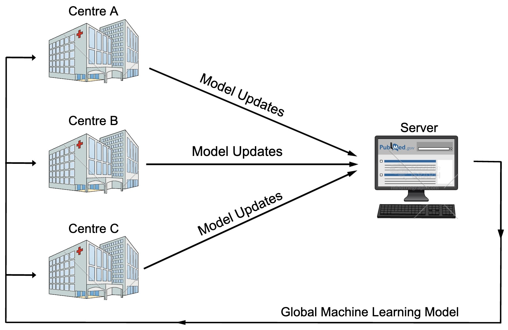
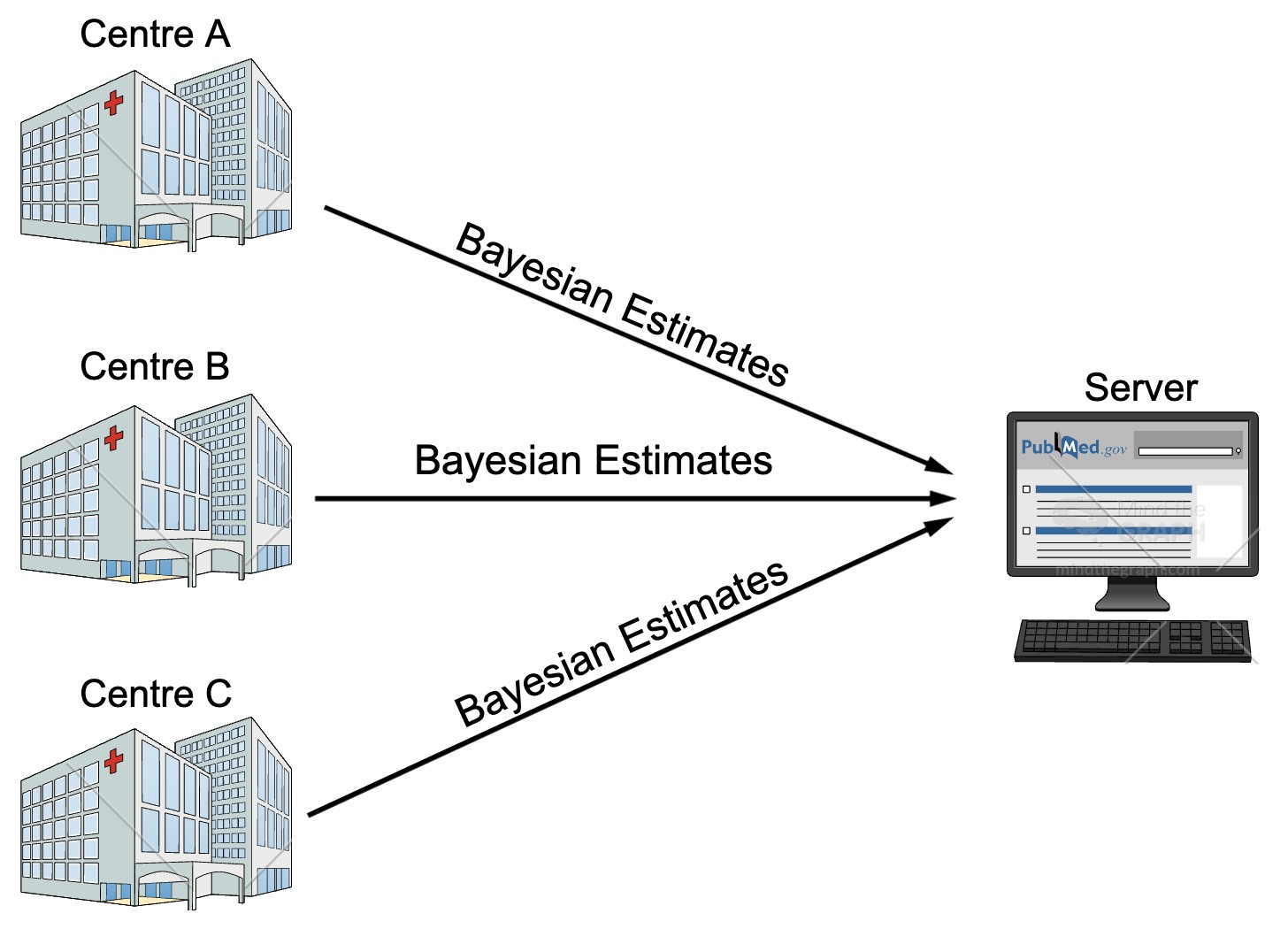
Figure 1: Visualisations of the Federated Learning cycling mechanism (left), and the Bayseian Federated Inference strategy (right). In both cases there are three local centers (A, B and C).

2 The Bayesian Federated Inference (BFI) framework

Suppose that data of $L$ medical centers are locally available, but these data-sets cannot be merged to a single integrated data-set for statistical analysis. The data for individual $i$ from center $\ell$ is denoted as the pair $({\bf x}_{\ell i},y_{\ell i})$ with ${\bf x}_{\ell i}$ a vector of covariates and $y_{\ell i}$ the outcome of interest. Let ${\bf D}_{\ell}$ denote the data subset in center $\ell$:

$${\bf D}_{\ell}=\{({\bf x}_{\ell 1},y_{\ell 1}),\ldots,({\bf x}_{\ell n_{\ell}},y_{\ell n_{\ell}})\},$$

where $n_{\ell}$ denotes the number of individuals in subset $\ell$, $\ell=1,\ldots,L$, and let ${\bf D}$ be the fictive combined data set (the union of the subsets ${\bf D}_{1},\ldots,{\bf D}_{L}$).

The data pair $({\bf x}_{\ell i},y_{\ell i})$ is the realisation of the stochastic pair $({\bf X}_{\ell i},Y_{\ell i})$. Suppose that the variables $({\bf X}_{\ell i},Y_{\ell i}),i=1,\ldots,n_{\ell},\ell=1,\ldots,L$ are independent and identically distributed, and that ${\bf X}_{\ell i}$ and $Y_{\ell i}$ are linked via a generalized linear model (GLM) with link function $h$:

$$h\big{(}\mathbb{E}(Y_{\ell i}|{\bf X}_{\ell i},\mbox{\boldmath$\mu$},\mbox{\boldmath$\beta$})\big{)}=\mbox{\boldmath$\beta$}^{t}{\bf X}_{\ell i},$$

where $\beta$ is a vector of unknown regression parameters and $\mu$ a vector of unknown nuisance parameters. If the first element in the covariate vector ${\bf X}_{\ell i}$ equals one for all individuals, the model includes an intercept.

For $\mbox{\boldmath$\theta$}_{1}:=(\mbox{\boldmath$\mu$},\mbox{\boldmath$\beta$})$, the conditional density of $Y_{\ell i}|({\bf X}_{\ell i}={\bf x},\mbox{\boldmath$\theta$}_{1})$ is given by $y|{\bf x},\mbox{\boldmath$\theta$}_{1}\to p(y|{\bf x},\mbox{\boldmath$\theta$}_{1})$ and for the vector of covariates ${\bf X}_{\ell i}|\mbox{\boldmath$\theta$}_{2}$ this is ${\bf x}|\mbox{\boldmath$\theta$}_{2}\to p({\bf x}|\mbox{\boldmath$\theta$}_{2})$, for $\mbox{\boldmath$\theta$}_{2}$ a parameter vector. Then, for $\mbox{\boldmath$\theta$}:=(\mbox{\boldmath$\theta$}_{1},\mbox{\boldmath$\theta$}_{2})$ it follows that the density of $y,{\bf x}|\mbox{\boldmath$\theta$}$ can be written as $y,{\bf x}|\mbox{\boldmath$\theta$}\to p(y,{\bf x}|\mbox{\boldmath$\theta$})\;=\;p(y|{\bf x},\mbox{\boldmath$\theta$}_{1})p({\bf x}|\mbox{\boldmath$\theta$}_{2})$. We work in a Bayesian setting; $\theta$ is stochastic as well. For mathematical simplicity, we assume statistical independence between $\mbox{\boldmath$\theta$}_{1}$ and $\mbox{\boldmath$\theta$}_{2}$. Thus, $p(\mbox{\boldmath$\theta$}_{1},\mbox{\boldmath$\theta$}_{2})=p(\mbox{\boldmath$\theta$}_{1})p(\mbox{\boldmath$\theta$}_{2})$ in the combined data set ${\bf D}$ and $p_{\ell}(\mbox{\boldmath$\theta$}_{1},\mbox{\boldmath$\theta$}_{2})=p_{\ell}(\mbox{\boldmath$\theta$}_{1})p_{\ell}(\mbox{\boldmath$\theta$}_{2})$ in center $\ell$, for all $\ell$ (the “$\ell$” in the subscript refers to the center). We choose the prior parameter distributions for $\mbox{\boldmath$\theta$}_{1}$ and $\mbox{\boldmath$\theta$}_{2}$ to be Gaussian with mean zero and inverse covariance matrices $\mbox{\boldmath$\Lambda$}_{1}$ and $\mbox{\boldmath$\Lambda$}_{2}$, respectively, in the combined data set, and $\mbox{\boldmath$\Lambda$}_{1,\ell}$ and $\mbox{\boldmath$\Lambda$}_{2,\ell}$ in center $\ell$, $\ell=1,\ldots,L$.

The maximum a posteriori (MAP) estimate of $\mbox{\boldmath$\theta$}=(\mbox{\boldmath$\theta$}_{1},\mbox{\boldmath$\theta$}_{2})$ maximizes the a posteriori density of the data with respect to $\theta$, by definition. For the combined data set ${\bf D}$, this estimate is denoted as $\widehat{\mbox{\boldmath$\theta$}}=(\widehat{\mbox{\boldmath$\theta$}}_{1},\widehat{\mbox{\boldmath$\theta$}}_{2})$ and, for the local data set ${\bf D}_{\ell}$ the notation $\widehat{\mbox{\boldmath$\theta$}}_{\ell}=(\widehat{\mbox{\boldmath$\theta$}}_{1,\ell},\widehat{\mbox{\boldmath$\theta$}}_{2,\ell})$ is used. If the prior density is chosen to be non-informative (large prior variances), the MAP-estimates will be close to the maximum likelihood estimates. The estimator $\widehat{}\mbox{\boldmath$\theta$}$ is fictive as the data set ${\bf D}$ can not be created. In the following we derive expressions for $\widehat{\mbox{\boldmath$\theta$}}$ in terms of the MAP estimators based on the local data sets ${\bf D}_{\ell}$. Once the estimates in the separate centers have been found, these expressions tell us how to combine them to obtain (an approximation of) $\widehat{\mbox{\boldmath$\theta$}}$.

For the fictive combined data set ${\bf D}$ the log posterior density can be written as

$$\log\big{\{}p(\mbox{\boldmath$\theta$}|{\bf D})\big{\}} =\;\log\Bigg{\{}\frac{p({\bf D}|\mbox{\boldmath$\theta$})p(\mbox{\boldmath$\theta$})}{p({\bf D})}\Bigg{\}}$$

$$=\;\log\big{\{}p(\theta)\big{\}}\;+\;\log\big{\{}p({\bf D}|\mbox{\boldmath$\theta$})\big{\}}-\log\big{\{}p({\bf D})\big{\}}$$

$$=\;\log\big{\{}p(\theta)\big{\}}\;+\;\sum_{\ell=1}^{L}\sum_{i=1}^{n_{\ell}}\log\big{\{}p(y_{\ell i},{\bf x}_{\ell i}|\mbox{\boldmath$\theta$})\big{\}}-\log\big{\{}p({\bf D})\big{\}}$$

$$=\;\log\big{\{}p(\theta_{1})\big{\}}\;+\;\log\big{\{}p(\theta_{2})\big{\}}\;+\;\sum_{\ell=1}^{L}\sum_{i=1}^{n_{\ell}}\log\big{\{}p(y_{\ell i}|{\bf x}_{\ell i},\mbox{\boldmath$\theta$}_{1})\big{\}}\;+\;\sum_{\ell=1}^{L}\sum_{i=1}^{n_{\ell}}\log\big{\{}p({\bf x}_{\ell i}|\mbox{\boldmath$\theta$}_{2})\big{\}}\;-\;\log\big{\{}p({\bf D})\big{\}}$$ (1)

by Bayes’ rule (first equality), independence between the observations (third equality), and, among others, independence between $\mbox{\boldmath$\theta$}_{1}$ and $\mbox{\boldmath$\theta$}_{2}$ (fourth equality). Similarly, the logarithm of the posterior density in center $\ell$ can be written as

$$\log\big{\{}p_{\ell}(\mbox{\boldmath$\theta$}|{\bf D}_{\ell})\big{\}} =\;\log\big{\{}p_{\ell}(\theta_{1})\big{\}}\;+\;\log\big{\{}p_{\ell}(\theta_{2})\big{\}}\;+\;\sum_{i=1}^{n_{\ell}}\log\big{\{}p(y_{\ell i}|{\bf x}_{\ell i},\mbox{\boldmath$\theta$}_{1})\big{\}}\;+\;\sum_{i=1}^{n_{\ell}}\log\big{\{}p({\bf x}_{\ell i}|\mbox{\boldmath$\theta$}_{2})\big{\}}\;-\;\log\big{\{}p_{\ell}({\bf D}_{\ell})\big{\}}.$$ (2)

The log posterior densities $\log\{p(\mbox{\boldmath$\theta$}|{\bf D})\}$ and $\log\{p_{\ell}(\mbox{\boldmath$\theta$}|{\bf D}_{\ell})\}$ are decomposed into terms that depend on either $\mbox{\boldmath$\theta$}_{1}$ or on $\mbox{\boldmath$\theta$}_{2}$, but never on both. As a consequence, maximization with respect to $\mbox{\boldmath$\theta$}_{1}$ and $\mbox{\boldmath$\theta$}_{2}$ to obtain their MAP estimators can be performed independently.

Define $\widehat{{\bf A}}_{1}$ and $\widehat{{\bf A}}_{2}$ as the second derivative of $-\log p(\mbox{\boldmath$\theta$}|{\bf D})$ with respect to $\mbox{\boldmath$\theta$}_{1}$ and $\mbox{\boldmath$\theta$}_{2}$ and evaluated in $\widehat{\mbox{\boldmath$\theta$}}_{1}$ and $\widehat{\mbox{\boldmath$\theta$}}_{2}$, respectively. Define $\widehat{{\bf A}}_{1,\ell}$ and $\widehat{{\bf A}}_{2,\ell}$ in a similar way for center $\ell$. In Appendix A the following approximations are derived

$$\widehat{\mbox{\boldmath$\theta$}}_{1}\approx\big{(}\widehat{{\bf A}}_{1}\big{)}^{-1}\sum_{\ell=1}^{L}\widehat{{\bf A}}_{1,\ell}\widehat{\mbox{\boldmath$\theta$}}_{1,\ell},~{}~{}~{}~{}~{}~{}~{}~{}~{}\widehat{{\bf A}}_{1}\approx\sum_{\ell=1}^{L}\widehat{{\bf A}}_{1,\ell}+\mbox{\boldmath$\Lambda$}_{1}-\sum_{\ell=1}^{L}\mbox{\boldmath$\Lambda$}_{1,\ell},$$ (3)

$$\widehat{\mbox{\boldmath$\theta$}}_{2}\approx\big{(}\widehat{{\bf A}}_{2}\big{)}^{-1}\sum_{\ell=1}^{L}\widehat{{\bf A}}_{2,\ell}\widehat{\mbox{\boldmath$\theta$}}_{2,\ell},~{}~{}~{}~{}~{}~{}~{}~{}~{}\widehat{{\bf A}}_{2}\approx\sum_{\ell=1}^{L}\widehat{{\bf A}}_{2,\ell}+\mbox{\boldmath$\Lambda$}_{2}-\sum_{\ell=1}^{L}\mbox{\boldmath$\Lambda$}_{2,\ell},$$ (4)

where $\approx$ means “is approximately equal to”. So, we expressed the fictive MAP estimators $\widehat{\mbox{\boldmath$\theta$}}_{1}$ and $\widehat{\mbox{\boldmath$\theta$}}_{2}$ based on the combined data ${\bf D}$ in terms of the MAP estimators in the $L$ different centers. With these expressions we can compute approximations of $\widehat{\mbox{\boldmath$\theta$}}_{1}$ and $\widehat{\mbox{\boldmath$\theta$}}_{2}$ a posteriori from the inference results on the subsets and there is no need to do inference on the (fictive) combined data set ${\bf D}$ to find these estimates.

For sufficiently large sample sizes, MAP estimators are approximately Gaussian: $\widehat{\mbox{\boldmath$\theta$}}_{1}$ and $\widehat{\mbox{\boldmath$\theta$}}_{2}$ are approximately Gaussian with mean $\mbox{\boldmath$\theta$}_{1}$ and $\mbox{\boldmath$\theta$}_{2}$, respectively, and covariance matrices that can be estimated as $\widehat{{\bf A}}_{1}^{-1}$ and $\widehat{{\bf A}}_{2}^{-1}$. Based on this and the expressions in (3) and (4), credible intervals can be deduced for $\mbox{\boldmath$\theta$}_{1}$ and $\mbox{\boldmath$\theta$}_{2}$. Let $\mbox{\boldmath$\theta$}_{1,(k)}$ be the $k^{th}$ element of $\mbox{\boldmath$\theta$}_{1}$. This parameter is estimated by $\widehat{\mbox{\boldmath$\theta$}}_{1,(k)}$, the $k^{th}$ element of $\widehat{\theta}_{1}$ and its approximate $(1-2\alpha)100\%$ credible interval equals $\widehat{\mbox{\boldmath$\theta$}}_{1,(k)}\pm\xi_{\alpha}\;\big{(}\widehat{{\bf A}}_{1}^{-1}\big{)}_{k,k}^{1/2},$ for $\xi_{\alpha}$ the upper $\alpha$-quantile of the standard Gaussian distribution and $\big{(}\widehat{{\bf A}}_{1}^{-1}\big{)}_{k,k}^{1/2}$ is equal to the square root of the $(k,k)^{th}$ element of the inverse of the estimator $\widehat{{\bf A}}_{1}$, where $\widehat{{\bf A}}_{1}$ can be approximated based on the expression in (3). Hypothesis testing is also straightforward by the asymptotic normality of $\widehat{\mbox{\boldmath$\theta$}}_{1}$.

3 Heterogeneity across centers

In the derivation of the estimators for the aggregated BFI model in (3) and (4), homogeneity of the populations across the different centers is assumed. This assumption means that the parameters $\mbox{\boldmath$\theta$}_{1}$ and $\mbox{\boldmath$\theta$}_{2}$ are the same in every center. This assumption may not be true, and the BFI approach has to be adjusted to take this heterogeneity into account. This is the topic of the present section.

In order to explain different types of heterogeneity, a specific example is used throughout the paper. This example is also used in the sections 4 and 5 to illustrate the BFI methodology and to study its performance. Here we give only a brief description, a more extensive description is given in Subsection 4.1. The example data come from a hypothetical study on stress among nurses on different wards in different hospitals [10]. The outcome of interest is job-related stress. For every nurse information on stress, age, experience (in years), gender, wardtype (general, special care), hospital, and hospital size (small, medium, large) is available.

Heterogeneity in the populations across multiple centers may occur if, for instance, some medical centers are located in cities and others in rural areas; e.g. nurses in city medical centers may be younger on average than those in centers located in more rural areas. It might also be that in some hospitals the stress level among nurses is significantly higher than in others due to factors that are not nurse specific, like the size of the hospital or management decisions within a hospital (which are not in the data). In this section the following types of heterogeneity are considered:

1. Heterogeneity of population characteristics in the centers, e.g. the age distributions of the nurses differ. Then, the values of the parameter $\mbox{\boldmath$\theta$}_{2}$ differ across centers. This is considered in Subsection 3.1.

2. Heterogeneity across centers in outcome mean. This may happen if the mean stress-level of the nurses vary across the centers due to factors that are not included in the model (e.g. type of management). This is considered in Subsection 3.2.

3. Heterogeneity across centers due to interaction effects; the effect of a covariate varies across the centers. For instance, it might be that the effect of the wardtype on the outcome differ across medical centers. This means that the regression coefficient for wardtype is center specific. This situation is considered in Subsection 3.3.

4. Heterogeneity across centers due to center specific covariates. An example of such a covariate is hospital size, which is the same for every nurse in a hospital, but may vary across hospitals. We consider categorical and continuous center specific covariates in Subsection 3.4.

More forms of heterogeneity may exist that can be taken into account within the BFI methodology. However, the aim of the BFI approach is to increase the sample size relative to the parameter dimension to overcome overfitting. By significantly increasing the number of parameters in the BFI model, in order to account for heterogeneity, the very objective of the BFI approach would thereby be undermined.

3.1 Heterogeneity of population characteristics

Characteristics of the populations who visit the $L$ centers may differ, for instance because the centers are located in different countries or regions. In the example, the age distributions of the nurses or the fractions of female nurses may differ across the centers.

The parameter $\theta$ was decomposed in $\mbox{\boldmath$\theta$}_{1}$ and $\mbox{\boldmath$\theta$}_{2}$. The parameter $\mbox{\boldmath$\theta$}_{2}$ describes the distribution of the covariates ${\bf X}$, whereas the parameter $\mbox{\boldmath$\theta$}_{1}$ describes the relationship between the covariates and the outcome (so the regression coefficients and the parameters of the link function). Under the assumption that $\mbox{\boldmath$\theta$}_{1}$ and $\mbox{\boldmath$\theta$}_{2}$ are independent, the log posterior densities were decomposed into terms that depend on either $\mbox{\boldmath$\theta$}_{1}$ or $\mbox{\boldmath$\theta$}_{2}$, but never on both (see expression (2)). As a consequence, when calculating the MAP estimates of $\mbox{\boldmath$\theta$}_{1}$ and $\mbox{\boldmath$\theta$}_{2}$ separate functions have to be maximized and separate second derivative matrices $\widehat{{\bf A}}_{1}$ and $\widehat{{\bf A}}_{2}$ are found (in stead of one large matrix) in the combined population and in the separate centers. Therefore, even if we would take into account that the populations vary across the centers, the BFI estimator $\widehat{\mbox{\boldmath$\theta$}}_{1}$ and $\widehat{{\bf A}}_{1}$ in (3) would not be affected. This does not hold for $\widehat{\mbox{\boldmath$\theta$}}_{2}$ in (4), but $\mbox{\boldmath$\theta$}_{2}$ is seen as a nuisance parameter and, hence, adjustment is not of interest.

3.2 Heterogeneity across outcome means

If the combined data would be available for analysis, a multi-level model that includes a random center effect for possible unmeasured heterogeneity across centers would be considered. As an alternative one could include a fixed effect for the different centers. In both cases, this means that every center has its own center specific intercept. At a local level, so within a center, it is not possible to estimate a center-effect. Now the question is how to combine the MAP-estimators from the different centers into a BFI-estimator for the combined model that takes this into account. This can be done by allowing different intercepts across the centers in the aggregated BFI model. This is explained below and the mathematical derivations can be found in Appendix B.

Suppose a regression model is fitted in every center based on the local data only. The BFI strategy as explained before, combines the fitted models to a model with a single general intercept. In Appendix B the BFI calculations are given for combining the local models in the situation that one or multiple regression parameters may vary across the centers and center specific parameters are adopted in the aggregated BFI model. By taking this “varying regression parameter” to be the intercept in the resulting combined BFI model, every center has its own estimated intercept (and there is no general intercept). To be more specific, an estimate of the following aggregated BFI generalized linear model is obtained

$$h\big{(}\mathbb{E}(Y_{\ell i}|{\bf X}_{\ell i}={\bf x}_{\ell i},\mbox{\boldmath$\mu$},\mbox{\boldmath$\beta$})\big{)}\;=\;\sum_{j=1}^{L}\beta_{j}1_{\{\ell=j\}}+\gamma^{t}{\bf x}_{\ell i}\;=\;\beta_{\ell}+\gamma^{t}{\bf x}_{\ell i},$$ (5)

where the indicator function $1_{\{\ell=j\}}$ equals 1 if $\ell=j$ and 0 if $\ell\neq j$. The parameters $\beta_{1},\ldots,\beta_{L}$ are the center specific intercepts and $\gamma$ is the vector of regression parameters. The vector of covariances ${\bf x}_{\ell i}$ does not include a 1 for the intercept. So, the aggregated BFI model for a nurse from center $\ell$ has an intercept $\beta_{\ell}$, which is specific for that center. The model does not include a general intercept, but it can be easily rewritten in a model that is formulated in the more standard way with a general intercept and parameters for the effect relative to the reference center which is taken to be center 1:

$$h\big{(}\mathbb{E}(Y_{\ell i}|{\bf X}_{\ell i}={\bf x}_{\ell i},\mbox{\boldmath$\mu$},\mbox{\boldmath$\beta$})\big{)}\;=\;\beta_{1}+\sum_{j=2}^{L}\beta_{j}^{\star}1_{\{\ell=j\}}+\gamma^{t}{\bf x}_{\ell i}\;=\;\beta_{1}+\beta_{\ell}^{\star}+\gamma^{t}{\bf x}_{\ell i},$$ (6)

where $\beta_{\ell}^{\star}=\beta_{\ell}-\beta_{1}$, for $\ell=2,\ldots,L$, with $\beta_{\ell}$ as in model (5). So, by allowing different intercepts when combining the fitted local models, the BFI model accounts for a ”center-effect”.

In this subsection we explained how to account the model for heterogeneity across the center intercepts. However, how do we verify whether this heterogeneity is actually present, and whether it is necessary to account for it? A first step would be to compare the estimates $\widehat{\beta}_{\ell},\ell=1,\ldots,L$. However, there will always be differences between the estimates. The question is whether the observed differences are due to randomness or whether the true values of the intercepts are sufficiently different to take this into account in the modelling. The latter can be verified by constructing credible intervals. In order to compare the intercepts between two centers, say centers $k$ and $\ell$, a credible interval for the difference of the two intercepts can be constructed. Such a calculation is based on the statistical independence of the estimators $\widehat{\beta}_{k}$ and $\widehat{\beta}_{\ell}$ (since the data from the different centers are assumed to be independent) and the fact that $\widehat{\beta}_{k}$ and $\widehat{\beta}_{\ell}$ are approximately Gaussian with mean $\beta_{k}$ and $\beta_{\ell}$ and standard deviations $\big{(}\widehat{{\bf A}}_{k}^{-1}\big{)}_{1,1}^{1/2}$ and $\big{(}\widehat{{\bf A}}_{\ell}^{-1}\big{)}_{1,1}^{1/2}$, respectively, (if the first element of the parameter vectors $\mbox{\boldmath$\theta$}_{1,k}$ and $\mbox{\boldmath$\theta$}_{1,\ell}$ correspond to the intercept) and if the sample sizes $n_{k}$ and $n_{\ell}$ are not too small. Then, the $(1-2\alpha)100\%$ credible interval for the difference $\beta_{k}-\beta_{\ell}$ equals

$$\widehat{\beta}_{k}-\widehat{\beta}_{\ell}\;\pm\;\xi_{\alpha}\;\sqrt{\Big{(}\widehat{{\bf A}}_{k}^{-1}\big{)}_{1,1}+\big{(}\widehat{{\bf A}}_{\ell}^{-1}\big{)}_{1,1}}.$$

for $\xi_{\alpha}$ equal to the upper $\alpha$-quantile of the standard Gaussian distribution. With the latter interval we can verify whether the intercepts in centers $k$ and $\ell$ are different. If the sample sizes in the centers are small, the credible intervals may be wide and it may be difficult to conclude on hetereogeneity. Similarly, the $(1-2\alpha)100\%$ credible intervals for the difference between the true $\beta$-value in all centers except $\ell$ and the true parameter value in center $\ell$ equals:

$$\widehat{\beta}_{-\ell}-\widehat{\beta}_{\ell}\;\pm\;\xi_{\alpha}\;\sqrt{\big{(}\widehat{{\bf A}}_{-\ell}^{-1}\big{)}_{1,1}+\big{(}\widehat{{\bf A}}_{\ell}^{-1}\big{)}_{1,1}},$$

where subscript $-\ell$ means that the BFI estimator was computed not including the estimator from center $\ell$. With this interval we can verify whether the intercept in center $\ell$ differs from the intercepts in the other centers assuming that these intercepts equal.

3.3 Heterogeneity due to interaction effects

Next suppose that the effect of a covariate (a regression parameter) may vary across the centers. For instance, suppose that the effect of wardtype on job related stress may differ across the centers. In the regression model for the combined data, an interaction between the covariate wardtype and the hospital would be included. To obtain these estimates with the BFI approach, the calculations from Appendix B can be followed again, but this time for a regression parameter instead of the intercept. That gives an aggregated BFI model of the form:

$$h\big{(}\mathbb{E}(Y_{\ell i}|{\bf X}_{\ell i}={\bf x}_{\ell i},z_{\ell i},\mbox{\boldmath$\mu$},\mbox{\boldmath$\beta$})\big{)}=\gamma_{0}+\sum_{j=1}^{L}\beta_{j}~{}z_{\ell i}1_{\{\ell=j\}}+\gamma^{t}{\bf x}_{\ell i},$$

where $\gamma_{0}$ is the intercept, $\beta_{j}$ the wardtype effect on stress in center $j$, $z_{\ell i}$ the indicator function that indicates whether nurse $i$ from hospital $\ell$ is from a special care ward (0 general, 1 special care), $\gamma$ the remaining regression parameters and ${\bf x}_{\ell i}$ the vector of covariates (so without wardtype). The presence of heterogeneity across the centers due to interaction effects can be verified by constructing credible intervals, as was described in Subsection 3.2.

3.4 Heterogeneity due to center specific covariates

Covariates that are included in the local models are also included in the aggregated BFI model. If a variable does not vary within a center (e.g. hospital size) it can not be included in the regression model for the center and is not automatically included in the BFI model. The effect of such a variable is then hidden in the intercepts of the local models. In this subsection we explain how the BFI approach can be adjusted to estimate a (combined) BFI model that includes this center specific covariate. We consider two situations: a categorical and a continuous variable.

Categorical variable
Suppose the center-specific variable is categorical and every center has its own specific category. In that case we are back in the situation described in Subsection 3.2 where the aggregated model has a center specific intercept. If the number of categories is lower and multiple centers are in the same category, like the categorized hospital size (small, medium, large), the situation is different. Again, in every center a regression model is fitted without the corresponding variable. In this model the estimated intercept includes the variable effect. When combining the models with the BFI approach, we have to take into account that some of the centers share the same category (and thus the same intercept) and others do not. To do this, we had to adapt the calculations for combining the models. These calculations are given in Appendix C. Suppose the number of categories of the center specific variable is denoted with $K$ ($K=3$ in the example). Then, the resulting BFI model should have categorical specific intercepts:

$$h\big{(}\mathbb{E}(Y_{\ell i}|{\bf X}_{\ell i}={\bf x}_{\ell i},z_{\ell},\mbox{\boldmath$\mu$},\mbox{\boldmath$\beta$})\big{)}=\sum_{k=1}^{K}\beta_{k}1_{\{z_{\ell}=k\}}+\gamma^{t}{\bf x}_{\ell i},$$ (7)

with $\beta_{k}$ the intercept for the $k^{th}$ category, $z_{\ell}$ represents the category of the center specific variable in hospital $\ell$, and $1_{\{z_{\ell}=k\}}$ is an indicator function that equals 1 if $z_{\ell}=k$ and 0 if $z_{\ell}\neq k$. Like before, this model can be easily reformulated to obtain a model with an intercept and a reference group.

Continuous variable
If the center-specific variable is continuous, e.g. the number of patients that is yearly treated in the corresponding hospital, we actually want to fit a BFI model (based on all data) of the form:

$$h\big{(}\mathbb{E}(Y_{\ell i}|{\bf X}_{\ell i}={\bf x}_{\ell i},z_{\ell},\mbox{\boldmath$\mu$},\mbox{\boldmath$\beta$})\big{)}=\nu_{0}+\nu_{1}z_{\ell}+\gamma^{t}{\bf x}_{\ell i},$$ (8)

where $\nu_{0}$ is the intercept, $z_{\ell}$ is the continuous center-specific variable, and $\nu_{1}$ its corresponding unknown regression coefficient. The question is how to estimate the model parameters, and especially $\nu_{0}$ and $\nu_{1}$. This is explained below.

First all local models are fitted without this variable as described before. Next, the models are combined with the BFI methodology under the assumption that all intercepts may be different (the calculations are given in Appendix B and is also explained in Subsection 3.2). This yields an estimate of the model with a center-specific intercept:

$$h\big{(}\mathbb{E}(Y_{\ell i}|{\bf X}_{\ell i}={\bf x}_{\ell i},\mbox{\boldmath$\mu$},\mbox{\boldmath$\beta$})\big{)}\;=\;\beta_{\ell}+\gamma^{t}{\bf x}_{\ell i},$$

The effect of the continuous variable is hidden in this intercept: $\beta_{\ell}=\nu_{0}+\nu_{1}z_{\ell}$. To estimate $\nu_{0}$ and $\nu_{1}$ based on the estimated intercepts $\widehat{\beta}_{\ell},\ell=1,\ldots,L$ and $z_{\ell},\ell=1,\ldots,L$, one could make a scatter plot of the points $(z_{1},\widehat{\beta}_{1}),\ldots,(z_{L},\widehat{\beta}_{L})$. Next, after fitting the least squares line through the points, the parameter $\nu_{0}$ can be estimated by the intercept of the least square line and $\nu_{1}$ by its slope.

4 Performance of BFI methodology

In this section we study the performance of the BFI methodology under homogeneity and heterogeneity by means of real data analysis and simulation studies. Since the BFI methodology tries to reconstruct from local inferences what would have been obtained if the data sets had been merged, the BFI strategy by definition cannot do better than the MAP estimated model based on the combined data. Therefore, the parameter estimates and outcome predictions obtained by the BFI approach are compared to those found after combining the data. The nurse-data mentioned earlier are used for the analysis and the simulation study. In Subsection 4.1 we give a full description of the data. In Subsection 4.2 we analyze the data with the BFI approach and compare the BFI estimates with those obtained with the combined data. Next, in Subsection 4.3 we study the performance of the BFI methodology for predicting the outcome in case of homogeneity and heterogeneity across populations.

In this section, we assume the variance-covariance matrices of the Gaussian prior distributions $\Lambda$ and $\Lambda_{\ell},\ell=1,\ldots,L$ to be diagonal matrices with diagonal elements equal to $\lambda$. That means that we assume that the parameters are independent and their variances are equal. We do the analyses and simulation studies for different values $\lambda$ to study the effect of the chosen value.

4.1 Description of the data

The data come from a hypothetical study on stress among nurses in hospitals[10] (data at https://multilevel-analysis.sites.uu.nl/datasets/). The data set consists of simulated data of 1000 nurses working on different wards in 25 hospitals. The outcome of interest is job-related stress. Additionally, for every nurse the following variables are available: age (years), experience (years), gender (0 = male, 1 = female), the type of ward in which the nurse works (0 = general care, 1 = special care), hospital (1, 2, …, 25), and hospital size (small, medium, large). The number of nurses per hospital runs from 36 to 52. Across the hospitals the nurse populations seem to be very similar: average age of 43 years, 74% is female, on average 13 years of experience, and about 52% worked on a special care ward. There are in total 9 small hospitals, 12 medium sized hospitals and 4 large hospitals.

For better comparison and interpretation of the estimates of the regression parameters, we standardized the continuous variables age, experience and stress: from each observed value we subtracted the full sample mean and divided the result by its full sample standard deviation. This is not required for the BFI method. However, note that this can be easily done without combining all data, since the full sample mean and standard deviation can be easily reconstructed from the local sample means and local standard deviations (and thus only these values need to be send to the central server).

4.2 Estimation performance

In this subsection we analyse the data with the BFI methodology and after combining the data from the 25 medical centers, and compare the estimates of the model parameters. We start with a relative simple linear regression model in which we do not account for center specific variables. In a second analysis we also include the variable hospital size and in the third analysis we allow a center specific intercept. In Section 5 it is explained how these analyses can be performed in Rstudio.

In the first analysis we only included nurse-specific variables: age, gender, experience (exp), and wardtype. The variables age, experience and stress have been scale (this is not made explicit in the regression formulas below, for simplicity of notation). We fitted a linear regression model of the form:

$$stress_{\ell i}~{}=~{}\beta_{0}~{}+~{}\beta_{1}~{}age_{\ell i}~{}+~{}\beta_{2}~{}gender_{\ell i}~{}+~{}\beta_{3}~{}exp_{\ell i}~{}+~{}\beta_{4}~{}wardtype_{\ell i}~{}+~{}\varepsilon_{\ell i},$$

where the subscript “$\ell i$” refers to the $i^{th}$ person in center $\ell$. The last term, $\varepsilon_{\ell i}$ is the measurement error in the outcome variable, which is assumed to be Gaussian with mean zero and variance $\sigma^{2}$. In the analyses based on the combined data and in the centers we took the inverse covariance matrix $\Lambda$ equal to diagonal matrices with $\lambda$ on the diagonal. For $\lambda$ we took the values $\lambda=0.01$ and $\lambda=1$. For these values of $\lambda$ the corresponding standard deviations of the parameter priors are equal to $10$ and $1$ respectively. For a prior standard deviation equal to $10$, the MAP estimates are close to the maximum likelihood estimates, since the prior density is almost flat. For a prior standard deviation equal to $1$ the priors are more centred around zero.

The results are given in Table 1. The BFI estimates $\widehat{\mbox{\boldmath$\beta$}}_{BFI}$ and the estimates obtained after combining the data, $\widehat{\mbox{\boldmath$\beta$}}_{com}$, are very similar, except for the intercept. Also the estimates of the variance of the error term, $\sigma^{2}$, differ. These discrepancies are caused by heterogeneity across centers (varying hospital size) for which is not corrected in the BFI models (but will be in the next analysis). In the centers, the hospital size is taken into account via the intercept. This leads to different estimates of these intercepts. The BFI methodology combines these estimates to a single estimate under the assumption that the underlying true values of the intercepts are the same. Since this assumption is not true the approximation of the posterior density for the (fictive) combined data is probably not very accurate (see Appendix A), and leads to the differences between the estimates obtained with the BFI methodology and after pooling the data. Furthermore, not including the variable hospital size in the model for the combined data leads to a high variance of the model measurement error. In the centers, the hospital size is taken into account via the intercept. Therefore, in the centers the variances of the measurement errors are much smaller, also after combining them with the BFI methodology. In the next analysis, heterogeneity due to varying hospital sizes is taken into account and we will see that the differences between the estimates obtained with the two procedures will (almost) disappear. For the BFI methodology, but also if pooled data is available, it is important to take possible heterogeneity into account in the analysis. Furthermore, it seems that the value of $\lambda$ has only a minor effect on the estimates.

$\lambda$		intercept	age	gender	experience	wardtype	$\sigma^{2}$
$\lambda=0.01$	$\widehat{\beta}_{BFI}$ (sd)	0.433 (0.044)	0.260 (0.035)	-0.483 (0.046)	-0.378 (0.035)	0.092 (0.041)	0.543
	$\widehat{\beta}_{com}$ (sd)	0.332 (0.066)	0.233 (0.052)	-0.503 (0.068)	-0.352 (0.052)	0.075 (0.060)	0.907
$\lambda=1$	$\widehat{\beta}_{BFI}$ (sd)	0.439 (0.044)	0.261 (0.034)	-0.487 (0.045)	-0.379 (0.035)	0.087 (0.040)	0.535
	$\widehat{\beta}_{com}$ (sd)	0.329 (0.065)	0.232 (0.052)	-0.500 (0.068)	-0.351 (0.052)	0.075 (0.060)	0.907

Table 1: The BFI estimates (and sd) of the parameters in the linear regression model, $\widehat{\beta}_{BFI}$, and those obtained after combining the data, $\widehat{\beta}_{com}$, for $\lambda$ equal to $0.01$ and $1$. The estimated standard deviations are between the brackets. In the last column the estimates of $\sigma^{2}$, the variance of the error term, are given.

Because the size of the hospital is predictive for the stress level, we want to add this variable to the model as well. This variable is a categorical variable with three categories (small, medium, large). First, we combine all data from the 25 centers and fit the linear regression model that also includes the variable hospital size. In the model every category has its own specific intercept:

$$stress_{\ell i}~{}=~{}\beta_{1}1_{\{z_{\ell}~{}=~{}small\}}~{}+~{}\beta_{2}1_{\{z_{\ell}~{}=~{}medium\}}~{}+~{}\beta_{3}1_{\{z_{\ell}~{}=~{}large\}}~{}+~{}\beta_{4}~{}age_{\ell i}~{}+~{}\beta_{5}~{}gender_{\ell i}~{}+~{}\beta_{6}~{}exp_{\ell i}~{}+~{}\beta_{7}~{}wardtype_{\ell i}~{}+~{}\varepsilon_{\ell i},$$

with $z_{\ell}$ the category of the hospital size in hospital $\ell$ (so small, medium or large) and $1_{\{z_{\ell}~{}=~{}small\}}$ defined as 1 if hospital $\ell$ is small and zero otherwise. The functions $1_{\{z_{\ell}~{}=~{}medium\}}$ and $1_{\{z_{\ell}~{}=~{}large\}}$ are defined in a similar way. There is no general intercept in the model; this is hidden in the three intercepts. The model can be reformulated in a model that includes a general intercept (as was explained in Section 3). Next, we applied the BFI approach as described in Subsection 3.4 to obtain a BFI aggregated model with category specific intercepts. For both analyses, we considered the values $\lambda=0.01$ and $\lambda=1$. The results are given in Table 2. From the results we see that the estimates of the regression parameters obtained with the BFI methodology are very similar to those obtained based on the combined data; also for the three intercepts $\beta_{1},\beta_{2}$ and $\beta_{3}$. However, there are still some differences between the estimates for $\sigma^{2}$, but these are smaller than in the first analysis. Possibly more (unknown) variables need to be included in the model. From the estimates of the intercepts, it is clear that there is a positive relationship between stress and the size of the hospital (adjusted for the other variables in the model): nurses in large hospitals seem to experience more stress than nurses in small hospitals. Including the variable hospital size hardly affects the estimates of the regression parameters of the other variables in the model.

$\lambda$		I(small)	I(medium)	I(large)	age	gender	experience	wardtype	$\sigma^{2}$
$\lambda=0.01$	$\widehat{\beta}_{BFI}$ (sd)	-0.037 (0.060)	0.454 (0.047)	0.912 (0.064)	0.265 (0.035)	-0.478 (0.046)	-0.377 (0.035)	0.094 (0.041)	0.543
	$\widehat{\beta}_{com}$ (sd)	-0.062 (0.072)	0.452 (0.069)	0.880 (0.090)	0.235 (0.049)	-0.493 (0.064)	-0.350 (0.049)	0.076 (0.057)	0.798
$\lambda=1$	$\widehat{\beta}_{BFI}(sd)$	-0.030 (0.060)	0.460 (0.046)	0.916 (0.064)	0.266 (0.034)	-0.481 (0.045)	-0.378 (0.035)	0.088 (0.040)	0.537
	$\widehat{\beta}_{com}$ (sd)	-0.066 (0.071)	0.447 (0.068)	0.870 (0.090)	0.234 (0.049)	-0.488 (0.064)	-0.349 (0.049)	0.078 (0.056)	0.797

Table 2: The BFI estimates (and sd) of the parameters in the linear regression model, $\widehat{\beta}_{BFI}$, and those obtained after combining the data, $\widehat{\beta}_{com}$, for different values of $\lambda$. The abbreviations “I(small)”, “I(medium)” and “I(large)” stand for the three intercepts for the categories small, medium, large. In the last column the estimates of $\sigma^{2}$, the variance of the error term, are given.

In a third analysis we included a hospital specific intercept. Now, the variable hospital size is redundant as this effect is included in the hospital effect. The model is given by:

$$stress_{\ell i}~{}=~{}\sum_{j=1}^{25}\beta_{j}1_{\{\ell=j\}}~{}+~{}\beta_{26}~{}age_{\ell i}~{}+~{}\beta_{27}~{}gender_{\ell i}~{}+~{}\beta_{28}~{}exp_{\ell i}~{}+~{}\beta_{29}~{}wardtype_{\ell i}~{}+~{}\varepsilon_{\ell i},$$

with $1_{\{\ell=j\}}$ an indicator function defined as 1 if hospital $\ell$ is the $j^{th}$ hospital and zero otherwise. That means that for hospital $\ell$, $\sum_{j=1}^{25}\beta_{j}1_{\{\ell=j\}}=\beta_{\ell}$. So, every hospital has its own specific intercept and there is no general intercept. We fitted the model after merging the data and by combining the estimates in the different hospitals with the BFI methodology, as described in Subsection 3.2. The results are given in Table 3. Since the number of intercepts is large (for each hospital one intercept), we decided to leave out these estimates from the table, but made a scatter plot instead for comparison (not presented). The plot shows almost perfect agreement between the estimated intercepts based on the BFI methodology and the estimates found after combining the data. The estimates of the remaining parameters obtained with the two estimation procedures, shown in Table 3 show nice agreement between the estimates as well; also for the variance $\sigma^{2}$.

$\lambda$		age	gender	experience	wardtype	$\sigma^{2}$
$\lambda=0.01$	$\widehat{\beta}_{BFI}$ (sd)	0.265 (0.035)	-0.455 (0.046)	-0.362 (0.035)	0.096 (0.041)	0.543
	$\widehat{\beta}_{com}$ (sd)	0.245 (0.043)	-0.474 (0.057)	-0.355 (0.043)	0.077 (0.050)	0.613
$\lambda=1$	$\widehat{\beta}_{BFI}$ (sd)	0.266 (0.035)	-0.449 (0.045)	-0.363 (0.035)	0.095 (0.040)	0.540
	$\widehat{\beta}_{com}$ (sd)	0.244 (0.043)	-0.455 (0.056)	-0.353 (0.043)	0.086 (0.049)	0.612

Table 3: The BFI estimates (and sd) of the parameters in the linear regression model with the center specific intercepts, $\widehat{\beta}_{BFI}$, and those obtained after combining the data, $\widehat{\beta}_{com}$, for different values of $\lambda$. In the last column the estimates of $\sigma^{2}$, the variance of the error term, are given.

4.3 Prediction

In the previous subsection we studied the performance of the BFI methodology for estimating the model parameters. In this subsection we focus on prediction.

4.3.1 Heterogenous populations

To study the performance of a prediction model that has been estimated with the BFI strategy, we follow the steps:

1. In every hospital we randomly select the data of approximately 10% of the nurses for the test-set. The remaining data form the training-set. The data of the nurses in this set will be used to estimate the BFI prediction model. The data in the test-set will be used to test the performance of the model.

2. In every hospital we compute the MAP estimates of the model parameters based on the local data from training sets only.

3. Based on the inference results from the hospitals, we compute the BFI estimates of the model parameters with the BFI methodology.

4. Based on this estimated BFI model we predict the outcome (stress level) of the nurses in the test sets based on their covariate values. The prediction for the $i^{th}$ nurse in the $\ell^{th}$ hospital is denoted as $\widehat{Y}_{BFI,\ell i}$.

5. Parallel to this we merge all data from the training sets and fit the regression model based on the merged data with MAP estimation.

6. With this model we predict the outcomes of the nurses in the combined test data set based on their nurses’ covariate values. The predicted outcome for the $i^{th}$ nurse from hospital $\ell$ is denoted as $\widehat{Y}_{Com,\ell i}$.

7. We plot the points $(\widehat{Y}_{Com,\ell i},\widehat{Y}_{BFI,\ell i})$ in a scatter plot.

The steps above are repeated 50 times and all points are plotted in the same figure, see Figure 2 for three different settings. The predictions in the plot on the left were found based on the fitted model with the covariates age, gender, experience and wardtype. For the plot in the middle the covariate hospital size was included as well (as described in Subsection 3.4). In both cases $\lambda=0.1$. From the plot we see that for the model that does not include the covariate hospital size, the BFI predictions are slightly higher than those based on the prediction model estimated based on the combined data. This is caused by the estimates of the intercept; in Table 1 we already saw that the intercept in the model fitted with the BFI method is higher than the estimated intercept in the model based on all data. This difference is due to heterogeneity of the data that is not taken into account in the model (see Subsection 4.2 for a discussion). After adding the variable hospital size to the model this discrepancy disappears and there is a very strong agreement between the predictions obtained with the two methods. The variation in the predictions have increased which indicates a higher explained variance by the inclusion the variable hospital size.

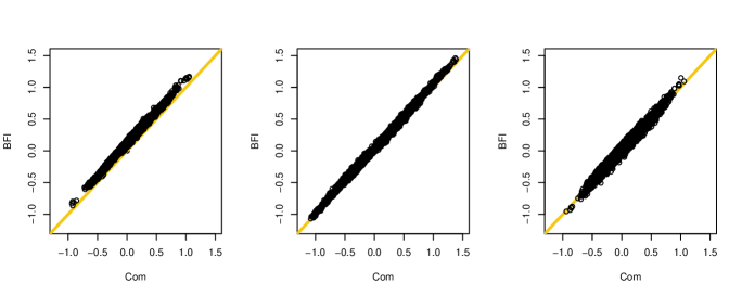
Figure 2: Outcome prediction based on the BFI strategy (vertical axis) versus those obtained after combining the training data sets (horizontal axis), for $\lambda=0.1$. Left: Heterogeneous populations. Predictions are based on the model that includes the covariates age, gender, experience, wardtype. Middle: Heterogeneous populations. Predictions are based on the model that includes the covariates hospital size, age, gender, experience, wardtype. Right: Homogeneous populations. Predictions are based on the model that includes the covariates age, gender, experience, wardtype. Perfect agreement corresponds to all points on the diagonal (yellow line).

4.3.2 Homogeneous populations

In the previous subsection we considered prediction accuracy of the BFI prediction model based on the data of nurses from the 25 hospitals. As mentioned before the nurses in the different hospitals may come from different populations. In this subsection we aim to study the performance of the BFI prediction model for homogeneous (nurse) populations. To be sure that the populations are homogeneous we randomize all nurses over the hospitals, keeping the sample sizes in the hospitals fixed. Now, the populations in the different hospitals can be seen as samples from the same population. Next, we follow the steps given in the previous subsection. This, including the randomization, is repeated 50 times. The variables we included in the model are age, gender, experience and wardtype. The scatter plot found for $\lambda=0.1$ is given in Figure 2, plot of the right. For other values of $\lambda$ the plots look similar. It can be seen that the agreement between the predictions is very strong. The scatter plot on the left in Figure 2 was obtained for the same model, but for the heterogeneous setting. In that case we saw some discrepancy between the predictions for the two models. Since this is not seen in the homogeneous setting and also not in the scatter plot for the models that take the hospital size into account, we conclude that discrepancy was due to the heterogeneity that was not taken into account in the first simulation.

5 Bayesian Federated Inference in R-Studio

We wrote the software package named BFI in Rstudio[11] for doing the BFI calculations as described in this paper. The R package and a short manual are available at github: https://hassanpazira.github.io/BFI. A detailed manual can also be found at https://github.com/hassanpazira/BFI/. In this section we explain how to do BFI analysis with the package: MAP-estimation (Subsection 5.1), BFI for homogeneous populations (Subsection 5.2), and for heterogeneous populations (Subsection 5.3).

5.1 MAP estimation

To fit a linear regression model and compute the MAP estimates of the parameters in the linear regression model, the command MAP.estimation can be used. To apply this command, the data has to be in a specific form and the inverse covariance matrix of the Gaussian prior distribution has to be chosen. The analysis below is for the combined data set Nurse. The estimates in the separate hospitals are obtained with the same command, but with the local data sets instead.

First a data frame M with the data of the model covariates is created:

   M <- data.frame(age=Nurses$age,gender=Nurses$gender,exp=Nurses$experien,
                        wardtype=Nurses$wardtype)

The prior distribution of the model parameters is assumed to be zero mean multivariate Gaussian. The dimension of its (inverse) covariance matrix depends on the number of parameters in the model; e.g. the number of regression parameters for a categorical variable equals the number of levels of the variable minus one. The command inv.prior.cov creates a diagonal inverse covariance matrix of the correct dimension:

   Lambda <- inv.prior.cov(M,lambda=c(0.01,0.01),family="gaussian")

The first argument is the data frame M, as defined before. Based on this data frame and the characteristics of the covariates (continuous or categorical) the number of parameters in the model is computed. The number of parameters also depends on the model that is fitted. A linear model (family="gaussian") has an extra parameter which is the standard deviation of the measurement error in the model. This parameter is absent for a logistic regression model (family="bionomial"). If the argument lambda=0.01 it means that all elements on the diagonal of $\Lambda$ equal 0.01. If two values are given, e.g. lambda=c(0.1,0.01), the first value (in this case 0.1) is on the diagonal of the inverse covariance matrix for all regression parameters, whereas the last value (0.01 here) is the value for the standard deviation of the measurement error. The latter is only valid for a linear regression model. Note that the values assigned to lambda should be positive always, as they equal 1 divided by a variance. Because $\Lambda$ is the inverse diagonal covariance matrix, values of $\lambda$ close to zero indicate a large variance of the prior distribution (the prior is not very informative) and a large value indicates a small variance (a very informative prior). Furthermore, because $\Lambda$ is a diagonal matrix, independence between the parameters is assumed. After setting the inverse covariance matrix, the MAP estimates can be computed with the function MAP.estimation. This command maximizes the log posterior density:

   fit <- MAP.estimation(Nurses$stress,X=M,family="gaussian",Lambda)
   summary(fit)

The arguments of this command are the outcome variable Nurses$stress, the covariate data in the dataframe M, the type of model that is fitted (family="gaussian") and the inverse covariance matrix Lambda. The MAP estimates are obtained by numerical maximization with the so-called Limited-memory Broyden-Fletcher-Goldfarb-Shanno algorithm with Bound Constraints (L-BFGS-B), [12]. As a starting point of the maximization 0 is taken by default, the mean of the prior distribution, but a different starting point can be chosen. The inference results are stored in the list fit. A summary of the MAP estimates is given with summary(fit). More detailed information on, e.g. the matrices $\widehat{{\bf A}}$ are printed by typing fit in R.

When applying the BFI approach, the statistical analyses as just described are performed in every (local) hospital and the results are sent to the central server. In practice this means that the output that is saved in fit is sent to the central server. There, the statistical results from the different hospitals are combined. This is explained in the next subsection.

5.2 Bayesian Federated Inference for homogeneous population

If we assume homogeneity across the hospitals, the BFI methodology as described in Section 2 can be applied. First the MAP estimates for the parameters in the linear regression models in the different hospitals are computed. Suppose that all hospitals have performed their analysis and sent their output of the command MAP.estimation to the central server. For ease of notation, we assume these outputs are stored in fit1, fit2, …, fit25. Now, from every output the relevant elements need to be selected and combined. In case of three hospitals the simplest way to do this is:

    thetahats <- list(fit1$theta_hat,fit2$theta_hat,fit3$theta_hat)
    Ahats     <- list(fit1$A_hat,fit2$A_hat,fit3$A_hat)
    priors    <- list(fit1$Lambda,fit2$Lambda,fit3$Lambda)

It is straightforward to extend this to 25 hospitals, but of course also more sophisticated methods are available in R. Once all the relevant elements are combined, the R code for computing the BFI estimators can be applied:

    priors <- append(priors,list(Lambda))
    fitbfi <- bfi(thetahats,Ahats,priors)
    summary(fitbfi)

Here Lambda is the inverse covariance matrix of the prior for the (fictive) combined data. The command bfi combines the estimates from the different hospitals into the BFI-estimates as explained in this paper. The command summary(fitbfi) gives the BFI estimates (and more information).

In our example we had access to all 25 data-sets. Because of that, the BFI analysis was performed with a for loop. The R code that was used is given below.

   thetahats <- Ahats <- priors <- list()
   for (i in 1:25)
     { Nursesi <- Nurses[Nurses$hospital==i,]
       Mi      <- data.frame(age=Nursesi$age,gender=Nursesi$gender,
                    experien=Nursesi$experien,wardtype=Nursesi$wardtype)
       Lambdai <- inv.prior.cov(Mi,lambda=0.01,family="gaussian")
       fiti    <- MAP.estimation(Nursesi$stress,X=Mi,family="gaussian",Lambdai)
       thetahats  <- append(thetahats,list(fiti$theta_hat))
       Ahats      <- append(Ahats,list(fiti$A_hat))
       priors     <- append(priors,list(fiti$Lambda))
     }
   Lambda <- Lambdai
   priors <- append(priors,list(Lambda))
   fitbfi <- bfi(thetahats,Ahats,priors)
   summary(fitbfi)

Within the for-loop the statistical analysis is performed in a single hospital. Because we have access to the data of all centers, the analysis results have been combined into lists for the estimates (thetahats), the $\widehat{A}$ matrices (Ahats) and the inverse covariance matrices (priors) directly. In practice this is not possible as all hospitals send the output fiti as described above. The outcome fitbfi is a list with the BFI estimates $\widehat{\mbox{\boldmath$\theta$}}$ and $\widehat{{\bf A}}$ and an overview of the results is given with the command summary(fitbfi).

5.3 BFI for heterogeneous populations

Different types of heterogeneity have been discussed in Section 3. Below we will explain how to do the analyses in Rstudio.

Heterogeneity of population characteristics
Heterogeneity across population characteristics in the centers implies that the value of the parameter $\mbox{\boldmath$\theta$}_{2}$ differs across centers. Because the bfi-command estimates the parameter $\mbox{\boldmath$\theta$}_{1}$ (and its curvature matrix $\widehat{A}_{1}$), and these estimates are not affected by $\mbox{\boldmath$\theta$}_{2}$, the R-code explained in the previous subsection can still be applied.

Heterogeneity across outcome means
Suppose the intercepts differ across hospitals. To take this variation into account we allow a hospital specific intercept in the regression model. Instead of one general intercept there are $L=25$ intercepts; an increase of $L-1$ parameters. The dimension of the inverse covariance matrix Lambda for the fictive combined data-set changes as well. For a diagonal matrix with 0.01 at the diagonal, this matrix can be obtained by

   Lambda <- inv.prior.cov(M,lambda=0.01,stratified=TRUE,strat_par=1,L=25)
   priors <- append(priors,list(Lambda))

These commands replace the two corresponding commands in Subsection 5.2. The argument L=25 had to be added to indicate the number of centers, and thus the number of location specific intercepts. This matrix should be appended to the list priors in stead. Like before, the MAP estimates of the regression parameters (and an estimate of $\widehat{\bf A}_{1}$) can be obtained with the command bfi, but it needs to be made explicit that the hospitals may have different intercepts:

   fitbfi <- bfi(thetahats,Ahats,priors,stratified=TRUE,strat_par=1)
   summary(fitbfi)

For this stratified analysis extra arguments have been added: stratified=TRUE and strat_par=1. The first argument indicates that the full model stratifies with respect to the different hospitals. The default value for stratified is FALSE. So, if the same model is assumed for all hospitals and for the model for all data, the argument can be left out. If strat_par=1 there is stratification with respect to the intercept and if strat_par=2 this is the case for the measurement error in a linear regression model. A summary of the results can be obtained by summary(fitbfi). This gives a list with estimates, starting with the hospital specific intercepts.

Heterogeneity due to center specific covariates
An example of a center specific covariate is hospital size. For all nurses in a hospital this covariate is constant and, as a consequence, the effect of hospital size on stress cannot be estimated within a hospital. However, the model for the (fictive) combined data could include this covariate if there is variation across the hospitals (Subsection 3.4). Here we explain how to do the analyses in Rstudio. In practice, every local hospital sends its size (small, medium, large) to the central server. There, a vector with all sizes is defined in Rstudio. Suppose this vector is named Hsize. After fitting the local models (like explained before), the estimated model for the (fictive) combined data can be obtained with:

   LambdaCom <- inv.prior.cov(Mi,lambda=0.01,stratified=TRUE,center_spec=Hsize,L=25)
   priors    <- append(priors,list(LambdaCom))
   fitbfi    <- bfi(thetahats,Ahats,priors,stratified=TRUE,center_spec=Hsize)
   summary(fitbfi)

Here, Hsize is a vector of length $L$ (the number of hospitals) with for every hospital its size category. The commands above return a list with categorical specific intercepts and the estimates of the regression coefficients of the remaining covariates.

For a continuous covariate the analysis is more complex. First the BFI estimates are computed allowing for different intercepts across the hospitals:

    fitbfi <- bfi(thetahats,Ahats,priors,stratified=T,strat_par=1)

Next, the estimated intercepts are plotted against the continuous hospital sizes. A least square line is fitted through these points:

    plot(Hsize,fitbfi$thetahats[1:25],xlab="hospital size",ylab="intercepts")
    lm(fitbfi$thetahats[1:25],Hsize)

The latter command gives estimates of the parameters $\nu_{0}$ and $\nu_{1}$ in the regression model (8).

6 Discussion

In this paper we have described the BFI strategy for generalized linear models for homogeneous and heterogeneous populations. The aim of the BFI methodology is to construct from the inference results obtained in multiple separate centers, what would have been found if the analysis had been performed on the combined data set. The key merit is that no individual data need to be transferred from the local centers to a central server. As a consequence, Data Transfer Agreement (DTA) for data sharing, can be simplified significantly. This may improve collaboration between researchers from different institutes and accelerate research.

In the paper, we first explain the methodology for homogeneous populations and next extend this to be able to deal with different types of heterogeneity across centers. The performance of the methodology is considered for multiple settings and is shown to be excellent for the estimates of the regression parameters and the predictions of the outcome. Furthermore, it is explained how to do the analyses in Rstudio with the software package BFI that we developed to make the methodology easily accessible for the user. The mathematical details are given in the appendix, but can be ignored if one’s interest is solely in the application of BFI.

In the BFI framework, statistical models are fitted in the separate centers based on local data only. So, in every center someone with sufficient knowledge of statistics and Rstudio needs to be available to do the analysis. Of course, the statistician who is concerned with combining the separate inference results can assist and can even provide code to be sure that the analyses in the separate centers are consistent.

The estimate $\widehat{\mbox{\boldmath$\theta$}}_{1}$ for the regression coefficients (and possibly other model parameters) does not depend on the estimates $\widehat{\mbox{\boldmath$\theta$}}_{2}$ and $\widehat{{\bf A}}_{2}$ (the population specific estimates). This means that heterogeneity across the population characteristics in the different centers do not affect the estimates that describe the association between the predictors and the outcome. So, even if the centers are located in different parts of the country or the world and serve populations with different characteristics, the strategy of combining the inference results for the regression models still holds under the assumption that the regression parameters are equal in the centers. And even if the latter is not expected for some covariates, the BFI strategy can take this into account.

The sets of variables available for fitting a regression model may differ across the centers. This happens, for instance, if some patients’ or individuals’ characteristics are measured and documented in most centers, but not in all. If a missing variable may be predictive for the outcome, a single or multiple regression method can be applied to impute the missing values[14]. Then, a regression model with this missing variable as an outcome and the original outcome variable and the remaining variables as covariates is fitted, by applying the BFI approach in the centers in which this “missing variable” has been measured. Next, this estimated regression model is used to predict the variable values in the center in which the variable was not measured. After a single or a multiple imputation, the BFI strategy as described before can be used.

The theory for the BFI approach has been developed for parametric models, including generalized linear models (GLMs). The Cox model for time-to-event data is a semi-parametric model. Developing the theory for this model and for even more complex models, will be the next step. The development of the theory will be accompanied by updates of the R package BFI.

The BFI methodology makes it possible to obtain the statistical power of the combined data set without actually combining the data. DTA’s can hence be simplified and collaboration between centers may increase.

Software
The R package BFI and a manual are available at github: https://hassanpazira.github.io/BFI . A detailed manual can also be found at https://github.com/hassanpazira/BFI/ .

Data availability statement
The trauma data are available in the R package BFI.

Funding
This research was supported by an unrestricted grant of Stichting Hanarth Fonds, The Netherlands.

Appendix: mathematical derivations of the BFI estimators

In this appendix the mathematical derivations of the BFI estimators are given for three settings:

1. Appendix A: Homogeneity across centers.

2. Appendix B: Heterogeneity across centers, center specific parameter, e.g. the intercept.

3. Appendix C: Heterogeneity across centers, center specific covariates.

Appendix A: Homogeneity across centers

In this appendix we derive expressions of the MAP estimators based on the data set ${\bf D}$ in terms of the local MAP estimators. In (2) and (2) we have seen that the log posterior densities for the (fictive) combined data set ${\bf D}$ and for the subset ${\bf D}_{\ell}$ equal

$$\log\big{\{}p(\mbox{\boldmath$\theta$}|{\bf D})\big{\}} =\;\log\big{\{}p(\theta_{1})\big{\}}\;+\;\log\big{\{}p(\theta_{2})\big{\}}\;+\;\sum_{\ell=1}^{L}\sum_{i=1}^{n_{\ell}}\log\big{\{}p(y_{\ell i}|{\bf x}_{\ell i},\mbox{\boldmath$\theta$}_{1})\big{\}}\;+\;\sum_{\ell=1}^{L}\sum_{i=1}^{n_{\ell}}\log\big{\{}p({\bf x}_{\ell i}|\mbox{\boldmath$\theta$}_{2})\big{\}}\;-\;\log\big{\{}p({\bf D})\big{\}}$$ (9)

$$\log\big{\{}p_{\ell}(\mbox{\boldmath$\theta$}|{\bf D}_{\ell})\big{\}} =\;\log\big{\{}p_{\ell}(\theta_{1})\big{\}}\;+\;\log\big{\{}p_{\ell}(\theta_{2})\big{\}}\;+\;\sum_{i=1}^{n_{\ell}}\log\big{\{}p(y_{\ell i}|{\bf x}_{\ell i},\mbox{\boldmath$\theta$}_{1})\big{\}}\;+\;\sum_{i=1}^{n_{\ell}}\log\big{\{}p({\bf x}_{\ell i}|\mbox{\boldmath$\theta$}_{2})\big{\}}\;-\;\log\big{\{}p_{\ell}({\bf D}_{\ell})\big{\}}.$$ (10)

By reordering the terms in equation (10), it follows that for every $\ell$

$$\sum_{i=1}^{n_{\ell}}\log\big{\{}p(y_{\ell i}|{\bf x}_{\ell i},\mbox{\boldmath$\theta$}_{1})\big{\}}\;+\;\sum_{i=1}^{n_{\ell}}\log\big{\{}p({\bf x}_{\ell i}|\mbox{\boldmath$\theta$}_{2})\big{\}}\;=\;\log\big{\{}p_{\ell}(\mbox{\boldmath$\theta$}|{\bf D}_{\ell})\big{\}}-\log\big{\{}p_{\ell}(\mbox{\boldmath$\theta$}_{1})\big{\}}\;-\;\log\big{\{}p_{\ell}(\mbox{\boldmath$\theta$}_{2})\big{\}}+\log\big{\{}p_{\ell}({\bf D}_{\ell})\big{\}}.$$

Next, summing over all centers yields

$$\sum_{\ell=1}^{L}\sum_{i=1}^{n_{\ell}}\log\big{\{}p(y_{\ell i}|{\bf x}_{\ell i},\mbox{\boldmath$\theta$}_{1})\big{\}}\;+\;\sum_{\ell=1}^{L}\sum_{i=1}^{n_{\ell}}\log\big{\{}p({\bf x}_{\ell i}|\mbox{\boldmath$\theta$}_{2})\big{\}}$$

$$~{}~{}~{}~{}~{}~{}~{}~{}=\;\sum_{\ell=1}^{L}\log\big{\{}p_{\ell}(\mbox{\boldmath$\theta$}|{\bf D}_{\ell})\big{\}}-\log\Big{\{}\prod_{\ell=1}^{L}p_{\ell}(\mbox{\boldmath$\theta$}_{1})\Big{\}}\;-\;\log\Big{\{}\prod_{\ell=1}^{L}p_{\ell}(\mbox{\boldmath$\theta$}_{2})\Big{\}}\;+\;\log\Big{\{}\prod_{\ell=1}^{L}p_{\ell}({\bf D}_{\ell})\Big{\}}.$$ (11)

By inserting the right hand side of (Appendix A: Homogeneity across centers) into the right hand side of (9) yields

$$\log\big{\{}p(\mbox{\boldmath$\theta$}|{\bf D})\big{\}}\;=\;\sum_{\ell=1}^{L}\log\big{\{}p_{\ell}(\mbox{\boldmath$\theta$}|{\bf D}_{\ell})\big{\}}+\log\Bigg{\{}\frac{p(\mbox{\boldmath$\theta$}_{1})}{\prod_{\ell=1}^{L}p_{\ell}(\mbox{\boldmath$\theta$}_{1})}\Bigg{\}}+\log\Bigg{\{}\frac{p(\mbox{\boldmath$\theta$}_{2})}{\prod_{\ell=1}^{L}p_{\ell}(\mbox{\boldmath$\theta$}_{2})}\Bigg{\}}-\log\Bigg{\{}\frac{\log p({\bf D})}{\prod_{\ell=1}^{L}\log p_{\ell}({\bf D}_{\ell})}\Bigg{\}}.$$ (12)

We expressed the log posterior densities of the combined data, $\log p(\mbox{\boldmath$\theta$}|{\bf D})$, in terms of the log posterior densities of the local data sets, $\log p_{\ell}(\mbox{\boldmath$\theta$}|{\bf D}_{\ell})$. However, the final aim is to express the MAP estimator $\widehat{\mbox{\boldmath$\theta$}}$ based on the (fictive) combined data set ${\bf D}$ in terms of the MAP estimators based on the local data sets ${\bf D}_{\ell}$. This will be done next. We approximate the log posterior densities for the combined data set ${\bf D}$ by a Taylor expansion up to the quadratic order in $\theta$ around the MAP estimator $\widehat{\mbox{\boldmath$\theta$}}$:

$$\log\big{\{}p\big{(}\mbox{\boldmath$\theta$}|{\bf D}\big{)}\big{\}}\;=\;\log\big{\{}p\big{(}\widehat{\mbox{\boldmath$\theta$}}|{\bf D}\big{)}\big{\}}-\tfrac{1}{2}\big{(}\mbox{\boldmath$\theta$}-\widehat{\mbox{\boldmath$\theta$}}\big{)}^{t}\widehat{{\bf A}}(\mbox{\boldmath$\theta$}-\widehat{\mbox{\boldmath$\theta$}}\big{)}+O_{p}\big{(}\|\mbox{\boldmath$\theta$}-\widehat{\mbox{\boldmath$\theta$}}\|^{3}\big{)},$$

with $\widehat{{\bf A}}$ equal to minus the second derivative of $\log\{p(\mbox{\boldmath$\theta$}|{\bf D})\}$ with respect to $\theta$, evaluated at $\widehat{\mbox{\boldmath$\theta$}}$. The linear term in the Taylor expansion is equal to zero and therefore missing in the expansion; the MAP estimator maximizes the log posterior density and the first derivative evaluated at $\widehat{\mbox{\boldmath$\theta$}}$ is therefore equal to zero. The last term in the Taylor expansion is equal to $O_{p}(\|\widehat{\mbox{\boldmath$\theta$}}-\mbox{\boldmath$\theta$}\|^{3})=\|\widehat{\mbox{\boldmath$\theta$}}-\mbox{\boldmath$\theta$}\|^{3}O_{p}(1)$, where $O_{p}(1)$ represents a term that is bounded in probability for the sample size going to infinity [13]. For $\theta$ in a small neighborhood of $\widehat{\mbox{\boldmath$\theta$}}$, the term $\|\widehat{\mbox{\boldmath$\theta$}}-\mbox{\boldmath$\theta$}\|^{3}$ will be close to zero (in probability), and the remainder term $O_{p}(\|\widehat{\mbox{\boldmath$\theta$}}-\mbox{\boldmath$\theta$}\|^{3})$ is small compared to the other terms in the Taylor expansion which are of an order of at most $\|\widehat{\mbox{\boldmath$\theta$}}-\mbox{\boldmath$\theta$}\|^{2}$. That means that

$$\log\big{\{}p\big{(}\mbox{\boldmath$\theta$}|{\bf D}\big{)}\big{\}}\;\approx\;\log\big{\{}p\big{(}\widehat{\mbox{\boldmath$\theta$}}|{\bf D}\big{)}\big{\}}-\tfrac{1}{2}\big{(}\mbox{\boldmath$\theta$}-\widehat{\mbox{\boldmath$\theta$}}\big{)}^{t}\widehat{{\bf A}}\big{(}\mbox{\boldmath$\theta$}-\widehat{\mbox{\boldmath$\theta$}}\big{)},$$

where the sign “$\approx$” means “is approximately equal to”. In the same way, the log posterior densities for the local subsets $\log\{p_{\ell}(\mbox{\boldmath$\theta$}|{\bf D}_{\ell})\}$ can be approximated around the MAP estimator $\widehat{\mbox{\boldmath$\theta$}}_{\ell}$:

$$\log\big{\{}p_{\ell}\big{(}\mbox{\boldmath$\theta$}|{\bf D}_{\ell}\big{)}\big{\}}\;\approx\;\log\big{\{}p_{\ell}\big{(}\widehat{\mbox{\boldmath$\theta$}}_{\ell}|{\bf D}_{\ell}\big{)}\big{\}}-\tfrac{1}{2}\big{(}\mbox{\boldmath$\theta$}-\widehat{\mbox{\boldmath$\theta$}}_{\ell}\big{)}^{t}\widehat{{\bf A}}_{\ell}\big{(}\mbox{\boldmath$\theta$}-\widehat{\mbox{\boldmath$\theta$}}_{\ell}\big{)},$$ (13)

with $\widehat{{\bf A}}_{\ell}$ equal to minus the second derivative of the log posterior density $\log\{p_{\ell}(\mbox{\boldmath$\theta$}|{\bf D}_{\ell})\}$ evaluated at $\widehat{\mbox{\boldmath$\theta$}}_{\ell}$. Since the log posterior densities in equations (9) and (10) are decomposed in terms that depend on either $\mbox{\boldmath$\theta$}_{1}$ or $\mbox{\boldmath$\theta$}_{2}$, but never on both, the matrices $\widehat{{\bf A}}$ and $\widehat{{\bf A}}_{\ell}$ are diagonal block matrices:

$$\widehat{{\bf A}}=\left(\!\begin{array}[]{cc}\widehat{{\bf A}}_{1}&{\bf 0}\\ {\bf 0}&\widehat{{\bf A}}_{2}\end{array}\!\right),~{}~{}~{}~{}~{}~{}~{}~{}\widehat{{\bf A}}_{\ell}=\left(\!\begin{array}[]{cc}\widehat{{\bf A}}_{1,\ell}&{\bf 0}\\ {\bf 0}&\widehat{{\bf A}}_{2,\ell}\end{array}\!\right),$$ (18)

with the blocks $\{\widehat{{\bf A}}_{1},\widehat{{\bf A}}_{1,\ell}\}$ and $\{\widehat{{\bf A}}_{2},\widehat{{\bf A}}_{2,\ell}\}$ equal to minus the second derivative matrices for $\mbox{\boldmath$\theta$}_{1}$ and $\mbox{\boldmath$\theta$}_{2}$, respectively, and the log posterior densities can be approximated by

$$\log\big{\{}p\big{(}\mbox{\boldmath$\theta$}|{\bf D}\big{)}\big{\}} \approx\;\log\big{\{}p\big{(}\widehat{\mbox{\boldmath$\theta$}}|{\bf D}\big{)}\big{\}}\;-\;\tfrac{1}{2}\big{(}\mbox{\boldmath$\theta$}_{1}-\widehat{\mbox{\boldmath$\theta$}}_{1}\big{)}^{t}\widehat{{\bf A}}_{1}\big{(}\mbox{\boldmath$\theta$}_{1}-\widehat{\mbox{\boldmath$\theta$}}_{1}\big{)}\;-\;\tfrac{1}{2}\big{(}\mbox{\boldmath$\theta$}_{2}-\widehat{\mbox{\boldmath$\theta$}}_{2}\big{)}^{t}\widehat{{\bf A}}_{2}\big{(}\mbox{\boldmath$\theta$}_{2}-\widehat{\mbox{\boldmath$\theta$}}_{2}\big{)}$$

$$\log\big{\{}p_{\ell}\big{(}\mbox{\boldmath$\theta$}|{\bf D}_{\ell}\big{)}\big{\}} \approx\;\log\big{\{}p_{\ell}\big{(}\widehat{\mbox{\boldmath$\theta$}}_{\ell}|{\bf D}_{\ell}\big{)}\big{\}}\;-\;\tfrac{1}{2}\big{(}\mbox{\boldmath$\theta$}_{1}-\widehat{\mbox{\boldmath$\theta$}}_{1,\ell}\big{)}^{t}\widehat{{\bf A}}_{1,\ell}\big{(}\mbox{\boldmath$\theta$}_{1}-\widehat{\mbox{\boldmath$\theta$}}_{1,\ell}\big{)}\;-\;\tfrac{1}{2}\big{(}\mbox{\boldmath$\theta$}_{2}-\widehat{\mbox{\boldmath$\theta$}}_{2,\ell}\big{)}^{t}\widehat{{\bf A}}_{2,\ell}\big{(}\mbox{\boldmath$\theta$}_{2}-\widehat{\mbox{\boldmath$\theta$}}_{2,\ell}\big{)}.$$

By substituting these approximations for $\log\{p(\mbox{\boldmath$\theta$}|{\bf D})\}$ and $\log\{p_{\ell}(\mbox{\boldmath$\theta$}|{\bf D}_{\ell})\},\ell=1,\ldots,L$, into the relation (12), we obtain:

$$\big{(}\mbox{\boldmath$\theta$}_{1}-\widehat{\mbox{\boldmath$\theta$}}_{1}\big{)}^{t}\widehat{{\bf A}}_{1}\big{(}\mbox{\boldmath$\theta$}_{1}-\widehat{\mbox{\boldmath$\theta$}}_{1}\big{)}\;+\;\big{(}\mbox{\boldmath$\theta$}_{2}-\widehat{\mbox{\boldmath$\theta$}}_{2}\big{)}^{t}\widehat{{\bf A}}_{2}\big{(}\mbox{\boldmath$\theta$}_{2}-\widehat{\mbox{\boldmath$\theta$}}_{2}\big{)}$$ (19)

$$\approx\;\sum_{\ell=1}^{L}\big{(}\mbox{\boldmath$\theta$}_{1}-\widehat{\mbox{\boldmath$\theta$}}_{1,\ell}\big{)}^{t}\widehat{{\bf A}}_{1,\ell}\big{(}\mbox{\boldmath$\theta$}_{1}-\widehat{\mbox{\boldmath$\theta$}}_{1,\ell}\big{)}\;+\;\sum_{\ell=1}^{L}\big{(}\mbox{\boldmath$\theta$}_{2}-\widehat{\mbox{\boldmath$\theta$}}_{2,\ell}\big{)}^{t}\widehat{{\bf A}}_{2,\ell}\big{(}\mbox{\boldmath$\theta$}_{2}-\widehat{\mbox{\boldmath$\theta$}}_{2,\ell}\big{)}\;-\;2\log\Bigg{\{}\frac{p(\mbox{\boldmath$\theta$}_{1})}{\prod_{\ell=1}^{L}p_{\ell}(\mbox{\boldmath$\theta$}_{1})}\Bigg{\}}\;-\;2\log\Bigg{\{}\frac{p(\mbox{\boldmath$\theta$}_{2})}{\prod_{\ell=1}^{L}p_{\ell}(\mbox{\boldmath$\theta$}_{2})}\Bigg{\}}\;+\;B.$$

where $B$ is a term that depends on the data, but is not a function of $\mbox{\boldmath$\theta$}=(\mbox{\boldmath$\theta$}_{1},\mbox{\boldmath$\theta$}_{2})$. Seen as a function of $\mbox{\boldmath$\theta$}_{1}$ and $\mbox{\boldmath$\theta$}_{2}$, this yields

$$\big{(}\mbox{\boldmath$\theta$}_{1}-\widehat{\mbox{\boldmath$\theta$}}_{1}\big{)}^{t}\widehat{{\bf A}}_{1}\big{(}\mbox{\boldmath$\theta$}_{1}-\widehat{\mbox{\boldmath$\theta$}}_{1}\big{)} \approx\;\sum_{\ell=1}^{L}\big{(}\mbox{\boldmath$\theta$}_{1}-\widehat{\mbox{\boldmath$\theta$}}_{1,\ell}\big{)}^{t}\widehat{{\bf A}}_{1,\ell}\big{(}\mbox{\boldmath$\theta$}_{1}-\widehat{\mbox{\boldmath$\theta$}}_{1,\ell}\big{)}\;-\;2\log\Bigg{\{}\frac{p(\mbox{\boldmath$\theta$}_{1})}{\prod_{\ell=1}^{L}p_{\ell}(\mbox{\boldmath$\theta$}_{1})}\Bigg{\}}\;+\;B_{1}.$$ (20)

$$\big{(}\mbox{\boldmath$\theta$}_{2}-\widehat{\mbox{\boldmath$\theta$}}_{2}\big{)}^{t}\widehat{{\bf A}}_{2}\big{(}\mbox{\boldmath$\theta$}_{2}-\widehat{\mbox{\boldmath$\theta$}}_{2}\big{)} \approx\;\sum_{\ell=1}^{L}\big{(}\mbox{\boldmath$\theta$}_{2}-\widehat{\mbox{\boldmath$\theta$}}_{2,\ell}\big{)}^{t}\widehat{{\bf A}}_{2,\ell}\big{(}\mbox{\boldmath$\theta$}_{2}-\widehat{\mbox{\boldmath$\theta$}}_{2,\ell}\big{)}\;-\;2\log\Bigg{\{}\frac{p(\mbox{\boldmath$\theta$}_{2})}{\prod_{\ell=1}^{L}p_{\ell}(\mbox{\boldmath$\theta$}_{2})}\Bigg{\}}\;+\;B_{2}.$$ (21)

for $B_{1}$ and $B_{2}$ terms that depend on the data, but are no functions of $\mbox{\boldmath$\theta$}_{1}$ and $\mbox{\boldmath$\theta$}_{2}$. Now choose the prior densities $\mbox{\boldmath$\theta$}_{1}\rightarrow p(\mbox{\boldmath$\theta$}_{1})$ and $\mbox{\boldmath$\theta$}_{2}\rightarrow p(\mbox{\boldmath$\theta$}_{2})$ in the combined data set and $\mbox{\boldmath$\theta$}_{1}\rightarrow p_{\ell}(\mbox{\boldmath$\theta$}_{1})$ and $\mbox{\boldmath$\theta$}_{2}\rightarrow p_{\ell}(\mbox{\boldmath$\theta$}_{2})$ in center $\ell$ to be Gaussian with mean zero and inverse covariance matrices $\mbox{\boldmath$\Lambda$}_{1}$ and $\mbox{\boldmath$\Lambda$}_{2}$ in the combined data set, and $\mbox{\boldmath$\Lambda$}_{1,\ell}$ and $\mbox{\boldmath$\Lambda$}_{2,\ell}$ in center $\ell$: e.g. $p(\mbox{\boldmath$\theta$}_{1})=(\det\mbox{\boldmath$\Lambda$}_{1}/(2\pi)^{d})^{1/2}\exp(-\tfrac{1}{2}\mbox{\boldmath$\theta$}_{1}^{t}\mbox{\boldmath$\Lambda$}_{1}\mbox{\boldmath$\theta$}_{1})$. Inserting the expressions of the densities into (20) and (21) yield

$$\big{(}\mbox{\boldmath$\theta$}_{1}-\widehat{\mbox{\boldmath$\theta$}}_{1}\big{)}^{t}\widehat{{\bf A}}_{1}\big{(}\mbox{\boldmath$\theta$}_{1}-\widehat{\mbox{\boldmath$\theta$}}_{1}\big{)} \approx\;\sum_{\ell=1}^{L}\big{(}\mbox{\boldmath$\theta$}_{1}-\widehat{\mbox{\boldmath$\theta$}}_{1,\ell}\big{)}^{t}\widehat{{\bf A}}_{1,\ell}\big{(}\mbox{\boldmath$\theta$}_{1}-\widehat{\mbox{\boldmath$\theta$}}_{1,\ell}\big{)}\;+\;\mbox{\boldmath$\theta$}_{1}^{t}\Big{(}\Lambda_{1}-\sum_{\ell=1}^{L}\mbox{\boldmath$\Lambda$}_{1,\ell}\Big{)}\mbox{\boldmath$\theta$}_{1}\;+\;B_{1}^{\prime},$$ (22)

$$\big{(}\mbox{\boldmath$\theta$}_{2}-\widehat{\mbox{\boldmath$\theta$}}_{2}\big{)}^{t}\widehat{{\bf A}}_{2}\big{(}\mbox{\boldmath$\theta$}_{2}-\widehat{\mbox{\boldmath$\theta$}}_{2}\big{)} \approx\;\sum_{\ell=1}^{L}\big{(}\mbox{\boldmath$\theta$}_{2}-\widehat{\mbox{\boldmath$\theta$}}_{2,\ell}\big{)}^{t}\widehat{{\bf A}}_{2,\ell}\big{(}\mbox{\boldmath$\theta$}_{2}-\widehat{\mbox{\boldmath$\theta$}}_{2,\ell}\big{)}\;+\;\mbox{\boldmath$\theta$}_{2}^{t}\Big{(}\Lambda_{2}-\sum_{\ell=1}^{L}\mbox{\boldmath$\Lambda$}_{2,\ell}\Big{)}\mbox{\boldmath$\theta$}_{2}\;+\;B_{2}^{\prime},$$ (23)

for $B_{1}^{\prime}$ and $B_{2}^{\prime}$ terms that depend on the data, but not of $\mbox{\boldmath$\theta$}_{1}$ and $\mbox{\boldmath$\theta$}_{2}$. The left and right hand side of the approximations in (22) and (23) are quadratic functions of $\mbox{\boldmath$\theta$}_{1}$ and $\mbox{\boldmath$\theta$}_{2}$, respectively. These equalities only hold if the coefficients of the linear and the quadratic terms are the same on the left and right hand side. By solving the approximations with respect to $\widehat{\mbox{\boldmath$\theta$}}_{1},\widehat{\mbox{\boldmath$\theta$}}_{2},\widehat{{\bf A}}_{1}$ and $\widehat{{\bf A}}_{2}$, the following expressions are found

$$\widehat{{\bf A}}_{1}\approx\sum_{\ell=1}^{L}\widehat{{\bf A}}_{1,\ell}+\mbox{\boldmath$\Lambda$}_{1}-\sum_{\ell=1}^{L}\mbox{\boldmath$\Lambda$}_{1,\ell},~{}~{}~{}~{}~{}~{}~{}~{}~{}~{}~{}~{}~{}\widehat{\mbox{\boldmath$\theta$}}_{1}\approx\big{(}\widehat{{\bf A}}_{1}\big{)}^{-1}\sum_{\ell=1}^{L}\widehat{{\bf A}}_{1,\ell}\widehat{\mbox{\boldmath$\theta$}}_{1,\ell},$$

$$\widehat{{\bf A}}_{2}\approx\sum_{\ell=1}^{L}\widehat{{\bf A}}_{2,\ell}+\mbox{\boldmath$\Lambda$}_{2}-\sum_{\ell=1}^{L}\mbox{\boldmath$\Lambda$}_{2,\ell},~{}~{}~{}~{}~{}~{}~{}~{}~{}~{}~{}~{}~{}\widehat{\mbox{\boldmath$\theta$}}_{2}\approx\big{(}\widehat{{\bf A}}_{2}\big{)}^{-1}\sum_{\ell=1}^{L}\widehat{{\bf A}}_{2,\ell}\widehat{\mbox{\boldmath$\theta$}}_{2,\ell}.$$

Appendix B: Heterogeneity across centers, center-specific parameter

In this appendix we assume that the vector of regression parameters can be subdivided into two parts. One part is equal across the centers and the other part may vary. A special case is the situation in which the intercepts vary. In this appendix the MAP estimators based on the full data set ${\bf D}$ are expressed in terms of the local MAP estimators.

Suppose that the vector $\theta$ can be decomposed as $\mbox{\boldmath$\theta$}=(\mbox{\boldmath$\theta$}_{1},\mbox{\boldmath$\theta$}_{2})=(\mbox{\boldmath$\theta$}_{1a},\mbox{\boldmath$\theta$}_{1b},\mbox{\boldmath$\theta$}_{2})$, where, as before, $\mbox{\boldmath$\theta$}_{2}$ is the vector of parameters that specifies the distribution of the covariates. The parameter $\mbox{\boldmath$\theta$}_{1}=(\mbox{\boldmath$\theta$}_{1a},\mbox{\boldmath$\theta$}_{1b})$ is decomposed so that $\mbox{\boldmath$\theta$}_{1a}$ is the vector of (regression) parameters that is assumed to be equal in the different sub-populations, and $\mbox{\boldmath$\theta$}_{1b}$ is the vector of (regression) parameters that may vary across the sub-populations. In this appendix we consider the situation that every center has its own specific vector: $\mbox{\boldmath$\theta$}_{1b,1},\ldots,\mbox{\boldmath$\theta$}_{1b,L}$ for the $L$ centers. The vector of parameters in the combined data set is equal to $\mbox{\boldmath$\theta$}=(\mbox{\boldmath$\theta$}_{1a},\mbox{\boldmath$\theta$}_{1b,1},\ldots,\mbox{\boldmath$\theta$}_{1b,L},\mbox{\boldmath$\theta$}_{2})$, where $\mbox{\boldmath$\theta$}_{1b,\ell}$ is the parameter vector in center $\ell$. If only the intercepts vary across the centers $\mbox{\boldmath$\theta$}_{1b,\ell}$ is one-dimensional, but for now we allow $\mbox{\boldmath$\theta$}_{1b,\ell}$ to be a vector.

For simplicity of notation we assume that $\mbox{\boldmath$\theta$}_{1a},\mbox{\boldmath$\theta$}_{1b}$ and $\mbox{\boldmath$\theta$}_{2}$ are independent: $p(\mbox{\boldmath$\theta$})=p(\mbox{\boldmath$\theta$}_{1a})\prod_{\ell=1}^{L}p(\mbox{\boldmath$\theta$}_{1b,\ell})p(\mbox{\boldmath$\theta$}_{2})$ for the combined data set, and in center $\ell$: $p_{\ell}(\mbox{\boldmath$\theta$}_{1a},\mbox{\boldmath$\theta$}_{1b,\ell},\mbox{\boldmath$\theta$}_{2})=p_{\ell}(\mbox{\boldmath$\theta$}_{1a})p_{\ell}(\mbox{\boldmath$\theta$}_{1b,\ell})p_{\ell}(\mbox{\boldmath$\theta$}_{2})$. The log posterior densities are given by

$$\log\big{\{}p(\mbox{\boldmath$\theta$}|{\bf D})\big{\}}$$

$$=\;\log\big{\{}p(\mbox{\boldmath$\theta$}_{1a})\big{\}}+\sum_{\ell=1}^{L}\log\big{\{}p(\mbox{\boldmath$\theta$}_{1b,\ell})\big{\}}+\log\big{\{}p(\mbox{\boldmath$\theta$}_{2})\big{\}}+\sum_{\ell=1}^{L}\sum_{i=1}^{n_{\ell}}\log\big{\{}p(y_{\ell i}|\mbox{\boldmath$\theta$}_{1a},\mbox{\boldmath$\theta$}_{1b,\ell},{\bf x}_{\ell i})\big{\}}+\sum_{\ell=1}^{L}\sum_{i=1}^{n_{\ell}}\log\big{\{}p({\bf x}_{\ell i}|\mbox{\boldmath$\theta$}_{2})\big{\}}-\log\big{\{}p({\bf D})\big{\}},$$

and

$$\log\big{\{}p_{\ell}(\mbox{\boldmath$\theta$}_{1a},\mbox{\boldmath$\theta$}_{1b,\ell},\mbox{\boldmath$\theta$}_{2}|{\bf D}_{\ell})\big{\}}$$

$$=\;\log\big{\{}p_{\ell}(\mbox{\boldmath$\theta$}_{1a})\big{\}}+\log\big{\{}p_{\ell}(\mbox{\boldmath$\theta$}_{1b,\ell})\big{\}}+\log\big{\{}p_{\ell}(\mbox{\boldmath$\theta$}_{2})\big{\}}+\sum_{i=1}^{n_{\ell}}\log\big{\{}p(y_{\ell i}|\mbox{\boldmath$\theta$}_{1a},\mbox{\boldmath$\theta$}_{1b,\ell},{\bf x}_{\ell i})\big{\}}+\sum_{i=1}^{n_{\ell}}\log\big{\{}p({\bf x}_{\ell i}|\mbox{\boldmath$\theta$}_{2})\big{\}}-\log\big{\{}p_{\ell}({\bf D}_{\ell})\big{\}}.$$

Previously, and in the formulas above, we see that the log posterior density is decomposed into terms that depend on $\mbox{\boldmath$\theta$}_{1}$ or $\mbox{\boldmath$\theta$}_{2}$, but never on both. That means that, as we have seen before, the BFI estimator for $\mbox{\boldmath$\theta$}_{1}$ is not affected by the estimator $\mbox{\boldmath$\theta$}_{2}$ and vice versa. Therefore, in this setting, the BFI estimator $\widehat{\mbox{\boldmath$\theta$}}_{2}$ can be expressed in terms of the local MAP estimators $\widehat{\mbox{\boldmath$\theta$}}_{2,\ell}$ and $\widehat{A}_{2,\ell}$ as in (4). In the remainder of the derivation we focus on $\mbox{\boldmath$\theta$}_{1}$ only and leave out the terms with $\mbox{\boldmath$\theta$}_{2}$ from the expressions.

As before, the log posterior density in the full data set can be written in terms of the local log posterior densities:

$$\log\big{\{}p(\mbox{\boldmath$\theta$}|{\bf D})\big{\}}\;=\;\sum_{\ell=1}^{L}\log\big{\{}p_{\ell}(\mbox{\boldmath$\theta$}_{1a},\mbox{\boldmath$\theta$}_{1b,\ell}|{\bf D}_{\ell})\big{\}}+\log\Bigg{\{}\frac{p(\mbox{\boldmath$\theta$}_{1a})}{\prod_{\ell=1}^{L}p_{\ell}(\mbox{\boldmath$\theta$}_{1a})}\Bigg{\}}\;+\;\log\Bigg{\{}\frac{\prod_{\ell=1}^{L}p(\mbox{\boldmath$\theta$}_{1b,\ell})}{\prod_{\ell=1}^{L}p_{\ell}(\mbox{\boldmath$\theta$}_{1b,\ell})}\Bigg{\}}+B$$ (24)

with $B$ a term that depends on the data and on $\mbox{\boldmath$\theta$}_{2}$, but is not a function of $\mbox{\boldmath$\theta$}_{1}$.

Let $\widetilde{\mbox{\boldmath$\theta$}}_{1b,\ell}$ be the MAP estimator of $\mbox{\boldmath$\theta$}_{1b,\ell}$ based on the full data set ${\bf D}$. Moreover, let $\widetilde{{\bf A}}_{1b,\ell}$ be equal to minus the second derivatives of $\log\{p(\mbox{\boldmath$\theta$}|{\bf D})\}$ with respect to the components of $\mbox{\boldmath$\theta$}_{1b,\ell}$, and let $\widetilde{{\bf A}}_{1ab,\ell}$ be minus the second derivative with respect to both $\mbox{\boldmath$\theta$}_{1a}$ and $\mbox{\boldmath$\theta$}_{1b,\ell}$ both evaluated at $(\widehat{\mbox{\boldmath$\theta$}}_{1a},\widetilde{\mbox{\boldmath$\theta$}}_{1b,\ell})$. The corresponding estimators based on the local data set ${\bf D}_{\ell}$ are denoted with a “hat” in stead of a “tilde”: $\widehat{\mbox{\boldmath$\theta$}}_{1b,\ell}$, $\widehat{{\bf A}}_{1b,\ell}$ and $\widehat{{\bf A}}_{1ab,\ell}$.

The Taylor expansions of $\log\{p(\mbox{\boldmath$\theta$}|{\bf D})\}$ and $\log\{p_{\ell}(\mbox{\boldmath$\theta$}|{\bf D}_{\ell})\}$, around $\widehat{\mbox{\boldmath$\theta$}}_{1}$ and $\widehat{\mbox{\boldmath$\theta$}}_{\ell,1}$ respectively, up to the quadratic term are

$$\log\big{\{}p\big{(}\mbox{\boldmath$\theta$}|{\bf D}\big{)}\big{\}} \approx\;\log\big{\{}p\big{(}\widehat{\mbox{\boldmath$\theta$}}|{\bf D}\big{)}\big{\}}-\tfrac{1}{2}\big{(}\mbox{\boldmath$\theta$}_{1a}-\widehat{\mbox{\boldmath$\theta$}}_{1a}\big{)}^{t}\widehat{{\bf A}}_{1a}\big{(}\mbox{\boldmath$\theta$}_{1a}-\widehat{\mbox{\boldmath$\theta$}}_{1a}\big{)}$$

$$\qquad-\;\tfrac{1}{2}\sum_{\ell=1}^{L}\big{(}\mbox{\boldmath$\theta$}_{1b,\ell}-\widetilde{\mbox{\boldmath$\theta$}}_{1b,\ell}\big{)}^{t}\widetilde{{\bf A}}_{1b,\ell}\big{(}\mbox{\boldmath$\theta$}_{1b,\ell}-\widetilde{\mbox{\boldmath$\theta$}}_{1b,\ell}\big{)}-\big{(}\mbox{\boldmath$\theta$}_{1a}-\widehat{\mbox{\boldmath$\theta$}}_{1a}\big{)}^{t}\sum_{\ell=1}^{L}\widetilde{{\bf A}}_{1ab,\ell}\big{(}\mbox{\boldmath$\theta$}_{1b,\ell}-\widetilde{\mbox{\boldmath$\theta$}}_{1b,\ell}\big{)},$$

$$\log\big{\{}p_{\ell}\big{(}\mbox{\boldmath$\theta$}|{\bf D}_{\ell}\big{)}\big{\}} \approx\;\log\big{\{}p_{\ell}\big{(}\widehat{\mbox{\boldmath$\theta$}}_{\ell}|{\bf D}_{\ell}\big{)}\big{\}}-\tfrac{1}{2}\big{(}\mbox{\boldmath$\theta$}_{1a}-\widehat{\mbox{\boldmath$\theta$}}_{1a,\ell}\big{)}^{t}\widehat{{\bf A}}_{1a,\ell}\big{(}\mbox{\boldmath$\theta$}_{1a}-\widehat{\mbox{\boldmath$\theta$}}_{1a,\ell}\big{)}$$

$$\qquad-\;\tfrac{1}{2}\big{(}\mbox{\boldmath$\theta$}_{1b,\ell}-\widehat{\mbox{\boldmath$\theta$}}_{1b,\ell}\big{)}^{t}\widehat{{\bf A}}_{1b,\ell}\big{(}\mbox{\boldmath$\theta$}_{1b,\ell}-\widehat{\mbox{\boldmath$\theta$}}_{1b,\ell}\big{)}-\big{(}\mbox{\boldmath$\theta$}_{1a}-\widehat{\mbox{\boldmath$\theta$}}_{1a,\ell}\big{)}^{t}\widehat{{\bf A}}_{1ab,\ell}\big{(}\mbox{\boldmath$\theta$}_{1b,\ell}-\widehat{\mbox{\boldmath$\theta$}}_{1b,\ell}\big{)}.$$

Next, we insert the Taylor expressions into (24). For the combined data ${\bf D}$ we assume a Gaussian prior with mean zero and inverse covariance matrix $\mbox{\boldmath$\Lambda$}_{1a}$ for $\mbox{\boldmath$\theta$}_{1a}$, and a zero mean Gaussian prior with inverse covariance matrix $\mbox{\boldmath$\Lambda$}_{1b\ell}$ for $\mbox{\boldmath$\theta$}_{1b,\ell},\ell=1,\ldots,L$. For center $\ell$, also zero mean Gaussian priors are chosen, but with inverse covariance matrices $\mbox{\boldmath$\Lambda$}_{1a,\ell}$ and $\mbox{\boldmath$\Lambda$}_{1b,\ell}$. The dimension of $\mbox{\boldmath$\Lambda$}_{1b\ell}$ and $\mbox{\boldmath$\Lambda$}_{1b,\ell}$ depends on the number of parameters that may vary across the centers. In case only the intercepts vary, the matrices are scalars. After inserting the expressions of these densities in (24) as well, we obtain

$$\big{(}\mbox{\boldmath$\theta$}_{1a}-\widehat{\mbox{\boldmath$\theta$}}_{1a}\big{)}^{t}\widehat{{\bf A}}_{1a}\big{(}\mbox{\boldmath$\theta$}_{1a}-\widehat{\mbox{\boldmath$\theta$}}_{1a}\big{)}+\sum_{\ell=1}^{L}\big{(}\mbox{\boldmath$\theta$}_{1b,\ell}-\widetilde{\mbox{\boldmath$\theta$}}_{1b,\ell}\big{)}^{t}\widetilde{{\bf A}}_{1b,\ell}\big{(}\mbox{\boldmath$\theta$}_{1b,\ell}-\widetilde{\mbox{\boldmath$\theta$}}_{1b,\ell}\big{)}+\;2\big{(}\mbox{\boldmath$\theta$}_{1a}-\widehat{\mbox{\boldmath$\theta$}}_{1a}\big{)}^{t}\sum_{\ell=1}^{L}\widetilde{{\bf A}}_{1ab,\ell}\big{(}\mbox{\boldmath$\theta$}_{1b,\ell}-\widetilde{\mbox{\boldmath$\theta$}}_{1b,\ell}\big{)}$$

$$\hskip 14.22636pt\approx\;\sum_{\ell=1}^{L}\big{(}\mbox{\boldmath$\theta$}_{1a}-\widehat{\mbox{\boldmath$\theta$}}_{1a,\ell}\big{)}^{t}\widehat{{\bf A}}_{1a,\ell}\big{(}\mbox{\boldmath$\theta$}_{1a}-\widehat{\mbox{\boldmath$\theta$}}_{1a,\ell}\big{)}+\mbox{\boldmath$\theta$}_{1a}^{t}\Big{(}\mbox{\boldmath$\Lambda$}_{1a}-\sum_{\ell=1}^{L}\mbox{\boldmath$\Lambda$}_{1a,\ell}\Big{)}\mbox{\boldmath$\theta$}_{1a}\;+\;\sum_{\ell=1}^{L}\big{(}\mbox{\boldmath$\theta$}_{1b,\ell}-\widehat{\mbox{\boldmath$\theta$}}_{1b,\ell}\big{)}^{t}\widehat{{\bf A}}_{1b,\ell}\big{(}\mbox{\boldmath$\theta$}_{1b,\ell}-\widehat{\mbox{\boldmath$\theta$}}_{1b,\ell}\big{)}$$ (25)

$$\hskip 28.45274pt\;+\;\sum_{\ell=1}^{L}\mbox{\boldmath$\theta$}_{1b,\ell}^{t}\big{(}\mbox{\boldmath$\Lambda$}_{1b\ell}-\mbox{\boldmath$\Lambda$}_{1b,\ell}\big{)}\mbox{\boldmath$\theta$}_{1b,\ell}\;+\;2\sum_{\ell=1}^{L}\big{(}\mbox{\boldmath$\theta$}_{1a}-\widehat{\mbox{\boldmath$\theta$}}_{1a,\ell}\big{)}^{t}\widehat{{\bf A}}_{1ab,\ell}\big{(}\mbox{\boldmath$\theta$}_{1b,\ell}-\widehat{\mbox{\boldmath$\theta$}}_{1b,\ell}\big{)}+B^{\prime}$$

with $B^{\prime}$ representing a term that does not depend on $\mbox{\boldmath$\theta$}_{1}$. The left and right hand side of the equation are quadratic functions of $\mbox{\boldmath$\theta$}_{1a}$ and $\mbox{\boldmath$\theta$}_{1b}$. Since the equation must hold for all values of $\mbox{\boldmath$\theta$}_{1}=(\mbox{\boldmath$\theta$}_{1a},\mbox{\boldmath$\theta$}_{1b})$ in a neighborhoud of the MAP estimator $\widehat{\mbox{\boldmath$\theta$}}_{1}$, the coefficients on either side of the specific linear terms must equal, as well as those of the quadratic terms. For the quadratic terms, this gives:

$$\widehat{{\bf A}}_{1a}\approx\sum_{\ell=1}^{L}\widehat{{\bf A}}_{1a,\ell}+\mbox{\boldmath$\Lambda$}_{1a}-\sum_{\ell=1}^{L}\mbox{\boldmath$\Lambda$}_{1a,\ell},~{}~{}~{}~{}~{}~{}~{}\widetilde{{\bf A}}_{1b,\ell}\approx\widehat{{\bf A}}_{1b,\ell}+\mbox{\boldmath$\Lambda$}_{1b\ell}-\mbox{\boldmath$\Lambda$}_{1b,\ell},~{}~{}~{}~{}~{}~{}~{}\widetilde{{\bf A}}_{1ab,\ell}\approx\widehat{{\bf A}}_{1ab,\ell},$$ (26)

and for the linear terms

$$\widehat{{\bf A}}_{1a}\widehat{\mbox{\boldmath$\theta$}}_{1a}+\sum_{\ell=1}^{L}\widetilde{{\bf A}}_{1ab,\ell}\widetilde{\mbox{\boldmath$\theta$}}_{1b,\ell} \approx\;\sum_{\ell=1}^{L}\widehat{{\bf A}}_{1a,\ell}\widehat{\mbox{\boldmath$\theta$}}_{1a,\ell}+\sum_{\ell=1}^{L}\widehat{{\bf A}}_{1ab,\ell}\widehat{\mbox{\boldmath$\theta$}}_{1b,\ell},$$

$$\widetilde{{\bf A}}_{1b,\ell}\widetilde{\mbox{\boldmath$\theta$}}_{1b,\ell}+(\widetilde{{\bf A}}_{1ab,\ell})^{t}\widehat{\mbox{\boldmath$\theta$}}_{1a} \approx\;\widehat{{\bf A}}_{1b,\ell}\widehat{\mbox{\boldmath$\theta$}}_{1b,\ell}+(\widehat{{\bf A}}_{1ab,\ell})^{t}\widehat{\mbox{\boldmath$\theta$}}_{1a,\ell}.$$

Solving these equations yield expressions for the estimators $\widehat{\mbox{\boldmath$\theta$}}_{1a}$ and $\widetilde{\mbox{\boldmath$\theta$}}_{1b,\ell}$:

$$\widehat{\mbox{\boldmath$\theta$}}_{1a}\approx\Big{(}\widehat{{\bf A}}_{1a}-\sum_{\ell=1}^{L}\widehat{{\bf A}}_{1ab,\ell}(\widetilde{{\bf A}}_{1b,\ell})^{-1}(\widetilde{{\bf A}}_{1ab,\ell})^{t}\Big{)}^{\!-1}\sum_{\ell=1}^{L}\Big{[}\Big{(}\widehat{{\bf A}}_{1a,\ell}-\widehat{{\bf A}}_{1ab,\ell}(\widetilde{{\bf A}}_{1b,\ell})^{-1}(\widehat{{\bf A}}_{1ab,\ell})^{t}\Big{)}\widehat{\mbox{\boldmath$\theta$}}_{1a,\ell}+\widehat{{\bf A}}_{1ab,\ell}\Big{(}{\bf 1}-(\widetilde{{\bf A}}_{1b,\ell})^{-1}\widehat{{\bf A}}_{1b,\ell}\Big{)}\widehat{\mbox{\boldmath$\theta$}}_{1b,\ell}\Big{]}~{}~{}$$

with ${\bf 1}$ the unit matrix and the matrices $\widehat{{\bf A}}_{a}$ and $\widetilde{{\bf A}}_{b,\ell}$ as given in (26). The estimators $\widetilde{\mbox{\boldmath$\theta$}}_{1b,\ell}$ are given by

$$\widetilde{\mbox{\boldmath$\theta$}}_{1b,\ell}\approx\big{(}\widetilde{{\bf A}}_{1b,\ell}\big{)}^{-1}\Big{[}\widehat{{\bf A}}_{1b,\ell}\widehat{\mbox{\boldmath$\theta$}}_{1b,\ell}+\big{(}\widehat{{\bf A}}_{1ab,\ell}\big{)}^{t}\big{(}\widehat{\mbox{\boldmath$\theta$}}_{1a,\ell}-\widehat{\mbox{\boldmath$\theta$}}_{1a}\big{)}\Big{]}.$$

Appendix C: Heterogeneity across centers, center specific covariates

In this appendix we consider the situation in which there is a categorical covariate that is constant within a hospital/center. An example is the covariate hospital size in the nurse-data set. The covariate can take three values: small, medium, large. Within a hospital/center all nurses have the same covariate value and the covariate can not be included in the local regression model as it is collinear with the intercept. Multiple centers may be in the same category, e.g. small hospital.

Suppose that the vector of model parameters in center $\ell$ is equal to $\mbox{\boldmath$\theta$}_{\ell}=(\mbox{\boldmath$\theta$}_{1a},\theta_{1b,\ell},\mbox{\boldmath$\theta$}_{2})$, where, as before, $\mbox{\boldmath$\theta$}_{2}$ is the parameter vector that specifies the distribution of the covariates. The parameter $\mbox{\boldmath$\theta$}_{1a}$ is the vector of regression parameters which are assumed to be equal in all centers, but excluding the intercept which may vary across the centers. The parameter $\theta_{1b,\ell}\in\{\theta_{1b1},\ldots,\theta_{1bK}\}$ for $\ell=1,\ldots,L$ and with $K\leq L$ is the intercept of the model in center $\ell$. So, $\theta_{1b,\ell}$ (with a comma in the subscript) is the parameter in center $\ell$, whereas $\theta_{1bk}$ (without a comma in the subscript) is the parameter for the $k^{th}$ category of the center specific covariate. If $K=L$, $\theta_{1b,\ell}\neq\theta_{1b,\ell^{\prime}}$ for $\ell\neq\ell^{\prime}$ and we are in the situation of Appendix B, where every center has its own specific intercept value. If $K<L$, there are centers $\ell$ and $\ell^{\prime}$ with $\ell\neq\ell^{\prime}$ with $\theta_{1b,\ell}=\theta_{1b,\ell^{\prime}}$. In the example, the covariate “hospital size” has three levels (small, medium, large). That means that $K=3$ and the three parameters represent the three intercepts for the three classes of centers. The parameter vector in the (fictive) combined data set ${\bf D}$ is defined as $\mbox{\boldmath$\theta$}=(\mbox{\boldmath$\theta$}_{1a},\theta_{1b1},\ldots,\theta_{1bK},\mbox{\boldmath$\theta$}_{2})$. In the following we aim, like in the appendices A and B, to express the MAP estimators based on the complete data set in terms of MAP estimators in the different centers.

For simplicity of notation we assume (again) that $\mbox{\boldmath$\theta$}_{1a},\theta_{1b}$ and $\mbox{\boldmath$\theta$}_{2}$ are independent: $p(\mbox{\boldmath$\theta$})=p(\mbox{\boldmath$\theta$}_{1a})\prod_{k=1}^{K}p(\theta_{1bk})p(\mbox{\boldmath$\theta$}_{2})$ (for the combined data set), and locally $p_{\ell}(\mbox{\boldmath$\theta$}_{1a},\theta_{1b,\ell},\mbox{\boldmath$\theta$}_{2})=p_{\ell}(\mbox{\boldmath$\theta$}_{1a})p_{\ell}(\theta_{1b,\ell})p_{\ell}(\mbox{\boldmath$\theta$}_{2})$ in data subset $\ell$. For the combined data ${\bf D}$ we assume a Gaussian prior with mean zero and inverse covariance matrices $\mbox{\boldmath$\Lambda$}_{1a}$ for $\mbox{\boldmath$\theta$}_{1a}$, and a zero mean Gaussian prior with inverse variance $\mbox{\boldmath$\Lambda$}_{1bk}$ for $\mbox{\boldmath$\theta$}_{1bk},k=1,\ldots,K$. Also for center $\ell$ zero mean Gaussian priors are chosen, but with inverse covariance matrix $\mbox{\boldmath$\Lambda$}_{1a,\ell}$ and inverse variance $\mbox{\boldmath$\Lambda$}_{1b,\ell}$. Similar notation and calculations as in Appendix B lead to equation below, in stead of the equation (Appendix B: Heterogeneity across centers, center-specific parameter):

$$\big{(}\mbox{\boldmath$\theta$}_{1a}-\widehat{\mbox{\boldmath$\theta$}}_{1a}\big{)}^{t}\widehat{{\bf A}}_{1a}\big{(}\mbox{\boldmath$\theta$}_{1a}-\widehat{\mbox{\boldmath$\theta$}}_{1a}\big{)}+\sum_{k=1}^{K}\big{(}\theta_{1bk}-\widehat{\theta}_{1bk}\big{)}\widehat{A}_{1bk}\big{(}\theta_{1bk}-\widehat{\theta}_{1bk}\big{)}+\;2\big{(}\mbox{\boldmath$\theta$}_{1a}-\widehat{\mbox{\boldmath$\theta$}}_{1a}\big{)}^{t}\sum_{k=1}^{K}\widehat{{\bf A}}_{1abk}\big{(}\theta_{1bk}-\widehat{\theta}_{1bk}\big{)}\hskip 56.9055pt$$

$$\hskip 14.22636pt\approx\;\sum_{\ell=1}^{L}\big{(}\mbox{\boldmath$\theta$}_{1a}-\widehat{\mbox{\boldmath$\theta$}}_{1a,\ell}\big{)}^{t}\widehat{{\bf A}}_{1a,\ell}\big{(}\mbox{\boldmath$\theta$}_{1a}-\widehat{\mbox{\boldmath$\theta$}}_{1a,\ell}\big{)}+\mbox{\boldmath$\theta$}_{1a}^{t}\Big{(}\mbox{\boldmath$\Lambda$}_{1a}-\sum_{\ell=1}^{L}\mbox{\boldmath$\Lambda$}_{1a,\ell}\Big{)}\mbox{\boldmath$\theta$}_{1a}\;+\;\sum_{\ell=1}^{L}\big{(}\theta_{1b}-\widehat{\theta}_{1b,\ell}\big{)}\widehat{A}_{1b,\ell}\big{(}\theta_{1b,\ell}-\widehat{\theta}_{1b,\ell}\big{)}$$

$$\hskip 28.45274pt\;+\;\sum_{k=1}^{K}\theta_{1bk}\Lambda_{1bk}\theta_{1bk}\;-\;\sum_{\ell=1}^{L}\theta_{1b,\ell}\Lambda_{1b,\ell}\theta_{1b,\ell}\;+\;2\sum_{\ell=1}^{L}\big{(}\mbox{\boldmath$\theta$}_{1a}-\widehat{\mbox{\boldmath$\theta$}}_{1a,\ell}\big{)}^{t}\widehat{{\bf A}}_{1ab,\ell}\big{(}\mbox{\boldmath$\theta$}_{1b,\ell}-\widehat{\mbox{\boldmath$\theta$}}_{1b,\ell}\big{)}+B^{\prime}$$

with $B^{\prime}$ representing a term that does not depend on $\mbox{\boldmath$\theta$}_{1}$. The left and right hand side of the equation are quadratic functions of $\mbox{\boldmath$\theta$}_{1a}$ and $\theta_{1b}$. Let $z_{\ell}$ denote the category of center $\ell$ for the center specific covariate. So $z_{\ell}\in\{1,\ldots,K\}$. Since the equation must hold for all $\mbox{\boldmath$\theta$}_{1}=(\mbox{\boldmath$\theta$}_{1a},\theta_{1b})$ in a neighborhoud of the MAP estimator $\widehat{\mbox{\boldmath$\theta$}}_{1}$, the coefficients on either side of the specific linear terms must equal, as well as those of the quadratic terms. This gives:

$$\widehat{{\bf A}}_{1a} \approx\sum_{\ell=1}^{L}\widehat{{\bf A}}_{1a,\ell}\;+\;\mbox{\boldmath$\Lambda$}_{1a}\;-\;\sum_{\ell=1}^{L}\mbox{\boldmath$\Lambda$}_{1a,\ell},$$

$$\widehat{A}_{1bk} \approx\sum_{\ell=1:z_{\ell}=k}^{L}\widehat{A}_{1b,\ell}\;+\;\Lambda_{1bk}\;-\;\sum_{\ell=1:z_{\ell}=k}^{L}\Lambda_{1b,\ell},$$ (27)

$$\widehat{{\bf A}}_{1abk} \approx\sum_{\ell=1:z_{\ell}=k}^{L}\widehat{{\bf A}}_{1ab,\ell},$$

and 0 for the remaining terms. For the linear terms

$$\widehat{{\bf A}}_{1a}\widehat{\mbox{\boldmath$\theta$}}_{1a}\;+\;\sum_{k=1}^{K}\widehat{{\bf A}}_{1abk}\widehat{\theta}_{1bk} \approx \sum_{\ell=1}^{L}\widehat{{\bf A}}_{1a,\ell}\widehat{\mbox{\boldmath$\theta$}}_{1a,\ell}\;+\;\sum_{\ell=1}^{L}\widehat{{\bf A}}_{1ab,\ell}\widehat{\theta}_{1b,\ell},$$

$$\widehat{A}_{1bk}\widehat{\theta}_{1bk}\;+\;(\widehat{{\bf A}}_{1abk})^{t}\widehat{\mbox{\boldmath$\theta$}}_{1a} \approx \sum_{\ell=1:z_{\ell}=k}^{L}\widehat{A}_{1b,\ell}\widehat{\mbox{\boldmath$\theta$}}_{1b,\ell}+\sum_{\ell=1:z_{\ell}=k}^{L}(\widehat{{\bf A}}_{1ab,\ell})^{t}\widehat{\mbox{\boldmath$\theta$}}_{1a,\ell}.$$

Solving these equations yield (approximate) expressions for the estimators $\widehat{\mbox{\boldmath$\theta$}}_{1a}$ and $\widehat{\theta}_{1bk}$ that would have be found based on the combined data:

$$\widehat{\mbox{\boldmath$\theta$}}_{1a} \approx \Big{(}\widehat{{\bf A}}_{1a}-\sum_{k=1}^{K}\widehat{{\bf A}}_{1abk}\big{(}\widehat{A}_{1bk}\big{)}^{-1}\;(\widehat{{\bf A}}_{1abk})^{t}\Big{)}^{-1}\times$$

$$\Bigg{(}\sum_{\ell=1}^{L}\widehat{{\bf A}}_{1a,\ell}\widehat{\mbox{\boldmath$\theta$}}_{1a,\ell}+\sum_{\ell=1}^{L}\widehat{{\bf A}}_{1ab,\ell}\widehat{\theta}_{1b,\ell}-\sum_{k=1}^{K}\widehat{{\bf A}}_{1abk}\big{(}\widehat{A}_{1bk}\big{)}^{-1}\Big{[}\sum_{\ell=1:z_{\ell}=k}^{L}\widehat{A}_{1b,\ell}\widehat{\theta}_{1b,\ell}+\sum_{\ell=1:z_{\ell}=k}^{L}(\widehat{{\bf A}}_{1ab,\ell})^{t}\widehat{\mbox{\boldmath$\theta$}}_{1a,\ell}\Big{]}\Bigg{)}$$

with $\widehat{{\bf A}}_{1a}$, $\widehat{A}_{1bk}$ and $\widehat{{\bf A}}_{1abk}$ as given in (27). The estimators $\widehat{\theta}_{1bk},k=1,\ldots,K$ is given by

$$\widehat{\theta}_{1bk}\;\approx\;\big{(}\widehat{A}_{1bk}\big{)}^{-1}\Big{[}\sum_{\ell=1:z_{\ell}=k}^{L}\widehat{A}_{1b,\ell}\widehat{\theta}_{1b,\ell}\;+\;\sum_{\ell=1:z_{\ell}=k}^{L}(\widehat{{\bf A}}_{1ab,\ell})^{t}\widehat{\mbox{\boldmath$\theta$}}_{1a,\ell}\;-\;(\widehat{{\bf A}}_{1abk})^{t}\widehat{\mbox{\boldmath$\theta$}}_{1a}\Big{]}.$$

References

• [1] Harrell FE, Lee KL, Mark DB, Tutorial in Biostatistics: Multivariable prognostoc models: issues in developing models, evaluation, assumptions and adequacy, and measuring and reducing errors. Statistics in medicine, vol. 15, 361-387 (1996)
• [2] Harrell F (2001). Regression Modeling Strategies: With Applications to Linear Models, Logistic Regression, and Survival Analysis. Springer-Verlag, New York
• [3] Harrell FE, Lee KL, Califf RM, Pryor DB and Rosati RA. Regression modelling strategies for improved prognostic prediction, Statistics in Medicine, 3, 143-152 (1984)
• [4] McMahan HB, Moore E, Ramage D, Hampson S, Arcas BA. ”Communication-efficient learning of deep networks from decentralized data,” In Artificial Intelligence and Statistics, 2017, pp. 1273–1282.
• [5] Liu L, Zheng F, Chen H, Qi G-J, Huang H, Shao L. ”A Bayesian Federated Learning Framework with Online Laplace Approximation” 2021, url: https://arxiv.org/abs/2102.01936
• [6] Rieke N, Hancox J, Li W, Milletari F, Roth HR, Albarqouni S, Bakas HR, Galtier MN, Landman BA, Maier-Hein K, Ourselin S, Sheller M, Summers RM, Trask A, Xu D, Baust M, Cardoso MJ. ”The future of digital health with federated learning,” NPJ Digital Medicine, 2020, 3, 119.
• [7] Sheller MJ, Edwards B, Reina AG, Martin J, Pati S, Kotrotsou A, Milchenko M, Xu W, Marcus D, Colen RR, Bakas S. ”Federated learning in medicine: facilitating multi-institutional collaborations without sharing patient data,” Scientific Reports Nature research, 2020, 10:12598
• [8] Gafni T, Shlezinger N, Cohen K, Eldar YC, Poor HV. ”Federated Learning: A Signal Processing Perspective,” 2021, url: https://arxiv.org/abs/2103.17150
• [9] Jonker MA, Pazira H, Coolen ACC. Bayesian Federated Inference for statistical models. Accepted by Statistics in Medicine. 2023, arXiv:2302.07677
• [10] Hox JJ, Moerbeek M, Schoot R. Multilevel analysis: Techniques and applications, Routledge, New York (third edition), 2018.
• [11] RStudio Team. RStudio: Integrated Development for R. RStudio, PBC, Boston, MA URL http://www.rstudio.com/, 2020
• [12] Byrd RH, Lu P, Nocedal J, Zhu C. . A limited memory algorithm for bound constrained optimization. SIAM Journal on Scientific Computing, 1995, 16, 1190-1208. ¡https://doi.org/10.1137/0916069¿
• [13] van der Vaart AW. Asymptotic Statistics. Cambridge University Press. 1998, ISBN 0-521-49603-9.
• [14] van Buuren S. Flexible Imputation of Missing Data, 2018, Chapman and Hall/CRC