Approximate Attributions for Off-the-Shelf Siamese Transformers

Abstract

Siamese encoders such as sentence transformers are among the least understood deep models. Established attribution methods cannot tackle this model class since it compares two inputs rather than processing a single one. To address this gap, we have recently proposed an attribution method specifically for Siamese encoders (Möller et al., 2023). However, it requires models to be adjusted and fine-tuned and therefore cannot be directly applied to off-the-shelf models. In this work, we reassess these restrictions and propose (i) a model with exact attribution ability that retains the original model’s predictive performance and (ii) a way to compute approximate attributions for off-the-shelf models. We extensively compare approximate and exact attributions and use them to analyze the models’ attendance to different linguistic aspects. We gain insights into which syntactic roles Siamese transformers attend to, confirm that they mostly ignore negation, explore how they judge semantically opposite adjectives, and find that they exhibit lexical bias.

Approximate Attributions for Off-the-Shelf Siamese Transformers

Lucas Möller¹  Dmitry Nikolaev²  Sebastian Padó^{1 1}Institute for Natural Language Processing, University of Stuttgart, Germany ²University of Manchester, UK {lucas.moeller, pado}@ims.uni-stuttgart.de, dmitry.nikolaev@manchester.ac.uk

1 Introduction

Siamese Encoders (SE) are a class of deep-learning architectures that are trained by comparing embeddings of two inputs produced by the same encoder. In NLP they are often realized in the form of sentence transformers or STs Reimers and Gurevych (2019), which have been successfully applied to the prediction of semantic similarity Cer et al. (2017), natural language inference Conneau et al. (2017), and in information retrieval Thakur et al. (2021).

Despite their wide use, our understanding of which aspects of inputs STs base their decisions on is still limited, partly due to the fact that established attribution methods like integrated gradients Sundararajan et al. (2017) cannot be directly applied to SEs as they compare two inputs rather than processing a single one.

In a recent publication Möller et al. (2023), we have derived an attribution method specifically targeted for SEs by generalizing the concept of integrated gradients to models with two inputs and introduced integrated Jacobians (IJ). Resulting attributions take the form of token–token matrices (cf. Figure 1) and they inherit theoretical guarantees from integrated gradients. However, they require models to be adjusted in two ways: (1) embeddings need to be shifted by a reference input and (2) the usual cosine similarity is replaced by a dot product. This has a number of disadvantages: the (unnormalized) dot-product is not a sufficient similarity measure, the adjustments lead to a drop in predictive performance, and models need to be fine-tuned.

In this work, we address these drawbacks. Our main contributions are twofold:

• We show that it is possible to compute attributions for models using cosine similarity as a similarity measure. A resulting model with exact attribution ability can retain the downstream performance of the original ST.

• We propose a method to compute approximate attributions for off-the-shelf SE models that do not require adjustments. These attributions do not come with the theoretical guarantees of their exact counterparts: They agree with them partly but have their limits.

These updates to our original method close the performance gap between standard and interpretable STs. Our additional evaluations provide important guidance for the use and the limitations of approximate attributions for off-the-shelf models. Our code is available on github at
https://github.com/lucasmllr/xsbert.

2 Related Work

Model Explainability.

A large number of concepts and methods are associated with model explainability, and no unified definition exists Murdoch et al. (2019). Feature-attribution methods, showing which parts of an input the model consults for a given prediction, are a means of local explainability for individual predictions Li et al. (2016). They provide post-hoc explanations for models that are not inherently interpretable, because we cannot decompose their decision making process into intuitively understandable pieces at prediction time Rudin (2019). The framework of Integrated Gradients (IG; Sundararajan et al., 2017) provides a way to do this in a provably correct way and with measurable accuracy. In the terminology introduced by Doshi-Velez and Kim (2017), such feature attributions are individual cognitive chunks that may be cumulated across input dimensions and add up to the total prediction.

Analysis of Transformers.

A number of publications have analyzed Transformer-based language models (Rogers et al., 2020). A lot of attention has been directed towards interpreting the self-attention weights and visualizing the process of token prediction (Clark et al., 2019; Voita et al., 2019). It has been pointed out, however, that attention weights alone are insufficient for explaining model predictions (Wiegreffe and Pinter, 2019; Kobayashi et al., 2024), and Bastings and Filippova (2020) conclude that feature attribution methods should be used instead. The latter were surveyed by Danilevsky et al. (2020), and Atanasova et al. (2020) found IG to be among the most robust methods.

Analysis of Siamese Transformers.

Less work aims at better understanding STs. Opitz and Frank (2022) fine-tune STs to encode well-defined AMR-based semantic features in selected dimensions of the model’s embedding space. MacAvaney et al. (2022) focus on IR models and analyze predictions for pairs of input queries and documents with certain known properties. Nikolaev and Padó (2023) construct synthetic sentence pairs with specific lexical and syntactic characteristics and regress similarity scores on these features. Finally, Möller et al. (2023) extend IG to apply to STs and, as a case study, analyze which parts of speech STs preferentially attend to (cf. Section 3.1 of this paper).

3 Method

3.1 Exact Attributions

In Möller et al. (2023), we derived an exact attribution method for a Siamese model $f$ with an encoder $\mathbf{e}$ mapping two inputs $\mathbf{a}$ and $\mathbf{b}$ to a scalar score $s$:

$$f(\mathbf{a},\mathbf{b})=\mathbf{e}^{T}(\mathbf{a})\,\mathbf{e}(\mathbf{b})=s$$ (1)

Due to space limits, we can only summarize the most important results here; see the original publication for a full derivation. The approach begins by extending the concept of integrated gradients (Sundararajan et al., 2017) to the Siamese case:

$$\begin{split}&f(\mathbf{a},\mathbf{b})-f(\mathbf{a},\mathbf{r}_{b})-f(\mathbf{b},\mathbf{r}_{a})+f(\mathbf{r}_{a},\mathbf{r}_{b})\\[6.45831pt] =&\int_{\mathbf{r}_{b}}^{\mathbf{b}}\!\int_{\mathbf{r}_{a}}^{\mathbf{a}}\frac{\partial^{2}}{\partial\mathbf{x}_{i}\partial\mathbf{y}_{j}}\,f\left(\mathbf{x},\mathbf{y}\right)\,d\mathbf{x}_{i}\,d\mathbf{y}_{j}\\[4.30554pt] =&\sum_{ij}\left(\mathbf{a}-\mathbf{r}_{a}\right)_{i}\left(\mathbf{J}^{T}_{a}\mathbf{J}_{b}\right)_{ij}\left(\mathbf{b}-\mathbf{r}_{b}\right)_{j}\end{split}$$ (2)

Here $\mathbf{a}$ and $\mathbf{b}$ are two inputs, $i$ and $j$ index their respective features, and $\mathbf{r_{a}}$ and $\mathbf{r_{b}}$ are reference inputs which are required to be semantically neutral (i.e. yield a similarity score of zero). In analogy to Sundararajan et al., we defined the integrated Jacobian $\mathbf{J}_{a}$ as:

$$\begin{split}(\mathbf{J}_{a})_{ki}&=\int_{\alpha=0}^{1}\,\frac{\partial\mathbf{e}_{k}(\mathbf{x}(\alpha))}{\partial\mathbf{x}_{i}}\,d\alpha\\ &\approx\frac{1}{N}\,\sum_{n=1}^{N}\,\frac{\partial\mathbf{e}_{k}(\mathbf{x}(\alpha_{n}))}{\partial\mathbf{x}_{i}},\end{split}$$ (3)

which we calculate numerically by summing over interpolation steps along the straight line between $\mathbf{r}_{a}$ and $\mathbf{a}$ given by $\mathbf{x}(\alpha)=\mathbf{r}_{a}+\alpha(\mathbf{a}-\mathbf{r}_{a})$.

The expression inside the sum of the last line in Equation 2 is a matrix of all possible feature pairs $ij$ in the two inputs, which we will refer to as $\mathbf{A}$. It can be reduced to a token–token matrix, as illustrated in Figure 1. Provided that the reference inputs $\mathbf{r}$ are dissimilar to any other input sentence $\cdot$ (i.e., $f(\mathbf{r},\cdot)\!=\!0$), the last three terms on the left-hand side in Equation 2 vanish and the sum over the attribution matrix, $\mathbf{A}$, is exactly equal to the model prediction, $f(\mathbf{a},\mathbf{b})$. This is why these attributions can be considered provably correct and we can say they faithfully explain which parts of the inputs the model attends to for a given prediction.

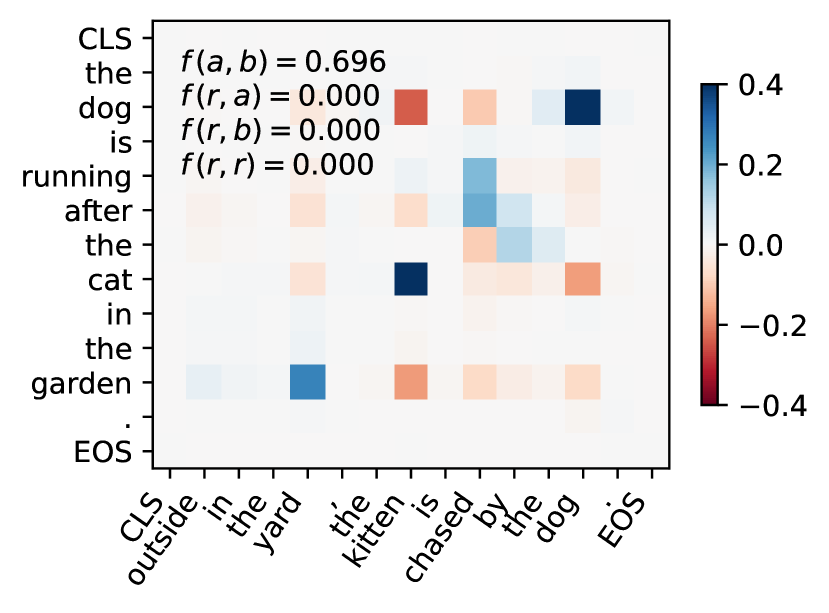
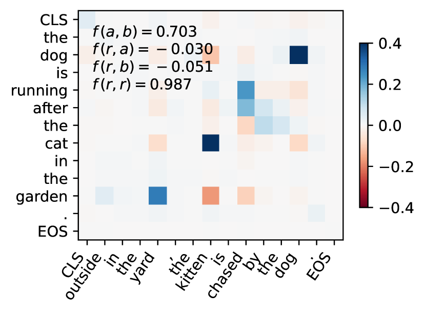
Figure 1: Attributions for the same example in the Exact (top) and Tuned (bottom) models. Plots include individual terms from the LHSs of Equation 2.

To guarantee the side condition of $f(\mathbf{r},\cdot)\!=\!0$, we proposed in Möller et al. (2023) to adjust the model architecture in two ways. First, we shift all embeddings by the references, so that $\mathbf{e}(\cdot)=\mathbf{e}^{\prime}(\cdot)-\mathbf{e}^{\prime}(\mathbf{r})$, where $\mathbf{e}^{\prime}$ is the original encoder and $\,\cdot\,$ is an arbitrary input. This shift results in references to be mapped onto the zero vector in the embedding space, which is why all terms involving r vanish in Equation 2. Unfortunately, Siamese sentence encoders typically use cosine as a similarity measure, which normalizes embedding vectors to unit length. For the zero vector, normalization is undefined. This is why, second, we replace the cosine by a dot product in the previous publication.

The application of these adjustments to a model requires fine-tuning. Thus, attributions cannot be derived for the original model, but only an adapted version of it. The adjustments also result in a slight decrease of predictive performance (cf. row Orig. in Table 1). Finally, a dot-product as similarity measure does not guarantee the similarity of a sentence to itself to be one (i.e. maximal).

3.2 Proposed Extensions

In this work we address these two limitations.

Utilizing cosine similarity.

In Equation 3, the integrated Jacobian $\mathbf{J}_{a}$ results from computing forward- and backward-passes of all interpolation steps $\mathbf{x}(\alpha_{n})$ along the integration path. However, due to the numerical calculation of the integral, the closest input to the reference $\mathbf{r}_{a}$ that is actually ever used is $\mathbf{x}(\alpha)$ with $\alpha\!=\!\|\mathbf{a}-\mathbf{r}_{a}\|/N$, the first interpolation step for input $\mathbf{a}$. For a large number of steps $N$, this input may come arbitrarily close to $\mathbf{r}_{a}$, but never reaches it. Therefore, in practice we actually never need to normalize the zero embedding-vector $\mathbf{e}(\mathbf{r}_{a})$, which $\mathbf{r}_{a}$ is mapped to, and we can safely use cosine as a similarity measure.

Approximate References.

We can loosen the requirement for references to yield exact zero similarities, which allows us to avoid the embedding shift. We still use sequences of padding tokens with the same length as the respective input as references, but we now subtract their emebddings from input embeddings. Padding sequences are nevertheless uninformative and should yield similarities close to zero for most input sentences.

As a result, the last three terms on the left-hand side of Equation 2 do not vanish any more. The two reference similarity terms involving either input will become close to zero: $f(\mathbf{a},\mathbf{r}_{b})\approx 0$ and $f(\mathbf{b},\mathbf{r}_{a})\approx 0$. The reference term will not, but it will become close to one as references should be similar to another, $f(\mathbf{r}_{a},\mathbf{r}_{b})\approx 1$. It may not be exactly one, because if the two inputs are of different lengths, so are the two references, and their sentence representations will not be mapped onto the exact same embedding.

Approximate Attributions.

Combining the approximations from above, we obtain the following approximate attribution method:

$$f(\mathbf{a},\mathbf{b})+1\approx\sum_{ij}\left(\mathbf{a}-\mathbf{r}_{a}\right)_{i}\left(\mathbf{J}^{T}_{a}\mathbf{J}_{b}\right)_{ij}\left(\mathbf{b}-\mathbf{r}_{b}\right)_{j}$$ (4)

The attribution matrix on the right-hand side no longer exactly corresponds to the model prediction, because it is now influenced by the reference term and non-zero reference similarities. A priori, we cannot tell how both contributions distribute among individual feature pairs $ij$, and whether they influence the relative order of attributions. That being said, the ability to utilize cosine similarity and the lack of need for an embedding shift obviates the need for fine-tuning to adjust the model architecture, and Equation 4 offers a means to compute approximate attributions for off-the-shelf models.

4 Experiments 1: Analysis of Attributions

Our approximate attributions do not provide a theoretical guarantee to be correct. Therefore, in this section, after evaluating predictive performances in different settings, we first quantify the influence of reference contributions to approximate attributions, and then evaluate how well exact and approximate attributions agree. We work with attributions to layer nine, because they are expressive, while still being accurate with reasonable computational cost Möller et al. (2023).

4.1 Experimental Setup

We experiment with Siamese sentence transformers trained to predict semantic textual similarity, and base our evaluation on the well-established STS benchmark Cer et al. (2017), consisting of 5749 training, 1500 development and 1379 test sentence pairs from various SemEval tasks. Our implementation builds on the sentence-transformers package (Reimers and Gurevych, 2019). Training details are provided in Appendix A.

4.2 Predictive Performance

We first evaluate the performance of Siamese models on the STS data corresponding to different possible configurations for exact and approximate attributions. The aspects discussed in Section 3.1 give rise to four such configurations, shown in Table 1: they differ in whether we apply an embedding shift (Shift), and whether we train the model on the STS train set (Train). Shelf refers to the unmodified off-the-shelf version. Tuned undergoes the same training as the other fine-tuned models but keeps its unmodified architecture. The Exact model introduces the embedding shift enabling exact attributions. Finally, Orig. is the configuration from Möller et al. (2023) with a dot product as the similarity measure. We evaluate all models on the STS test set using the standard metric of Spearman correlation between the cosine similarity of embeddings and annotations.

The Tuned model achieves the best performance. The Orig. and Exact models sacrifice $1.8$ and $0.3$ points in average correlation, respectively. Using the framework for assessing statistical significance introduced by Dror et al. (2019), the superiority of the Tuned model over the Exact one is, however, not significant ($p\!<\!0.05$, details in Appendix B). This shows that the embedding shift only minimally harms the performance when compared against the unmodified model undergoing identical training (Tuned).

Model	Shift	Train	Attr.	$\mathbf{r_{S}}\!\times 100$
Shelf	✗	✗	appr.	83.4
Tuned	✗	✓	appr.	87.8
Exact	✓	✓	exact	87.5
Orig.	✓	✓	exact	86.0

Table 1: Spearman correlation of cosine similarities between embeddings and target labels in different model settings as described in the text. Top and second best performances are bold / underlined.

Figure 2: Contributions of reference similarities, $f(\mathbf{a},\mathbf{r}_{b})$ and $f(\mathbf{b},\mathbf{r}_{a})$ (left), and the reference term, $f(\mathbf{r}_{a},\mathbf{r}_{b})$ (right), to attributions.

4.3 Reference Contributions

For off-the-shelf models that have not been adapted for the similarities to the references $f(\mathbf{a},\mathbf{r}_{b})$ and $f(\mathbf{b},\mathbf{r}_{a})$ to vanish, we can test how close similarities of inputs to the references actually are. Figure 2 (left) shows the distribution of similarities between all STS test set sentences and corresponding reference inputs consisting of padding tokens. $85.8\%$ of all similarities are within an interval of $\pm 0.1$ around zero. Thus, in many cases the assumption for reference similarities to be negligible, $f(\mathbf{r},\cdot)\approx 0$, may be assumed. However, the width of this distribution also shows that in a substantial fraction of test examples reference similarities are not sufficiently small. Whenever they become non-negligible, they can confound attributions and the approximation of Equation 4 cannot be assumed safely. Fortunately, we can perfectly quantify this error case by case by explicitly computing the reference similarities of both inputs.
Similarly, we can evaluate how large the contribution of the reference term, $f(\mathbf{r}_{a},\mathbf{r}_{b})$, to the attributions is. Figure 2 (right) shows a histogram of all values for this term. As expected, they are mostly close to one. Only $6.7\%$ of all contributions are smaller than $0.9$. Different from the reference similarities for the two inputs, the reference term is never negligible.

4.4 Agreement between Exact and Approximate Attributions

Due to the non-zero reference contributions $f(\mathbf{a},\mathbf{r}_{b})$, $f(\mathbf{b},\mathbf{r}_{a})$ and $f(\mathbf{r}_{a},\mathbf{r}_{b})$, the attribution matrix $\mathbf{A}$ can no longer be assumed to exactly reformulate the model prediction $f(\mathbf{a},\mathbf{b})$, because we cannot tell how the former terms distribute among $\mathbf{A}$ (cf. Equation 2). In order to evaluate how much reference similarities and the reference term confound attributions, we compare approximate attributions from the Tuned model against exact ones from the Exact one. For this evaluation, it is important that both models undergo an identical training, with the only difference being that embeddings in the Exact model are shifted. Therefore, we do not compare attributions of the Shelf or Orig. model in this experiment.

The plots in Figure 1 show example attributions of both models for a random sentence pair from the STS test set. As expected, in the Exact model both reference similarities and the reference term vanish, while in the Tuned one, the former come close to zero and the latter is approximately one. Some attributions are quite different, however, a general pattern appears to be rather well preserved. We evaluate how consistently this is the case by computing attributions from both models for all sentences in the STS test set and compare them. We are also interested how the agreement of attributions behaves as a function of similarity score. In Figure 3, we plot Spearman correlation values of attributions to layer eleven against the average similarity score predicted by the two models. The correlation steadily increases with higher similarity scores. For scores $s\!>\!0.75$ it reaches $r_{S}=0.81\!\pm\!0.07$.

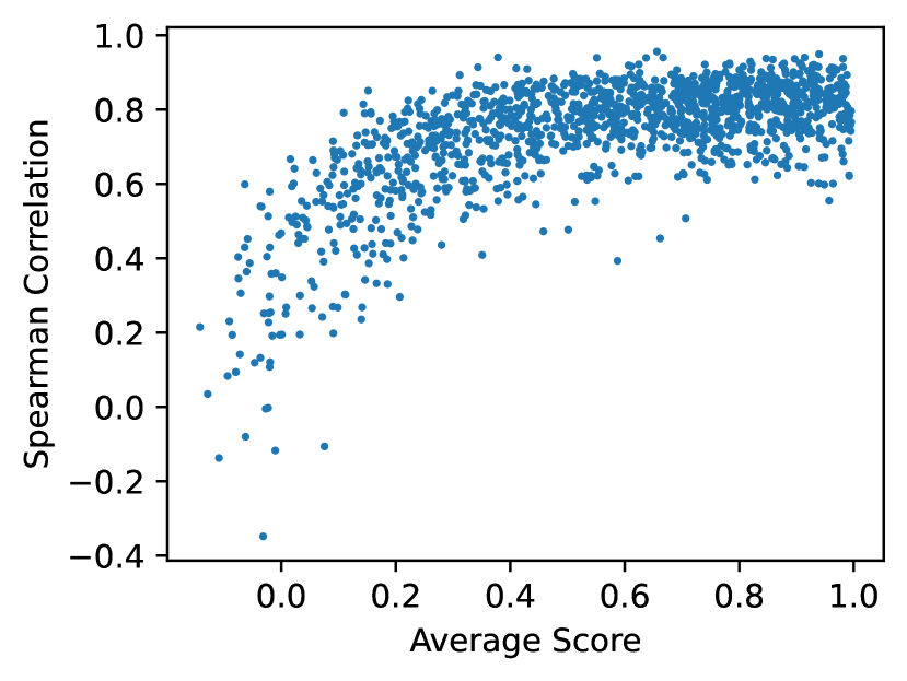
Figure 3: Spearman correlation between attributions from the Tuned and Exact model for all STS test set pairs (y axis) plotted against the mean predicted similarity of both models (x axis).

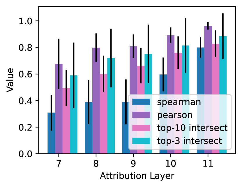
Figure 4: Agreement between attributions by the Tuned and Exact model. We compute Spearman and Pearson correlations, as well as the intersections between the top-3 and top-10 attributions for different layers and similarity scores $s>0.5$.

We repeat this experiment for attributions to all layers down to the seventh, for which we have previously found attributions to be sufficiently accurate with $N\!<\!200$ Möller et al. (2023). Figure 4 summarizes the results for similarity scores $s>0.5$. Spearman correlation declines to $r_{S}=0.60\pm 0.13$ and $r_{S}=0.40\pm 0.17$ in layer ten and nine, respectively. We note that Spearman correlation only regards the rank of attributions and will be strongly influenced by small attributions, which may be dominated by noise and do not interest us very much. Pearson correlation, on the other hand, which remains relatively high with $r_{P}=0.80\pm 0.11$ in layer eight, is technically not suitable because we cannot presuppose a linear relation between attributions. We are mostly interested in the agreement of attributions that stand out. Therefore, we also evaluate the overlap among the top ten (and three, shown in parentheses) attributions in all pairs. The Jaccard coefficient starts at $0.83\!\pm\!0.10$ ($0.88\!\pm\!0.17$) in layer eleven and decreases to $0.60\!\pm\!0.14$ ($0.75\!\pm\!0.20$) in layer eight.

These results show that approximate attributions are trustworthy for very deep layers. Attributions to deeper intermediate representations may still provide interesting insights, but must be interpreted with caution and cannot be taken to be completely reliable. The results also show that care must be applied regarding dissimilar sentence pairs, because for very low scores, approximate attributions do not agree with exact ones.

4.5 Positive and negative attributions

Intuitively, pairs of tokens with congruent semantics, which make a pair of sentences more semantically similar, should positively contribute to the similarity score and receive positive attribution scores. Conversely, pairs of tokens that contradict each other should be assigned negative attributions in order to push the similarity score towards zero, cf. the effect of not in Figure 7. Examination of attribution matrices shows, however, that this scenario is quite rare and we often fail to see noticeable negative attributions where we expect them.

A possible reasons for this behavior is that models tend to “overshoot” the contributions of semantically congruent tokens and need to balance them out by assigning negative contributions to neutral token pairs (unlike the final scores, token-pair contributions can take any value).

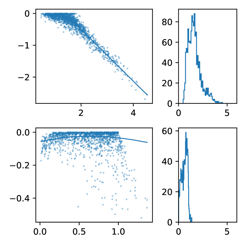
Figure 5: The relationships (with LOWESS smoothing) between sums of positive and negative elements of attribution matrices computed on the STS test set using the Shelf and the Exact model (left pane of top and bottom row, respectively) and the distribution of sums of positive elements in these matrices (right pane).

In order to test if this is the case, we separately extract the sums of all positive and all negative elements of the attribution matrices computed based on the sentence pairs from the STS test set using two similarity models. The relationship between the sums of positive and negative token-pair attributions across sentences is shown in Figure 5. Both models demonstrate cases when positive attributions sum to more than the score maximum, which is 1 for the exact model and 2 for the off-the-shelf model (cf. Equations. 2 and 4), thus demanding a proportional total negative contribution. However, this analysis also shows a difference between the exact model and the approximate model: we see approximate attributions computed on the basis of the off-the-shelf model summing to more than 2 much more frequently than exact attributions summing to more than 1. We cannot tell whether this effect is an artifact of the approximate attribution method or whether the model itself actually assigns such large contributions, while the weights of fine-tuned exact model become normalized. Overall, the data show that, unfortunately, negative attributions are not entirely reliable even in the exact attribution setting, given that positive attributions sometimes sum to more than 1, and in the approximate setting the proportion of these cases is higher.

5 Experiments 2: Analysis of Sentence Transformers

The attributions derived by our method let us directly analyze the decision making process inside STs for the first time. In this section, we extend the analysis to concrete levels of linguistic structures including syntactic functions, negation, adjectives, and general lexical effects.

5.1 Syntactic Relations

Möller et al. (2023) evaluated which relations between parts of speech Siamese language models typically consult. We extend this analysis to relations between the syntactic functions of words. Using a Universal Dependencies parser, we obtain parse trees for all sentence pairs from the STS test set, and replace labels of multi-word expressions and coordinated constructions with the label of their closest parent that is not phrase internal. On the attribution side, we combine token- to word-attributions by averaging. We then extract syntactic relations of the top $10\%$ of all attributions in every sentence pair. Figure 6 shows a distribution of the most attributed relations in our Exact model and the (off-the-) Shelf model.

Figure 6: Distribution of relations between syntactic functions of word-pairs in the top 10% of all attributions for instances in the STS test set.

As one may expect, subject (nsubj), predicate (root marks the predicate of the main clause), direct object (obj), and oblique (obl) relations appear among the top attributions. Notably, top-contributing pairs are based on words with identical syntactic function, which suggests that models begin by matching major syntactic roles before considering mixed relations. Same-function word pairs also show high agreement between models. The two models do not agree so well on attributions to word-pairs of different function. The Exact model tends to attribute to subject–object (nsubj–obj) pairs much more often. The opposite is true for subject–predicate (nsubj–root) relations, which the Shelf model attributes more often than any other mixed relation. In the exact model, somewhat surprisingly, this relation only appears on rank 14.
With a fraction of around $7\%$ subject–subject attributions are by far the most frequent. Nevertheless, this is not a large share of all top attributions, and the rest of the distribution does not decline steeply. Therefore, we can conclude that the models regard a wide range of relations between syntactic roles and do not overly focus on specific ones. At the same time, the relative important of participant-like elements supports that the conclusions reached by Nikolaev and Padó (2023) for synthetic sentences generalize to natural text.

5.2 Negation

It is a well-known fact that sentence transformers do not handle negation well Vahtola et al. (2022). We use our attribution method to seek a deeper understanding of this phenomenon. From the STS test set, we extract 87 sentences that contain a simple not-negation. We then derive attributions for the similarity to the identical but non-negated sentence and compute the total attribution to the not-token.

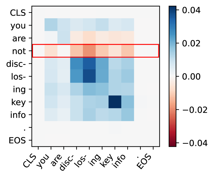
Figure 7: Attribution matrix for a sentence paired with its negation (Exact model). The red box marks the contribution of the negation. This is a rare example of a clear negative contribution (cf. Figure 8).

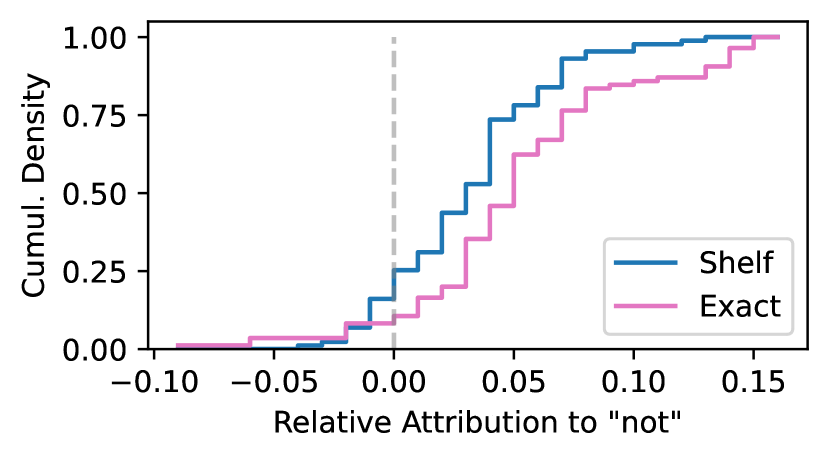
Figure 8: Cumulative distributions of total attributions to the not-token when computing the similarity of a negated sentence to its non-negated version.

The negation should show a negative contribution in the attribution; Figure 7 shows an example where this is actually the case. However, the distribution of attributions in Figure 8 shows that this is not the usual behaviour. In the Shelf (Exact) model only approximately $16\%$ ($9\%$) of all not-attributions are negative. In $90\%$ of the cases relative attributions to the not-token account for less than $8\%$ ($14\%$) of the prediction. This provides additional evidence for the fact that sentence transformers mostly ignore negation.

5.3 Adjectives as Predicates

As another test of the STs’ ability to model polarity, we construct adjective triplets. These combine an anchor adjective with one synonymous and one opposite adjective, e.g. pretty with beautiful and ugly. From a total of 23 such triplets, we then build a synthetic data set consisting of two sentence pairs per triplet (Appendix C) built from the same sentence template. The sentences differ only in the adjective position: One sentence combines the original and the synonymous adjective (This house is beautiful., This house is pretty.), one the original with the opposite one (This house is pretty., This house is ugly.).

We then compute attribution matrices for the two sentence-pairs from every instance, combine token-level to word-level attributions by averaging and evaluate the attributions to the respective adjective pairs. We expect the synonymous pairs to contribute pronounced positive attributions to sentence-similarities. Opposite pairs, on the other hand, result in two sentences with opposing meaning. One may expect that respective adjective-pairs should, hence, receive negative attributions. However, we find that this is not typically the case. In Figure 9, we plot histograms of the attributions to synonymous and opposite adjective pairs for both the Exact and the Shelf model.

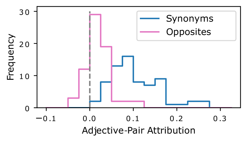
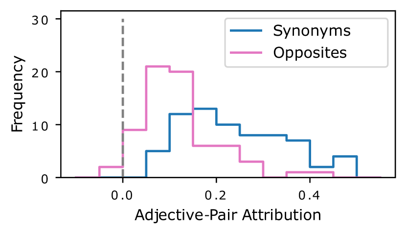
Figure 9: Histograms of attributions to synonymous and opposite adjective pairs from the Exact (top) and the Shelf model (bottom).

In both cases the distributions show that opposite adjective pairs, generally, do receive lower, but only rarely negative attributions.

5.4 Lexical effects

Finally, we investigate whether attributions are lexically biased, i.e. whether similarity scores produced by SEs are sensitive to the exact lexical choice. E.g., given a pair of sentences like A puppy was born in X. vs. How many hurricanes occur in X each year?, intuitively we do not expect the similarity score to noticeably vary with the choice of X. However, the Shelf model predicts scores above 0.3 when X is in Auckland, Cambodia, Granville but only 0.13 for the USA and 0.19 for Europe.

In order to study this more systematically, we use the QQP dataset containing more than 400k question pairs and record values of all matrix cells corresponding to same-token pairs. We then extract all attributions for words appearing 30 and more times and assign them ranks based on their average attributions.

As should be expected, both the Exact model and the Shelf model pay little attention to EOS, CLS, and punctuation signs, which obtain the lowest ranks in both models. As for the top ranks, both models give high ranks to certain place names (Kerala, Pune), words describing emotions (anger, boredom), and a seemingly random assortment of other words corresponding to different question topics (hacking, vocabulary, furniture). Interestingly, while the Exact model also assigns very high importance to particular numbers (2500, 1500, etc.), the Shelf is less sensitive to them (the top number token, 1500, has rank 91). Comparison of ranks for top tokens is shown in Figure 10. Overall, the attribution ranks show high agreement (Spearman’s $r\!=\!0.81$) between the two models, and the standard deviations for the contributions are rather low (cf. Table 3 and 4 and Figure 12 in the appendix), which shows that lexical effects are both strong and consistent.

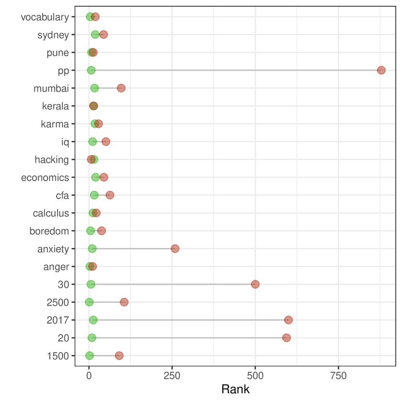
Figure 10: Top-ranking words by their same-token attributions over the QQP dataset sentence pairs. X-axis: ranks (Exact model ranks shown in green, Shelf model ranks in brown).

6 Conclusion

The updates to our original method proposed in this paper (i) result in a Siamese Transformer with exact attribution ability to retain the predictive performance of the equivalent unmodified model, and (ii) enable a way to compute approximate attributions for Siamese encoders which can be directly applied to off-the-shelf models without the need for fine-tuning. Unlike their exact counterparts, these approximate attributions do not come with the theoretical guarantee to exactly reflect the model prediction. Our evaluation, however, shows that for deep intermediate representations they are reliable to a certain extent and often agree with exact attributions.

Analyses carried out based on our attributions show that Siamese transformers primarily match subjects, predicates and objects but also considering different syntactic relations. They mostly do not attend to negation and often assign small yet positive contributions to semantic opposites. On a lexical level, some words always obtain high attributions with small variance whenever they appear.

On the methdological level, we suggest that due to the practicality of approximate attributions, they may be used to obtain a first round of insights into off-the-shelf models. Whenever reliable attributions of predictions are required, however, an exact attribution model should be employed. Therefore, an interesting future perspective will be to train large Siamese models with exact attribution ability from scratch.

7 Limitations

We first emphasize that in this paper a central limitation of our original attribution method for Siamese encoders Möller et al. (2023), namely that a dot-product instead of cosine needs to be used as a similarity measure, is removed. This results in the fact that self-similarity of sentences is guaranteed to be one, instead of being unbound.

The central limitation of approximate attributions for off-the-shelf Siamese Encoders in this paper is that they do not exactly reflect model predictions, which is elaborately discussed above.

A second important limitation remain the high computational costs for attributions to input and shallow intermediate representations. With our available computational resources and the current implementation accurate attributions to shallow layers are not tractable Möller et al. (2023). In the future it will also be important to look into potential options to increase the efficiency for the computation of these attributions.

Finally, deeper intermediate representations in transformer models are contextualized and hence do not represent the associated token alone, but its context. In the future it will also be interesting to investigate the relation between attributions to different layers and contextualization.

Appendix A Training Details

We fine-tune all models in the same way and mostly stick to the default setting that is used in the sentence-transformers package. The batch size is $16$, and wen run all trainings for five epochs. We use an AdamW-optimizer with a weight decay of $0.1$ and learning rate of $2\times 10^{-5}$, taking $10\%$ of the data for linear warm-up.

Appendix B Significance Testing

Dror et al. (2019) introduced a framework that is particularly suitable to test the significance of performance improvements between deep learning models. We apply this test on the distribution of squared errors between predictions and targets on the STS test set (MSE is used as a loss function at training time). We set the tests $\epsilon$-parameter to the suggested value of $\epsilon\!=\!0.3$ and choose a significance level of $p\!<\!0.05$, which is not an overly strict criterion for superiority.

Appendix C Adjective Sentences

Table 2 lists the 23 adjective triplets that we use to construct sentence pairs.

Anchor	Synonym	Opposite
beautiful	pretty	ugly
ugly	hideous	beautiful
small	little	big
big	huge	small
gigantic	enormous	tiny
tiny	minuscule	enormous
old	elderly	young
young	youthful	old
difficult	hard	easy
simple	easy	difficult
thorough	comprehensive	erroneous
faulty	erroneous	thorough
dirty	messy	clean
clean	tidy	dirty
heavy	massive	light
common	normal	unusual
untypical	unusual	normal
boring	dull	interesting
exciting	interesting	boring
calm	peaceful	hectic
chaotic	hectic	calm
balanced	equal	uneven
unequal	uneven	balanced

Table 2: Adjective triplets used for our synthetic dataset

From these triplets we construct sentence tuples like the following: (This house is beautiful., This house is pretty.) and (This house is beautiful., This house is ugly.). Figure 11 shows attribution matrices for this example and marks the adjective attributions that we compare in red.

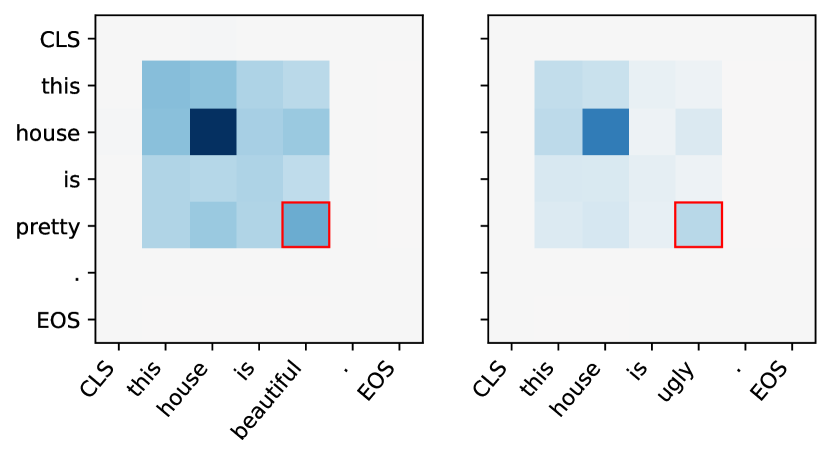
Figure 11: Example attributions for adjective sentences.

Appendix D Lexical Effects

We compute attribution matrices for 148315 sentence pairs at level 8; N = 100. Due to time constraints we could not compute attributions for all sentence pairs for both models. However, we computed them for the Shelf model, and the results are nearly identical to those achieved on the subsample, with Spearman’s $r>0.99$. Top-20 and bottom-20 tokens by average contribution to the similarity score in identical pairs for the two models are shown in Table 3 and 4. Densities of same-token-pair contributions of 30 lexical items with the highest average contribution are shown in Figure 12.

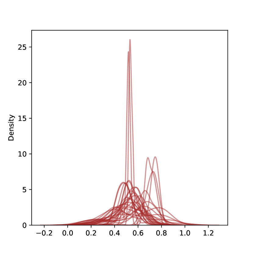
Figure 12: Densities of same-token-pair contributions of 30 lexical items with the highest average contribution.

Word	Mean	StDev
2500	0.399	0.169
1500	0.370	0.116
anger	0.236	0.096
vocabulary	0.218	0.087
boredom	0.216	0.051
30	0.212	0.178
pp	0.212	0.185
pune	0.205	0.110
20	0.203	0.142
anxiety	0.199	0.116
iq	0.191	0.122
calculus	0.190	0.176
2017	0.189	0.090
kerala	0.182	0.067
hacking	0.181	0.105
cfa	0.178	0.120
mumbai	0.174	0.112
karma	0.171	0.086
sydney	0.170	0.100
economics	0.168	0.115
very	0.003	0.005
described	0.003	0.003
(	0.003	0.004
	0.003	0.004
"	0.003	0.004
hear	0.003	0.004
because	0.003	0.003
)	0.002	0.003
,	0.002	0.003
.	0.002	0.005
@	0.002	0.009
ones	0.002	0.001
[	0.002	0.003
{	0.001	0.001
]	0.001	0.001
_	0.001	0.001
\	0.001	0.001
}	0.001	0.001
EOS	0.000	0.000
CLS	0.000	0.000

Table 3: Top-20 and bottom-20 tokens by average contribution to the similarity score in identical pairs. Values for level 8 of the Exact model.

Word	Mean	StDev
auckland	0.737	0.045
cambodia	0.713	0.098
somme	0.656	0.087
sahara	0.533	0.079
shotgun	0.514	0.032
surgical	0.507	0.127
hacking	0.503	0.143
swiss	0.502	0.116
turkey	0.496	0.150
edmonton	0.490	0.068
anger	0.477	0.093
##oop	0.477	0.168
pune	0.472	0.124
kerala	0.461	0.084
goa	0.455	0.113
coding	0.455	0.169
wikipedia	0.454	0.116
enfield	0.453	0.114
vocabulary	0.449	0.086
furniture	0.447	0.103
their	0.008	0.009
’	0.007	0.006
the	0.007	0.007
that	0.007	0.007
"	0.005	0.009
those	0.005	0.011
[	0.004	0.010
(	0.004	0.010
@	0.004	0.026
	0.004	0.005
,	0.002	0.004
ones	0.002	0.004
{	0.002	0.004
)	0.002	0.006
\	0.001	0.001
_	0.001	0.002
]	0.001	0.001
}	0.000	0.000
CLS	0.000	0.001
EOS	0.000	0.000

Table 4: Top-20 and bottom-20 tokens by average contribution to the similarity score in identical pairs. Values for level 8 of the Shelf model.

References

- Atanasova et al. (2020) Pepa Atanasova, Jakob Grue Simonsen, Christina Lioma, and Isabelle Augenstein. 2020. A diagnostic study of explainability techniques for text classification. In Proceedings of the 2020 Conference on Empirical Methods in Natural Language Processing (EMNLP), pages 3256–3274, Online. Association for Computational Linguistics.
- Bastings and Filippova (2020) Jasmijn Bastings and Katja Filippova. 2020. The elephant in the interpretability room: Why use attention as explanation when we have saliency methods? In Proceedings of the Third BlackboxNLP Workshop on Analyzing and Interpreting Neural Networks for NLP, pages 149–155, Online. Association for Computational Linguistics.
- Cer et al. (2017) Daniel Cer, Mona Diab, Eneko Agirre, Iñigo Lopez-Gazpio, and Lucia Specia. 2017. SemEval-2017 task 1: Semantic textual similarity multilingual and crosslingual focused evaluation. In Proceedings of the 11th International Workshop on Semantic Evaluation (SemEval-2017), pages 1–14, Vancouver, Canada. Association for Computational Linguistics.
- Clark et al. (2019) Kevin Clark, Urvashi Khandelwal, Omer Levy, and Christopher D. Manning. 2019. What does BERT look at? an analysis of BERT’s attention. In Proceedings of the 2019 ACL Workshop BlackboxNLP: Analyzing and Interpreting Neural Networks for NLP, pages 276–286, Florence, Italy. Association for Computational Linguistics.
- Conneau et al. (2017) Alexis Conneau, Douwe Kiela, Holger Schwenk, Loïc Barrault, and Antoine Bordes. 2017. Supervised learning of universal sentence representations from natural language inference data. In Proceedings of the 2017 Conference on Empirical Methods in Natural Language Processing, pages 670–680, Copenhagen, Denmark. Association for Computational Linguistics.
- Danilevsky et al. (2020) Marina Danilevsky, Kun Qian, Ranit Aharonov, Yannis Katsis, Ban Kawas, and Prithviraj Sen. 2020. A survey of the state of explainable AI for natural language processing. In Proceedings of the 1st Conference of the Asia-Pacific Chapter of the Association for Computational Linguistics and the 10th International Joint Conference on Natural Language Processing, pages 447–459, Suzhou, China. Association for Computational Linguistics.
- Doshi-Velez and Kim (2017) Finale Doshi-Velez and Been Kim. 2017. Towards a rigorous science of interpretable machine learning. arXiv:1702.08608.
- Dror et al. (2019) Rotem Dror, Segev Shlomov, and Roi Reichart. 2019. Deep dominance - how to properly compare deep neural models. In Proceedings of the 57th Annual Meeting of the Association for Computational Linguistics, pages 2773–2785, Florence, Italy. Association for Computational Linguistics.
- Kobayashi et al. (2024) Goro Kobayashi, Tatsuki Kuribayashi, Sho Yokoi, and Kentaro Inui. 2024. Analyzing feed-forward blocks in transformers through the lens of attention map. In Proceedings of the Twelfth International Conference on Learning Representations, Vienna, Austria.
- Li et al. (2016) Jiwei Li, Xinlei Chen, Eduard Hovy, and Dan Jurafsky. 2016. Visualizing and understanding neural models in NLP. In Proceedings of the 2016 Conference of the North American Chapter of the Association for Computational Linguistics: Human Language Technologies, pages 681–691, San Diego, California. Association for Computational Linguistics.
- MacAvaney et al. (2022) Sean MacAvaney, Sergey Feldman, Nazli Goharian, Doug Downey, and Arman Cohan. 2022. ABNIRML: Analyzing the behavior of neural IR models. Transactions of the Association for Computational Linguistics, 10:224–239.
- Murdoch et al. (2019) W James Murdoch, Chandan Singh, Karl Kumbier, Reza Abbasi-Asl, and Bin Yu. 2019. Definitions, methods, and applications in interpretable machine learning. Proceedings of the National Academy of Sciences, 116(44):22071–22080.
- Möller et al. (2023) Lucas Möller, Dmitry Nikolaev, and Sebastian Padó. 2023. An attribution method for Siamese encoders. In Proceedings of the 2023 Conference for Empirical Methods in Natural Language Processing, pages 15818–15827, Singapore. Association for Computational Linguistics.
- Nikolaev and Padó (2023) Dmitry Nikolaev and Sebastian Padó. 2023. Representation biases in sentence transformers. In Proceedings of the 17th Conference of the European Chapter of the Association for Computational Linguistics, pages 3701–3716, Dubrovnik, Croatia. Association for Computational Linguistics.
- Opitz and Frank (2022) Juri Opitz and Anette Frank. 2022. SBERT studies meaning representations: Decomposing sentence embeddings into explainable semantic features. In Proceedings of the 2nd Conference of the Asia-Pacific Chapter of the Association for Computational Linguistics and the 12th International Joint Conference on Natural Language Processing (Volume 1: Long Papers), pages 625–638, Online only. Association for Computational Linguistics.
- Qi et al. (2020) Peng Qi, Yuhao Zhang, Yuhui Zhang, Jason Bolton, and Christopher D. Manning. 2020. Stanza: A Python natural language processing toolkit for many human languages. In Proceedings of the 58th Annual Meeting of the Association for Computational Linguistics: System Demonstrations.
- Reimers and Gurevych (2019) Nils Reimers and Iryna Gurevych. 2019. Sentence-BERT: Sentence embeddings using Siamese BERT-networks. In Proceedings of the 2019 Conference on Empirical Methods in Natural Language Processing and the 9th International Joint Conference on Natural Language Processing (EMNLP-IJCNLP), pages 3982–3992, Hong Kong, China. Association for Computational Linguistics.
- Rogers et al. (2020) Anna Rogers, Olga Kovaleva, and Anna Rumshisky. 2020. A primer in BERTology: What we know about how BERT works. Transactions of the Association for Computational Linguistics, 8:842–866.
- Rudin (2019) Cynthia Rudin. 2019. Stop explaining black box machine learning models for high stakes decisions and use interpretable models instead. Nature machine intelligence, 1(5):206–215.
- Sundararajan et al. (2017) Mukund Sundararajan, Ankur Taly, and Qiqi Yan. 2017. Axiomatic attribution for deep networks. In Proceedings of the 34th International Conference on Machine Learning - Volume 70, page 3319–3328. JMLR.org.
- Thakur et al. (2021) Nandan Thakur, Nils Reimers, Andreas Rücklé, Abhishek Srivastava, and Iryna Gurevych. 2021. BEIR: A heterogeneous benchmark for zero-shot evaluation of information retrieval models. In Thirty-fifth Conference on Neural Information Processing Systems Datasets and Benchmarks Track (Round 2).
- Vahtola et al. (2022) Teemu Vahtola, Mathias Creutz, and Jörg Tiedemann. 2022. It is not easy to detect paraphrases: Analysing semantic similarity with antonyms and negation using the new SemAntoNeg benchmark. In Proceedings of the Fifth BlackboxNLP Workshop on Analyzing and Interpreting Neural Networks for NLP, pages 249–262, Abu Dhabi, United Arab Emirates (Hybrid). Association for Computational Linguistics.
- Voita et al. (2019) Elena Voita, David Talbot, Fedor Moiseev, Rico Sennrich, and Ivan Titov. 2019. Analyzing multi-head self-attention: Specialized heads do the heavy lifting, the rest can be pruned. In Proceedings of the 57th Annual Meeting of the Association for Computational Linguistics, pages 5797–5808, Florence, Italy. Association for Computational Linguistics.
- Wiegreffe and Pinter (2019) Sarah Wiegreffe and Yuval Pinter. 2019. Attention is not not explanation. In Proceedings of the 2019 Conference on Empirical Methods in Natural Language Processing and the 9th International Joint Conference on Natural Language Processing (EMNLP-IJCNLP), pages 11–20, Hong Kong, China. Association for Computational Linguistics.