The Gaia RVS benchmark stars
II. A sample of stars selected for their Gaia high radial velocity

Abstract

Context. The Gaia satellite has already provided the astronomical community with three data releases, and the Radial Velocity Spectrometer (RVS) on board Gaia has provided the radial velocity for 33 million stars.

Aims. When deriving the radial velocity from the RVS spectra, several stars are measured to have large values. To verify the credibility of these measurements, we selected some bright stars with the modulus of radial velocity in excess of 500 $\rm kms^{-1}$ to be observed with SOPHIE at OHP and UVES at VLT. This paper is devoted to investigating the chemical composition of the stars observed with UVES.

Methods. We derived atmospheric parameters using Gaia photometry and parallaxes, and we performed a chemical analysis using the MyGIsFOS code.

Results. We find that the sample consists of metal-poor stars, although none have extremely low metallicities. The abundance patterns match what has been found in other samples of metal-poor stars selected irrespective of their radial velocities. We highlight the presence of three stars with low Cu and Zn abundances that are likely descendants of pair-instability supernovae. Two stars are apparently younger than 1 Ga, and their masses exceed twice the turn-off mass of metal-poor populations. This makes it unlikely that they are blue stragglers because it would imply they formed from triple or multiple systems. We suggest instead that they are young metal-poor stars accreted from a dwarf galaxy. Finally, we find that the star RVS721 is associated with the Gjoll stream, which itself is associated with the Globular Cluster NGC 3201.

1 Introduction

Since 2014 the Gaia satellite (Gaia Collaboration et al., 2016b) has provided crucial information (most important positions, parallaxes, proper motions, radial velocities, and stellar parameters) for a huge sample of stars. Since its launch, there have been three data releases (DR1, DR2, DR3; Gaia Collaboration et al., 2016a, 2018, 2022).

The data provided in the Gaia releases have been used by the astronomical community to improve our knowledge on the Milky Way and the Local Group galaxies. There are still limitations on the data provided by Gaia, such as a limitation in brightness, and in this respect, there is nothing that can be done to overcome it. But there are things that can be improved. In Caffau et al. (2021), we presented a project to build an archive of Gaia Radial Velocity Spectrometer (RVS) benchmark stars, acquiring high-quality spectra to be used to derive the line spread function of stars observed by the Gaia RVS and to provide reference stars for the radial velocity ($V_{\mathrm{r}}$) determination in as many focal plane positions as possible. In this way, we had the goal of improving the $V_{\mathrm{r}}$ determination from the RVS spectra. The project is still open, and the spectra observed will be used in the Gaia data releases 4 and 5. Nine of the stars investigated in this work (RVS701, RVS702, RVS703, RVS706, RVS707, RVS714, RVS719, RVS720) have spectra of sufficient quality in the RVS wavelength range and will be added into the archive of Gaia RVS benchmark stars.

This project also gives us the opportunity to investigate other possible problems for the $V_{\mathrm{r}}$ measurements from the RVS spectra. The RVS spectra have a wavelength range of less than 30 nm, and several spectra have a low signal-to-noise ratio (S/N); in fact, a considerable fraction (about 25%) of $V_{\mathrm{r}}$ determination in the Gaia DR3 derives from spectra with $\rm S/N<5$ (see Katz et al., 2023). These facts, especially the latter, introduce a limitation for a good $V_{\mathrm{r}}$ determination. We also found in the Gaia DR 3 that there are stars with extreme $V_{\mathrm{r}}$, and it is unclear whether these values are real or just evidence of problematic spectra. To verify the extreme $V_{\mathrm{r}}$ values and confirm or discard them, we added a sample of extreme $V_{\mathrm{r}}$ stars in the project focused on observing the Gaia RVS benchmark stars. The kinematic investigation of the sample is to be presented by Katz et al. (in preparation). In this work, we show the results of our chemical investigation.

Another intriguing fact of this high $V_{\mathrm{r}}$ sample is that these stars are surely high-speed stars, and it is indeed interesting to combine kinematic and chemical characteristics of high-speed stars. Caffau et al. (2020) investigated a sample of stars selected in Gaia DR 2 for their high transverse velocity, so still high-speed stars. In their sample, some stars happen to appear younger than 6 Ga. This is an intriguing finding that could be explained by a population of blue straggler stars. From a similar selection from Gaia DR3, Bonifacio et al. (2024) highlighted a metal-poor, apparently young population barely compatible with blue straggler stars because their masses are in excess of twice the mass of a typical turn-off metal-poor star and in excess of typical masses of blue stragglers in galactic globular clusters and in the field. We questioned whether we would also find this apparently young population in high $V_{\mathrm{r}}$ stars. The answer we derived is positive, and the two young stars detected in this work are unlikely to be blue stragglers because their masses are in excess of $\rm 1.9M_{\odot}$, while blue straggler stars typically have masses $\rm<1.2\ to\ 1.5M_{\odot}$ (see e.g. Carney et al., 2005; Fiorentino et al., 2014; Ferraro et al., 2023).

2 Target selection

The targets we selected from the Gaia EDR3 (Gaia Collaboration et al., 2021) and Gaia DR3 (Gaia Collaboration et al., 2022) catalogues are stars with an absolute radial velocity in excess of 500 $\rm kms^{-1}$. Overall, we wanted to verify whether these large values are mistakes of the pipeline or that the stars really have a large radial velocity.

We made a similar selection of targets regarding a sample of stars observed with SOPHIE at Observatoire de Haute-Provence (OHP). The SOPHIE sample and the kinematic analysis of this sample are discussed in Katz et al. (in preparation). As stated in Katz et al. (in preparation), the stars observed with UVES and investigated in this work are high $V_{\mathrm{r}}$ stars. The Gaia G magnitude in the sample is in the range from 10.2 to 13.6 mag.

3 Observations

A sample of 45 stars was observed in the ESO programme 0109.22XP.001 with UVES (Dekker et al., 2000) at VLT in the setting DIC2 437+760 (wavelength ranges 373-499 and 565-946 nm), with slit 0$\aas@@fstack{\prime\prime}$4 (resolving power 90 000) in the blue arm and 0$\aas@@fstack{\prime\prime}$3 (resolving power 110 000) in the red arm. A single exposure of about half an hour was taken for each star. A sub-sample of 19 stars were re-observed in ESO programme 110.23V0.001.

Of the observations in P109, 42 were graded ’A’ and three ’B’. In P110, of the 21 spectra investigated, 17 were graded ’A’ and four ’B’. For the star RVS735, observed in P109, there is no blue spectrum.

For the stars of P109, we downloaded the UVES spectra reduced by ESO in order to have an homogeneous data reduction and to make data readily available to the community. The spectra of four stars are shown in Fig. 1 in the wavelength range of Gaia RVS. Few stars showed problems in the data reduction, and we reduced the spectra by using the ESO pipeline. For P110, we reduced the spectra to have quick access to them.

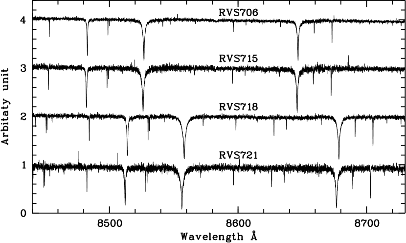
Figure 1: Four spectra shown in the wavelength range of the Gaia RVS.

We performed the chemical analysis of 43 stars. Regarding the two stars for which there is no chemical analysis, the spectrum of RVS705 is noisy (S/N is too low) and crowded due to it being a carbon star (Alksnis et al., 2001). The second star, RVS724, is a variable and active star whose two spectra are different (see Fig. 2). For the stars with observations in P109 and P110, we added the spectra, except for RVS712 and RVS736, which showed clear differences in radial velocity.

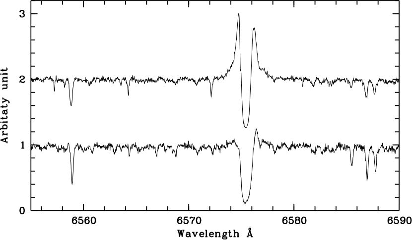
Figure 2: Two observations of RVS724.

4 Analysis

The kinematic investigation of this sample of stars is presented in Katz et al. (in preparation). The stars investigated in this work all belong to the Galactic halo according to the criteria by Bensby et al. (2014).

For the chemical investigation, we needed the spectrum to be at laboratory wavelength. We applied the radial velocity provided by Gaia DR3. All the stars we investigated have been confirmed to have a high radial velocity. For the majority of them, the velocity we derived is within a few kilometres per second from the value provided by Gaia DR3. Just one star, RVS739, shows a disagreement between the two velocities, by about 10 $\rm kms^{-1}$, but the star is still a high $V_{\mathrm{r}}$ star. Our pipeline MyGIsFOS for the chemical investigation was allowed to shift each feature by half of the total broadening of the grid used in the analysis of each star. We verified that the shift applied by MyGIsFOS was sufficient to investigate all the features. If it was not, we applied an extra shift to the spectrum.

4.1 Stellar parameters

To derive the stellar parameters, we used the Gaia DR3 photometry and parallax and the reddening from Vergely et al. (2022). We derived the parallax zero-point as suggested by Lindegren et al. (2021). We first de-reddened the Gaia $G,G_{BP}$, and $G_{RP}$ photometry by using the maps provided by Vergely et al. (2022) and the theoretical extinction coefficients derived from model atmospheres (Mucciarelli & Bonifacio in preparation). The $G_{BP}-G_{RP}$ Gaia DR3 colours were then compared to the synthetic photometry in order to derive the effective temperature. The gravity was derived by using the parallax, corrected by the zero-point, through the Stefan-Boltzmann equation. We first assumed a solar metallicity and derived for each star the effective temperature, $T\rm_{eff}$, and surface gravity, $\log\,g$.

The initial stellar parameters were used to derive the metallicity of the stars by using MyGIsFOS (Sbordone et al., 2014). The metallicity derived in this way was then used to derive new stellar parameters. The iterations were repeated up to when the changes in $T\rm_{eff}$ and $\log\,g$ were within 10 K and 0.02 dex, respectively. The micro-turbulence ($\xi$) was derived by using the calibration of Mashonkina et al. (2017). For the majority of the stars in the sample, the signal-to-noise ratio of the spectra is in fact too low to allow the use of lines with small equivalent widths in order to derive the micro-turbulence by the balance of A(Fe) derived from Fe i lines of different equivalent widths.

Regarding the derivation of the stellar parameters, the grid of synthetic photometry was limited, and we did not allow any extrapolation in $T\rm_{eff}$ or $\log\,g$ beyond the grid. The lower limit accepted in $T\rm_{eff}$ is 4000 K. Six stars converge at this lower-limit in $T\rm_{eff}$ when deriving the stellar parameters, so one could suppose that these stars are in fact cooler. For all these stars (RVS708, RVS714, RVS719, RVS727, RVS730, and RVS734) the calibration of Mucciarelli et al. (2021) provides values close to 4000 K, so we expected that by adopting 4000 K, the stellar $T\rm_{eff}$ would be well within the uncertainty.

If we had used the distance estimate of Bailer-Jones et al. (2021) provided in Gaia DR3 to derive the stellar parameters instead of the parallax corrected by the zero-point, we would have derived $T\rm_{eff}$ as being, on average, 6 K hotter (with a difference always within 40 K) and an average difference in $\log\,g$ of –0.07 dex (with a maximum value at –0.21 dex). These changes in the stellar parameters would not have affected the metallicity derived from Fe i lines (generally well within 0.1 dex and 0.02 dex for $T\rm_{eff}$ and $\log\,g$, respectively) and would have only marginally affected (within 0.1 dex) the iron ionisation balance because the Fe abundance, when derived from Fe ii, is sensitive to the surface gravity.

When comparing our adopted stellar parameters ($T\rm_{eff}$ and $\log\,g$) to the parameters derived by using the calibration of Mucciarelli et al. (2021), we found an average difference in $T\rm_{eff}$ of $-73\pm 37$ K and in $\log\,g$ of $-0.03\pm 0.02$ dex. We adopted 100 K as the uncertainty in $T\rm_{eff}$ and 0.1 dex in $\log\,g$.

In Fig. 3, a comparison of the adopted stellar parameters to PARSEC isochrones (Bressan et al., 2012; Marigo et al., 2017) is shown. In the figure we noted that at least two stars (RVS725 and RVS726), which are both very metal poor, appear younger than expected when compared to the isochrones. When comparing the $G_{BP}-G_{RP}$ colour and the $G$ absolute magnitude to isochrones of various ages, depending on the evolutionary stage, the possible expected masses and ages for RVS725 are $\rm 3.2M_{\odot}$ with age of 230 Ma (as a sub-giant branch or a Hertzsprung gap for more intermediate and massive stars), $\rm 2.9M_{\odot}$ with age of 280 Ma (still core He-burning, the blueward part of the Cepheid loop of intermediate and massive stars), $\rm 2.6M_{\odot}$ with age of 390 Ma (the early asymptotic giant branch or a quick stage of red giant for massive stars). For RVS726 we have just one solution in the interpolation, which is $\rm 1.9M_{\odot}$ with age of 900 Ma (the early asymptotic giant branch or a quick stage of red giant for massive stars). A mass below about $\rm 1.8M_{\odot}$ can in principle be acceptable for a star to be a blue straggler that is the result of the merging of two old metal-poor stars. However, one has to assume no mass was lost in the merging process. The mass expected for RVS725 is far too large. For both stars, to derive the masses and ages, we used a PARSEC isochrone of metallicity of $-1.95$ (we emphasise that PARSEC isochrones are not enhanced in $\alpha$ elements, and for this reason, we selected a metallicity that was slightly higher than the [Fe/H] derived for the two stars, which are $\alpha$-enhanced) and ages from 100 Ma and 3 Ga with a step of 200 Ma. An isochrone at metallicity $-1.65$ dex would provide the same result or increase the masses by less than $\rm 0.1M_{\odot}$. We concluded that these two stars, but especially RVS725, can really be young stars and were probably formed in dwarf galaxies in a recent time and then accreted.

Table 1: Solar abundances.

Element	A(X)	Reference
C	8.50	Caffau et al. (2011)
O	8.76	Caffau et al. (2011)
Na	6.30	Lodders et al. (2009)
Mg	7.54	Lodders et al. (2009)
Al	6.47	Lodders et al. (2009)
Si	7.52	Lodders et al. (2009)
S	7.16	Caffau et al. (2011)
Ca	6.33	Lodders et al. (2009)
Sc	3.10	Lodders et al. (2009)
Ti	4.90	Lodders et al. (2009)
V	4.00	Lodders et al. (2009)
Cr	5.64	Lodders et al. (2009)
Mn	5.37	Lodders et al. (2009)
Fe	7.52	Caffau et al. (2011)
Co	4.92	Lodders et al. (2009)
Ni	6.23	Lodders et al. (2009)
Cu	4.21	Lodders et al. (2009)
Zn	4.62	Lodders et al. (2009)
Y	2.21	Lodders et al. (2009)
Eu	0.52	Lodders et al. (2009)
Ba	2.17	Lodders et al. (2009)

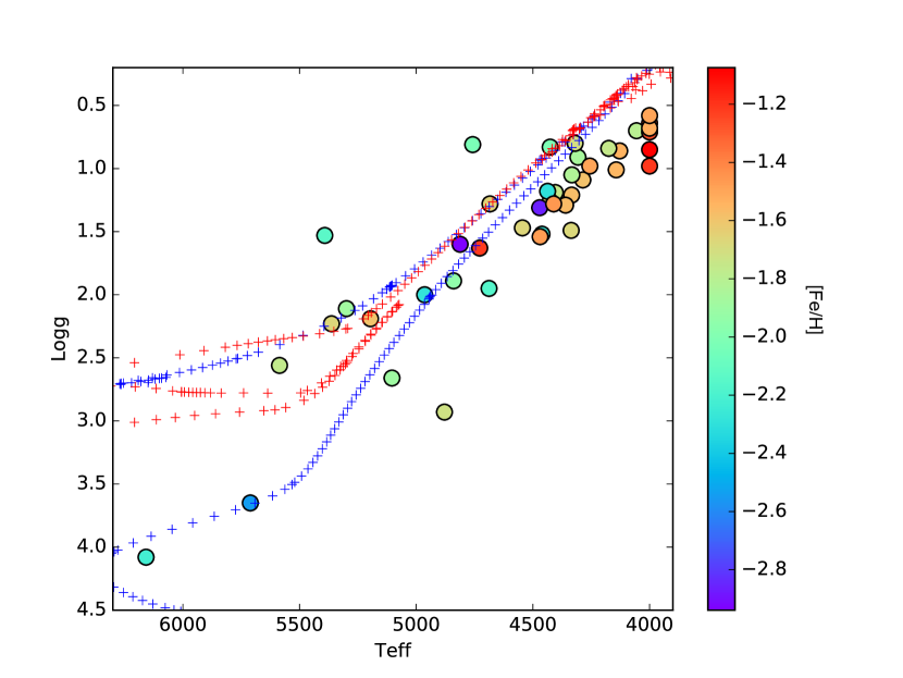
Figure 3: Observed stars in the ($T\rm_{eff}$,$\log\,g$) diagram compared to PARSEC isochrones of metallicity –1.5 dex and of ages 12 Ga (blue crosses) and 1 Ga (red crosses), to guide the eye. The [Fe/H] of the stars are colour coded according the vertical bar on the left.

The stars analysed in this work are all metal poor ($\rm[Fe/H]<-1.0$), but no star is extremely metal poor ($\rm[Fe/H]<-3$). We recall that RVS705 is metal rich, but this star has not been analysed. The stellar parameters and the abundances derived are provided at CDS in an online table that is described in the appendix.

Table 2: Signal-to-noise ratio of the spectra.

Star	ID Gaia DR3	Period	S/N
			@600 nm
RVS700	3064774107059078784	109	75
RVS701	6148919860947868160	109+110	78
RVS702	5654083549060480256	109	66
RVS703	4585522112754440576	109	82
RVS704	4567509294790548096	109	68
RVS705	5641794449335693184	109	$<$20
RVS706	1772048878641647488	109+110	76
RVS707	6102498720545983744	109+110	65
RVS708	4087001612275854976	109	38
RVS709	1774647123402000896	109	32
RVS710	2831494371421184512	109	24
RVS711	5806001524479916160	109+110	37
RVS712	5843949763886962304	109	34
RVS712	5843949763886962304	110	49
RVS713	2731609959149919360	109	40
RVS714	1789332097623284736	109	45
RVS715	4200211044628918016	109	23
RVS716	3545088275525629312	109+110	42
RVS718	5430581735975161344	109+110	44
RVS719	4048087421869545216	109+110	46
RVS720	4292051361144994304	109	27
RVS721	5365576065922008960	109+110	26
RVS722	5932387366845310208	109	32
RVS723	3830347565099377152	109+110	67
RVS724	5354656541072512000	109
RVS725	5860126260025908992	109	8
RVS726	5515555464906936192	109	15
RVS727	4052560510049395840	109+110	40
RVS728	3585461964540660224	109+110	36
RVS729	4434477664957276544	109+110	26
RVS730	1761871661577694848	109	26
RVS731	1751668601691825664	109	19
RVS732	4532552345513094144	109	10
RVS733	3572878053960750976	109+110	51
RVS734	4207775547189676160	109+110	28
RVS735	2697864023148222976	109	14
RVS736	5806698825316687872	109	22
RVS736	5806698825316687872	110	18
RVS737	6418433113222352000	109+110	26
RVS738	1876742967089592448	109	20
RVS739	1775026115611202560	109	21
RVS740	6103440486613002496	109+110	51
RVS741	4219344020113924096	109	17
RVS742	1803730786507192448	109	24
RVS743	4638362923593318912	109	29
RVS744	2689355276322100224	109	18
RVS745	5803679463301298944	109+110	25

4.2 Abundances

The abundances were derived by MyGIsFOS (Sbordone et al., 2014). The solar reference abundances are listed in Table 1. The synthetic spectra grids are the same as described in Caffau et al. (2021).

Lithium is clearly visible in the metal-poor turn-off star RVS738, providing $\rm A(Li)_{\rm LTE}=2.34$. Three evolved stars (RVS702, RVS706, RVS711) show a feature at the wavelength position of the Li 670 nm doublet, and the Li abundance derived from this feature is low ($\rm A(Li)_{\rm LTE}$ of –0.30, 1.07 and 0.89, respectively).

For some elements, we compared the observed spectrum to a grid of synthetic spectra, computed with SYNTHE from an ATLAS 9 model (Kurucz, 2005) while only varying the abundance of one element. We minimised the $\chi^{2}$ to derive the abundance.

We investigated the G-band at 430 nm formed by CH lines to verify if any of the stars was a carbon-enhanced metal-poor (CEMP) star. Through line profile fitting, we could derive the C abundance for 39 stars in the sample, and none appeared to be rich in carbon. We found nearly all stars but one have a negative or close to zero [C/Fe] ratio, in agreement with the results by Spite et al. (2005). These stars are all evolved, and the carbon destruction is due to their stellar evolution. The turn-off star RVS738, as expected and described in Bonifacio et al. (2009), shows a C enhancement: $\rm[C/Fe]=+0.25\pm 0.25$. In Fig. 4, the [C/Fe] ratio is plotted against the surface gravity. We expected that more evolved stars would have converted more C into N, but things are more complicated than that. The trend is not evident, and an extra-mixing should be present, though different in the various stars, in order to favour C destruction. We also expected at least a fraction of the stars to be CEMP stars, but we found none. In this metallicity regime (Bonifacio et al., 2015), we expected that CEMP stars would lie on the high C band described by Spite et al. (2013), with a carbon abundance just below solar. So [C/Fe] would still be positive even if the evolution of the CEMP stars had destroyed part of their carbon.

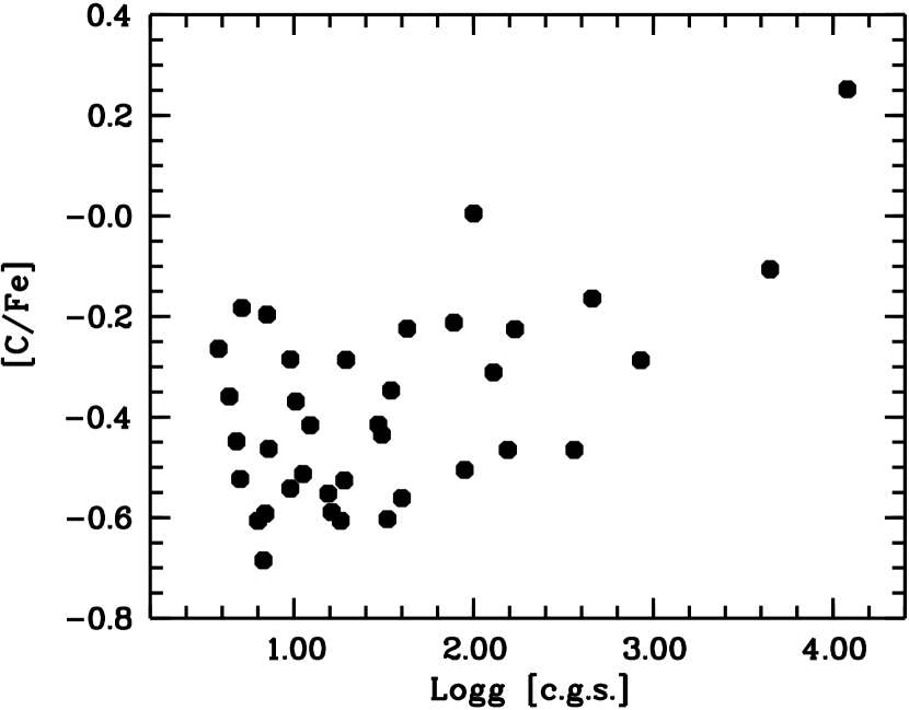
Figure 4: [C/Fe] versus $\log\,g$ for the observed sample.

Oxygen was derived by line profile fitting because the region is contaminated by telluric absorptions. We derived A(O) from the [OI] lines for 26 stars in the sample. All the stars in the sample are enhanced in oxygen, with $\rm\langle[O/Fe]\rangle=0.60\pm 0.11$, which is consistent with the results by Spite et al. (2005), and the star with the highest oxygen value was RVS733, $\rm[O/Fe]=0.92$.

The stars in the sample are enhanced in the $\alpha$ elements, as expected in metal-poor stars (see Fig. 5). The corrections for departures from local thermodynamic equilibrium (NLTE) for Mg and Si in this sample of stars are not large (see Matas Pinto et al., 2022; Caffau et al., 2023). The star RVS726 has a low [Si/Fe] ratio ($\rm[Si/Fe]=-0.21$), lower than the other $\alpha$ elements, which are still low. The strong S i lines of Mult. 1 at 920 nm fall in the REDU CCD, but the region is unfortunately contaminated by telluric absorption. We then carefully inspected the analysis done by MyGIsFOS and rejected the problematic lines. We then derived A(S) for nine stars. After applying the NLTE corrections on [S/H] from Takeda et al. (2005), two stars were found to have a negative [S/Fe]: $\rm[S/Fe]=-0.05$ for RVS703 (based on one single line) and $\rm[S/Fe]=-0.25$ for RVS712 (based on two lines with a relatively high scatter of 0.25 dex). We investigated several Ca i lines to derive the Ca abundance. The line-to-line scatter is generally small ($\rm\langle\sigma\rangle=0.10\pm 0.03$), as expected from the S/N ratios of the spectra. The NLTE corrections as provided by Mashonkina et al. (2016) are on the order of 0.1 dex. When deriving the NLTE corrections for the Ca i for each star for lines used and available in Mashonkina et al. (2007), we derived an average NLTE correction on A(Ca) of 0.10 dex.

For the complete sample of stars for which we performed the chemical investigation (43 stars), we derived $\rm\langle[Ca/Fe]\rangle=0.34\pm 0.08$. For 41 of these stars, we derived an Mg abundance $\rm\langle[Mg/Fe]\rangle=0.42\pm 0.10$. Removing the four stars with a consistently low Mg and Ca (RVS708, RVS709, RVS726 and RVS745), we derived $\rm\langle[Ca/Fe]\rangle=0.35\pm 0.06$ and $\rm\langle[Mg/Fe]\rangle=0.44\pm 0.08$, and the star-to-star scatter was reduced. The star RVS708 also has low [Na/Fe] and [Al/Fe] ratios. The star RVS709 has low [Na/Fe], [Si/Fe], [Y/Fe], and [Zn/Fe] ratios and a slightly low [Al/Fe]. The star RVS726 has low [Na/Fe] and [Si/Fe] ratios.

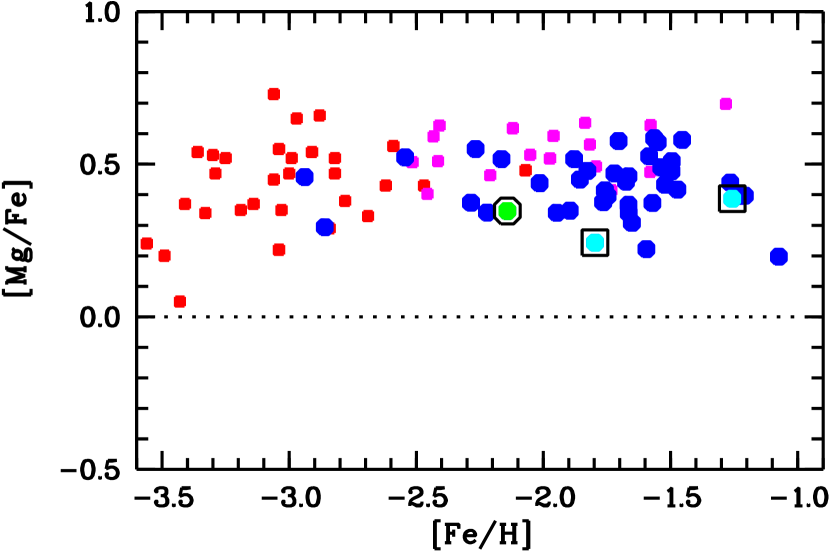
Figure 5: [Mg/Fe] versus [Fe/H] for the observed sample (blue circles). The young star is shown as a green dot inside a black circle, and the PISN candidates are shown as light-blue dots inside black squares. The comparison samples are the more metal-poor FS sample from (Cayrel et al., 2004a, red squares) and the sample of similar metallicity from Caffau et al. (2023, violet squares).

Titanium was derived from Ti ii lines for all stars in the sample, while for all but one star (RVS725), we could derive A(Ti) from Ti i lines. In the stellar parameter of the stars we investigated, Ti ii lines have small NLTE corrections, while the NLTE corrections for Ti i lines are non-negligible (see Sitnova et al., 2016, 2020). It was thus safer if we relied on Ti ii lines for the Ti abundance.

We investigated the light elements (Na, Al). For Na we investigated the lines at 568.8, 589.0, 589.6, 616.0, 818.3, and 819.4 nm, and we derived A(Na) for 38 stars in the sample. We looked in the material provided by Takeda et al. (2003) to derive NLTE corrections. For the sample, we obtained $\rm\langle[Na/Fe]\rangle=-0.13\pm 0.18$, with the lowest value being for RVS739 ($\rm[Na/Fe]=-0.57$, which becomes even lower when applying the NLTE correction on [Na/H]). To investigate the Al abundance, we used the resonance lines at 394 and 396 nm just for the star RVS738, while for the other stars we used weak lines where the NLTE correction is not expected to be large (see e.g. Baumueller & Gehren, 1997). The star RVS738 has $\rm[Al/Fe]=-1.07$ based on three lines and a line-to-line scatter below 0.02 dex.

The single K i line at 769.8 nm that we investigated to derive K abundances is contaminated by telluric absorption in the case of stars with large negative radial velocities. We thus decided to investigate this line through line profile fitting. The other reason supporting this choice was that the NLTE correction is large for this line in the stellar parameter range of the stars investigated here (Reggiani et al., 2019). An investigation with MyGIsFOS fit the line with a model more metal rich by more than 0.5 dex. We derived the K abundance for 31 stars in the sample. We derived the NLTE corrections in Reggiani et al. (2019), sometimes extrapolating in the tables provided. The large [K/Fe] ratios ($\rm\langle[K/Fe]\rangle=+0.58\pm 0.17$) are due to large NLTE effects, but once they were taken into account in [K/Fe], we obtained $\rm\langle[K/Fe]\rangle=+0.11\pm 0.14$.

In 41 stars of the sample, Mn was detected, and we found that all the stars have negative [Mn/Fe] ratios ($\rm\langle[Mn/Fe]\rangle=-0.28\pm 0.11$). This is due to NLTE effects on the Mn i lines (see e.g. Bergemann & Gehren, 2008; Bergemann et al., 2019). We investigated the NLTE effects in Bergemann et al. (2019) and applied them to the lines we used, and we found corrections to always be positive, from about 0.1 to 0.43 dex. For all but one star, we could derive the Ni abundance, which is in excellent agreement with Fe (for the 42 stars $\rm\langle[Ni/Fe]\rangle=-0.02\pm 0.05$).

We derived the Cu abundance for 21 stars in the sample, and they all have a negative [Cu/Fe] ratio ($\rm[Cu/Fe]=-0.52\pm 0.14$). Caffau et al. (2023) investigated the NLTE effects on Cu for a sample of stars of similar parameters and derived an NLTE correction on average slightly below +0.2 dex, so when applying these NLTE corrections, the stars in our sample would still keep a negative[Cu/Fe] ratio.

For 37 stars in the sample, Zn could be derived by investigating the Zn i lines at 472.2 and 481.0 nm (see Fig. 6). The NLTE corrections derived by interpolating in the values provided by Sitnova et al. (2022) are non-negative and small (not larger than 0.06 dex). When both lines are detected, the abundances derived from the two lines are generally in reasonable agreement. Just for one star (RVS734), the two lines provide abundances at almost 0.5 dex difference, but the S/N in this case is low (S/N=16 per pixel). Three stars in the sample (RVS709, RVS714, and RVS727) show a $\rm[Zn/Fe]<-0.3$. The star RVS709 is also poor in Cu ($\rm[Cu/Fe]=-0.82$; the lowest value in the sample), while the other two stars do not have any Cu detected. These three stars are good candidates as pair-instability supernova (PISN) descendants (see Salvadori et al., 2019; Caffau et al., 2023; Aguado et al., 2023a). The low Zn abundance could also point to the fact that these stars were accreted from a galaxy of such small mass to have allowed for a low enough star formation rate that the birth of massive stars was inhibited (see Mucciarelli et al., 2021).

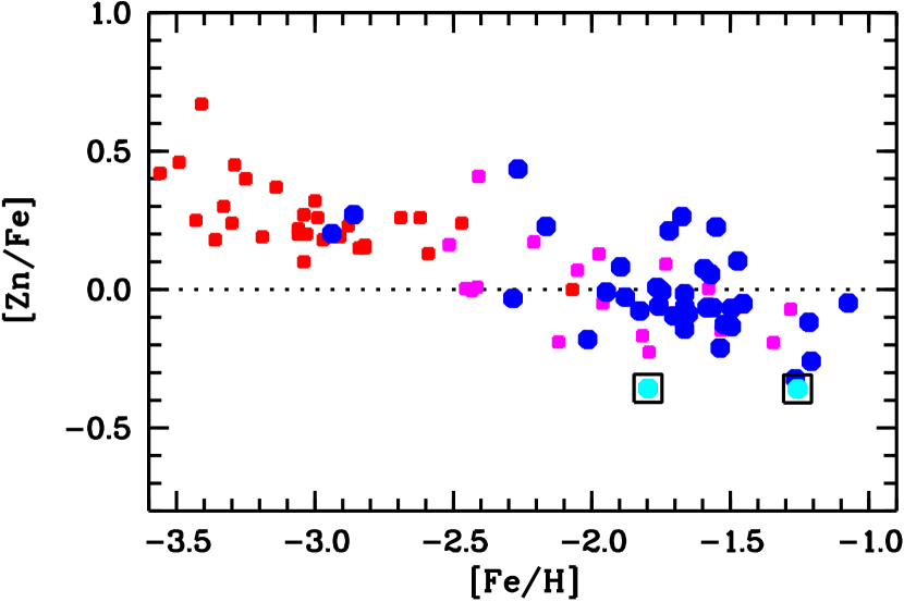
Figure 6: [Zn/Fe] versus [Fe/H] for the observed sample. Symbols are as in Fig. 5.

We derived the barium abundances by using line profile fitting. We used three Ba ii lines: 585 nm, 614 nm, and 649 nm. For the three lines, as recommended by Heiter et al. (2021), we used the oscillator strengths of Davidson et al. (1992). Following Korotin et al. (2015), we adopted hyperfine splitting only for the 649 nm line, and we adopted that in Heiter et al. (2021). For all three lines, we interpolated the NLTE corrections in the table of Korotin et al. (2015). We were able to derive the barium abundance for 42 stars. We investigated Europium through line profile fitting of the Eu ii line at 381.9, 412.9, 664.5, and 742.6 nm. For 35 stars in the sample, we were able to derive A(Eu). The [Eu/Fe] ratio (with Fe from Fe ii lines) is always positive with $\rm\langle[Eu/Fe]\rangle=0.65\pm 0.21$.

We decided to use the two stars with differences in radial velocity from the two spectra in order to check the precision of this set of data and separately analyse the two spectra. For RVS712, the average difference in the abundances we obtained from the two spectra is close to zero ($0.02\pm 0.06$ dex), with the differences in the range $[-0.1,0.1]$ dex. Also for RVS736, the average difference we obtained by analysing the two spectra is close to zero ($0.02\pm 0.08$ dex), with the differences in the range $[-0.1,0.15]$ dex. For Zn, whose abundance is based on the Zn i line at 481.0 nm, both spectra have an S/N around 15. We concluded that the precision of the chemical investigation is between 0.1 and 0.2 dex, according to the S/N of the spectra, which are summarised in Table 2.

4.3 Comparison with the RVS spectra

We retrieved from the Gaia archive the RVS spectra for two stars in our sample: RVS719 and RVS733. There are no astrophysical parameters for these two stars in Gaia DR3. Both spectra have an S/N per pixel between 20 and 30 at 855 nm, which are low for middle-resolution infra-red spectra. We analysed the RVS spectra to derive Fe and Ti abundances.

For RVS719, from four Fe i lines, we derived $\rm[Fe/H]=-1.26\pm 0.17$, to be compared to $\rm[Fe/H]=-1.21\pm 0.22$ from the complete UVES spectrum. From one single Ti i line, we derived $\rm[Ti/H]=-0.63$, to be compared to $\rm[Ti/H]=-0.70\pm 0.12$ from 25 lines from the UVES spectrum. The Ti i line investigated in the RVS spectrum was rejected in the UVES analysis because it is too strong, but it would provide [Ti/H]=-0.66.

For RVS733, we could only derive $\rm[Fe/H]=-1.32\pm 0.45$ from four Fe i lines, to be compared to $\rm[Fe/H]=-1.67\pm 0.19$ derived from the complete UVES spectrum. The agreement is well within the uncertainties.

5 Discussion

Three stars in the sample (RVS708, RVS709, RVS740) seem lower than the others in [Mg/Fe] and [Ca/Fe], while RVS726 has a low [Ca/Fe] but no Mg detection, and RVS745 has low [Mg/Fe] and [Ca/Fe] ratios, but this is consistent with other stars. This conjunction of low $\alpha$ elements and low [Zn/Fe] and [Cu/Fe] ratios makes RVS709 a perfect candidate as a PISN descendant. Salvadori et al. (2019) investigated from a theoretical point of view the chemical characteristics expected in a PISN descendant and highlighted that the effect is most evident at the metal-poor regime (with the most evident effect at $\rm-2\lesssim[Fe/H]\lesssim-1$) and overall on nitrogen, copper, and zinc. Since Cu and Zn abundance determinations are rare among chemical investigations in metal-poor stars, Aguado et al. (2023a) built a way to use all the abundances to select stars that can be PISN descendants and eventually observe them to derive A(Cu), A(Zn), and possibly also A(N). Recently, Xing et al. (2023) discovered another PISN descendant in the Galaxy. In Fig. 7, the [X/Fe] ratios (derived from neutral species) are compared for a Zn-poor star (RVS709), a Zn-normal star (RVS728), and a Zn-rich star (RVS740). The star RVS709 shows a systematic [X/Fe] ratio that is lower with respect to the other two stars. In Fig. 7, we also show the theoretical yields of Heger & Woosley (2002) for three masses, 168, 195, and 242 $M_{\odot}$, that end their lives as PISNs. It is clear from this comparison that none of these stars may have been formed from pure PISN ejecta. If PISN ejecta are diluted with gas polluted by less massive supernovae (SNe), then patterns like that of RVS709 can be reproduced (see Aguado et al., 2023b, for an extensive discussion).

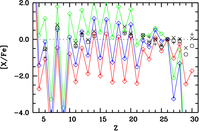
Figure 7: [X/Fe] for abundances derived from neutral lines for a Zn-poor (RVS709, open circles), a Zn-normal (RVS728, cross symbols), and a Zn-rich (RVS740, plus symbols) star. We also show the theoretical yields of Heger & Woosley (2002) for stellar masses of 168 $M_{\odot}$ (green lozenges and line), 195 $M_{\odot}$ (blue lozenges and line), and 242 $M_{\odot}$ (red lozenges and line).

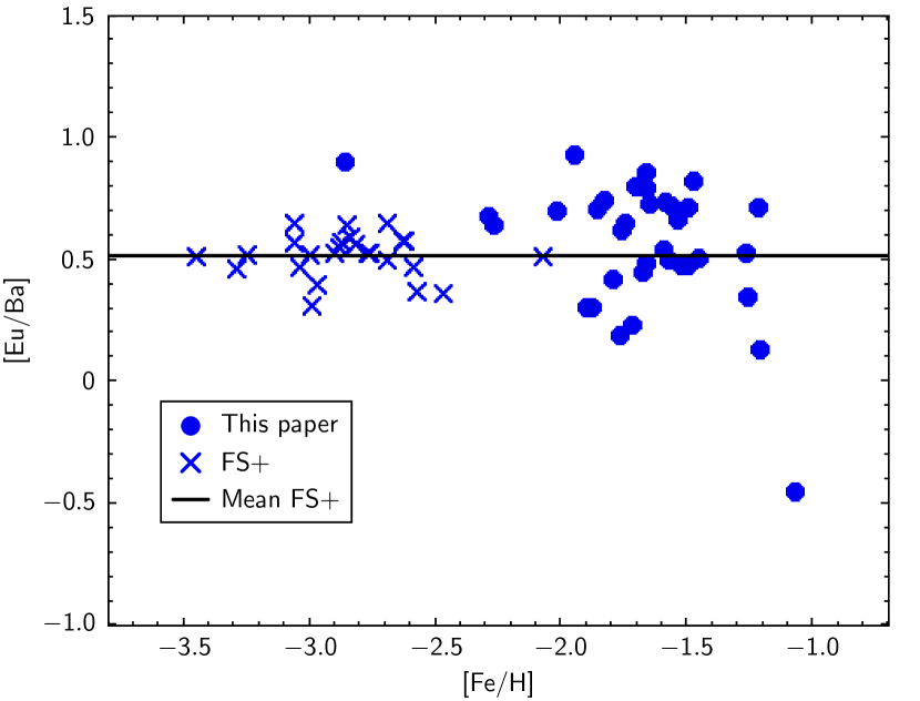
Figure 8: [Eu/Ba] versus [Fe/H] diagram. For our stars, the NLTE corrections to Ba have been applied. For comparison, we added stars from the First Stars sample (see text), labelled FS+. The solid horizontal line corresponds to the mean value of all the FS+ values.

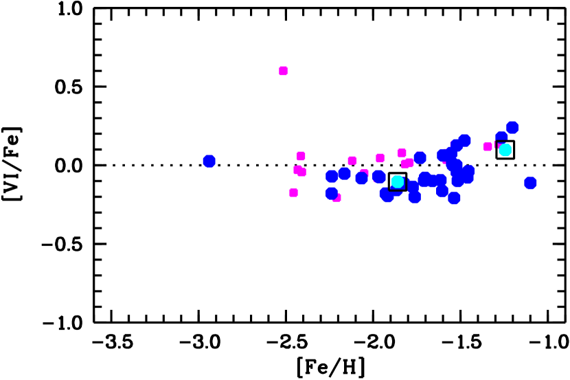
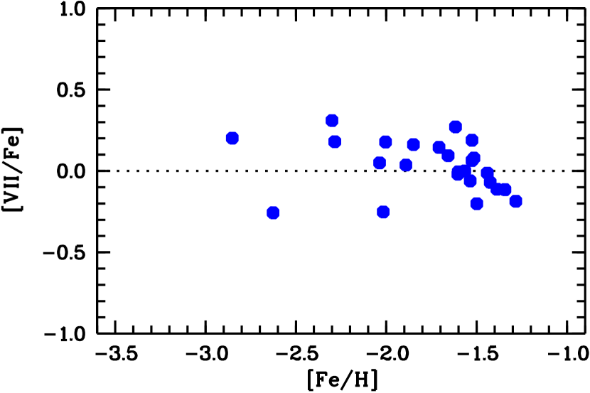
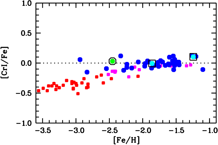
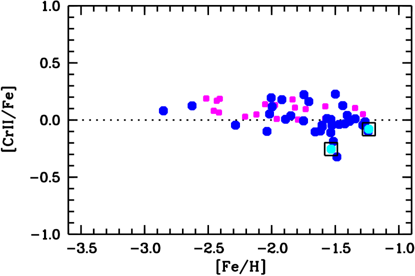
Figure 15: [X/Fe] versus [Fe/H] (for V and Cr). Symbols are as in Fig. 12. In [X/Fe] ratios for the ionised V and Cr, Fe is from Fe ii lines.

Europium is a pure $r-$process element, while barium is mainly an $s-$process element (Arlandini et al., 1999; Prantzos et al., 2020). The ratio Eu/Ba can be used as a diagnostic of the relative importance of the two processes in any stellar population. In Fig. 8, we show [Eu/Ba] as a function of [Fe/H] for our programme stars as well as for the First Stars sample (Cayrel et al., 2004b; François et al., 2007; Siqueira Mello et al., 2013), complemented with two measurements from Sneden et al. (2009) and Hill et al. (2017), labelled FS+ in the plot. The FS+ stars show a constant [Eu/Ba] ratio of 0.52 with a tiny scatter of 0.09 dex. This strongly suggests that both Eu and Ba are synthesised in the same process. This value is not far from the prediction of Wanajo (2007) of 0.62 for the hot $r-$process (see also Siqueira Mello et al., 2013, Fig. 15). Of the five stars with metallicities above –1.3, three have [Eu/Ba]$<0$. We tentatively interpreted this as a sign of Ba $s-$process production in AGB stars. For lower metallicity stars, however, the mean is very close to that of the FS+ sample, albeit with a larger scatter that is compatible with the lower S/N of our spectra with respect to those of the FS+ sample. This does suggest that in the most metal-poor part of the sample ($\rm[Fe/H]<-1.3$), both Eu and Ba are formed only by the $r-$process, and by inference, we may extend this hypothesis to all the neutron capture elements.

Caffau et al. (2020) and Bonifacio et al. (2024) investigated a sample of stars selected by their high speed with respect to the Sun. They required in Gaia DR2 a transverse velocity higher than 500 $\rm kms^{-1}$. The sample of stars we investigated was selected according to their high radial velocity in order to verify their reliability (discussed in Katz et al. in preparation). All of these stars (of this paper and the stars discussed in Bonifacio et al., 2024) are then expected to be halo stars. All of these selections collected mainly metal-poor stars, with a paucity of extremely metal-poor stars, and in the case of the stars analysed in this work, the most metal-poor star (RVS713) has $\rm[Fe/H]=-2.94$. It is true that extremely metal-poor stars ($\rm[Fe/H]<-3$) are rare objects, but the samples containing the stars we investigated are quite large (about 400 stars), and just a handful of stars (in Bonifacio et al., 2024) have $\rm[Fe/H]<-3$.

Another similarity with the investigations of Caffau et al. (2020) and Bonifacio et al. (2024) is the presence of stars compatible with a young age. The two stars RVS725 and RVS726 seem to be younger than 1 Ga, and they both are expected to have large masses. As discussed in Bonifacio et al. (2024), these stars can be evolved blue stragglers that resulted from the merger of three stars (in the case of RVS725, perhaps even four). The formation of a blue straggler by the merging of three stars is described by Meyer & Meyer-Hofmeister (1980), but as stated by Fiorentino et al. (2014), massive blue stragglers are very rare objects. To further support the small probability of forming a massive blue straggler from a triple system, one can first consider the low fraction of triple systems among solar-type stars ($9\%\pm 2\%$, Raghavan et al. 2010) and the low probability that in a destabilised triple system, a collision involving all three stars takes place (0.6%, Toonen et al., 2022). On the other hand, collisions involving only the inner pair are relatively common, up to 24% (Toonen et al., 2022). But these latter numbers are only for a destabilised triple system, which are only a fraction of all triple systems. These considerations explain why blue stragglers with masses larger than twice the turn-off mass are rare. Thus, the possibility must be confronted that these stars are really young, formed in a recent accretion event at the moment of the infall of the accreted object (a dwarf galaxy or a cluster) in the Milky Way. If so, the age of these stars would provide us with the time of the accretion events.

The 43 stars we chemically investigated are all metal-poor ($\rm[Fe/H]<-1$), but none is a CEMP star. This is surprising, as one would expect 21% of the stars to be CEMPs at the very metal-poor regime, $\rm[Fe/H]<-2$ (Lucatello et al., 2006). Clearly the numbers are small, but one would expect to see at least one star rich in carbon.

6 Conclusion

The chemical analysis of our sample of stars shows, by and large, the typical patterns found in other samples of metal-poor stars. What stands out is (i) there are up to three candidate PISN descendants with low $\alpha$ elements, Cu and Zn, and (ii) two are apparently young stars that can hardly be interpreted as blue stragglers without invoking the merging of multiple systems.

We confirm the small number of extremely metal-poor stars among samples of high-velocity stars. We point out that RVS721 lies within $10^{\prime\prime}$ of the track of the Gjoll stream (Ibata et al., 2019) associated with the globular cluster NGC 3201. The metallicity of the star is $-1.66\pm 0.16$ dex, which is a good match with the catalogue metallicity of the cluster, $-1.59$ dex (Harris, 1996), thus supporting the association.

Appendix A Variable stars

Figure 9: Lomb-Scargle periodogram of the $G$ epoch photometry of RVS711. The dotted line shows the level of false alarm probability $1.^{-4}$

Four stars are classified by Gaia DR3 as variables. The stars RVS708, RVS719 and RVS724 are classified as long period variables, with probabilities of over 70%, while RVS711 is classified as an RS Canum Venaticorum (RS CVn) variable, with a probability of 44%. No periods or other information beyond the epoch photometry is available from Gaia DR3.

A.1 RVS711

In our spectrum, the CaII H and K lines show a clear emission core, supporting the classification as an RS CVn. We computed the Lomb-Scargle periodogram using the $G$ data (see Fig. 9), and the only significative peak is evident at 120.48 days, which is quite high for an RS CVn, since most of these stars have periods below 20 days (Martínez et al. 2022). We tried to phase the data with this period and were unable to obtain a smooth light curve. It is probable that the timeseries is too short and sparsely sampled to provide an accurate period. Under these conditions, it is impossible to understand in which phase our spectrum was observed. However, the whole light curve spans a range of 0.05 mag in $G_{BP}-G_{RP}$, corresponding to less than 100 K. This is an additional error to be considered on our adopted effective temperature.

A.2 RVS708

This star has been classified as a long period variable by Heinze et al. (2018), named as ATO J283.9396-17.3013, as well as by Gaia DR3. Heinze et al. (2018) provided a period of 315.971905 days from a Lomb-Scargle periodogram. We tried to phase the Gaia $G$ epoch photometry (24 points) with this period but failed to obtain a smooth light curve. The $G_{BP}-G_{RP}$ colour spans a range of 0.07 mag in the Gaia DR3 epoch photometry. This corresponds to about 150 K and has to be considered an additional error on our adopted effective temperature. Our spectrum shows clear emissions in the Ca ii H and K lines.

A.3 RVS719

For this star, there is no information in the literature. We computed the Lomb-Scargle periodogram for the $G$ epoch photometry but could not identify any statistically significant peak. The $G_{BP}-G_{RP}$ colour spans a range of about 0.09 mag, corresponding to almost 200 K. This is an additional uncertainty on our adopted effective temperature.

A.4 RVS724

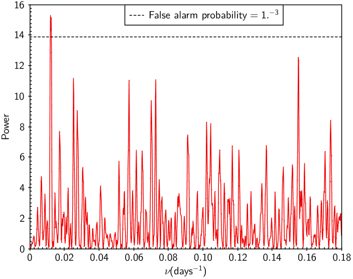
Figure 10: Lomb-Scargle periodogram of the $G$ epoch photometry of RVS724 The dotted line shows the level of false alarm probability $1.^{-3}$

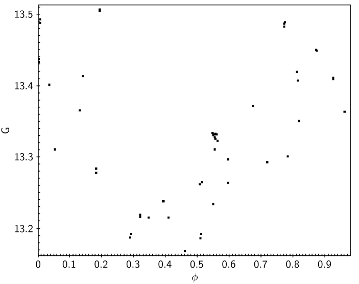
Figure 11: $G$ epoch photometry of RVS724 phased with a period of 84.45946 days.

We computed the Lomb-Scargle periodogram using the $G$ epoch photometry, and it is shown in Fig. 10. There is only one peak higher than the false alarm probability of $10^{-3}$, corresponding to a period of 84.45946 days. We phased the $G$ epoch photometry with this period, and the result is shown in Fig. 11. While the result is plausible, it is inconsistent with the precision of the Gaia photometry. This suggests that a longer timeseries is required to determine an accurate period, and we do not exclude that the star may be multi-periodic. This discourages us to use this curve to estimate the phase at which we observed the spectrum. In the epoch photometry, the $G_{BP}-G_{RP}$ colour spans a range slightly over 0.3 mag, which corresponds to over 600 K. This implies that the effective temperature that we derived from the mean colours is very uncertain. This is clear also from the two spectra at our disposal that provide different abundances, very likely because they were observed at different phases and different effective temperatures. Our spectra display a considerable level of activity with the presence of several emission lines.

Appendix B Details on some stars

Some of the stars have a sufficient S/N in the blue wavelength region to allow for an emission to be seen in the core of the Ca ii H and K lines, namely, RVS700, RVS701, RVS703, RVS704, RVS705, RVS707, RVS708, RVS711, RVS719, RVS724, and RVS736. In some stars, a P-cygni profile in $\rm H\alpha$ can be detected, including RVS701, RVS703, RVS704, RVS707, RVS708, RVS709, RVS719, RVS724, RVS726, RVS732, RVS733, RVS740, and RVS743. Some of the stars have already been investigated and are present in the literature.

B.1 RVS701

This star, as SMSS J120148.09-414126.6, has been investigated by Dietz et al. (2020), who derived $\rm[Fe/H]=-1.196$. This is to be compared to $\rm[Fe/H]=-1.584\pm 0.178$ from our analysis.

B.2 RVS705

According to Alksnis et al. (2001), this is a carbon star. The UVES spectrum confirms this finding.

B.3 RVS707

This star appears in the sample of Dietz et al. (2020), with $\rm[Fe/H]=-1.708$. This is in excellent agreement with our value of $\rm[Fe/H]=-1.758\pm 0.196$.

B.4 RVS728

This star is in the sample by Dietz et al. (2020), with $\rm[Fe/H]=-1.460$. This is close to our value of $\rm[Fe/H]=-1.571\pm 0.171$.

B.5 RVS733

Dietz et al. (2020) derived for this star $\rm[Fe/H]=-1.496$, while Hayes et al. (2018) adopted ($T\rm_{eff}$/$\log\,g$/[Fe/H]) of 4392/1.0647/–1.340, and Jönsson et al. (2020) adopted 4420/1.2902/–1.404. These values are to be compared to our values of 4336/1.49/$-1.675\pm 0.194$.

B.6 RVS743

According to Srinivasan et al. (2016), this is a red supergiant candidate of the Small Magellanic Cloud (SMC). According to the Gaia DR3 parallax ($0.03654\pm 0.01038$), the star is too close to belong to the SMC.

Appendix C Abundances

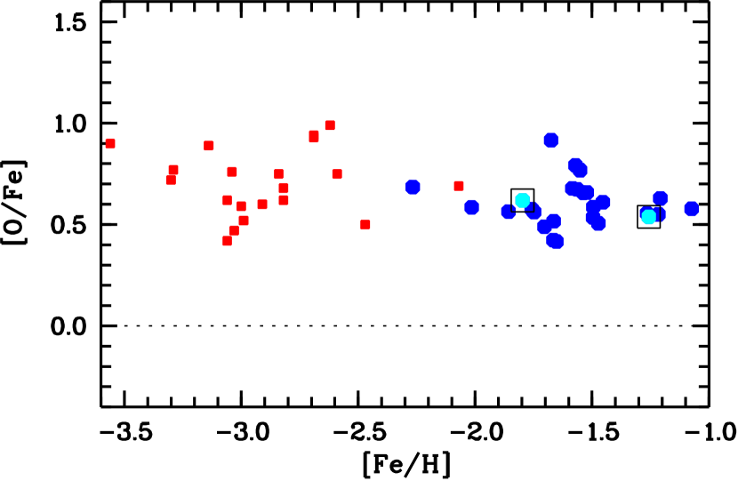
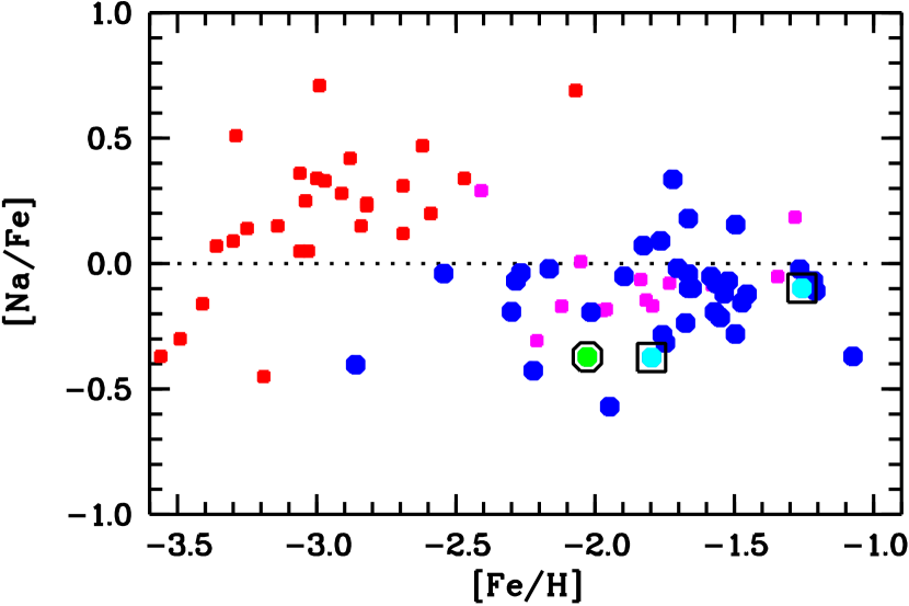
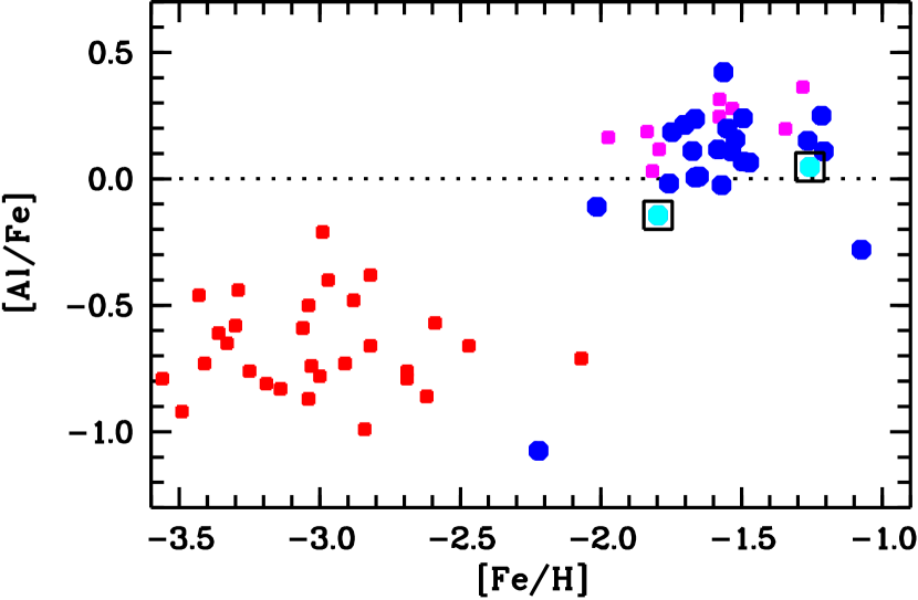
Figure 12: [X/Fe] versus [Fe/H] (for O, Na and Al) for the observed sample (blue circles). The young stars are shown as green dots inside black circles, and the PISN candidates are shown as light-blue dots inside black squares. The comparison samples are the more metal-poor FS sample from (Cayrel et al. 2004a, red squares) and the sample of similar metallicity from Caffau et al. (2023, violet squares).

The abundances are provided in an online table (Table C.1) available at CDS. The table contains the name of the star, the Gaia DR3 identifier, the stellar parameters, the abundances, and the NLTE corrections discussed in the text.

The lines used in the star-by-star analysis for all elements are provided at CDS in an online table (Table C.2). We recall that MyGIsFOS performed a fit in chosen wavelength ranges. In the table, all the lines of the designated elements presented in the range are reported. Except for the forbidden [OI] lines, we cut all the Fe i lines at $\rm\log{gf}<-3.5$, and for the other elements, we cut them at $\rm\log{gf}<-4.5$. We show the plots of [X/Fe] versus [Fe/H] for the abundances derived and provided in the online table compared to the sample from Cayrel et al. (2004a) and Caffau et al. (2023) for the elements not already shown in the main text.

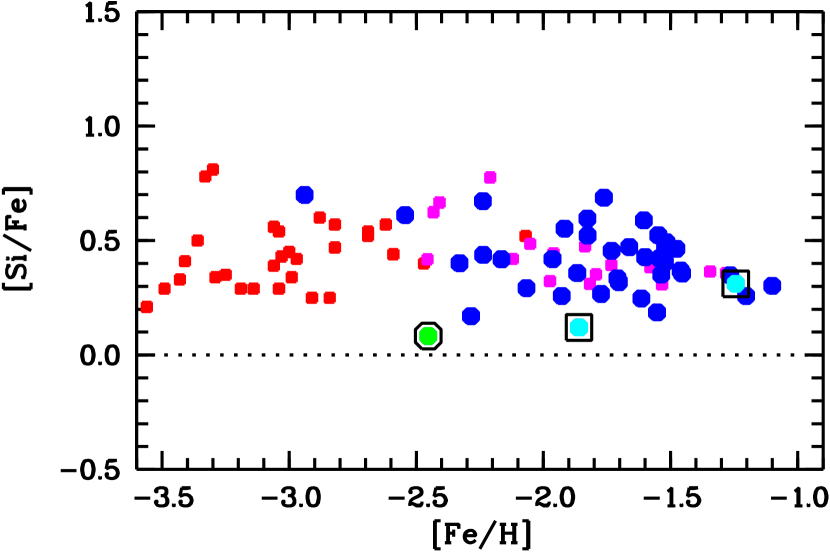
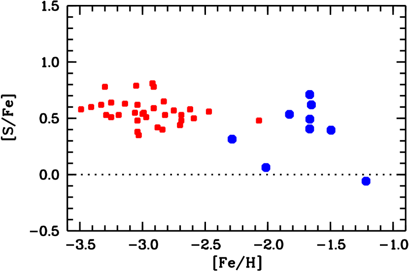
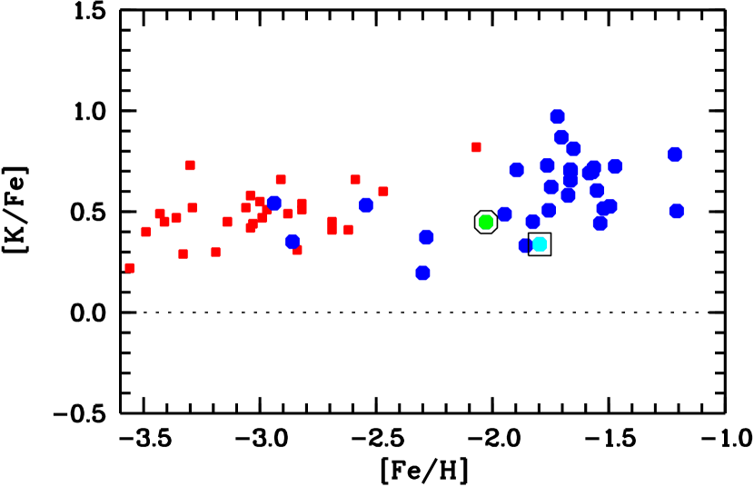
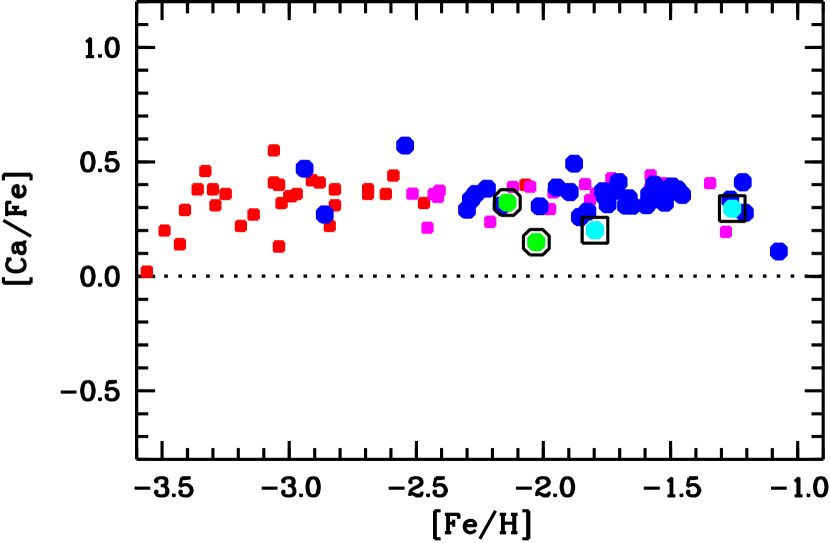
Figure 13: [X/Fe] versus [Fe/H] (for Si, S, K, and Ca) for the observed sample. Symbols and comparison samples are as in Fig. 12.

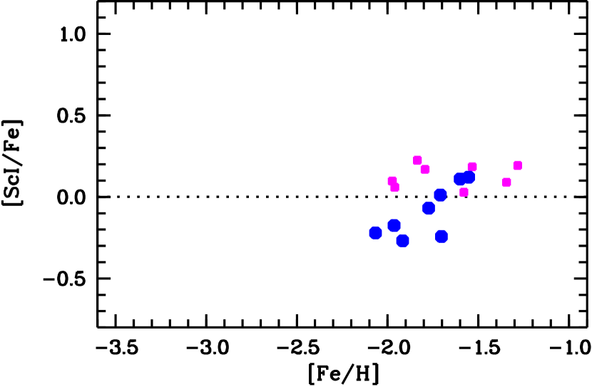
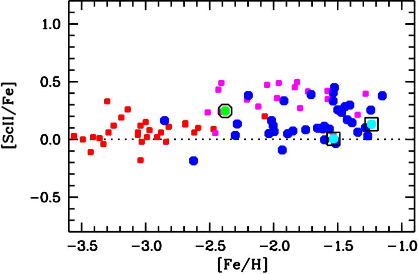
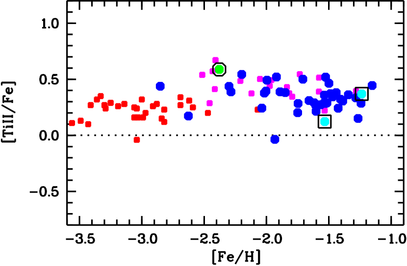
Figure 14: [X/Fe] versus [Fe/H] (for Sc and Ti). Symbols are as in Fig. 12. In [X/Fe] ratios for the ionised Sc and Ti, Fe is from Fe ii lines.

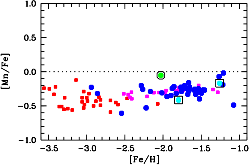
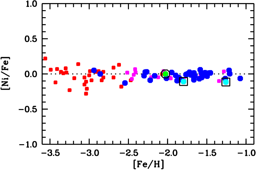
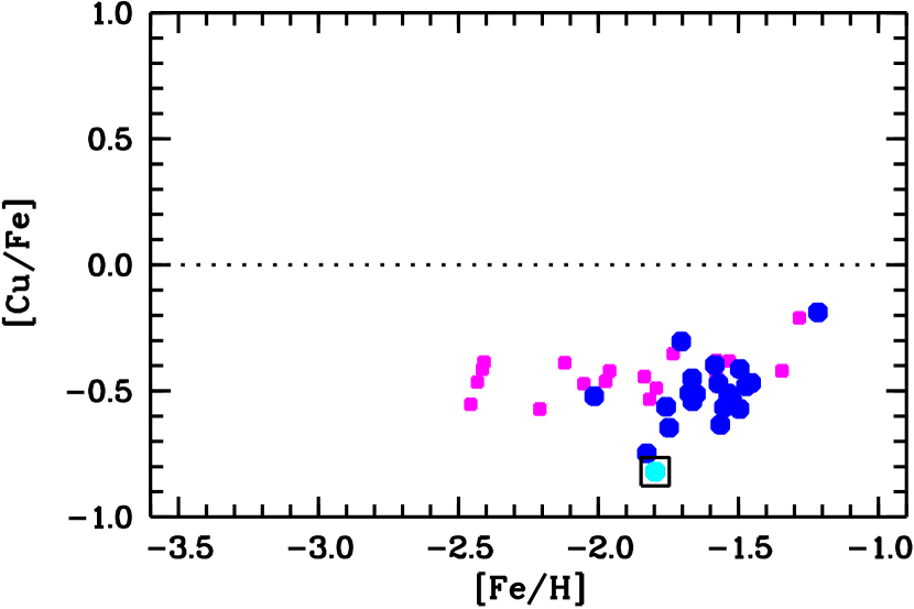
Figure 16: [X/Fe] versus [Fe/H] (for Mn, Ni, Cu and Co). Symbols are as in Fig. 12.

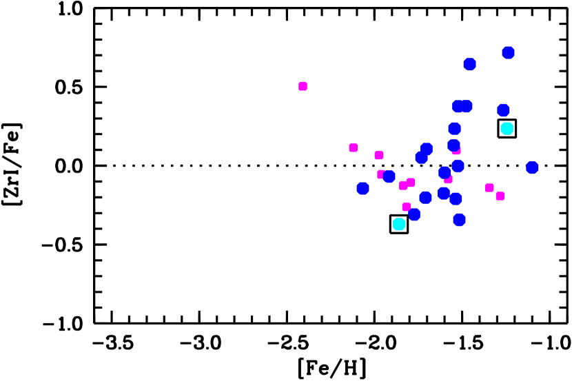
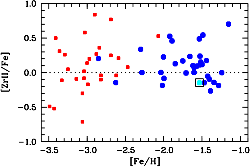
Figure 17: [X/Fe] versus [Fe/H] (for Y and Zr). Symbols are as in Fig. 12 except that here the FS sample is from François et al. (2007). In [X/Fe] ratios for the ionised Y and Zr, Fe is from Fe ii lines.