A classical density functional theory for solvation across length scales

Abstract

A central aim of multiscale modeling is to use results from the Schrödinger Equation to predict phenomenology on length scales that far exceed those of typical molecular correlations. In this work, we present a new approach rooted in classical density functional theory (cDFT) that allows us to accurately describe the solvation of apolar solutes across length scales. Our approach builds on the Lum, Chandler and Weeks (LCW) theory of hydrophobicity [J. Phys. Chem. B 103, 4570 (1999)] by constructing a free energy functional that uses a slowly-varying component of the density field as a reference. From a practical viewpoint, the theory we present is numerically simpler and generalizes to solutes with soft-core repulsion more easily than LCW theory. Furthermore, we also provide two important conceptual insights. First, the coarse-graining of the density field emerges naturally and justifies a coarse-graining length much smaller than the molecular diameter of water. Second, by assessing the local compressibility and its critical scaling behavior, we demonstrate that our LCW-style cDFT approach contains the physics of critical drying, which has been emphasized as an essential aspect of hydrophobicity by recent theories. As our theory is parameterized on the two-body direct correlation function of the uniform fluid and the liquid–vapor surface tension, it straightforwardly captures the temperature dependence of solvation. Moreover, we use our theory to describe solvation at a first-principles level, on length scales that vastly exceed what is accessible to molecular simulations.

Many of the most fundamental processes in nature, including protein folding, crystallization and self-assembly, occur in solution. Far from being an innocent bystander, the solvent often plays a vital role in determining the static and dynamic behaviors of these complex processes [1, 2, 3, 4], owing to the delicate balance of solute–solute, solute–solvent and solvent–solvent interactions. This provides a strong motivation to faithfully describe solvation behavior across a broad range of fields, from biological and chemical to physical and materials sciences. Solutes of interest can range in length scale from microscopic species [5] and nano-particles [6] to macromolecules [7] and extended surfaces [8]. Solvation is a multiscale problem.

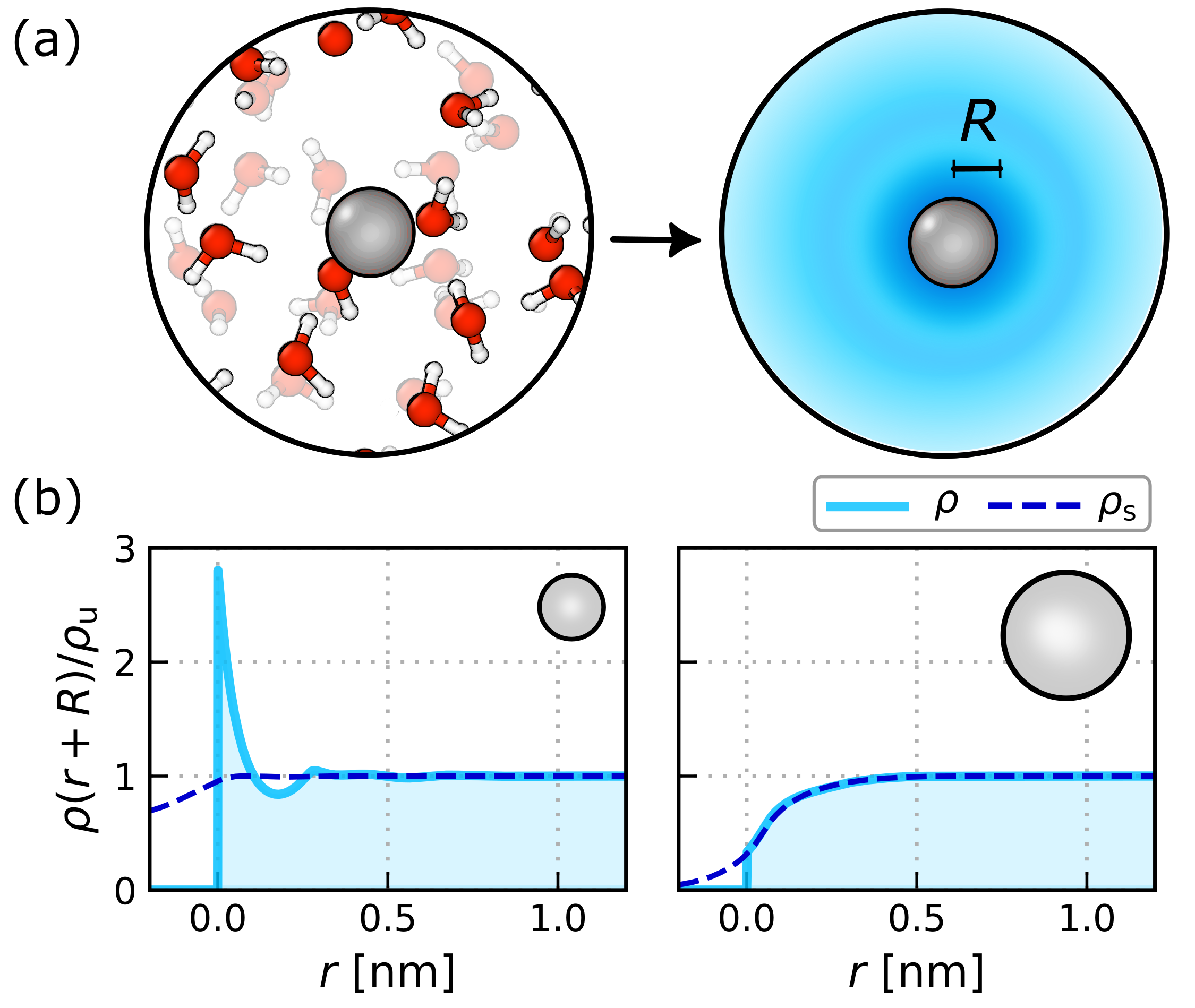
Figure 1: “Semi–implicit” solvation with cDFT. Our aim is to accurately describe aqueous solvation without explicitly sampling microscopic degrees of freedom, yet still retain information on essential correlations. This is shown schematically in (a). Such an approach should be able to predict, e.g., the average solvent density $\rho(r)$ around a solute, as depicted in (b). The solid blue lines represent $\rho(r+R)/\rho_{\rm u}$ for hard-sphere solutes of radius $R=0.3$ nm (left) and $R=3$ nm (right), where $\rho_{\rm u}$ is the uniform density of the bulk fluid. The cDFT that we derive relies upon finding an appropriate slowly-varying density $\rho_{\rm s}$ that can act as a suitable reference system.

The solvent, of course, comprises individual molecules. Molecular simulations therefore provide a natural approach to describe solvation, and bestow fine details at time and length scales that can be challenging to access with experimental approaches alone. Depending upon the approximations made in describing the intermolecular interactions, molecular simulations provide one of the most accurate means to estimate solvation free energies. Yet the relatively high computational cost associated with molecular simulations makes their routine use for solutes much larger than small organic compounds cumbersome and inefficient [9].

Implicit solvation models alleviate the computational burden by describing the solvent degrees of freedom as a structureless continuum [10, 11, 12, 13]. Such approaches are numerically efficient, making it possible to routinely handle large macromolecules in solution. The major drawback of implicit solvation models, however, is their failure to account for essential solvent correlations that may hold a prominent role in the process under investigation (see, e.g., Ref. 2). They also often make assumptions concerning the validity of macroscopic laws applied to the microscopic domain, which can lead to inconsistent results [14]. For these reasons, approaches that provide a coarse-grained description of solvation, while retaining information about essential molecular correlations, become very appealing. Such approaches should, for example, capture changes in the average equilibrium density field upon changing the solute–solvent interaction, as depicted in Fig. 1, without resorting to explicitly averaging microscopic degrees of freedom.

Motivated by both the seminal work of Lum, Chandler and Weeks (LCW) [15], and more recent developments in molecular density functional theory (mDFT) [16, 17, 18, 19, 20], in this article we present a classical density functional theory (cDFT) [21, 22, 23] for the solvation of apolar solutes. Although our approach differs from the original LCW theory, it retains the essential feature of appropriately accounting for both slowly- and rapidly-varying components of the density field, as shown in Fig. 1(b). From a practical viewpoint, the theory we present lends itself more readily to numerical evaluation than LCW theory, including application to solutes with soft repulsive cores and attractive tails. But as we will discuss, our approach also offers conceptual advantages.

The central quantity in any cDFT approach is the grand potential functional,

$$\varOmega_{\phi}[\rho]=\mathcal{F}_{\mathrm{intr}}[\rho]-\mu\int\!\!\mathrm{d}\bm{r}\,\rho(\bm{r})+\int\!\!\mathrm{d}\bm{r}\,\rho(\bm{r})\phi(\bm{r}),$$ (1)

where $\rho(\bm{r})$ is the average of a microscopic density field of the fluid, whose chemical potential is $\mu$. In the context of solvation, solute–solvent interactions are prescribed by the external potential $\phi(\bm{r})$. The intrinsic Helmholtz free energy functional, $\mathcal{F}_{\rm intr}$ does not depend on $\phi$. The equilibrium density is that which minimizes $\varOmega_{\phi}$.

While cDFT is in principle an exact theory, in general, approximations for $\mathcal{F}_{\rm intr}$ are required. For hard sphere systems, functionals based on Rosenfeld’s fundamental measure theory have proven highly successful [24, 25, 26]. Moreover, in cases where hard spheres act as a suitable reference fluid, attractive interactions can be reasonably treated in a mean-field fashion [22]. While approaches based on fundamental measure theory may capture some of the essential physics of more complex liquids such as water, it is unreasonable to expect quantitative agreement. Instead, in such cases, the mDFT approach [16, 17, 18, 19, 20] has shown great promise. The essential idea behind mDFT is that one can use the two-body direct correlation function,

$$c_{\rm u}^{(2)}(|\bm{r}-\bm{r}^{\prime}|)=-\beta\frac{\delta^{2}\mathcal{F}^{(\rm ex)}_{\rm intr}}{\delta\rho(\bm{r})\delta\rho(\bm{r^{\prime}})}\Bigg{|}_{\rho_{\rm u}},$$ (2)

obtained from simulations of the bulk fluid of uniform density $\rho_{\rm u}$ to parameterize the grand potential functional

$$\begin{split}\varOmega_{\phi}[\rho]=&\varOmega_{0}[\rho_{\rm u}]+\int\!\mathrm{d}\bm{r}\,\rho(\bm{r})\phi(\bm{r})+\Delta_{\rm u}\mathcal{F}_{\rm intr}^{\rm(id)}[\rho]\\ &-\frac{k_{\rm B}T}{2}\int\!\mathrm{d}\bm{r}\!\int\!\mathrm{d}\bm{r}^{\prime}\,\delta_{\rm u}\rho(\bm{r})\,c_{\rm u}^{(2)}(|\bm{r}-\bm{r}^{\prime}|)\,\delta_{\rm u}\rho(\bm{r}^{\prime})\\ &+\mathcal{F}_{\rm bridge}[\rho(\bm{r})].\end{split}$$ (3)

In Eq. 2, $\mathcal{F}^{(\rm ex)}_{\rm intr}$ is the excess contribution to $\mathcal{F}_{\rm intr}$. In Eq. 3, $\Delta_{\rm u}\mathcal{F}_{\rm intr}^{\rm(id)}$ is the change in the ideal contribution to $\mathcal{F}_{\rm intr}$ between systems with uniform and non-uniform density fields, and $\delta_{\rm u}\rho(\bm{r})=\rho(\bm{r})-\rho_{\rm u}$. The “bridge” functional, $\mathcal{F}_{\rm bridge}$, accounts for contributions to the excess part of $\mathcal{F}_{\rm intr}$ beyond quadratic order in $\delta_{\rm u}\rho(\bm{r})$. The solvation free energy is simply

$$\varOmega_{\rm solv}[\rho(\bm{r})]=\varOmega_{\phi}[\rho(\bm{r})]-\varOmega_{0}[\rho_{\rm u}].$$ (4)

Neglecting $\mathcal{F}_{\rm bridge}$ amounts to the hypernetted-chain approximation (HNCA) of integral equation theories [27]. Furthermore, upon linearizing $\Delta_{\rm u}\mathcal{F}_{\rm intr}^{\rm(id)}$, mDFT within the HNCA is equivalent, up to a small correction factor, to Chandler’s Gaussian field theory for solvation [28]. Aside from being numerically tractable, the HNCA provides reasonable accuracy for small solutes. However, as we have emphasized, solvation is a multiscale problem. To see this, consider that the solute simply excludes solvent density within a radius $R$ of its center. Whereas within the HNCA, $\varOmega_{\rm solv}$ scales indefinitely with the solute’s volume, for large enough solutes we know from macroscopic theory that it scales with the solute’s surface area, i.e., $\varOmega_{\rm solv}\sim 4\pi\gamma R^{2}$ where $\gamma$ is the liquid–vapor surface tension. Many previous studies have shown that for water under ambient conditions, this “hydrophobic crossover” occurs at $R\approx 1$ nm [15, 29, 30, 31, 32].

The failure of the HNCA for large solutes arises because it cannot describe water’s proximity to its liquid–vapor coexistence at ambient conditions [33, 22]. A natural progression, then, is to attempt to encode the physics of coexistence through $\mathcal{F}_{\rm bridge}$, while maintaining reference to the homogeneous fluid with density $\rho_{\rm u}$. Such an approach has been used with some success within the mDFT framework for simple point charge water models [20, 34]. However, as we show in the S.I., existing bridge functionals of this kind are generally not robust to the choice of water model. In this article, we will instead follow more closely the key idea underlying LCW theory: the fluid’s density can be separated into a slowly-varying component that can sustain interfaces and liquid–vapor coexistence, and a rapidly-varying component that describes the local structure on microscopic length scales [15, 35].

In the following, we will describe how these ideas from LCW theory can be used to develop a cDFT approach to solvation of apolar solutes across both small and large length scales. We will validate our theory against available simulation data for the solvation of both hard- and soft-core solutes. We will show that the physics of critical drying, which is essential for a faithful description of solvophobicity on large length scales, is well-described. We will also demonstrate that our approach captures a distinguishing feature of solvophobicity in complex liquids such as water— the “entropic crossover”—that is absent in simple liquids. We will use our theory to describe the hydrophobic effect at an ab initio level, on length scales inaccessible to molecular simulations.

A cDFT built on separation of length scales

In this section, we will provide an overview of the most salient aspects of the theory; a complete derivation is presented in the S.I.

The essential idea underlying our approach is formally similar to that of the HNCA. However, instead of choosing a fluid of uniform density, we suppose that there exists some inhomogeneous, but slowly-varying, density field $\rho_{\rm s}(\bm{r})$ that acts as a suitable reference. Expanding around $\rho_{\rm s}$,

$$\begin{split}\mathcal{F}^{(\rm ex)}_{\rm intr}[\rho]&=\;\mathcal{F}^{(\rm ex)}_{\rm s,intr}[\rho_{\rm s}]-k_{\rm B}T\int\!\mathrm{d}\bm{r}\,c_{\rm s}^{(1)}(\bm{r})\delta_{\rm s}\rho(\bm{r})\\ &-\frac{k_{\rm B}T}{2}\int\!\mathrm{d}\bm{r}\!\int\!\mathrm{d}\bm{r}^{\prime}\,\delta_{\rm s}\rho(\bm{r})c_{\rm s}^{(2)}(\bm{r},\bm{r}^{\prime})\delta_{\rm s}\rho(\bm{r}^{\prime})+\ldots,\end{split}$$ (5)

where $\mathcal{F}^{(\rm ex)}_{\rm s,intr}$ is the intrinsic excess Helmholtz free energy of the reference system, and $\delta_{\rm s}\rho(\bm{r})=\rho(\bm{r})-\rho_{\rm s}(\bm{r})$. The one- and two-body direct correlation functions are obtained from functional derivatives of $\mathcal{F}^{(\rm ex)}_{\rm s,intr}$. We anticipate that $\mathcal{F}^{(\rm ex)}_{\rm s,intr}$ forms part of a known grand potential functional, $\varOmega_{\rm s}$, that reasonably describes the behavior of slowly varying densities. Moreover, we suppose that reasonable approximations exist for $c^{(2)}_{\rm s}(\bm{r},\bm{r}^{\prime})$. Supposing $\rho_{\rm s}$ were known, we would simply add Eq. 5 to $\mathcal{F}^{(\rm id)}_{\rm s,intr}$, substitute into Eq. 1, resulting in a slightly modified version of Eq. 3. But in general, we do not know $\rho_{\rm s}(\bm{r})$. The approach of LCW is to introduce an additional “unbalancing potential” to $\varOmega_{\rm s}$ that accounts for the extra unbalanced attractive energy density arising from the rapidly varying $\rho(\bm{r})$. Our aim is to derive a similar coupling within the cDFT framework. To this end, we can expand $\mathcal{F}^{(\rm ex)}_{\rm s,intr}$ around an auxiliary reference density $\rho_{\rm r}(\bm{r})$,

$$c_{\rm s}^{(1)}(\bm{r})=c_{\rm r}^{(1)}(\bm{r})+\int\!\mathrm{d}\bm{r}^{\prime}\,c_{\rm r}^{(2)}(\bm{r},\bm{r}^{\prime})\delta_{\rm r}\rho_{\rm s}(\bm{r}^{\prime}),$$ (6)

where, $c_{\rm r}^{(1)}$ and $c_{\rm r}^{(2)}$ are the one- and two-body direct correlation functions of the auxiliary system and $\delta_{\rm r}\rho_{\rm s}(\bm{r})=\rho_{\rm s}(\bm{r})-\rho_{\rm r}(\bm{r})$. We will not say much regarding $\rho_{\rm r}$, other than we choose it to be arbitrarily close to $\rho_{\rm s}$, to the extent that we will ultimately set $\rho_{\rm r}=\rho_{\rm s}$. In this sense, its role is similar to an auxiliary field typically introduced in field theories (see, e.g., Ref. 36 in the context of solvation). Substituting Eq. 6 into Eq. 5, we obtain

$$\begin{split}\mathcal{F}^{(\rm ex)}_{\rm intr}[\rho]=&\mathcal{F}^{(\rm ex)}_{\rm s,intr}[\rho_{\rm s}]-k_{\rm B}T\int\!\mathrm{d}\bm{r}\,c_{\rm r}^{(1)}(\bm{r})\delta_{\rm s}\rho(\bm{r})\\ &-\frac{k_{\rm B}T}{2}\int\!\mathrm{d}\bm{r}\!\int\!\mathrm{d}\bm{r}^{\prime}\,\delta_{\rm s}\rho(\bm{r})c_{\rm s}^{(2)}(\bm{r},\bm{r}^{\prime})\delta_{\rm s}\rho(\bm{r}^{\prime})\\ &-k_{\rm B}T\int\!\mathrm{d}\bm{r}\!\int\!\mathrm{d}\bm{r}^{\prime}\,\delta_{\rm s}\rho(\bm{r})c_{\rm r}^{(2)}(\bm{r},\bm{r}^{\prime})\delta_{\rm r}\rho_{\rm s}(\bm{r}^{\prime}).\end{split}$$ (7)

The final term in Eq. 7 acts to couple fluctuations in the full density with those of the slowly varying density. To identify its contributions that we will ultimately associate with $\varOmega_{\rm s}$, we assume that $c_{\rm r}^{(2)}$ can be split in a similar fashion, i.e.,

$$c_{\rm r}^{(2)}(\bm{r},\bm{r}^{\prime})=c_{{\rm r},0}^{(2)}(\bm{r},\bm{r}^{\prime})+c_{{\rm r},1}^{(2)}(\bm{r},\bm{r}^{\prime}),$$ (8)

where $c_{{\rm r},0}^{(2)}(\bm{r},\bm{r}^{\prime})\simeq 0$ for $|\bm{r}-\bm{r}^{\prime}|>\ell$, where $\ell$ is a molecular length scale. Conversely, $c^{(1)}_{{\rm r},1}$ is slowly varying over length scales comparable to $\ell$. Introducing the ideal contribution, and using the relationship between $c^{(1)}_{\rm r}(\bm{r})$ and $\mu$, we obtain

$$\begin{split}\varOmega_{\phi}[\rho]=&\varOmega_{\mathrm{s}}[\rho_{\mathrm{s}}]+\!\int\!\!\mathrm{d}\bm{r}\,\phi(\bm{r})\rho(\bm{r})\\ &+k_{\mathrm{B}}T\!\int\!\!\mathrm{d}\bm{r}\,\left[\rho(\bm{r})\ln\left(\frac{\rho(\bm{r})}{\rho_{\mathrm{r}}(\bm{r})}\right)-\rho(\bm{r})\right]\\ &-k_{\mathrm{B}}T\!\int\!\!\mathrm{d}\bm{r}\,\left[\rho_{\mathrm{s}}(\bm{r})\ln\left(\frac{\rho_{\mathrm{s}}(\bm{r})}{\rho_{\mathrm{r}}(\bm{r})}\right)-\rho_{\mathrm{s}}(\bm{r})\right]\\ &-\frac{k_{\mathrm{B}}T}{2}\!\int\!\!\mathrm{d}\bm{r}\!\!\int\!\!\mathrm{d}\bm{r}^{\prime}\,\delta_{\mathrm{s}}\rho(\bm{r})\,c^{(2)}_{\mathrm{s}}(\bm{r},\bm{r}^{\prime})\,\delta_{\mathrm{s}}\rho(\bm{r}^{\prime})\\ &-k_{\mathrm{B}}T\!\int\!\!\mathrm{d}\bm{r}\!\!\int\!\!\mathrm{d}\bm{r}^{\prime}\,\delta_{\mathrm{s}}\rho(\bm{r})\,c^{(2)}_{\mathrm{r},0}(\bm{r},\bm{r}^{\prime})\,\delta_{\mathrm{r}}\rho_{\mathrm{s}}(\bm{r}^{\prime}),\\ \end{split}$$ (9)

where

$$\begin{split}\varOmega_{\mathrm{s}}[\rho_{\mathrm{s}}]=&\mathcal{F}_{\mathrm{s,intr}}[\rho_{\mathrm{s}}]-\mu\!\int\!\!\mathrm{d}\bm{r}\rho_{\mathrm{s}}(\bm{r})\\ &-k_{\mathrm{B}}T\!\int\!\!\mathrm{d}\bm{r}\!\!\int\!\!\mathrm{d}\bm{r}^{\prime}\,\delta_{\mathrm{s}}\rho(\bm{r})\,c^{(2)}_{\mathrm{r},1}(\bm{r},\bm{r}^{\prime})\,\delta_{\mathrm{r}}\rho_{\mathrm{s}}(\bm{r}^{\prime}).\\ \end{split}$$ (10)

Note that $\varOmega_{\rm s}$ is a functional of $\rho_{\rm s}$; its dependence on $\rho(\bm{r})$ is parametric.

To find the equilibrium properties of the system, we need to minimize $\varOmega_{\phi}$ with respect to $\rho(\bm{r})$. For a given $\rho_{\rm s}(\bm{r})$, minimizing $\varOmega_{\phi}$ and setting $\rho_{\rm r}=\rho_{\rm s}$ gives

$$\rho(\bm{r})=\rho_{\rm s}(\bm{r})\exp\left[-\beta\phi(\bm{r})+\int\!\mathrm{d}\bm{r}^{\prime}\,c^{(2)}_{\rm s}(\bm{r},\bm{r}^{\prime})\delta_{\rm s}\rho(\bm{r}^{\prime})\right].$$ (11)

Of course, we need to find $\rho_{\rm s}(\bm{r})$. By definition, it is slowly-varying, i.e., it does not change significantly over length scales comparable to $\ell$. In such cases, it is reasonable to employ a square-gradient approximation,

$$\begin{split}\varOmega_{\rm s}[\rho_{\rm s}]&\approx\int\!\mathrm{d}\bm{r}\,\left[\omega(\rho_{\rm s})+\frac{m}{2}|\nabla\rho_{\rm s}(\bm{r})|^{2}\right]\\ &-k_{\mathrm{B}}T\!\int\!\!\mathrm{d}\bm{r}\!\!\int\!\!\mathrm{d}\bm{r}^{\prime}\,\delta_{\mathrm{s}}\rho(\bm{r})\,c^{(2)}_{\mathrm{r},1}(\bm{r},\bm{r}^{\prime})\,\delta_{\mathrm{r}}\rho_{\mathrm{s}}(\bm{r}^{\prime}),\\ \end{split}$$ (12)

where $\omega(\rho_{\rm s})$ is the local grand potential density. The coefficient of $|\nabla\rho_{\rm s}|^{2}$ is in principle a function of the slowly varying density, $m(\rho_{\rm s})$. As a simplifying approximation, in most of what follows we will treat $m$ as a constant independent of density; for spherical solutes, this yields the correct limiting behavior for both $R\to 0$ and $R\to\infty$. For $R$ in the crossover regime, we will show that the extra flexibility afforded by allowing $m$ to vary in a systematic, yet practical, way with $\rho_{\rm s}$ yields quantitative agreement for intermediate solute sizes. For a given $\rho(\bm{r})$, minimizing $\varOmega_{\rm s}$ with respect to $\rho_{\rm s}$ and setting $\rho_{\rm r}=\rho_{\rm s}$, we find,

$$\omega^{\prime}(\rho_{\rm s})-m\nabla^{2}\rho_{\rm s}(\bm{r})+\psi(\bm{r})=0,$$ (13)

where $\omega^{\prime}$ indicates partial differentiation with respect to $\rho_{\rm s}$, and

$$\psi(\bm{r})=-k_{\rm B}T\int\!\mathrm{d}\bm{r}^{\prime}\,c_{{\rm r},1}^{(2)}(\bm{r},\bm{r}^{\prime})[\rho(\bm{r})-\rho_{\rm s}(\bm{r}^{\prime})].$$ (14)

Equations 11 and 13 provide a set of coupled equations that need to be solved self-consistently, and bare a striking resemblance to LCW theory. Indeed, $\psi(\bm{r})$ plays the role of the unbalancing potential in Ref. 15. The formal similarity can be made more apparent if we introduce the coarse-graining procedure,

$$\overline{\rho}(\bm{r})=\frac{\int\!\mathrm{d}\bm{r}^{\prime}\,c^{(2)}_{{\rm r},1}(\bm{r},\bm{r}^{\prime})\rho(\bm{r}^{\prime})}{\int\!\mathrm{d}\bm{r}^{\prime}\,c^{(2)}_{{\rm r},1}(\bm{r},\bm{r}^{\prime})}.$$ (15)

Equation 13 then reads

$$\omega^{\prime}(\rho_{\rm s})=m\nabla^{2}\rho_{\rm s}(\bm{r})+2a(\bm{r})[\overline{\rho}(\bm{r})-\overline{\rho}_{\rm s}(\bm{r})],$$ (16)

with

$$2a(\bm{r})=k_{\rm B}T\int\!\mathrm{d}\bm{r}^{\prime}\,c^{(2)}_{{\rm r},1}(\bm{r},\bm{r}^{\prime}).$$ (17)

The coarse-graining procedure prescribed by Eq. 15 has emerged from our theory as a natural consequence of separating the density into its slowly- and rapidly-varying components. However, it is cumbersome to evaluate. Expressing $\psi$ in terms of the coarse-grained density fields (Eq. 16) therefore also serves a practical purpose, as we can estimate its value using an approximate coarse-grained density field

$$\overline{\rho}(\bm{r})\approx(2\pi\lambda^{2})^{-3/2}\int\!\mathrm{d}\bm{r}^{\prime}\,\exp(-|\bm{r}-\bm{r}^{\prime}|^{2}/2\lambda^{2})\rho(\bm{r}^{\prime}).$$ (18)

Along with the coarse-graining length $\lambda$, we now treat $a$ as a parameter that needs to be determined. As detailed in the S.I., we estimate their values by using a hard sphere reference fluid for which $c_{{\rm r},0}^{(2)}$ is known. For liquid water at 300 K and $\beta\delta\mu=\beta(\mu-\mu_{\rm coex})\approx 10^{-3}$, where $\mu_{\rm coex}$ is the chemical potential at coexistence (corresponding to $\rho_{\rm u}\approx 33.234\,\mathrm{nm}^{-3}$ for SPC/E water), we obtain an acceptable range of the coarse-graining parameters $a\approx 200$–$300$ kJ cm³ mol^-2 and $\lambda\approx 0.08$–$0.11$ nm. This range for $\lambda$ is comparable to the coarse-graining length derived in Ref. 32 for a lattice-based version of LCW theory that emphasizes the importance of capillary wave fluctuations.

For $\omega(\rho_{\rm s})$, we employ the following form

$$\omega(\rho_{\mathrm{s}})=\omega_{\mathrm{coex}}(\rho_{\mathrm{s}})-\rho_{\mathrm{s}}\delta\mu,$$ (19)

where $\delta\mu=\mu-\mu_{\mathrm{coex}}$, $\mu_{\mathrm{coex}}$ is the chemical potential at coexistence and $\omega_{\mathrm{coex}}$ takes a quartic form,

$$\omega_{\rm coex} (\rho_{\rm s})=\frac{C}{2}\left(\rho_{\mathrm{s}}-\rho_{\mathrm{l}}\right)^{2}\left(\rho_{\mathrm{s}}-\rho_{\mathrm{v}}\right)^{2}+$$

$$\frac{D}{4}\left(\rho_{\mathrm{s}}-\rho_{\mathrm{l}}\right)^{4}\left(\rho_{\mathrm{s}}-\rho_{\mathrm{v}}\right)^{4}h(\rho_{\rm s}-\rho_{\rm v})h(\rho_{\rm l}-\rho_{\rm s}),$$ (20)

with $\rho_{\mathrm{l}}$ and $\rho_{\mathrm{v}}$ the liquid and vapor densities at coexistence, and $h(\rho_{\rm s})$ the Heaviside step function. The curvature at the minima is determined by $C$, whose value we set to be consistent with the compressibility of the bulk fluid $\chi_{\rm u}$. Together, $D$ and $m$ determine $\gamma$ and the shape of the free liquid-vapor interface. Details of our parameterization procedure are provided in the S.I. For a practical theory, all that is left to establish is the two-body correlation function $c^{(2)}_{\rm s}(\bm{r},\bm{r}^{\prime})$. We adopt the following simple form

$$c^{(2)}_{\mathrm{s}}(\bm{r},\bm{r}^{\prime})\approx c^{(2)}_{\mathrm{u}}(|\bm{r}-\bm{r}^{\prime}|)\rho_{\mathrm{s}}(\bm{r})\rho_{\mathrm{s}}(\bm{r}^{\prime})\rho_{\mathrm{u}}^{-2},$$ (21)

which is exact in the limits of homogeneity and low density, and interpolates smoothly between these two regimes. While other reasonable approximations could be made for $c^{(2)}_{\mathrm{s}}(\bm{r},\bm{r}^{\prime})$, ours is in alignment with the one adopted by LCW theory for the susceptibility.

In this section, we have derived a cDFT for solvation that aims to describe both the short-wavelength perturbations induced by effects of excluded volume, and the physics of liquid–vapor coexistence relevant for larger solutes. We have also described approximations for the coarse-grained density and inhomogeneous two-body direct correlation function that facilitate numerical evaluation. While our theory is appropriate for arbitrarily complex forms of apolar solute–solvent interaction, for demonstrative purposes, we will focus on spherical solutes and planar walls. These simple geometries, however, are sufficient to make connections with existing theories and highlight the advantages of our approach.

Solvation of spherical solutes, both hard and soft

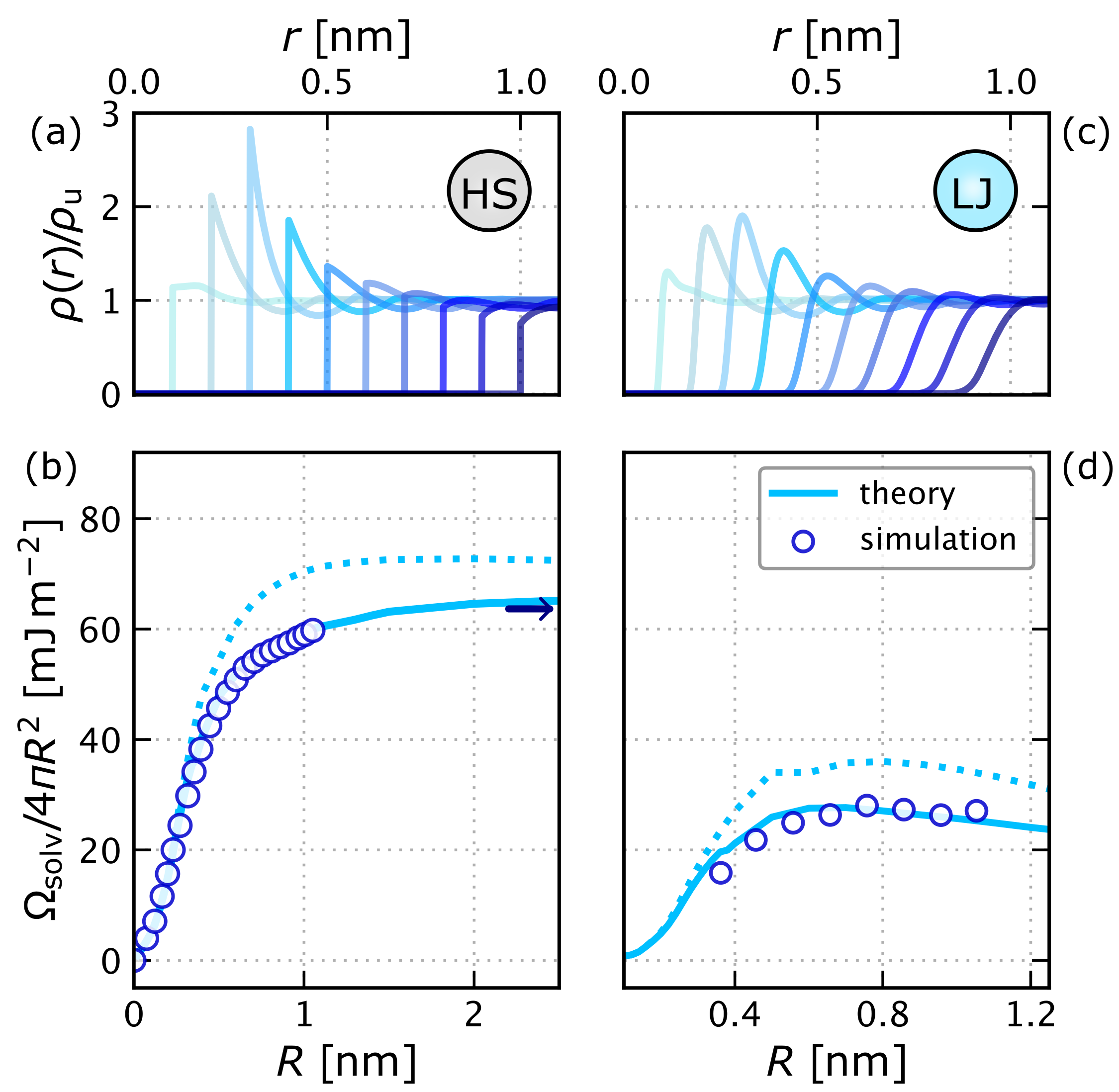
Figure 2: Solvation of spherical apolar solutes with cDFT. By solving Eqs. 11 and 16 self-consistently, we have obtained $\rho(r)$ and $\varOmega_{\rm solv}$, shown in (a) and (b) respectively, for hard-sphere solutes of different $R$ centered at the origin. When using $m(\rho_{\rm s}^{\ast})$ [(b), solid line], our theory is in quantitative agreement with results from molecular simulations [29]. If we take $m$ to be independent of density [(b), dotted line] we find qualitative agreement, but $\varOmega_{\rm solv}$ is overestimated for $R\gtrsim 0.5$ nm. In both cases, $\varOmega_{\rm solv}/4\pi R^{2}\sim\gamma=63.6\,\mathrm{mJ\,m^{-2}}$ (indicated by the blue arrow [37]), as $R\to\infty$. In (c) and (d) we show corresponding results for a LJ solute, and again we observe good agreement with molecular simulations [38]. Note that we have used the same parameterization as (a) and (b). All results from our theory have been obtained for SPC/E water ($T=300$ K, $\beta\delta\mu\approx 10^{-3}$, $a=200$ kJ cm³ mol^-2 and $\lambda=0.08$ nm).

We first consider the paradigmatic test case for any theory of hydrophobicity: the solvation of a hard-sphere solute in water under ambient conditions ($T=300\,\mathrm{K}$, $\beta\delta\mu\approx 10^{-3}$). To this end, in Figs. 2(a) and 2(b) we present $\rho(r)$ and $\varOmega_{\rm solv}$ obtained from self-consistent solution of Eqs. 11 and 16, parameterized for a simple point charge model of water (SPC/E [39]), as we increase the solute radius $R$. First treating $m$ as a constant (dotted line in Fig. 2), we see that our cDFT approach broadly captures the behavior observed in molecular simulations [29], with $\varOmega_{\rm solv}$ increasing with volume for small solutes, before crossing over to $\varOmega_{\rm solv}/4\pi R^{2}\sim\gamma$ for $R\gtrsim 1$ nm. Like previous treatments rooted in LCW theory, however, we also see that results from theory overestimate $\varOmega_{\rm solv}$ in the crossover regime.

Empirically, agreement with simulation results in the crossover regime could be attained by reducing the value of $m$. In the context of our theory, this implies that the optimal reference density for finite $R$ has a sharper interfacial thickness that the free liquid-vapor interface. Simply reducing $m$ in such a manner, however, would result in an incorrect limiting behavior as $R\to\infty$. But this observation motivates us to vary $m$, in a linear fashion, with a characteristic feature of the slowly-varying density $\rho^{\ast}_{\rm s}$. Specifically, $\rho^{\ast}_{\rm s}$ is the value where $\rho_{\rm s}=\rho$ for the first time as $R$ increases. Further details are provided in the S.I. As we see in Fig. 2(b) (solid line), with $m(\rho^{\ast}_{\rm s})$ our cDFT describes the simulation data quantitatively.

For hard spheres in water, the main advantage of our approach compared to LCW theory is primarily conceptual: $\varOmega_{\rm solv}$ follows directly from the minimization of $\varOmega_{\phi}$, as opposed to relying on, e.g., thermodynamic integration [40, 30, 41]. From a practical viewpoint, the cDFT approach is also numerically simpler to implement, as discussed in detail in Ref. 28. But its main advantages compared to LCW theory become apparent once we depart from the solvation of ideal hydrophobes. In LCW theory, it is assumed that the solute–solvent interaction can be separated into repulsive and attractive contributions, $\phi=\phi_{\mathrm{rep}}+\phi_{\mathrm{att}}$. While $\phi_{\mathrm{att}}$ can be accounted for straightforwardly in the slowly-varying part, $\phi_{\mathrm{rep}}$ must be approximated by a hard-core potential, and the solvent density is solved subject to the constraint $\rho(r)=0$ inside the solute [36]. For cDFT approaches such as ours, such an approximation is not needed. Instead, we simply minimize $\varOmega_{\phi}$ with the appropriate solute–solvent interaction $\phi$. To illustrate this, in Figs. 2(c) and 2(d), we show results from our theory for the solvation of Lennard–Jones solutes of effective radius $R$ (see S.I.) with a constant well-depth of $\epsilon=0.5\,\mathrm{kJ\,mol^{-1}}$. Using the same parameterization for $m(\rho^{\ast}_{\rm s})$ as for hard-spheres, our results for $\varOmega_{\rm solv}$ are in good agreement with available simulation data [38].

The physics of critical drying in an LCW-style theory

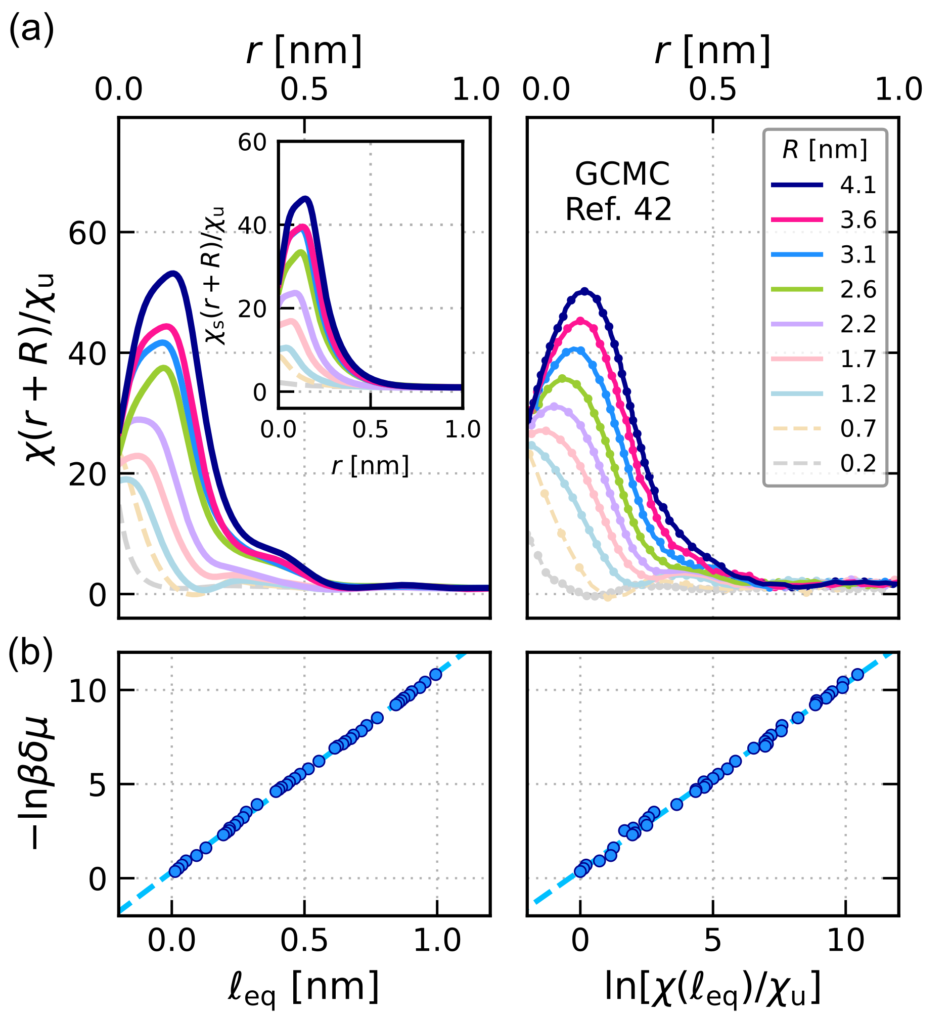
Figure 3: The local compressibility described by an LCW-style cDFT. In (a), we show $\chi(r)$ around different sized hard-sphere solutes, as indicated by the values of $R$ in the legend, centered at the origin. The results from our theory (left) are in good agreement with GCMC simulations from Ref. 42 (right). The inset shows $\chi_{\rm s}(r)$, the contribution from the slowly-varying density, which becomes increasingly important as $R$ increases, though contributions from the rapidly varying part are still significant. All results are for the mW water model ($T=426$ K, $\beta\delta\mu\approx 10^{-3}$, $a=300$ kJ cm³ mol^-2 and $\lambda=0.11$ nm). In (b) we investigate the behavior of $\chi$ near a planar hard wall as $\delta\mu\to 0$. Consistent with a binding potential analysis [43], our theory yields $\ln\chi(\ell_{\rm eq})\sim-\ln\beta\delta\mu$ (right), where $\ell_{\rm eq}$ is the distance of the maximum in $\chi$ from the wall. We also observe $\ell_{\rm eq}\sim-\ln\beta\delta\mu$ (left). Circles show results from the theory and dashed lines indicate the expected scaling relation.

The motivations for our work primarily stem from the desire to develop “semi-implicit” solvation models that retain information on essential solvent correlations. To that end, the results we have presented so far are promising. However, the physics of hydrophobicity is important in its own right. While LCW theory should be considered a seminal contribution in this area, subsequent work from Evans, Wilding and co-workers [44, 45, 46, 47, 48, 42] emphasizes the central role of the critical drying transition that occurs in the limit of a planar substrate with vanishing, or very weak, attractive interactions with the solvent. The extent to which critical drying is captured by LCW theory (or its subsequent lattice-based derivatives [2, 49, 32]) is, however, unclear. Although not equivalent to LCW theory, we can use our cDFT approach to shed light on the extent to which it contains the physics of critical drying.

A key quantity in critical drying phenomena is the local compressibility,

$$\chi(\bm{r})=\bigg{(}\frac{\partial\rho(\bm{r})}{\partial\mu}\bigg{)}_{T},$$ (22)

which in practice is obtained from a finite-difference approximation (see S.I.). Evans, Wilding and co-workers argue that the structure of $\chi(\bm{r})$ provides one of the most robust indicators of hydrophobicity or, more generally, “solvophobicity.”

In the specific case of solvation of hard spheres, $\chi(r)$ should exhibit a pronounced maximum that increases in both magnitude and position with increasing $R$. In Fig. 3(a) we present $\chi(r)$ from our theory, parameterized for the coarse-grained mW water model [50] at $T=426$ K. We see good agreement between the results from our theory compared to grand canonical Monte Carlo (GCMC) simulations by Coe et al.[42] In particular, for the largest solute investigated, $R\approx 4.1$ nm, we see that the maximum value of $\chi(r)$ is over 40 times larger than its bulk counterpart $\chi_{\rm u}$. In the S.I., we also present results where the strength of attractive solute-solvent interactions is decreased, which also compare favorably to GCMC simulations. In the context of an LCW-style theory such as ours, we can also isolate the slowly-varying component of the local compressibility $\chi_{\rm s}(\bm{r})$, by replacing $\rho(\bm{r})$ with $\rho_{\rm s}(\bm{r})$ in Eq. 22. As one might expect, as $R$ increases, so does the significance of $\chi_{\rm s}$. It is clear, however, that contributions from the rapidly-varying density are still important, even for solute sizes that far exceed $R=1$ nm, the colloquial hydrophobic crossover point, as seen in the inset.

A more stringent test of critical drying comes not from comparison to molecular simulation, but from known scaling behaviors of $\chi$ that result from binding potential analyses [43]. Specifically, for a fluid in contact with a planar hard wall, it can be shown that, close to coexistence, $\chi(\ell_{\rm eq})\sim\delta\mu^{-1}$, where $\ell_{\rm eq}$ is the position of the maximum in $\chi$. Moreover, $\ell_{\rm eq}\sim-\ln\delta\mu$. As seen in Fig. 3(b), the LCW-style cDFT approach that we have derived obeys both of these scaling relations. This is far from a trivial result. At face value, the physics of critical drying and the emphasis placed on liquid–vapor interface formation by LCW theory seem unrelated. By recasting the essential underpinnings of LCW theory in the context of cDFT, we begin to paint a unifying picture of these two different views on hydrophobicity.

Multiscale solvation from first principles

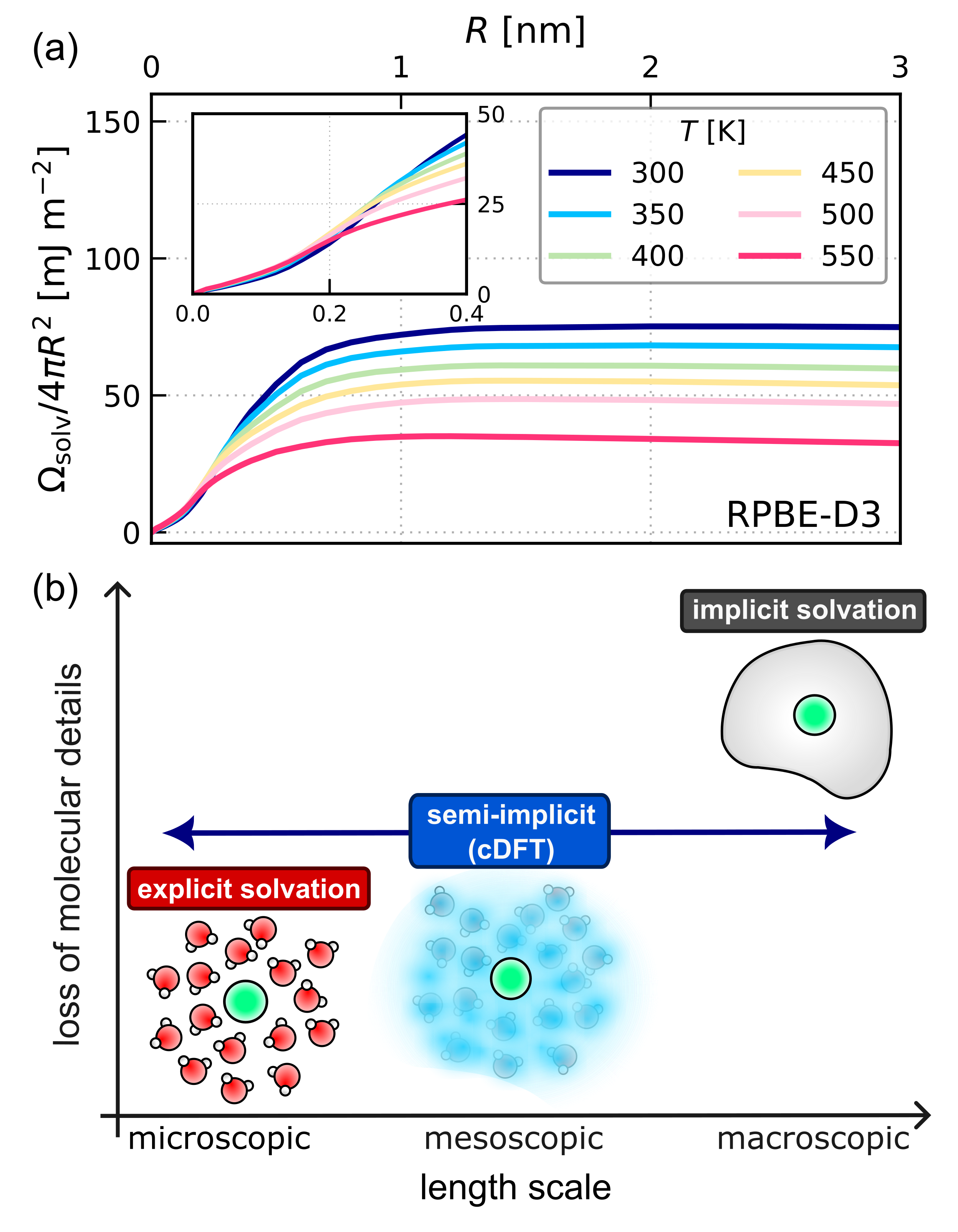
Figure 4: Temperature-dependence of multiscale solvation from first principles. Parameterizing our theory on a first principles representation of water (RPBE-D3), we can predict solvation behavior on length scales inaccessible to molecular simulations. This is demonstrated in (a), where we present $\varOmega_{\rm solv}/4\pi R^{2}$ for hard sphere solutes at different temperatures, as indicated in the legend. The inset highlights the “entropic crossover” that is present in water but not simple liquids [52, 53, 54]. All results are obtained for the liquid at coexistence with $a=300$ kJ cm³ mol^-2 and $\lambda=0.08$ nm. In (b), we summarize the cDFT approach to multiscale modeling. Compared to explicit and implicit solvation approaches, the theory we present instead sacrifices some molecular details, but treats the remaining essential correlations consistently across all length scales.

The physics of critical drying described above is an essential component of hydrophobicity at large length scales. Moreover, it is common to both simple and complex fluids that exhibit solvophobicity. A distinguishing feature of solvophobicity in complex fluids such as water, however, is the “entropic crossover”: for small solutes, $\varOmega_{\rm solv}$ increases with increasing $T$, while for larger solutes it decreases. This behavior has implications for the thermodynamics of protein folding [52], and has been attributed to a competition of microscopic length scales (i.e., solvent reorganization in the first and second solvation shells) that is absent in simple fluids [54]. Here, we will demonstrate that our cDFT approach captures this entropic crossover. Moreover, we will do it from first principles.

Factors of $k_{\rm B}T$ aside, temperature dependence in Eqs. 11 and 16 enters implicitly through $c_{\rm u}^{(2)}$ and $\gamma$. As the approach that we have developed does not assume a simple pairwise additive form for the interatomic potential, the combination of our theory with recent advances in machine-learned interatomic potentials (MLIPs) means we face the exciting prospect of describing, from first principles, the temperature dependence of solvation across the micro-, meso- and macroscales.

For illustrative purposes, we model water with RPBE-D3, a generalized gradient approximation (electronic) functional [55] with dispersion corrections [56]. To obtain $c^{(2)}_{\rm u}$, we have performed our own simulations of bulk water at the liquid density along the coexistence curve, using the MLIP described in Ref. 57, which also provides $\gamma(T)$. In Fig. 4(a), we present results from self-consistent solution of Eqs. 11 and 16 for temperatures ranging from 300 K to 550 K. Note that, in the absence of information in the crossover regime, we have simply taken $m$ to be independent of density. For all temperatures, we observe the hydrophobic crossover. Importantly, this occurs at progressively smaller values of $R$ as $T$ increases; we observe the entropic crossover. These results demonstrate that the LCW-style cDFT that we have developed can be used to faithfully coarse-grain solvent effects while maintaining essential molecular correlations to model phenomenology at a first principles level across a broad range of length scales. This approach is summarized schematically in Fig. 4(b).

Conclusions and Outlook

We have presented a cDFT for the solvation of apolar solutes in water, which is accurate at both small and large length scales. Similar to mDFT, we encode information about the liquid’s small length scale fluctuations by parameterizing our functional on the two-body direct correlation function obtained from simulations of the bulk fluid. In contrast to previous approaches, however, the grand potential that we construct is not based on an expansion around the uniform bulk fluid. Rather, from the outset, our theory acknowledges that the perturbations induced in the solvent density field by large solutes are too severe for the uniform fluid to act as a suitable reference. In this work, we therefore establish a self-consistent cDFT framework that permits the use of an inhomogeneous and slowly-varying density field as a reference system.

The theory that we have outlined is similar in spirit to, and indeed motivated by, the seminal work on the hydrophobic effect by Lum, Chandler and Weeks [15]. By placing the ideas of LCW theory in the context of cDFT, not only do we gain a numerical advantage, but we also provide conceptual insights. For example, the relationship between the “unbalancing potential” and the coarse-grained density field emerges naturally in our theory; the coarse-graining function is the slowly-varying part of a two-body direct correlation function of an inhomogeneous density field. This insight, as we explore in the S.I., justifies a coarse-graining length scale much smaller than the molecular diameter of a water molecule that one might naively expect.

Our approach also allows us to connect the ideas of LCW theory directly with more recent theoretical descriptions of hydrophobicity from Evans, Wilding and co-workers [46, 47]. Specifically, the local compressibility in the presence of large hydrophobes obtained with our approach compares favorably to results obtained by GCMC simulations [42], and we show that its variation with chemical potential obeys known critical scaling behaviors. We also demonstrate that our approach, similar to previous LCW treatments [52], captures the temperature dependence of the hydrophobic effect. It is a curious observation that lattice-based theories of hydrophobicity [49, 32, 59] that aim to improve LCW have emphasized the importance of capillary wave fluctuations; these do not enter explicitly in our theory. Nonetheless, our results for the local compressibility, and the good agreement with solvation free energies obtained from molecular simulations, suggest that we capture the most salient aspects of the interfacial fluctuations necessary to describe hydrophobicity.

A general theory of solvation should also describe the polarization field induced by charged species such as ions. This is a challenging problem beyond the scope of the present study. There are, however, reasons to be optimistic. For example, the mDFT framework already demonstrates that orientational correlations of the bulk fluid can be used to construct density functionals that describe polarization [19]; introducing the results from our work should amount to a straightforward modification of the present mDFT framework. Insights from Weeks’ local molecular field theory may also prove useful in developing new functionals [60, 61, 62, 41, 63, 64] (see Refs. 65, 41 for discussions on the relationship between cDFT and local molecular field theory). In a recent study, Sammüller et al. adopt an entirely different approach by using deep neural networks to construct the free energy functional [66]. Whether such an approach can be used for polar fluids remains to be seen, but it shows great promise. In the context of apolar solvation, our results raise the question whether machine learning can be made easier by first separating the functional into slowly- and rapidly-varying contributions. Notwithstanding the obvious areas for future development, the results of our work demonstrate a significant step toward efficient, and fully first-principles, multiscale modeling of solvation.

Methods

Here we provide a brief overview of the methods used; full details are provided in the S.I. All molecular simulations have been performed with the LAMMPS simulation package[67]. To maintain the temperature, we used the CSVR thermostat[68]. For simulations of SPC/E water [39], long-ranged electrostatic interactions were evaluated using the particle–particle particle–mesh method[69], such that the RMS error in the forces was a factor of $10^{5}$ smaller than the force between two unit charged separated by 0.1 nm[70]. The rigid geometry of the SPC/E water molecules was imposed with the RATTLE algorithm[71]. For simulations of the neural network surrogate model [57] of RPBE-D3 [55, 56], we used the n2p2 package interface[72] with LAMMPS. cDFT calculations were performed with our own bespoke code, which we have made publicly available. Minimization was performed self-consistently using Picard iteration.

Data Availability

Code for minimizing the functionals can be accessed at https://github.com/annatbui/LCW-cDFT. Simulation input files and the direct correlation functions obtained are openly available at the University of Cambridge Data Repository, https://doi.org/10.17863/CAM.104278.

References

- Baldwin [1986] R. L. Baldwin, “Temperature dependence of the hydrophobic interaction in protein folding.” Proceedings of the National Academy of Sciences 83, 8069–8072 (1986).
- ten Wolde and Chandler [2002] P. R. ten Wolde and D. Chandler, “Drying-induced hydrophobic polymer collapse,” Proceedings of the National Academy of Sciences 99, 6539–6543 (2002).
- Dighe and Singh [2019] A. V. Dighe and M. R. Singh, “Solvent fluctuations in the solvation shell determine the activation barrier for crystal growth rates,” Proceedings of the National Academy of Sciences 116, 23954–23959 (2019).
- Chandler [2005] D. Chandler, “Interfaces and the driving force of hydrophobic assembly,” Nature 437, 640–647 (2005).
- Harris and Pettitt [2014] R. C. Harris and B. M. Pettitt, “Effects of geometry and chemistry on hydrophobic solvation,” Proceedings of the National Academy of Sciences 111, 14681–14686 (2014).
- Welch et al. [2016] D. A. Welch, T. J. Woehl, C. Park, R. Faller, J. E. Evans, and N. D. Browning, “Understanding the role of solvation forces on the preferential attachment of nanoparticles in liquid,” ACS Nano 10, 181–187 (2016).
- Patel et al. [2012] A. J. Patel, P. Varilly, S. N. Jamadagni, M. F. Hagan, D. Chandler, and S. Garde, “Sitting at the edge: How biomolecules use hydrophobicity to tune their interactions and function,” The Journal of Physical Chemistry B 116, 2498–2503 (2012).
- Evans, Stewart, and Wilding [2019] R. Evans, M. C. Stewart, and N. B. Wilding, “A unified description of hydrophilic and superhydrophobic surfaces in terms of the wetting and drying transitions of liquids,” Proceedings of the National Academy of Sciences 116, 23901–23908 (2019).
- Levy and Gallicchio [1998] R. M. Levy and E. Gallicchio, “Computer simulations with explicit solvent: Recent progress in the thermodynamic decomposition of free energies and in modeling electrostatic effects,” Annual Review of Physical Chemistry 49, 531–567 (1998).
- Chothia [1974] C. Chothia, “Hydrophobic bonding and accessible surface area in proteins,” Nature 248, 338–339 (1974).
- Sharp and Honig [1990] K. A. Sharp and B. Honig, “Calculating total electrostatic energies with the nonlinear Poisson-Boltzmann equation,” The Journal of Physical Chemistry 94, 7684–7692 (1990).
- Sharp et al. [1991] K. A. Sharp, A. Nicholls, R. F. Fine, and B. Honig, “Reconciling the magnitude of the microscopic and macroscopic hydrophobic effects,” Science 252, 106–109 (1991).
- Cramer and Truhlar [1992] C. J. Cramer and D. G. Truhlar, “An SCF solvation model for the hydrophobic effect and absolute free energies of aqueous solvation,” Science 256, 213–217 (1992).
- Wagoner and Baker [2006] J. A. Wagoner and N. A. Baker, “Assessing implicit models for nonpolar mean solvation forces: The importance of dispersion and volume terms,” Proceedings of the National Academy of Sciences 103, 8331–8336 (2006).
- Lum, Chandler, and Weeks [1999] K. Lum, D. Chandler, and J. D. Weeks, “Hydrophobicity at small and large length scales,” The Journal of Physical Chemistry B 103, 4570–4577 (1999).
- Zhao et al. [2011] S. Zhao, R. Ramirez, R. Vuilleumier, and D. Borgis, “Molecular density functional theory of solvation: From polar solvents to water,” The Journal of Chemical Physics 134, 194102 (2011).
- Jeanmairet et al. [2013] G. Jeanmairet, M. Levesque, R. Vuilleumier, and D. Borgis, “Molecular density functional theory of water,” The Journal of Physical Chemistry Letters 4, 619–624 (2013).
- Jeanmairet, Levesque, and Borgis [2013] G. Jeanmairet, M. Levesque, and D. Borgis, “Molecular density functional theory of water describing hydrophobicity at short and long length scales,” The Journal of Chemical Physics 139, 154101 (2013).
- Jeanmairet et al. [2016] G. Jeanmairet, N. Levy, M. Levesque, and D. Borgis, “Molecular density functional theory of water including density–polarization coupling,” Journal of Physics: Condensed Matter 28, 244005 (2016).
- Borgis et al. [2020] D. Borgis, S. Luukkonen, L. Belloni, and G. Jeanmairet, “Simple parameter-free bridge functionals for molecular density functional theory. Application to hydrophobic solvation,” The Journal of Physical Chemistry B 124, 6885–6893 (2020).
- Evans [1979] R. Evans, “The nature of the liquid-vapour interface and other topics in the statistical mechanics of non-uniform, classical fluids,” Advances in Physics 28, 143–200 (1979).
- Evans [1992] R. Evans, Fundamentals of inhomogeneous fluids, edited by D. Henderson (Dekker, New York, 1992).
- Lutsko [2010] J. F. Lutsko, “Recent developments in classical density functional theory,” Advances in Chemical Physics, 1–92 (2010).
- Rosenfeld [1989] Y. Rosenfeld, “Free-energy model for the inhomogeneous hard-sphere fluid mixture and density-functional theory of freezing,” Phys. Rev. Lett. 63, 980–983 (1989).
- Tarazona [2000] P. Tarazona, “Density functional for hard sphere crystals: A fundamental measure approach,” Phys. Rev. Lett. 84, 694–697 (2000).
- Roth et al. [2002] R. Roth, R. Evans, A. Lang, and G. Kahl, “Fundamental measure theory for hard-sphere mixtures revisited: the White Bear version,” Journal of Physics: Condensed Matter 14, 12063 (2002).
- Hansen and McDonald [2013] J. Hansen and I. McDonald, Theory of Simple Liquids: with Applications to Soft Matter (Elsevier Science, 2013).
- Sergiievskyi et al. [2017] V. Sergiievskyi, M. Levesque, B. Rotenberg, and D. Borgis, “Solvation in atomic liquids: connection between Gaussian field theory and density functional theory,” Condensed Matter Physics, 20, 333005 (2017).
- Huang, Geissler, and Chandler [2001] D. M. Huang, P. L. Geissler, and D. Chandler, “Scaling of hydrophobic solvation free energies,” The Journal of Physical Chemistry B 105, 6704–6709 (2001).
- Huang and Chandler [2002] D. M. Huang and D. Chandler, “The hydrophobic effect and the influence of solute-solvent attractions,” The Journal of Physical Chemistry B 106, 2047–2053 (2002).
- Sedlmeier and Netz [2012] F. Sedlmeier and R. R. Netz, “The spontaneous curvature of the water-hydrophobe interface,” The Journal of Chemical Physics 137, 135102 (2012).
- Vaikuntanathan and Geissler [2014] S. Vaikuntanathan and P. L. Geissler, “Putting water on a lattice: The importance of long wavelength density fluctuations in theories of hydrophobic and interfacial phenomena,” Phys. Rev. Lett. 112, 020603 (2014).
- Evans, Tarazona, and Marconi [1983] R. Evans, P. Tarazona, and U. M. B. Marconi, “On the failure of certain integral equation theories to account for complete wetting at solid-fluid interfaces,” Molecular Physics 50, 993–1011 (1983).
- Borgis et al. [2021] D. Borgis, S. Luukkonen, L. Belloni, and G. Jeanmairet, “Accurate prediction of hydration free energies and solvation structures using molecular density functional theory with a simple bridge functional,” The Journal of Chemical Physics 155, 024117 (2021).
- Weeks [2002] J. D. Weeks, “Connecting local structure to interface formation: A molecular scale van der Waals theory of nonuniform liquids,” Annual Review of Physical Chemistry 53, 533–562 (2002).
- Chandler [1993] D. Chandler, “Gaussian field model of fluids with an application to polymeric fluids,” Phys. Rev. E 48, 2898–2905 (1993).
- Vega and de Miguel [2007] C. Vega and E. de Miguel, “Surface tension of the most popular models of water by using the test-area simulation method,” The Journal of Chemical Physics 126, 154707 (2007).
- Fujita and Yamamoto [2017] T. Fujita and T. Yamamoto, “Assessing the accuracy of integral equation theories for nano-sized hydrophobic solutes in water,” The Journal of Chemical Physics 147, 014110 (2017).
- Berendsen, Grigera, and Straatsma [1987] H. J. C. Berendsen, J. R. Grigera, and T. P. Straatsma, “The missing term in effective pair potentials,” The Journal of Physical Chemistry 91, 6269–6271 (1987).
- Katsov and Weeks [2001] K. Katsov and J. D. Weeks, “On the mean field treatment of attractive interactions in nonuniform simple fluids,” The Journal of Physical Chemistry B 105, 6738–6744 (2001).
- Remsing, Liu, and Weeks [2016] R. C. Remsing, S. Liu, and J. D. Weeks, “Long-ranged contributions to solvation free energies from theory and short-ranged models,” Proceedings of the National Academy of Sciences 113, 2819–2826 (2016).
- Coe, Evans, and Wilding [2023] M. K. Coe, R. Evans, and N. B. Wilding, “Understanding the physics of hydrophobic solvation,” The Journal of Chemical Physics 158, 034508 (2023).
- Evans, Stewart, and Wilding [2017] R. Evans, M. C. Stewart, and N. B. Wilding, “Drying and wetting transitions of a Lennard-Jones fluid: Simulations and density functional theory,” The Journal of Chemical Physics 147, 044701 (2017).
- Evans and Stewart [2015] R. Evans and M. C. Stewart, “The local compressibility of liquids near non-adsorbing substrates: a useful measure of solvophobicity and hydrophobicity?” Journal of Physics: Condensed Matter 27, 194111 (2015).
- Evans and Wilding [2015] R. Evans and N. B. Wilding, “Quantifying density fluctuations in water at a hydrophobic surface: Evidence for critical drying,” Phys. Rev. Lett. 115, 016103 (2015).
- Evans, Stewart, and Wilding [2016] R. Evans, M. C. Stewart, and N. B. Wilding, “Critical drying of liquids,” Phys. Rev. Lett. 117, 176102 (2016).
- Coe, Evans, and Wilding [2022a] M. K. Coe, R. Evans, and N. B. Wilding, “Density depletion and enhanced fluctuations in water near hydrophobic solutes: Identifying the underlying physics,” Phys. Rev. Lett. 128, 045501 (2022a).
- Coe, Evans, and Wilding [2022b] M. K. Coe, R. Evans, and N. B. Wilding, “The coexistence curve and surface tension of a monatomic water model,” The Journal of Chemical Physics 156, 154505 (2022b).
- Varilly, Patel, and Chandler [2011] P. Varilly, A. J. Patel, and D. Chandler, “An improved coarse-grained model of solvation and the hydrophobic effect,” The Journal of Chemical Physics 134, 074109 (2011).
- Molinero and Moore [2009] V. Molinero and E. B. Moore, “Water modeled as an intermediate element between carbon and silicon,” The Journal of Physical Chemistry B 113, 4008–4016 (2009).
- Note [1] K corresponds to , with the critical point of mW at K (from Ref. \rev@citealpnumCoe2022b).
- Huang and Chandler [2000] D. M. Huang and D. Chandler, “Temperature and length scale dependence of hydrophobic effects and their possible implications for protein folding,” Proceedings of the National Academy of Sciences 97, 8324–8327 (2000).
- Ashbaugh [2009] H. S. Ashbaugh, “Blowing bubbles in Lennard-Jonesium along the saturation curve,” The Journal of Chemical Physics 130, 204517 (2009).
- Dowdle et al. [2013] J. R. Dowdle, S. V. Buldyrev, H. E. Stanley, P. G. Debenedetti, and P. J. Rossky, “Temperature and length scale dependence of solvophobic solvation in a single-site water-like liquid,” The Journal of Chemical Physics 138, 064506 (2013).
- Hammer, Hansen, and Nørskov [1999] B. Hammer, L. B. Hansen, and J. K. Nørskov, “Improved adsorption energetics within density-functional theory using revised Perdew-Burke-Ernzerhof functionals,” Phys. Rev. B 59, 7413–7421 (1999).
- Grimme et al. [2010] S. Grimme, J. Antony, S. Ehrlich, and H. Krieg, “A consistent and accurate ab initio parametrization of density functional dispersion correction (DFT-D) for the 94 elements H-Pu,” The Journal of Chemical Physics 132, 154104 (2010).
- Wohlfahrt, Dellago, and Sega [2020] O. Wohlfahrt, C. Dellago, and M. Sega, “Ab initio structure and thermodynamics of the RPBE-D3 water/vapor interface by neural-network molecular dynamics,” The Journal of Chemical Physics 153, 144710 (2020).
- Note [2] For a Lennard–Jones fluid, this relationship between the coarse-grained density and the correlation function is identical to that specified by Weeks in the context of local molecular field theory [35], if we use a random phase approximation for the slowly-varying functional . However, it is clear that the overall functional that we obtain is not a simple mean field approximation.
- Vaikuntanathan et al. [2016] S. Vaikuntanathan, G. Rotskoff, A. Hudson, and P. L. Geissler, “Necessity of capillary modes in a minimal model of nanoscale hydrophobic solvation,” Proceedings of the National Academy of Sciences 113, E2224–E2230 (2016).
- Rodgers and Weeks [2008a] J. M. Rodgers and J. D. Weeks, “Local molecular field theory for the treatment of electrostatics,” Journal of Physics: Condensed Matter 20, 494206 (2008a).
- Rodgers and Weeks [2009] J. M. Rodgers and J. D. Weeks, “Accurate thermodynamics for short-ranged truncations of Coulomb interactions in site-site molecular models,” The Journal of Chemical Physics 131, 244108 (2009).
- Rodgers and Weeks [2008b] J. M. Rodgers and J. D. Weeks, “Interplay of local hydrogen-bonding and long-ranged dipolar forces in simulations of confined water,” Proc. Natl. Acad. Sci. 105, 19136–19141 (2008b).
- Gao, Remsing, and Weeks [2020] A. Gao, R. C. Remsing, and J. D. Weeks, “Short solvent model for ion correlations and hydrophobic association,” Proc. Natl. Acad. Sci. 117, 1293–1302 (2020).
- Cox [2020] S. J. Cox, “Dielectric response with short-ranged electrostatics,” Proceedings of the National Academy of Sciences 117, 19746–19752 (2020).
- Archer and Evans [2013] A. J. Archer and R. Evans, “Relationship between local molecular field theory and density functional theory for non-uniform liquids,” The Journal of Chemical Physics 138, 014502 (2013).
- Sammüller et al. [2023] F. Sammüller, S. Hermann, D. de las Heras, and M. Schmidt, “Neural functional theory for inhomogeneous fluids: Fundamentals and applications,” Proceedings of the National Academy of Sciences 120, e2312484120 (2023).
- Thompson et al. [2022] A. P. Thompson, H. M. Aktulga, R. Berger, D. S. Bolintineanu, W. M. Brown, P. S. Crozier, P. J. in ’t Veld, A. Kohlmeyer, S. G. Moore, T. D. Nguyen, R. Shan, M. J. Stevens, J. Tranchida, C. Trott, and S. J. Plimpton, “LAMMPS - a flexible simulation tool for particle-based materials modeling at the atomic, meso, and continuum scales,” Computer Physics Communications 271, 108171 (2022).
- Bussi, Donadio, and Parrinello [2007] G. Bussi, D. Donadio, and M. Parrinello, “Canonical sampling through velocity rescaling,” The Journal of Chemical Physics 126, 014101 (2007).
- Hockney and Eastwood [1988] R. Hockney and J. Eastwood, Computer Simulation Using Particles (Adam-Hilger, 1988).
- Kolafa and Perram [1992] J. Kolafa and J. W. Perram, “Cutoff errors in the Ewald summation formulae for point charge systems,” Molecular Simulation 9, 351–368 (1992).
- Andersen [1983] H. C. Andersen, “Rattle: A “velocity” version of the shake algorithm for molecular dynamics calculations,” Journal of Computational Physics 52, 24–34 (1983).
- Singraber, Behler, and Dellago [2019] A. Singraber, J. Behler, and C. Dellago, “Library-based LAMMPS implementation of high-dimensional neural network potentials,” Journal of Chemical Theory and Computation 15, 1827–1840 (2019).