Quantum Normalizing Flows for Anomaly Detection

Abstract

A Normalizing Flow computes a bijective mapping from an arbitrary distribution to a predefined (e.g. normal) distribution. Such a flow can be used to address different tasks, e.g. anomaly detection, once such a mapping has been learned. In this work we introduce Normalizing Flows for Quantum architectures, describe how to model and optimize such a flow and evaluate our method on example datasets. Our proposed models show competitive performance for anomaly detection compared to classical methods, e.g. based on isolation forests, the local outlier factor (LOF) or single-class SVMs, while being fully executable on a quantum computer.

I Introduction

Anomaly detection is the task to identify data points, entities or events that fall outside a normal range. Thus an anomaly is a data point that deviates from its expectation or the majority of the observations. Applications are in the domains of cyber-security EVANGELOU2020101941 , medicine FERNANDO202067 , machine vision BroRud2023 , (financial) fraud detection Reddy21 or production RudWan2021a . In this work we assume that only normal data is available during training. Such an assumption is valid e.g. in production environments where many positive examples are available and events happen rarely which lead to faulty examples. During inference, the model has to differ between normal and anomalous samples. This is also termed semi-supervised anomaly detection ruff2020deep , novelty detection pmlr-v5-scott09a ; Schoelkopf99 or one-class classification Amer13 .

In this work we will make use of Normalizing Flows Kobyzev2020 for anomaly detection. A Normalizing Flow (NF) is a transformation of an arbitrary distribution, e.g. coming from a dataset to a provided probability distribution (e.g., a normal distribution). The deviation from an expected normal distribution can then be used as anomaly score for anomaly detection. A property of normalizing flows is the bijectivity, thus a NF can be evaluated as forward and backward path, an aspect which is trivial for quantum gates which can be represented as unitary matrices. Another aspect is that on a quantum computer the output is always a distribution of measurements. This distribution can be directly compared to the target distribution by using a KL-divergence measure for evaluation. In general this step will require sampling. We therefore propose to optimize a NF using quantum gates and use the resulting architectures for anomaly detection. In the experiments, we compare the resulting quantum architectures with standard approaches for anomaly detection, e.g. based on isolation forests, local outlier factors (LOF) and one-class support vector machines (SVMs) and show a competitive performance. We also demonstrate how to use the Quantum Normalizing Flow as generative model by sampling from the target distribution and evaluating the backward flow. For the optimization of the quantum gate order, we rely on quantum architecture search and directly optimize the gate selection and order for the KL-divergence as loss function.

Our contributions can be summarized as follows:

1. We propose Quantum Normalizing Flows to compute a bijective mapping from data samples to a normal distribution

2. Our optimized models are used for anomaly detection and are evaluated and compared to classical methods demonstrating their competitive performance.

3. Our optimized models are used as generative model by sampling from the target distribution and evaluating the backward flow.

4. Our source code for optimization will be made publicly available .

II Preliminaries

In this section we give a brief overview of the quantum framework we use later, a summary on Normalizing Flows, and provide an overview of existing quantum driven and classical anomaly detection frameworks. Three classical and well established methods are later used for a direct comparison with our proposed Quantum-Flow algorithm, namely isolation forests, local outlier factors (LOFs) and single-class SVMs.

II.1 Quantum Gates and Circuits

We focus on the setting where our quantum information processing device is comprised of a set of $N$ logical qubits, arranged as a quantum register (see, e.g., 10.5555/1206629 for further details). Thus we use a Hilbert space of our system $\mathcal{H}\equiv(\mathbb{C}^{2})^{\otimes N}\cong\mathbb{C}^{2^{N}}$ as algebraic embedding. Therefore, e.g., a quantum state vector of a 5-qubit register is a unit vector in $\mathbb{C}^{2^{5}}=\mathbb{C}^{32}$. We further assume that the system is not subject to decoherence or other external noise.

Quantum gates are the basic building blocks of quantum circuits, similar to logic gates in digital circuits Selinger2004a . According to the axioms of quantum mechanics, quantum logic gates are represented by unitary matrices so that a gate acting on $N$ qubits is represented by a $2^{N}\times 2^{N}$ unitary matrix, a quantum code comprises of a set of such gates which in return are evaluated as a series of matrix multiplications. A quantum circuit of length $L$ is therefore described by an ordered tuple $(O(1),O(2),\ldots,O(L))$ of quantum gates; the resulting unitary operation $U$ implemented by the circuit is the product

$$U=O(L)O(L-1)\cdots O(1).$$ (1)

Standard quantum gates include the Pauli-($X$, $Y$, $Z$) operations, as well as Hadamard-, cnot-, swap-, phase-shift-, and toffoli-gates, all of which are expressible as standardised unitary matrices nielsen2010quantum . The action of a quantum gate is extended to a register of any size exploiting the tensor product operation in the standard way. Even though some gates do not involve additional variables, however, e.g., a phase-shift gate $R_{X}(\theta)$ applies a complex rotation and involves the rotation angle $\theta$ as free parameter.

II.2 Normalizing Flows

A Normalizing Flow (NF) is a transformation of a provided (simple) probability distribution (e.g., a normal distribution) into an arbitrary distribution by a sequence of invertible mappings. They have been introduced by Rezende and Mohamed nf as a generative model to generate examples from sampling a normal distribution.

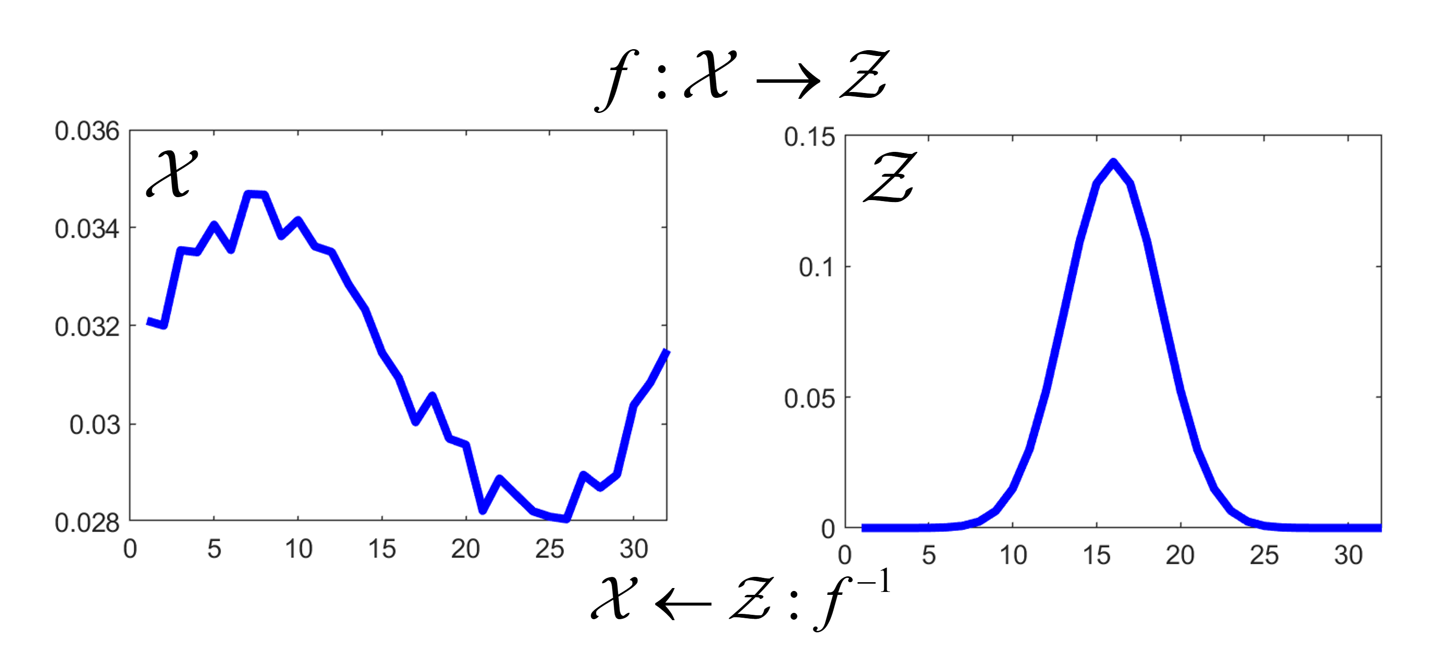
Figure 1: Visualization of a normalizing flow $f$. It is a bijective transformation $f$ of an arbitrary distribution to e.g. a normal distribution.

Compared to other generative models such as variational autoencoders (VAEs)  vae or Generative Adversarial Networks (GANs) gan a NF comes along with the property that it maps bijectively and is bidirectionally executable. Thus, the input dimension is the same as the output dimension. Usually, they are optimized via maximum likelihood training and the minimization of a KL-divergence measure. Given two probability distributions $P$ and $Q$, the Kullback-Leibler-divergence (KL-divergence) or relative entropy is a dissimilarity measure for two distributions,

$$D_{KL}(P\parallel Q) = \sum_{x\in\mathcal{X}}p(x)\log\left(\frac{p(x)}{q(x)}\right)$$ (2)

Since the measure is differentiable, it has been frequently used in the context of neural network models for a variety of downstream tasks such as image generation, noise modelling, video generation, audio generation, graph generation and more Kobyzev2020 . After the training process, a learned NF can be used in two ways, either as generator or likelihood estimator. The forward pass $f:\mathcal{X}\rightarrow\mathcal{Z}$ allows for computing the likelihood of observed data points given the target distribution $p_{Z}$ (e.g. unit Gaussian). The backward pass $f^{-1}:\mathcal{Z}\rightarrow\mathcal{X}$ allows for generating new samples in the original space $\mathcal{X}$ by sampling from the latent space $\mathcal{Z}$ according to the estimated densities as in kingma2018glow ; tomINN . Figure 1 visualizes the change of variables given the source distribution $p_{\mathcal{X}}$ and the target distribution $p_{\mathcal{Z}}$.

Several neural network architectures for such transformations have been proposed in the past realnvp ; kingma ; germain ; maf . Since quantum gates are by definition expressable as unitary matrices which are invertible, a quantum gate fulfills the basic properties of an invertible and bijective mapping. Thus, we aim for optimizing a quantum architecture providing the desired Normalizing Flow transformation and use the likelihood estimation from the forward pass to compute an anomaly score for anomaly detection.

II.3 Anomaly Detection

Anomaly detection is the task to identify data points, entities or events that fall outside an expected range. Anomaly detection is applicable in many domains and can be seen as a subarea of unsupervised machine learning. In our setting we focus on a setting where only positive examples are provided which is also termed one-class classification or novelty detection. In the following we will first summarize recent quantum approaches for anomaly detection and will then introduce in more detail three reference methods we will use in our experiments.

II.3.1 Quantum anomaly detection

One of the first approaches to formulate anomaly detection on quantum computers has been proposed in PhysRevA.97.042315 . The authors mainly build up on a kernel PCA and a one-class support vector machine, one of the approaches we will introduce in more detail later. So-called change point detection has been analyzed in PhysRevLett.119.140506 ; PhysRevA.98.052305 ; fanizza2023ultimate . In PhysRevA.99.052310 , Liang et.al. propose anomaly detection using density estimation. Therefore it is assumed that the data follows a specific type of distribution, in its simplest form a Gaussian mixture model. In GUO2023129018 the Local Outlier Factor algorithm (LOF algorithm) LOF2000 has been used and remapped to a quantum formulation. As explained later, the LOF algorithm contains three steps, (a) determine the k-distance neighborhood for each data point $x$, (b) compute the local reachability density of $x$, and (c) calculate the local outlier factor of $x$ to judge whether $x$ is abnormal. In GUO2022127936 the authors propose an efficient quantum anomaly detection algorithm based on density estimation which is driven from amplitude estimation. They show that their algorithm achieves exponential speed up on the number of training data points $M$ over its classical counterpart. Besides fundamental theoretical concepts, many works do not show any experiments on real datasets and are therefore often limited to very simple and artificial examples. Also the generated quantum codes can require a large amount of qubits and they lead to reasonable large code lengths which is suboptimal for real-world scenarios.

In the following we will summarize three classical and well established methods which we will later use for a direct comparison to our proposed Quantum-Flow.

II.3.2 Isolation forests

An isolation forest is an algorithm for anomaly detection which has been initially proposed by Liu et.al. liu2008isolation . It detects anomalies using characteristics of anomalies, i.e. being few and different. The idea behind the isolation forest algorithm is that anomalous data points are easier to separate from the rest of the data. In order to isolate a data point, the algorithm generates partitions on the samples by randomly selecting an attribute and then randomly selecting a split value in a valid parameter range. The recursive partitioning leads to a tree structure and the required number of partitions to isolate a point corresponds to the length of the path in the tree. Repeating this strategy leads to an isolation forest and finally, all path lengths in the forest are used to determine an anomaly score. The isolation forest algorithm computes the anomaly score s(x) of an observation x by normalizing the path length h(x):

$$s(x) = 2^{-\frac{E[h(x)]}{c(n)}}$$ (3)

where $E[h(x)]$ is the average path length over all isolation trees in the isolation forest, and $c(n)$ is the average path length of unsuccessful searches in a binary search tree of $n$ observations.

The algorithm has been extended in Liu2010 and Talagala2021 to address clustered and high dimensional data. Another extension is anomaly detection for dynamic data streams using random cut forests, which has been presented in pmlr-v48-guha16 .

II.3.3 Local outlier factor (LOF)

The Local Outlier Factor algorithm (LOF algorithm) has been introduced in LOF2000 . Outlier detection is based on the relative density of a data point with respect to the surrounding neighborhood. It uses the $k$-nearest neighbor and can be summarized as

$$LOF_{k}(p) = \frac{1}{|N_{k}(p)|}\sum_{o\in N_{k}(p)}\frac{lrd_{k}(o)}{lrd_{k}(p)}$$ (4)

Here, $lrd$ denotes the local reachability density, $N_{k}(p)$ represents the $k$-nearest neighbor of an observation $p$. The reachability distance of observation $p$ with respect to observation $o$ is defined as

$$\tilde{d}_{k}(p,o) = \max(d_{k}(o),d(p,o))$$ (5)

where $d_{k}(o)$ is the $k$th smallest distance among the distances from the observation $o$ to its neighbors and $d(p,o)$ denotes the distance between observation $p$ and observation $o$. The local reachability density of observation $p$ is reciprocal to the average reachability distance from observation p to its neighbors.

$$lrd_{k}(p) = \frac{1}{\frac{\sum_{o\in N_{k}(p)}\tilde{d}_{k}(p,o)}{|N_{k}(p)|}}$$ (6)

The LOF can be computed on different distance metrics, e.g. an Euclidean, mahalanobis, city block, minkowsky distance or others.

II.3.4 Single Class SVM

Single class support vector machines (SVMs) for novelty detection have been proposed in Schoelkopf99 . The idea is to estimate a function $f$ which is positive on a simple set $S$ and negative on the complement, thus the probability that a test point drawn from a probability distribution $P$ lies outside of $S$ equals some a priori specified $v$ between $0$ and $1$. Let $x_{i}\in\mathbb{R}^{N}$ denote the training data and $\Phi$ be a feature map into a dot product space $F$ such that a kernel expression

$$k(x,y) = \Phi(x)^{T}\Phi(y)$$ (7)

can be used to express a non-linear decision plane in a linear fashion, which is also known as kernel trick Aizerman67 . The following formulation optimizes the parameters $w$ and $\rho$ and returns a function $f$ that takes the value $+1$ in a small region capturing most of the data points, and $-1$ elsewhere. The objective function can be expressed as quadratic program of the form

$$\textrm{min}_{w\in F,\xi\in\mathbb{R}^{t},\rho\in\mathbb{R}} \frac{1}{2}\|w\|^{2}+\frac{1}{v^{l}}\sum_{i}\xi_{i}-\rho$$ (8)

s.t. $$(w^{T}\Phi(x_{i}))\geq\rho-\xi_{i},\hskip 14.22636pt\xi\geq 0$$

The nonzero slack variables $\xi_{i}$ act as penalizer in the objective function. If $w$ and $\rho$ can explain the data, the decision function

$$f(x) = \textrm{sgn}((w^{T}\Phi(x))-\rho)$$ (10)

will be positive for most examples $x_{i}$, while the support vectors in $\|w\|$ will be minimized, thus the tradeoff between an optimal encapsulation of the training data and accepting outlier in the data is controlled by $v$. Expanding $f$ by using the dual problem leads to

$$f(x) = \textrm{sgn}((w^{T}\Phi(x))-\rho)$$ (11)

$$= \textrm{sgn}\left(\sum_{i}\alpha_{i}k(x_{i},x)-\rho\right)$$ (12)

which indicates the support vectors of the decision boundary with nonzero $\alpha_{i}$s. This basic formulation has been frequently used in anomaly detection and established as a well performing algorithm Amer13 ; NIPS2007_013a006f . For more details in linear and quadratic programming we refer to murty1983 ; Nguyen2012 ; Paul09 ; Bod2023a .

III Method

In the following we present the proposed method and conducted experiments. The section starts with a brief summary of the used optimization strategy based on quantum architecture search, continues with the evaluation metrics, based on a ROC curve and presents the proposed quantum flow anomaly detection framework. The evaluation is perfomed on two selected datasets, the iris dataset and the wine dataset. Here, we will compare the outcome of our optimized quantum flow with the performance of isolation forests, the LOF and a single class SVM.

III.1 Optimization

Optimization is based on quantum architecture search. The name is borrowed and adapted from Neural Architecture Search (NAS) Miikkulainen2020 ; xie2018snas , which is devoted to the study and hyperparameter tuning of neural networks. Many QAS-variants are focussed on discrete optimization and exploit optimization strategies for non-differentiable optimization criteria. In the past, variants of Gibbs sampling PhysRevResearchLi20 , evolutional approaches 9870269 , genetic algorithms RasconiOddi2019 ; PhysRevLett116.230504 and neural-network based predictors Zhang2021 have been suggested. A recent survey on QAS can be found in Zhu23ICACS . For this work, we rely on the former work RosOsb2023a proposing Monte Carlo Graph Search. The optimized loss function is in our case the Kullback-Leibler divergence, $D_{KL}(P\parallel Q)$ (see Equation (2)).

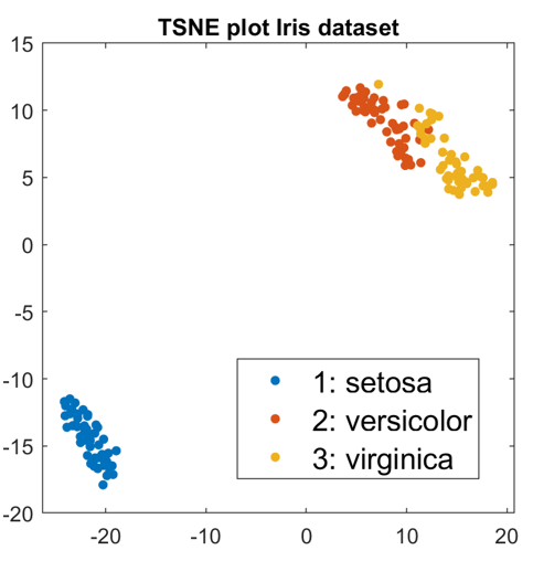
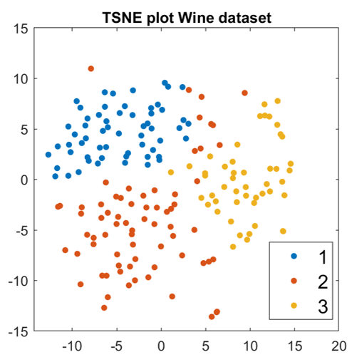
Figure 2: TSNE-plot of the iris (top) and wine (bottom) datasets. The iris dataset has been selected since one class separates very easy from the rest, whereas the remaining classes are more similar and overlapping. The second class of the wine dataset is spreading into the classes one and three.

III.2 Evaluation Metrics

To compare the performance of different algorithms, the area under the ROC-curve hanley1982meaning is a common measure. To summarise, a ROC curve (receiver operating characteristic curve) is a graph showing the performance of a classification model at all classification thresholds. In our case, the classification threshold is the anomaly score of the algorithm and the x-y axes contains the false-positive rate (x-axis) versus the true-positive rate (y-axis) for all possible anomaly thresholds. The area under the generated curve is the AUROC which is 1 in the optimal case when all examples are correctly classified while producing no false positives. For anomaly detection, the AUROC is the standard measure in literature for the following reasons, (a) the AUROC is scale-invariant. It measures how well predictions are ranked, rather than their absolute values and (b) the AUROC is classification-threshold-invariant. It measures the quality of the model’s predictions irrespective of what classification threshold is chosen.

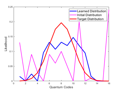
Figure 3: Optimized Normalizing Flow from an input distribution (magenta) to a target distribution (blue) and the comparison to a discrete Gaussian distribution.

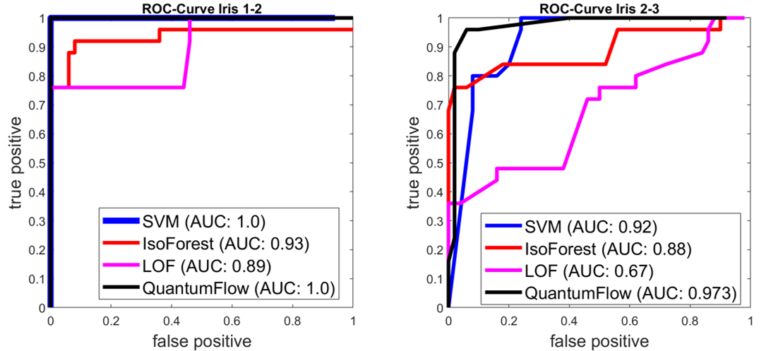
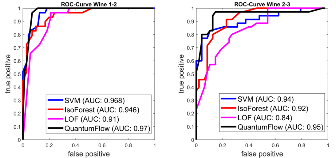
Figure 4: The resulting ROC-Curves and the aurea-under the ROC-Curve (AUROC) for different settings on the Iris and Wine dataset.

III.3 Quantum Flow Anomaly Detection

Dataset Dim BDim qubits # Train # Test Iris 1-2 4 12 4 25 25/50 Iris 2-3 4 12 4 25 25/50 Wine 1-2 14 28 5 29 29/71 Wine 2-3 14 28 5 35 35/48

Table 1: Datasets overview, the used normal class, the anomal class and train/test splits.

For the experiments, the classical wine and iris datasets were used. The datasets present multicriterial classification tasks, with three categories for the wine dataset, and three for the iris dataset. The datasets are all available at the UCI repository Dua:2019 . To model an anomaly detection task using a quantum circuit, first the data is encoded as a higher-dimensional binary vector. Taking the iris dataset as a toy example, it consists of $4$ dimensional data encoding sepal length, sepal width, petal length and petal width. A kMeans clustering on each dimension with $k=3$ is used on the training data. Thus, every datapoint can be encoded in a $4\times 3=12-$dimensional binary vector which contains exactly $4$ non-zero entries. The iris dataset contains three categories, samely setosa, versicolor and virginica. We select 50% of data points from one class (e.g. setosa) for training and use the remaining datapoints, as well as a second class (e.g. virginica) for testing. Thus, the setosa test cases should be true positives, whereas the virginica should be correctly labeled as anomalies. Figure 2 shows a TSNE-plot of the iris dataset on the top and and a TSNE plot of the wine dataset on the bottom. The iris dataset has been selected since one class separates very easily from the rest, whereas the remaining classes are more similar and overlapping. The second class of the wine dataset is spreading into the classes one and three, here the anomaly detection is also challenging. These properties will also be reflected in the anomaly scores in the experiments.

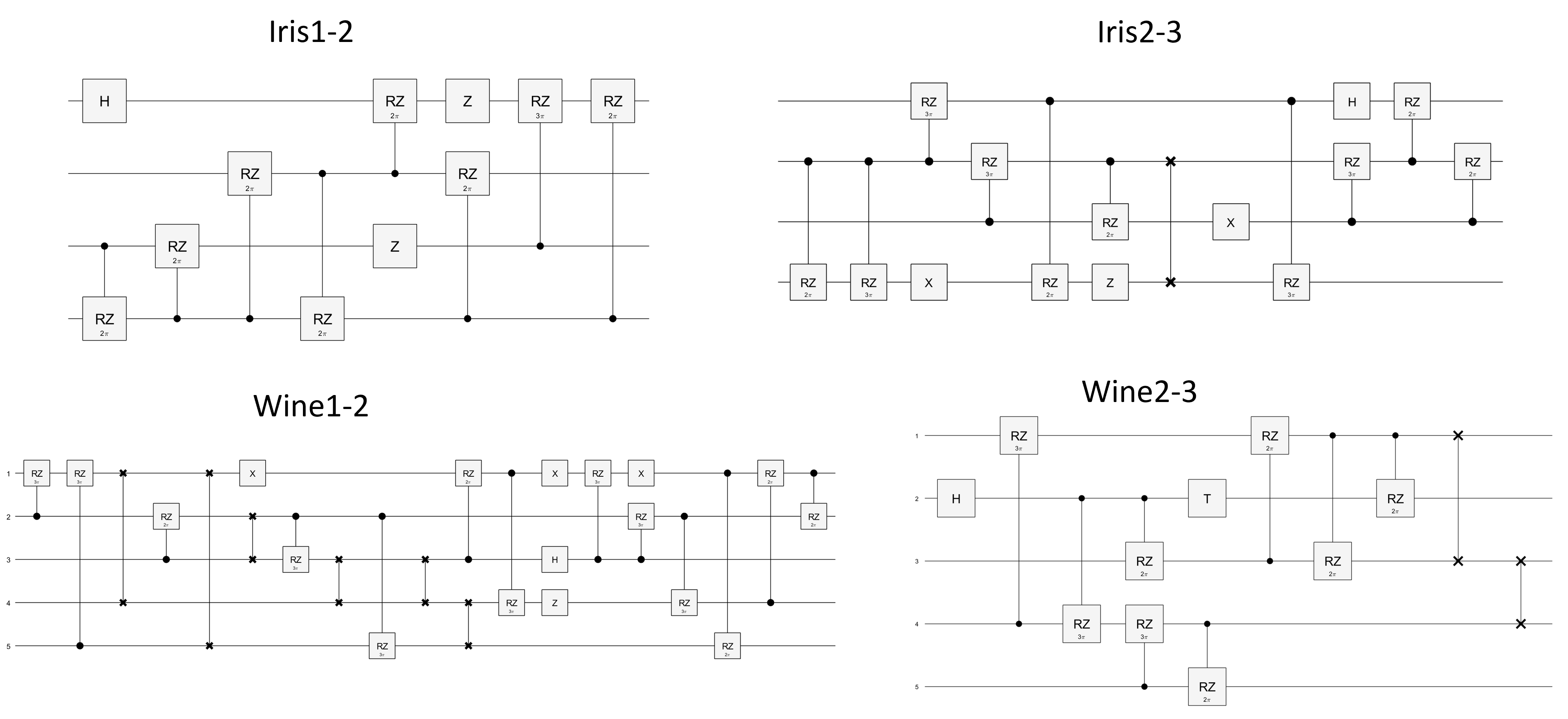
Figure 5: Obtained quantum codes after optimization. Despite the competitive performance the resulting codes are reasonable small and efficient.

For the classically computed quantum architecture search, we compute the discrete distribution $Nhist$ as the normalized histogram of the training dataset as input and use a binomial distribution ($p=0.5$) as target.

$$X\sim p(X==k) \sim Nhist(k,n)$$ (13)

$$Y\sim p(Y==k) \sim \binom{n}{k}p^{k}(1-p)^{n-k}$$

The optimization task is to find an ordered set of quantum gates (see Equation (1)) which lead a unitary matrix $U=O(L)\mbox{O($L$-1)}\cdots O(1)$ which minimizes the KL-divergence of the transformed input distribution.

$$\underset{U=O(L)O(L-1)\cdots O(1)}{min}\hskip 5.69046ptD_{KL}\left((|UX|)\parallel Y\right)$$

Figure 3 shows an example of how an input distribution is transformed towards a target distribution using an optimized quantum code $U$. Even though the distributions do not match perfectly, the divergence scores are sufficient for anomaly detection.

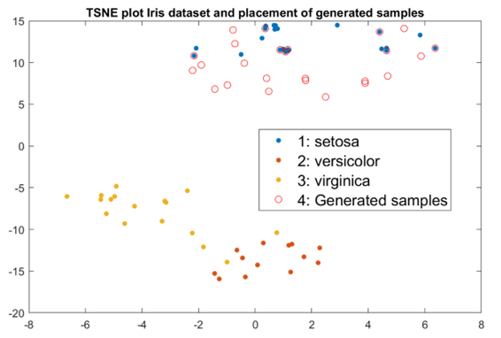
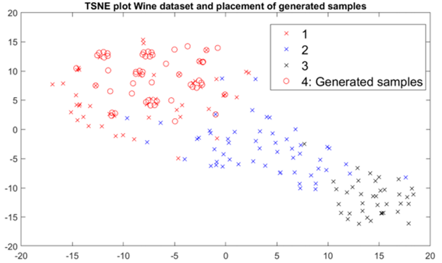
Figure 6: A Normalizing Flow has been trained on the first class for the iris and wine dataset, respectively. The crosses denote the tsne-plot of the training data. The generated examples from sampling the normal distribution are shown in circles.

For the experiments we used as dataset of possible quantum operators the Pauli-($X$, $Y$, $Z$) operations, as well as Hadamard-, cnot-, swap-, phase-shift-, and toffoli-gates. The phase shift gates have a continuous parameter $\theta$ we sampled with $\pi,\frac{\pi}{2},\frac{\pi}{4}$. Thus, only the discrete ordering and selection of quantum gates is optimized by the quantum architecture search. Table 1 summarizes the used datasets, the settings and the train and test splits. Figure 4 summarizes the resulting ROC-Curves and the area-under the ROC-Curve as a final quality measure. Additionally, we provide the ROC-Curves and the obtained results of isolation forests, the local outlier factor (LOF) and the single-class SVM. The final performance is also summarized in table 2. It is apparent that our proposed optimized Quantum Flows can achieve competitive performance. Additionally, the code is available as short and highly performant quantum code. In principle this can easily be implemented on a quantum computer, where we encode a sample into a pure quantum state $|\Psi\rangle$ thats entirely a tensorproduct of computational basis states, apply the quantum circuit and sample the output state, e.g. using tomography. The obtained quantum codes are provided in Figure 5.

Dataset iso-Forest LOF SVM Quantum-NF Iris 1-2 0.93 0.89 1.0 1.0 Iris 2-3 0.88 0.67 0.92 0.97 Wine 1-2 0.946 0.91 0.968 0.97 Wine 2-3 0.92 0.84 0.94 0.95

Table 2: Area under RoC performance on different anomaly detection cases for isolation forests, single-class SVMs and our proposed Quantum Normalizing Flow.

III.4 Normalizing Flow as a generator

As already mentioned in Section 2.2, a Normalizing Flow can be used for several purposes, e.g. anomaly detection as shown in the previous part. Another application is to use the Normalizing Flow as a generator by sampling from the normal distribution and inverting the forward transformation. Thus, in the final experiment, a Normalizing Flow has been trained on the first class of both, the iris and wine dataset, respectively. Afterwards, samples from the normal distribution are generated and transformed using the inverse flow which leads to new samples in the original data. Figure 6 visualizes the tsne-plots for these datasets (in crosses) as well as generated examples (in circles) after sampling complex values from the normal distribution and inverting the learned forward mapping $U$. Note, that the backward transformation can lead to non-useful samples since only the distribution on the absolute values is optimized in the forward flow. Thus, sampling complex numbers can lead to unlikely examples. We therefore verify the samples by backprojecting them onto the normal distribution again and only select samples which have a small KL divergence. As expected, the generated samples are in the domain of the training data and generalize examples among them. Figure 6 shows in crosses the tsne-data for the three classes and in circles the generated samples which are located around the first class label.

IV Summary

In this work, quantum architecture search is used to compute a Normalizing Flow which can be summarized as a bijective mapping from an arbitrary distribution to a normal distribution. The optimization is based on the Kullback-Leibler-divergence. Once such a mapping has been optimized, it can be applied to anomaly detection by comparing the distribution of quantum measurements to the expected normal distribution. In the experiments we perform comparisons to three standard methods, namely isolation forests, the local outlier factor (LOF) and a single-class SVM. The optimized architectures show competitive performance despite being fully implementable on a quantum computer. Additionally we demonstrate how to use the Normalizing Flow as generator by sampling from a normal distribution and inverting the flow.

Acknowledgments

This work was supported, in part, by the Quantum Valley Lower Saxony and under Germany’s Excellence Strategy EXC-2122 PhoenixD. We would like to thank Tobias Osborne (Institute for Theoretical Physics at Leibniz University Hannover) for the fruitful discussions and advice on preparing the manuscript.

References

- [1] M. A. Aizerman, E. A. Braverman, and L. Rozonoer. Theoretical foundations of the potential function method in pattern recognition learning. In Automation and Remote Control,, number 25 in Automation and Remote Control,, pages 821–837, 1964.
- [2] Mennatallah Amer, Markus Goldstein, and Slim Abdennadher. Enhancing one-class support vector machines for unsupervised anomaly detection. In Proceedings of the ACM SIGKDD Workshop on Outlier Detection and Description, ODD ’13, page 8–15, New York, NY, USA, 2013. Association for Computing Machinery.
- [3] Markus M. Breunig, Hans-Peter Kriegel, Raymond T. Ng, and Jörg Sander. Lof: Identifying density-based local outliers. SIGMOD Rec., 29(2):93–104, may 2000.
- [4] Jan Thies̈ Brockmann*, Marco Rudolph*, Bodo Rosenhahn, Bastian Wandt, and (* equal contribution). The voraus-ad dataset for anomaly detection in robot applications. Transactions on Robotics, November 2023.
- [5] Laurent Dinh, Jascha Sohl-Dickstein, and Samy Bengio. Density estimation using Real-NVP. ICLR 2017, 2016.
- [6] Dheeru Dua and Casey Graff. UCI machine learning repository. http://archive.ics.uci.edu/ml, 2017.
- [7] Marina Evangelou and Niall M. Adams. An anomaly detection framework for cyber-security data. Computers & Security, 97:101941, 2020.
- [8] Marco Fanizza, Christoph Hirche, and John Calsamiglia. Ultimate limits for quickest quantum change-point detection. Physical review letters, 131(2):020602, 2023.
- [9] Tharindu Fernando, Simon Denman, David Ahmedt-Aristizabal, Sridha Sridharan, Kristin R. Laurens, Patrick Johnston, and Clinton Fookes. Neural memory plasticity for medical anomaly detection. Neural Networks, 127:67–81, 2020.
- [10] Lukas Franken, Bogdan Georgiev, Sascha Mucke, Moritz Wolter, Raoul Heese, Christian Bauckhage, and Nico Piatkowski. Quantum circuit evolution on nisq devices. In 2022 IEEE Congress on Evolutionary Computation (CEC), pages 1–8, 2022.
- [11] Mathieu Germain, Karol Gregor, Iain Murray, and Hugo Larochelle. Made: Masked autoencoder for distribution estimation. In International Conference on Machine Learning, pages 881–889, 2015.
- [12] Ian Goodfellow, Jean Pouget-Abadie, Mehdi Mirza, Bing Xu, David Warde-Farley, Sherjil Ozair, Aaron Courville, and Yoshua Bengio. Generative adversarial nets. In Advances in neural information processing systems, pages 2672–2680, 2014.
- [13] Sudipto Guha, Nina Mishra, Gourav Roy, and Okke Schrijvers. Robust random cut forest based anomaly detection on streams. In Maria Florina Balcan and Kilian Q. Weinberger, editors, Proceedings of The 33rd International Conference on Machine Learning, volume 48 of Proceedings of Machine Learning Research, pages 2712–2721, New York, New York, USA, 20–22 Jun 2016. PMLR.
- [14] Mingchao Guo, Hailing Liu, Yongmei Li, Wenmin Li, Fei Gao, Sujuan Qin, and Qiaoyan Wen. Quantum algorithms for anomaly detection using amplitude estimation. Physica A: Statistical Mechanics and its Applications, 604:127936, 2022.
- [15] Mingchao Guo, Shijie Pan, Wenmin Li, Fei Gao, Sujuan Qin, XiaoLing Yu, Xuanwen Zhang, and Qiaoyan Wen. Quantum algorithm for unsupervised anomaly detection. Physica A: Statistical Mechanics and its Applications, 625:129018, 2023.
- [16] James A Hanley and Barbara J McNeil. The meaning and use of the area under a receiver operating characteristic (roc) curve. Radiology, 143(1):29–36, 1982.
- [17] Phillip Kaye, Raymond Laflamme, and Michele Mosca. An Introduction to Quantum Computing. Oxford University Press, Inc., USA, 2007.
- [18] Diederik P. Kingma and Max Welling. Auto-encoding variational bayes. CoRR, abs/1312.6114, 2013.
- [19] Durk P Kingma and Prafulla Dhariwal. Glow: Generative flow with invertible 1x1 convolutions. Advances in neural information processing systems, 31, 2018.
- [20] Durk P Kingma, Tim Salimans, Rafal Jozefowicz, Xi Chen, Ilya Sutskever, and Max Welling. Improved variational inference with inverse autoregressive flow. In Advances in neural information processing systems, pages 4743–4751, 2016.
- [21] Ivan Kobyzev, Simon Prince, and Marcus Brubaker. Normalizing flows: An introduction and review of current methods. IEEE Transactions on Pattern Analysis and Machine Intelligence, PP:1–1, 05 2020.
- [22] U. Las Heras, U. Alvarez-Rodriguez, E. Solano, and M. Sanz. Genetic algorithms for digital quantum simulations. Phys. Rev. Lett., 116:230504, Jun 2016.
- [23] Li Li, Minjie Fan, Marc Coram, Patrick Riley, and Stefan Leichenauer. Quantum optimization with a novel gibbs objective function and ansatz architecture search. Phys. Rev. Res., 2:023074, Apr 2020.
- [24] Jin-Min Liang, Shu-Qian Shen, Ming Li, and Lei Li. Quantum anomaly detection with density estimation and multivariate gaussian distribution. Phys. Rev. A, 99:052310, May 2019.
- [25] Fei Tony Liu, Kai Ting, and Zhi-Hua Zhou. On detecting clustered anomalies using sciforest. volume 6322, pages 274–290, 09 2010.
- [26] Fei Tony Liu, Kai Ming Ting, and Zhi-Hua Zhou. Isolation forest. In 2008 Eighth IEEE International Conference on Data Mining, pages 413–422. IEEE, 2008.
- [27] Nana Liu and Patrick Rebentrost. Quantum machine learning for quantum anomaly detection. Phys. Rev. A, 97:042315, Apr 2018.
- [28] Risto Miikkulainen. Neuroevolution, pages 1–8. Springer US, New York, NY, 2020.
- [29] K.G. Murty. Linear Programming. Wiley, 1983.
- [30] H. T. Nguyen and Katrin Franke. A general lp-norm support vector machine via mixed 0-1 programming. In Machine Learning and Data Mining in Pattern Recognition, pages 40–49, Berlin, Heidelberg, 2012. Springer Berlin Heidelberg.
- [31] Michael A Nielsen and Isaac L Chuang. Quantum computation and quantum information. Cambridge university press, 2010.
- [32] George Papamakarios, Theo Pavlakou, and Iain Murray. Masked autoregressive flow for density estimation. Advances in neural information processing systems, 30, 2017.
- [33] W. H. Paul. Logic and Integer Programming. Springer Publishing Company, Incorporated, 1st edition, 2009.
- [34] Rob J. Hyndman Priyanga Dilini Talagala and Kate Smith-Miles. Anomaly detection in high-dimensional data. Journal of Computational and Graphical Statistics, 30(2):360–374, 2021.
- [35] Ali Rahimi and Benjamin Recht. Random features for large-scale kernel machines. In J. Platt, D. Koller, Y. Singer, and S. Roweis, editors, Advances in Neural Information Processing Systems, volume 20. Curran Associates, Inc., 2007.
- [36] Riccardo Rasconi and Angelo Oddi. An innovative genetic algorithm for the quantum circuit compilation problem. Proceedings of the AAAI Conference on Artificial Intelligence, 33:7707–7714, Jul. 2019.
- [37] Shivshankar Reddy, Pranav Poduval, Anand Vir Singh Chauhan, Maneet Singh, Sangam Verma, Karamjit Singh, and Tanmoy Bhowmik. Tegraf: Temporal and graph based fraudulent transaction detection framework. In Proceedings of the Second ACM International Conference on AI in Finance, ICAIF ’21, New York, NY, USA, 2022. Association for Computing Machinery.
- [38] Danilo Rezende and Shakir Mohamed. Variational inference with normalizing flows. In International Conference on Machine Learning, pages 1530–1538. PMLR, 2015.
- [39] Bodo Rosenhahn. Optimization of sparsity-constrained neural networks as a mixed integer linear program. Journal of Optimization Theory and Applications, 199(3):931–954, October 2023. (open access).
- [40] Bodo Rosenhahn and Tobias J. Osborne. Monte carlo graph search for quantum circuit optimization. Phys. Rev. A, 108:062615, Dec 2023.
- [41] Marco Rudolph, Bastian Wandt, and Bodo Rosenhahn. Same same but differnet: Semi-supervised defect detection with normalizing flows. In Winter Conference on Applications of Computer Vision (WACV), January 2021.
- [42] Lukas Ruff, Robert A. Vandermeulen, Nico Görnitz, Alexander Binder, Emmanuel Müller, Klaus-Robert Müller, and Marius Kloft. Deep semi-supervised anomaly detection. In International Conference on Learning Representations, 2020.
- [43] Bernhard Schölkopf, Robert Williamson, Alex Smola, John Shawe-Taylor, and John Platt. Support vector method for novelty detection. In Proceedings of the 12th International Conference on Neural Information Processing Systems, NIPS’99, page 582–588, Cambridge, MA, USA, 1999. MIT Press.
- [44] Clayton Scott and Gilles Blanchard. Novelty detection: Unlabeled data definitely help. In David van Dyk and Max Welling, editors, Proceedings of the Twelth International Conference on Artificial Intelligence and Statistics, volume 5 of Proceedings of Machine Learning Research, pages 464–471, Hilton Clearwater Beach Resort, Clearwater Beach, Florida USA, 16–18 Apr 2009. PMLR.
- [45] Peter Selinger. Towards a quantum programming language. Mathematical Structures in Computer Science, 14(4):527–586, August 2004.
- [46] Gael Sentís, John Calsamiglia, and Ramon Muñoz Tapia. Exact identification of a quantum change point. Phys. Rev. Lett., 119:140506, Oct 2017.
- [47] Gael Sentís, Esteban Martínez-Vargas, and Ramon Muñoz Tapia. Online strategies for exactly identifying a quantum change point. Phys. Rev. A, 98:052305, Nov 2018.
- [48] Tom Wehrbein, Marco Rudolph, Bodo Rosenhahn, and Bastian Wandt. Probabilistic monocular 3D human pose estimation with normalizing flows. Proceedings of the IEEE International Conference on Computer Vision, 2021.
- [49] Sirui Xie, Hehui Zheng, Chunxiao Liu, and Liang Lin. SNAS: stochastic neural architecture search. In International Conference on Learning Representations, 2019.
- [50] Shi-Xin Zhang, Chang-Yu Hsieh, Shengyu Zhang, and Hong Yao. Neural predictor based quantum architecture search. Machine Learning: Science and Technology, 2(4):045027, oct 2021.
- [51] Weiwei Zhu, Jiangtao Pi, and Qiuyuan Peng. A brief survey of quantum architecture search. In Proceedings of the 6th International Conference on Algorithms, Computing and Systems, ICACS ’22, New York, NY, USA, 2023. Association for Computing Machinery.