Dynamic Sparse Learning: A Novel Paradigm for
Efficient Recommendation

Abstract.

In the realm of deep learning-based recommendation systems, the increasing computational demands, driven by the growing number of users and items, pose a significant challenge to practical deployment. This challenge is primarily twofold: reducing the model size while effectively learning user and item representations for efficient recommendations. Despite considerable advancements in model compression and architecture search, prevalent approaches face notable constraints. These include substantial additional computational costs from pre-training/re-training in model compression and an extensive search space in architecture design. Additionally, managing complexity and adhering to memory constraints is problematic, especially in scenarios with strict time or space limitations. Addressing these issues, this paper introduces a novel learning paradigm, Dynamic Sparse Learning (DSL), tailored for recommendation models. DSL innovatively trains a lightweight sparse model from scratch, periodically evaluating and dynamically adjusting each weight’s significance and the model’s sparsity distribution during the training. This approach ensures a consistent and minimal parameter budget throughout the full learning lifecycle, paving the way for “end-to-end” efficiency from training to inference. Our extensive experimental results underline DSL’s effectiveness, significantly reducing training and inference costs while delivering comparable recommendation performance. We give an code link of our work: https://github.com/shuyao-wang/DSL.

1. Introduction

Recommendation systems (Zheng et al., 2022b; Wang et al., 2020, 2021) provide personalized services for today’s web and have achieved significant success in various fields, such as e-commerce platforms, medical care (Zheng et al., 2022a, 2023c, 2021), education (Zheng et al., 2023b) and job search (Zheng et al., 2023a). At its core is learning high-quality representations for users and items based on historical interaction data. The rapidly growing population of users and items on one hand promotes the demands for large-scale recommender systems (Wu et al., 2023), while on the other hand posing great challenges for model training and inference, such as unaffordable memory overheads, computational costs, and inference latency. Hence, efficient recommendation, i.e., lightweight model, with low costs of training and inference, is of great need and significance.

Table 1. Comprehensive comparisons with existing efficient recommendation methods.

Method	Category	Saving			End-to-end	Budget controllable	Non-uniform embedding size	Performance reserved
		Training cost	Inference cost	Memory
TKD (Kang et al., 2021)	KD	✗	✓	✗	✗	✓	✗	✗
RKD (Tang and Wang, 2018)	KD	✗	✓	✗	✗	✓	✗	✗
AutoEmb (Zhao et al., 2021a)	AutoML	✗	✓	✗	✓	✗	✓	✓
ESAPN (Liu et al., 2020)	AutoML	✗	✓	✗	✓	✗	✓	✓
PEP (Liu et al., 2021)	MP	✓	✓	✓	✓	✗	✓	✗
LTH-MRS (Wang et al., 2022)	MP	✗	✓	✗	✗	✗	✓	✓
Ours	MP	✓	✓	✓	✓	✓	✓	✓

Various solutions have been proposed for efficient recommendation, which can be categorized into the following three research lines, each of which has inherent limitations.

• Knowledge Distillation (KD) (Gou et al., 2021; Kweon et al., 2021; Yang et al., 2022; Tao et al., 2022; Lee and Kim, 2021; Kang et al., 2021, 2022) distills knowledge from a pre-trained large-scale model (i.e., teacher model) to a compact model (i.e., student model) for efficient inference. On the one hand, the proceeds of KD mainly lie in the reduction of inference costs by using the lightweight student model. Yet, it still needs to train a cumbersome teacher model from scratch, leaving the overall training cost not reduced. On the other hand, the knowledge of the teacher models often cannot thoroughly transfer to the student models (Tang and Wang, 2018), usually incurring a large performance degradation (Kang et al., 2021; Kweon et al., 2021).

• Automated Machine Learning (AutoML) (Chen et al., 2022d; Zheng et al., 2022c; Liu et al., 2021; Zhao et al., 2021b, a; Liu et al., 2020) aims to search lightweight model architectures in a given search space via diverse strategies, including gradient-based optimization (Ruder, 2016; Liu et al., 2018), reinforcement learning (Liu et al., 2021) , or evolutionary algorithms (Qin et al., 2008). However, the search space should be manually predefined with human prior knowledge (Chen et al., 2022d). In addition, the complex procedures of optimization and performance estimation (Chen et al., 2022d) also lead to an unaffordable computational cost.

• Model Pruning (MP) (Frankle and Carbin, 2018; Han et al., 2015; Zhu and Gupta, 2018; Tanaka et al., 2020; Wang et al., 2022) trims down the model size by removing redundant parameters from the full model. It aims to find a sparse and lightweight model that can best retain the performance of the full model. However, it needs to empirically find intriguing sparse embedding tables by an iterative “train-prune-retrain” pipeline (Frankle and Carbin, 2018; Wang et al., 2022), which still suffers from the expensiveness of the post-training pruning.

We present a clear summary of several representative efforts and their respective properties in Table 1. Further discussions can be found in Section 5. Scrutinizing the limitations of these solutions, they either require model pre-training or complex optimization processes of architecture search. Hence, the benefits mainly come from the inference stage, while greatly increasing the training workload.

In view of that, we aim to design a simple and lightweight learning paradigm for recommendation models that can simultaneously trim down the training and inference costs, with comparable performance. By inspecting the design of the conventional models, we find that most of them impose a constraint on the length of representations during model training, that is, embedding each user or item as a dense vector with a preset dimension (aka., embedding table). However, in expectation, a flexible model is capable of assigning different embedding sizes to diverse users or items based on the information they carry. Intuitively, users having multiple interests (or items attracting diverse audiences) should be more informative than the inactive counterparts, and hence should be represented with larger dimensions, and vice versa (Liu et al., 2020; Zhao et al., 2021a; Chen et al., 2023). Hence, there may exist a large number of redundant weights in the full embedding table, resulting in an over-parameterized model, which greatly hinders efficiency. Then a question raises naturally: “Can we relax the limitation on the embedding size of the model, and let the model automatically remove or add weights to achieve a dynamic embedding size during training?”

Towards this end, we propose an end-to-end learning paradigm for recommendation: Dynamic Sparse Learning (DSL). Specifically, given a randomly initialized model, DSL first randomly prunes the model to a predefined budget and trains the sparse model. During the training process, it periodically adjusts the sparsity distribution of the model parameters via two dynamic strategies: pruning and growth. The implemented pruning strategy identifies and eliminates weights that have negligible impact on the performance, thereby effectively reducing redundancy in the model parameters. While the growth process explores the potential informative weights that can improve the performance, thereby reactivating important parameters. DSL sticks to a fixed and small budget by maintaining the same ratio of pruning and growth throughout the whole training stage, thus effectively reducing both the training and inference complexity. DSL is a model-agnostic and plug-and-play learning framework that can be applied to various models. In contrast to existing efforts in Table 1, it achieves the attractive prospect of “end-to-end” efficiency from training to inference. We implement DSL on diverse collaborative recommendation models, and conduct extensive experiments on benchmark datasets. Experimental results show that DSL can effectively trim down both the training and inference costs, with comparable performance.

Overall, we make the following contributions:

• Problem: We argue that large-scale recommendation models usually suffer from high training and inference complexity. Unfortunately, most solutions mainly alleviate the computational cost of inference, but double the cost of model training.

• Algorithm: We propose an efficient learning paradigm for recommendation, named DSL. It trains lightweight sparse models and sticks to a fixed parameter budget during the whole training stage. Hence, it can achieve end-to-end efficiency from training to inference.

• Experiments: We conduct extensive experiments on diverse recommendation models. The results demonstrate the superiority and effectiveness of DSL. More visualizations with in-depth analyses demonstrate the rationality of DSL.

2. Preliminaries

2.1. Notations

This paper focuses on collaborative recommendation settings. Given a recommender system with $N$ users and $M$ items, we define the set of users $\mathcal{U}=\left\{u\right\}$, items $\mathcal{I}=\{i\}$, and their interactions $\mathcal{{O}}={\left\{y_{ui}\right\}}$, where $y_{ui}=1$ denotes user $u$ has adopted item $i$ before, otherwise $y_{ui}=0$. For convenience, we organize them as a graph $\mathcal{G}=\left\{\mathcal{V},\mathcal{E}\right\}$. where $\mathcal{V}=\left\{v_{1},\cdots,v_{N+M}\right\}$ is the node set comprising both user and item nodes, $\mathcal{E}=\left\{(u,i)|u\in\mathcal{U},i\in\mathcal{I},y_{ui}=1\right\}$ is the edge set containing all observed interactions between users and items. Each node is encoded into a $d$-dimensional embedding vector $\mathbf{e}\in\mathbbm{R}^{d}$. We define $f$ as the recommendation model, and the embedding table of $f$ can be represented as follow:

(1) $$\mathbf{E}=[\underbrace{\mathbf{e}_{u_{1}},\mathbf{e}_{u_{2}},\cdots,\mathbf{e}_{u_{N}}}_{\text{users}};\underbrace{\mathbf{e}_{i_{1}},\mathbf{e}_{i_{2}},\cdots,\mathbf{e}_{i_{M}}}_{\text{items}}]^{\top}\in\mathbb{R}^{(N+M)\times d}.$$

For a given recommendation model $f$, it’s observable that the parameters of the embedding table expand linearly with the number of users and items. In collaborative recommendation, popular models like NeuMF (He et al., 2017) and LightGCN (He et al., 2020) primarily rely on learning the embedding table. Though other learnable parameters in $f$ may impact the final computational cost, this paper primarily considers the cost associated with embeddings.

2.2. Efficient Recommendation

2.2.1. Problem Formulation.

The efficient recommendation aims to conserve resources while maintaining the recommendation quality. These resources often encompass computational costs during training and testing, memory space, and latency time, all crucial for practical applications. We now formally define the problem of efficient recommendation.

Problem 1 (Efficient Recommendation).

Given a well-trained recommendation model $f$ that attains performance level $P$, which requires resources $C_{\rm tr}$, $C_{\rm te}$ and $C_{\rm m}$ for training, testing, and memory cost, respectively. Consider another model $f^{\prime}$ that achieves performance level $P^{\prime}$ after convergence with $C_{\rm tr}^{\prime}$, $C_{\rm te}^{\prime}$ and $C_{\rm m}^{\prime}$. The task of efficient recommendation is to find the alternative $f^{\prime}$ that is capable of replacing $f$, satisfying: $C_{\rm tr}^{\prime}<C_{\rm tr}$, $C_{\rm te}^{\prime}<C_{\rm te}$, $C_{\rm m}^{\prime}<C_{\rm m}$ and $P^{\prime}\approx P$.

The objective of Problem 1 is to look for a model with fewer parameters to conserve resources. We summarize and discuss existing methods towards this goal from two perspectives: coarse-grained model architectures and fine-grained model architectures.

2.2.2. Efficiency via Coarse-grained Model Architectures.

The efficiency of the model is influenced by its coarse-grained architecture, which is determined by the dimensions of the embedding table. Reducing the dimension of the embedding table can enhance efficiency for model training and inference. However, these streamlined models often struggle to deliver the promising performance equivalent to their larger counterparts, i.e., $P^{\prime}\approx P$ in Problem 1 does not hold. To address this issue, knowledge distillation (KD) methods are employed (Tang and Wang, 2018; Kang et al., 2021; Kweon et al., 2021), which distills knowledge from larger pre-trained teacher models into smaller ones to improve the recommendation performance. However, extensive studies (Kweon et al., 2021) demonstrate that there still exists a non-negligible performance gap between small and large models. Furthermore, the computational expense of pre-training is not mitigated, rendering these approaches insufficient for fully resolving Problem 1.

2.2.3. Efficiency via Fine-grained Model Architectures.

Approaches from a microscopic perspective assign distinct embedding dimensions to individual users and items, presenting a fine-grained model design philosophy to achieve efficiency. AutoML-based methods (Zheng et al., 2022c; Chen et al., 2022d) search for the optimal model architecture within a predefined search space. However, perfectly defining the search space is challenging (Zheng et al., 2022c). Furthermore, complex procedures of optimization and performance estimation (Chen et al., 2022d) also double the cost, making it difficult to solve Problem 1. Another research line is model pruning, guided by the lottery ticket hypothesis (LTH) (Frankle and Carbin, 2018; Chen et al., 2020b; Sui et al., 2023a). It states that sparse models discovered by pruning can replace full models without performance degradation. Despite its potential benefits, LTH has not been extensively studied in the field of recommender systems. In this regard, we provide a formal definition of the winning ticket in recommendation.

Definition 0 (Winning Ticket).

Given a recommendation model $f$ with embedding table $\mathbf{E}$, a binary mask $\mathbf{M}\in\left\{0,1\right\}^{{\|\mathbf{E}\|}_{0}}$ can create a sparse embedding table: $\mathbf{E}^{\prime}\leftarrow\mathbf{M}\odot\mathbf{E}$, where $\odot$ denotes the element-wise product.

1. The model $f(\mathcal{G},\mathbf{E})$ with a dense embedding table $\mathbf{E}$ can obtain the performance $P$ after training $T$ iterations.

2. A sparse model $f(\mathcal{G},\mathbf{E}^{\prime})$ can obtain the performance level $P^{\prime}$ after training $T^{\prime}$ iterations.

If $\exists\,\mathbf{M}\in\left\{0,1\right\}^{{\|\mathbf{E}\|}_{0}}$ such that $T^{\prime}\leq T$, $P^{\prime}\geq P$ and ${{\|\mathbf{E}^{\prime}\|}_{0}}\ll{{\|\mathbf{E}\|}_{0}}$, then we define the sparse model $\mathbf{E}^{\prime}$ as a winning ticket.

As per Definition 1, winning tickets present a natural solution to Problem 1, which possesses an attractive property: we could have trained from a sparse lightweight model if only we had known which mask to choose. Recent work LTH-MRS (Wang et al., 2022) has explored and validated the existence of lottery tickets in recommendation models. However, it adopts a similar pruning strategy as in LTH (Frankle and Carbin, 2018) — iterative magnitude pruning — to locate the winning tickets. This multiple-round training strategy is a surefire way to find the winning ticket, while it will largely increase the training costs. Although winning tickets are fascinating, how to efficiently find them is still an open problem (You et al., 2019; Evci et al., 2022). We summarize some specific studies of efficient recommendation in Table 1. More discussions are provided in Section 5.

3. Methodology

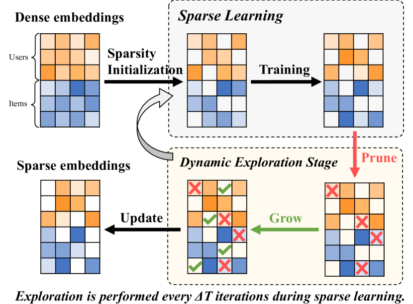
Figure 1. The overview of the proposed Dynamic Sparse Learning (DSL) framework.

3.1. Dynamic Sparse Learning

In conventional model learning, all users and items are represented by embeddings of uniform size. However, since the amount of information carried by diverse users and items is very likely to be different, the strategy of assigning the same embedding size may be suboptimal. Observations from prior studies such as ESAPN (Liu et al., 2020), UnKD (Chen et al., 2023), and LTH-MRS (Wang et al., 2022), suggest that inactive users and unpopular items may contain less information, necessitating smaller embedding sizes to depict their simpler characteristics. Hence, we relax the constraint on embedding size and encourage the model to dynamically discover those redundant weights during learning. The overview of DSL is displayed in Figure 1, which includes three steps: sparsity initialization, sparse learning, and dynamic exploration. DSL initiates the training process with a randomly sparsified model. Furthermore, the dynamic exploration step is periodically (i.e., $\Delta{T}$ training iterations) introduced during the sparse learning process. Now we elaborate on these three steps in detail.

3.1.1. Sparsity Initialization

Given a dense user-item embedding table $\mathbf{E}$, we first establish the model’s sparsity $s\in(0,1)$. Then we initialize a binary mask $\mathbf{M}\in\left\{0,1\right\}^{{\|\mathbf{E}\|}_{0}}$ with a random sparsity distribution, where ${{\|\mathbf{M}\|}_{0}}={{\|\mathbf{E}\|}_{0}}\cdot(1-s)$, and we can obtain a sparse embedding table $\mathbf{E}^{\prime}\leftarrow\mathbf{M}\odot\mathbf{E}$. Please note that the binary mask is solely introduced to aid in the description of our operations. In practice, there is no need to store this additional matrix. To ensure a constant model parameter budget, we fix the sparsity $s$ throughout the whole training process.

3.1.2. Sparse Learning

We directly train the sparse model until entering the next dynamic exploration stage. As shown in Figure 1, we will transition between the exploration stage and the sparse learning multiple times. Since a new sparse distribution, i.e., model architecture, is obtained after each dynamic exploration, the model needs to retune parameters to fit new architecture. We define $T_{end}$ as the total training iterations and $\Delta{T}$ as the number of iterations for each round of the sparse learning. We find that both too-large and too-small values of $\Delta{T}$ can greatly deteriorate the performance. Given a fixed training iteration ${T_{end}}$, if we make $\Delta{T}$ too large, it will greatly reduce the number of times entering the exploration step, which means that the model has fewer opportunities to modify the current model structure. Ultimately, when $\Delta{T}\to\infty$, it is equivalent to directly training a randomly pruned model, which will lead to poor performance. When $\Delta{T}$ is too small, the model cannot adequately adjust the parameters to adapt to the current architecture, so when entering the exploration stage, it is difficult to accurately remove redundant weights or add important weights. This will undoubtedly degrade the performance. Hence, an appropriate number of sparse training iterations $\Delta{T}$ is necessary. In view of that, we conduct comprehensive ablation studies in Section 4.4.1.

Algorithm 1 Dynamic Sparse Learning

1:Dense embedding table $\mathbf{E}$, Dataset $\mathcal{D}$, Random binary mask $\mathbf{M}\in\left\{0,1\right\}^{{\|\mathbf{E}\|}_{0}}$ with sparsity $s$, Loss $\mathcal{L}$, Learning rate $\eta$, Initial update ratio $\rho_{0}$, $\Delta{T}$, $T_{end}$.

2:Initialize sparse table $\mathbf{E}\leftarrow\mathbf{M}\odot\mathbf{E}$

3:for training iteration $t\in\{1,...,T_{end}\}$ do

4:     Sampling a batch $b_{t}\sim\mathcal{D}$

5:     if $(t\ {\rm mod}\ {\Delta{T}}==0)$ then

6:         $\rho_{t}\leftarrow{\rm CosineAnnealing}(\rho_{0},t,T_{end})$

7:         Creating $\mathbf{M}$ by pruning and growth with $\rho_{t}$

8:         Updating sparse embedding table $\mathbf{E}$

9:     else

10:    $\mathbf{E}\leftarrow\mathbf{E}-{\eta}{\nabla_{\mathbf{E}}}{\mathcal{L}}$

11:     end if

12:end for

13:return A sparse embedding table

3.1.3. Dynamic Exploration

Exploration is performed every $\Delta{T}$ iteration during the model training process. In this step, we dynamically adjust the sparsity distribution of the model parameters. There exist three key components: update schedule, pruning principle, and growth principle.

• Update schedule. To ensure the stability of the exploration stage, we set the update ratio $\rho_{t}$ for every exploration using a cosine annealing schedule, where $t$ is the current training step. Take $\rho_{0}$ as the initial update ratio at the 0-th iteration. Following (Loshchilov and Hutter, 2016), the decay function is defined as:

  (2) $${\rho_{t}}=\frac{\rho_{0}}{2}\left(1+{\rm cos}\left(\frac{\pi t}{T_{\text{end }}}\right)\right).$$

  As model training approaches convergence, the update ratio should gradually decrease to ensure stable convergence. Hence, this decay strategy facilitates the gradual adoption of the model architecture to stabilize the training process. We also verify the effectiveness of this strategy in Section 4.4.3.

• Pruning principle. Following (Frankle and Carbin, 2018), we adopt the weight magnitude as the pruning indicator. We prune a $\rho_{t}$ ratio of the lowest-magnitude weights. It is worth mentioning that we maintain the same update ratio in both the pruning and growth process to stick to a fixed budget.

• Growth principle. We monitor the gradients of the pruned weights to assess their potential importance in the final prediction. Then we reactivate a $\rho_{t}$ ratio of the pruned weights having the highest gradient magnitudes, which will participate in the next round of sparse learning. Such a growth principle provides a regret mechanism for pruning, serving as compensation for the information loss caused by the previous greedy pruning (Wang et al., 2022).

The overview of the proposed framework is depicted in Figure 1, and the detailed pipeline of DSL is summarized in Algorithm 1.

3.2. Technique Analysis

In this section, we provide detailed analyses and discussions of the working mechanism of the DSL. It can achieve sparse learning while retaining the performance for the following reasons:

• Dynamic Architecture Exploration. Recklessly training a static model architecture with random sparsity distribution often leads to suboptimal performance (Wang et al., 2022). This is mainly due to the existence of poor natural model architectures (Liu et al., 2018), which result in subpar performance. In contrast, DSL flexibly adjusts the suboptimal structure during training, allowing the model to dynamically learn the importance of weights, thus achieving better performance.

• Sufficient Sparse Learning. DSL monitors the states of the parameters, such as magnitudes or gradients, which reflect their importance. This provides a guarantee for the subsequent precise parameter pruning and growth process. However, it will also lead to insufficient exploration, resulting in a trade-off between the number of exploration cycles and sparse learning iterations. In Section 4.4, we conduct extensive experiments to verify this.

• Sufficient Exploration Space. One key strength of DSL is its ability to reactivate important parameters that were pruned, thus avoiding the problem of degraded performance in compressed models. Furthermore, as DSL searches for the most critical pruned parameters to reactivate in each round, DSL has the potential to surpass the original model’s performance (cf. Section 4.3). Additionally, the regret mechanism imbues DSL with more flexibility in adapting to different model architectures, thus enhancing the stability of the compressed model.

3.3. Complexity Analysis

We use LightGCN (He et al., 2020), a widely used collaborative recommendation model, to instantiate this. It contains two critical components: light graph convolution (LGC) and layer combination (LC). Assuming that it performs $L$-layer LGC with the adjacency matrix $\mathbf{A}$ of graph $\mathcal{G}$. Then the time complexity of LGC is $\mathcal{O}\left(\|\mathbf{A}\|_{0}\times d\times L\right)$; LC is $\mathcal{O}\left(N\times d+M\times d\right)$ and similarity computation is $\mathcal{O}\left(N\times M\times d\right)$. Due to $(N+M)\ll(N\times M)$, the total time complexity is approximated to $\mathcal{O}\left((\|\mathbf{A}\|_{0}\times L+N\times M)\times d\right)$. For the sparse model with sparsity $s$, the time complexity will be greatly reduced to $\mathcal{O}\left((\|\mathbf{A}\|_{0}\times L+N\times M)\times d\times(1-s)\right)$.

4. Experiments

Table 2. Performance over diverse models. $l$ and $d$ denote the layer number and the embedding size, respectively. Following work (Chen et al., 2021a), we use MACs (Tr.) and MACs (In.) to measure the training and inference computational costs, respectively.

Model	MovieLens-1M				CiteUlike				Foursquare
	MACs (Tr.)	MACs (In.)	Recall/HR	NDCG	MACs (Tr.)	MACs (In.)	Recall/HR	NDCG	MACs (Tr.)	MACs (In.)	Recall/HR	NDCG
NeuMF	3.13e+13	9.68e+08	0.7867	0.4478	3.85e+12	8.87e+08	0.4000	0.2053	3.72e+13	2.50e+09	0.4940	0.2723
+ DSL	2.09e+13	6.47e+08	0.7525	0.4531	2.58e+12	5.93e+08	0.4000	0.2809	2.49e+13	1.67e+09	0.5663	0.3449
ConvNCF	1.50e+15	4.65e+10	0.7745	0.5261	1.83e+14	4.26e+10	0.3429	0.2816	1.76e+15	1.20e+11	0.5301	0.2583
+ DSL	0.38e+15	1.19e+10	0.7990	0.4875	0.46e+14	1.09e+10	0.3714	0.2076	0.45e+15	0.31e+11	0.4940	0.3115
MultVAE	2.40e+12	1.08e+10	0.3099	0.3052	1.36e+13	6.40e+10	0.2260	0.1278	4.61e+13	2.24e+11	0.1550	0.1639
+ DSL	1.20e+12	0.54e+10	0.3080	0.3005	0.68e+13	3.20e+10	0.2044	0.1093	3.69e+13	1.79e+11	0.1427	0.1485
CDAE	2.67e+11	1.26e+10	0.3254	0.3236	3.60e+12	6.77e+10	0.1687	0.1080	1.15e+13	2.27e+11	0.2504	0.2452
+ DSL	1.33e+11	0.63e+10	0.3657	0.3656	1.80e+12	3.39e+10	0.1423	0.0962	0.92e+13	1.82e+11	0.2350	0.2303
	Amazon-Book				Yelp2018				Gowalla
	MACs (Tr.)	MACs (In.)	Recall	NDCG	MACs (Tr.)	MACs (In.)	Recall	NDCG	MACs (Tr.)	MACs (In.)	Recall	NDCG
LightGCN ($l$=3)	1.59e+20	6.88e+13	0.0414	0.0321	4.00e+19	3.32e+13	0.0642	0.0528	1.75e+19	2.21e+13	0.1816	0.1550
+ DSL	0.95e+20	4.14e+13	0.0416	0.0325	2.67e+19	2.22e+13	0.0641	0.0527	1.16e+19	1.48e+13	0.1813	0.1547
LightGCN ($l$=4)	2.12e+20	9.17e+13	0.0406	0.0313	5.34e+19	4.42e+13	0.0649	0.0530	2.33e+19	2.95e+13	0.1830	0.1550
+ DSL	1.17e+20	5.06e+13	0.0405	0.0314	3.34e+19	2.77e+13	0.0651	0.0536	1.45e+19	1.84e+13	0.1821	0.1544
UltraGCN ($d$=64)	5.02e+13	6.24e+11	0.0678	0.0553	2.37e+13	15.5e+10	0.0673	0.0554	9.05e+13	1.61e+11	0.1858	0.1576
+ DSL	2.69e+13	1.56e+11	0.0685	0.0563	1.68e+13	9.89e+10	0.0645	0.0530	6.23e+13	1.03e+11	0.1742	0.1448
UltraGCN ($d$=128)	9.85e+13	1.25e+12	0.0712	0.0582	4.62e+13	3.09e+11	0.0676	0.0556	1.76e+14	3.22e+11	0.1844	0.1539
+ DSL	5.18e+13	0.31e+12	0.0727	0.0582	3.23e+13	1.98e+11	0.0651	0.0532	1.20e+14	2.06e+11	0.1792	0.1478

To verify the superiority of DSL, we conduct extensive experiments to answer the following Research Questions:

• RQ1: How does DSL perform in terms of cost and performance, when applying to diverse recommendation models?

• RQ2: Compared with the state-of-the-art solutions for efficient recommendation, how does DSL perform?

• RQ3: For different hyper-parameters in DSL, what are their roles or impacts on performance?

• RQ4: Does DSL explore the model architectures with regular patterns or insightful interpretations?

4.1. Experimental Setup

4.1.1. Datasets & Metrics.

We conduct experiments on 6 benchmark datasets, including 3 small-scale datasets: MovieLens-1M, CiteUlike and Foursquare, and 3 large-scale datasets: Amazon-Book, Yelp2018 and Gowalla. According to problem definition 1, we need to evaluate our method from the following two perspectives. In terms of model performance, we adopt the full-ranking protocol (He et al., 2020) and present the results using the widely used Recall@20, HR@20, and NDCG@20 metrics. In terms of costs, following most pruning-related studies (Chen et al., 2022c), we adopt the Training MACs (Tr.), Inference MACs (In.), and Memory to evaluate the computational efficiency and memory overhead.

4.1.2. Backbone Models.

To verify that DSL can be applied to diverse models, we choose 6 backbone models, which can be divided into the following three categories:

• Collaborative filtering models: NeuMF (He et al., 2017), ConvNCF (He et al., 2018).

• Autoencoder-based models: CDAE (Wu et al., 2016), MultVAE (Liang et al., 2018).

• Graph-based models: LightGCN (He et al., 2020), UltraGCN (Mao et al., 2021).

4.1.3. Baselines.

To demonstrate the superiority of DSL, we compare it with diverse state-of-the-art solutions for efficient recommendation. They fall into the following three categories:

• KD-based methods: TKD (Kang et al., 2021), RKD (Tang and Wang, 2018).

• AutoML-based methods: AutoEmb (Zhao et al., 2021a), ESAPN (Liu et al., 2020).

• MP-based methods: PEP (Liu et al., 2021), LTH-MRS (Wang et al., 2022), Random Pruning (RP) (Zhu and Gupta, 2018), One-shot Magnitude Pruning (OMP) (Han et al., 2015), Without Rewinding (WR) (Savarese et al., 2020).

4.2. Performance Evaluations (RQ1)

We implement DSL on various models, with settings detailed in the code link. The results presented in Table 2 highlight the achievement of extreme sparsity levels — the highest degree of sparsity attainable without incurring significant performance loss. From these results, we make the following Observations:

Obs1: DSL consistently reduces both training and inference costs on diverse models with comparable performance. DSL is first applied to four backbone models, i.e., CF-based and autoencoder-based models, using three small-scale datasets (refer to the first four rows). Specifically, with NeuMF and ConvNCF, the computational costs of training and testing are reduced by approximately 50.0% $\sim$ 74.4%. For autoencoder-based models, MultVAE and CDAE, the training and inference MACs are cut by about 20% $\sim$ 50%. These findings underline the effectiveness of DSL with classic models and smaller datasets. Next, DSL is deployed on two widely used graph-based models of different layer depths and embedding sizes, and tested on three large-scale datasets. For LightGCN with different layers and UltraGCN with different embedding sizes, DSL achieves 29.3%$\sim$47.4% training MACs saving and 33.2%$\sim$75.0% inference MACs saving. These findings confirm the efficacy of DSL in reducing both training and inference costs across diverse models and datasets without significant performance compromise. Moreover, DSL outperforms the full model in some cases, such as NeuMF on MovieLens-1M and CiteUlike, and UltraGCN on the Amazon-Book. This suggests DSL’s ability to prune redundant weights and explore more meaningful model architectures.

Table 3. Result comparisons of diverse solutions for efficient recommendation. The average and standard deviation results are reported across five random runs. We adopt the models with different embedding sizes. The bold and underlined numbers highlight the best and the second best performance, respectively.

Category	Method	Embedding size=64				Embedding size=128				Average MACs
		MACs (Tr.)	Memory	Recall	NDCG	MACs (Tr.)	Memory	Recall	NDCG
	Baseline	4.00e+19	2103M	0.0642(.0001)	0.0528(.0002)	8.01e+19	2399M	0.0673(.0003)	0.0550(.0001)	0
KD	RKD	6.00e+19	2103M	0.0558(.0005)	0.0460(.0004)	1.20e+20	2399M	0.0610(.0003)	0.0493(.0004)	+ 49.9%
	TKD	6.67e+19	2103M	0.0615(.0007)	0.0514(.0006)	1.34e+20	2399M	0.0645(.0005)	0.0533(.0003)	+ 67.1%
AutoML	AutoEmb	7.92e+19	4210M	0.0627(.0002)	0.0511(.0003)	1.58e+20	4521M	0.0654(.0003)	0.0536(.0003)	+ 97.7%
	ESAPN	1.91e+20	4364M	0.0638(.0002)	0.0525(.0002)	3.81e+20	4675M	0.0672(.0003)	0.0545(.0002)	+ 376.6%
MP	RP	2.67e+19	1052M	0.0557(.0011)	0.0458(.0010)	5.34e+19	1199M	0.0608(.0009)	0.0498(.0009)	- 33.3%
	OMP	6.67e+19	2103M	0.0622(.0000)	0.0509(.0001)	1.33e+20	2399M	0.0661(.0001)	0.0542(.0000)	+ 66.4%
	WR	1.93e+20	2103M	0.0621(.0003)	0.0501(.0004)	3.85e+20	2399M	0.0661(.0004)	0.0537(.0005)	+ 381.6%
	PEP	3.34e+19	2082M	0.0592(.0013)	0.0484(.0011)	6.68e+19	2375M	0.0623(.0009)	0.0501(.0010)	- 16.5%
	LTH-MRS	1.93e+20	2103M	0.0635(.0000)	0.0525(.0001)	3.85e+20	2399M	0.0666(.0001)	0.0545(.0001)	+ 381.6%
	DSL (Ours)	2.67e+19	1052M	0.0641(.0002)	0.0527(.0001)	5.34e+19	1199M	0.0675(.0003)	0.0553(.0002)	- 33.3%

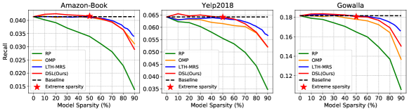
Figure 2. Performance comparisons with different sparsity levels. The star denotes the extreme sparsity of DSL, which achieves the similar performance levels as the baseline.

4.3. Comparisons with Baselines (RQ2)

We compare DSL with other baselines using LightGCN as backbone model, analyzing its performance across diverse embedding sizes. To ensure fairness, we commence by utilizing identical dense models and maintaining equivalent compression ratios. Specifically, we implement a 50% sparsity level for pruning-based methods, whereas for KD-based methods, the size of the student models is half that of their corresponding teacher models, i.e., the original dense models. The experimental results are shown in Table 3, we make the following observations:

Obs2: Both KD-based and AutoML-based methods suffer from large training costs. For KD-based methods, the performance of RKD and TKD dropped on average by 11.22% and 4.34%, respectively. Furthermore, they all require large-scale pre-trained teacher models, which greatly increases the training costs. For RKD and TKD, the training MACs increase on average by 49.9% and 67.1%, respectively. For AutoML-based methods, we can observe that both AutoEmb and ESAPN can keep comparable performance with baseline. However, they also involve additional parameters, such as a controller or policy networks, and experience complex optimization processes. It inevitably results in large training computational and memory costs. In contrast, our proposed DSL dynamically trains sparse and lightweight models. On the one hand, its dynamic exploration stage can find suitable model architectures, thus guaranteeing comparable performance. On the other hand, the sparse models and end-to-end training strategy guarantee low training computational costs and memory overhead.

Obs3: DSL consistently outperforms other pruning-based methods. PEP achieves smaller training costs due to its dynamic training process. However, the performance drops by 6.84%$\sim$9.03% compared to the baseline, since the dynamic pruning thresholds will lead to unstable training. OMP has relatively good performance, while it needs one-shot pruning on pre-trained models. In contrast, LTH-WRS outperforms OMP. The pruning ratio in each round is much smaller than OMP, so redundant weights can be pruned more accurately. Unfortunately, the iterative ”train-prune-retain” pipeline incurs significant training costs amounting to approximately 380% increase in comparison to the baseline. Moreover, while RP delivers comparable memory and training costs to DSL, its performance deteriorates by 9.66%$\sim$13.24%. This is attributed to RP’s use of solely static sparse models during training, without incorporating DSL’s exploratory stage. Finally, we can easily observe that our proposed DSL can overcome all the shortcomings of the above pruning methods. It effectively saves training and memory costs with comparable performance.

Obs4: DSL can achieve better “performance-sparsity” trade-offs. To explore the relationships between performance and the model sparsity, we plot “performance-sparsity” curve from 0$\sim$90% sparsity levels. The results are depicted in Figure 2. We can observe that the performance of RP drops sharply with increasing sparsity. OMP performs worse than DSL, while LTH-MRS achieves comparable performance with DSL. We also observe that DSL even outperforms baseline in some cases, such as 10%$\sim$40% sparsity levels on Amazon-Book and 0$\sim$40% sparsity levels on Yelp2018. It demonstrates that the DSL can discover better model structures than the baselines through dynamic explorations. These results further demonstrate that our proposed DSL can achieve better trade-offs while keeping lower computational costs.

4.4. Ablation Study (RQ3)

4.4.1. Effect of Update Interval.

To explore the effect of update intervals, we adjust ${\Delta T}$ under different sparsity levels. ${{\Delta T}=\infty}$ denotes no exploration stage during training, so DSL degenerates into RP. From the results in Figure 3 (Left), we find that as ${\Delta T}$ increases, the performance first increases and then decreases. On the one hand, when ${\Delta T}$ is too small (e.g., $<$ 1000), the update becomes too frequent. Model training with the new structure does not fully converge, which leads to inaccurate judgments of parameter importance. On the other hand, when ${\Delta T}$ is too large (e.g., $>$ 50000), the model has fewer opportunities to explore more excellent structures, which leads to suboptimal performance. Hence, we set ${\Delta T}$ to 2000$\sim$20000 in our implementations.

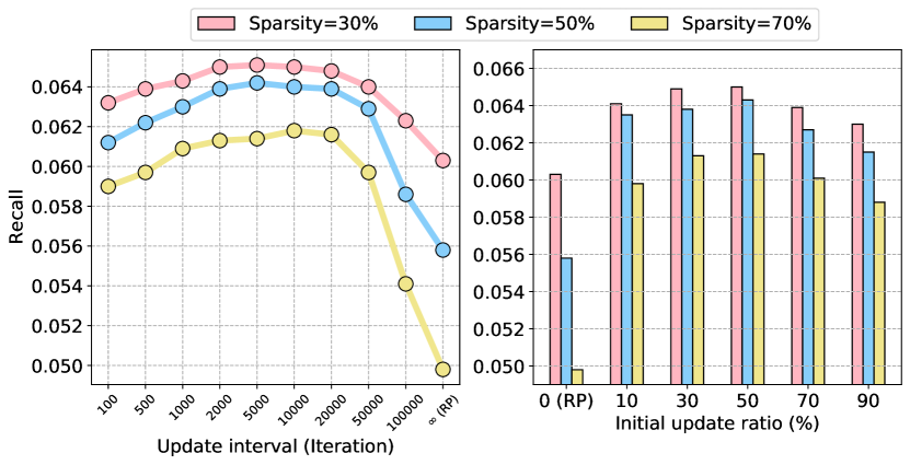
Figure 3. Performance over three sparsity levels. (Left): Performance over different update intervals $\Delta T$; (Right): Performance over different initial update ratios $\rho_{0}$.

Table 4. Comparisons with different decay functions.

Type	Amazon-book		Yelp2018		Gowalla
	Recall	NDCG	Recall	NDCG	Recall	NDCG
Cosine	0.0406	0.0316	0.0641	0.0527	0.1812	0.1546
Linear	0.0409	0.0317	0.0638	0.0525	0.1803	0.1538
No decay	0.0394	0.0307	0.0618	0.0507	0.1773	0.1518

4.4.2. Effect of Initial Update Ratio.

In DSL, $\rho_{0}$ refers to the initial ratio of pruning and growth in the exploration stage. In order to investigate its impact on DSL, we vary the value of $\rho_{0}$ across a range of small-to-large values Please note that $\rho_{0}=0$ means no update during training, so DSL also degenerates into RP. The results are depicted in Figure 3 (Right). We observe that as $\rho_{0}$ increases, the performance also shows a trend of increasing first and then decreasing. When $\rho_{0}$ is too small (e.g., $<$ 0.1), the scope of each exploration will be smaller, making it difficult to obtain a better model structure for each update. If we set $\rho_{0}$ too large (e.g., $>$ 0.7), it will also lead to poor performance. Too large adjustments will greatly influence the stability of training, such as destroying more critical weights or adding more trivial weights. In practice, we usually set $\rho_{0}$ in the range of $0.3\sim 0.5$. Within this range, DSL can achieve an appropriate degree of dynamic adjustment, enabling the model to remove/discover an appropriate amount of trivial/critical parameters during training.

4.4.3. Effect of Update Decay Function.

To substantiate the rationality of our choice of cosine annealing as the update decay function, we compare its performance with that of two alternative decay schedules: linear decay and no decay (i.e., where the update ratio remains constant throughout training). From the results in Table 4, we can find that updating with no decay makes it difficult to learn effective parameters. With each exploration, gradually reducing the update ratio is conducive to model convergence. Compared with the linear function, using the cosine annealing function as the decay function can make the update ratio drop more smoothly and bring more stable performance.

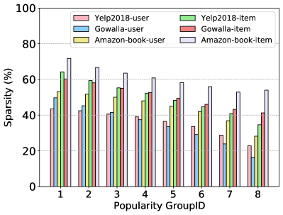
((a))

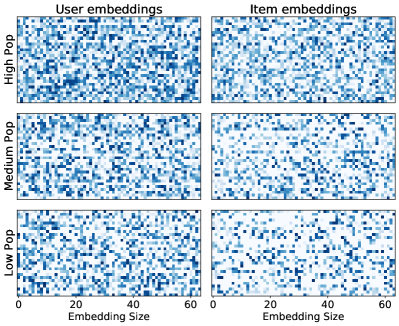
((b))

Figure 4. (Left): Sparsity distribution of the embeddings. Larger GroupIDs indicate more popular users or items. (Right): Embedding visualization with different popularity-levels. Darker color denotes larger weight magnitude and white color denotes the pruned weights.

4.5. Analysis and Visualization (RQ4)

4.5.1. Sparsity Distribution Analyses and Visualizations.

To study whether DSL can learn meaningful statistical regularities or patterns of sparsity, we conduct further analyses and visualizations about the sparse embeddings. Firstly, we sort and uniformly group users and items by popularity, and then count the average sparsity of the embeddings within each group, as shown in Figure 4 (Left). To illustrate the sparsity distribution more intuitively, we visualize the sparse embeddings with different popularity levels, as shown in Figure 4 (Right). We can observe that as the popularity increases, the sparsity of the embeddings learned by DSL gradually decreases. DSL can indeed discover interesting patterns: active users and popular items may carry more information, thereby requiring denser embeddings,and tend to heavily prune these over-parameterized embeddings to better preserve the performance.

4.5.2. Convergence Analyses

To better illustrate the influence of DSL on training convergence, we modify its parameters - initial update ratios $\rho_{0}$ and update intervals $\Delta T$ - and plot the corresponding loss decline curves for LightGCN and MultVAE models in Figure 5. At the beginning of training, DSL shows a rapid drop in training loss at a similar speed to the baseline and RP. However, as the number of iterations increases, the curves generated by DSL with varying update ratios and intervals exhibit slower convergence rates at higher update ratios or smaller update intervals. Compared to RP, DSL enables periodic parameter updates that facilitate faster convergence to lower loss values without impeding model convergence. Furthermore, compared to the baseline, while DSL does exhibit a slightly slower convergence speed compared to the baseline, it achieves comparable loss levels under nearly identical training epochs.

5. Related Work

Model Compression (Wang et al., 2019; Yan et al., 2021; Zhou et al., 2023; Molchanov et al., 2019; Evci et al., 2020; Qu et al., 2022) aims to obtain lightweight models by removing redundant weights. It becomes an effective solution to reduce model size in the fields of computer vision (Chen et al., 2020b; Sui et al., 2022a), graph learning (Sui et al., 2023a, 2022b, 2022c, b; Fang et al., 2023a, b; Chen et al., 2021a), and natural language processing (Chen et al., 2020a, 2022a, 2022b). Recently, the lottery ticket hypothesis (Frankle and Carbin, 2018; Wang et al., 2022) becomes an effective strategy to guide the model pruning. It states that dense randomly initialized networks contain sparse subnetworks (aka., winning tickets) that can be trained in isolation to achieve comparable performance. LTH-MRS (Wang et al., 2022) adopts an iterative pruning strategy to find the winning tickets in recommendation models, while still suffering from the expensiveness of multi-round retraining. PEP (Liu et al., 2021) proposes learnable pruning thresholds in model training, while the unstable learning process of thresholds makes it difficult to keep a controllable training budget and a stable performance. Distinct from them, we adjust the sparsity distribution of model weights while sticking to a fixed parameters budget, which can achieve both training and inference efficiency.

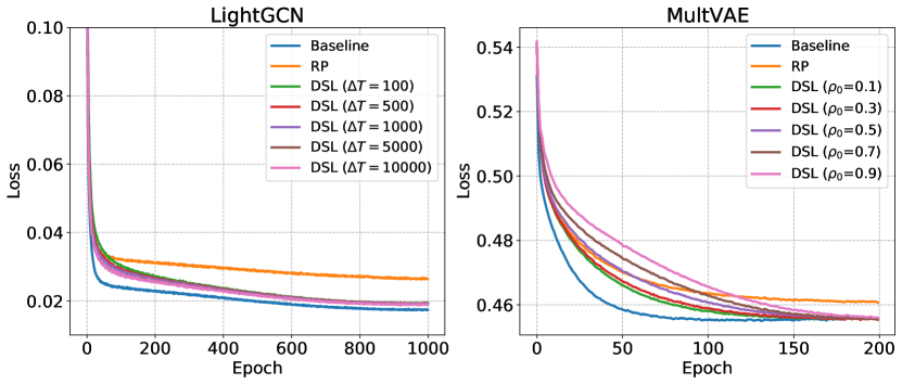
Figure 5. Convergence comparisons of training loss for the baseline model, RP, and DSL on different initial update ratios $\rho_{0}$ and update intervals $\Delta T$.

Efficient Recommendation is drawing widespread attention, due to the emergence of large-scale recommendation models (Wang et al., 2022; Chen et al., 2021b). Knowledge Distillation (KD) (Kweon et al., 2021; Kang et al., 2021, 2022; Tang and Wang, 2018) improves the performance of small-scale student models by distilling the knowledge from large-scale teacher models. BKD (Kweon et al., 2021) proposes a bidirectional distillation framework, which enhances the collaborations between teacher and student models. TKD (Kang et al., 2021) develops a topology distillation strategy, which transfers topological knowledge and guides students with diverse capacities. However, they need to pre-train large-scale teacher models, which still leads to expensive memory and training costs. Furthermore, there also exists a large gap in performance between student and teacher models (Tang and Wang, 2018). Automated Machine Learning (AutoML) (Chen et al., 2022d; Zheng et al., 2022c; Liu et al., 2021; Zhao et al., 2021b, a; Liu et al., 2020) improves inference efficiency by searching powerful and lightweight model architectures. AutoEmb (Zhao et al., 2021a) adopts a DARTS-based (Liu et al., 2018) optimization strategy to decide optimal embedding dimensions for users and items. ESAPN (Liu et al., 2020) leverages an automated reinforcement learning agent to search the embedding size of models. However, they require to predefine a search space with human prior knowledge. Meanwhile, the complex processes of optimization and performance estimation also result in an unaffordable computational cost. In contrast, our strategy can effectively trim down both training and inference overheads, by simply training a lightweight sparse model in an end-to-end way.

6. Conclusion and Future Work

In this work, we proposed DSL, which aims to trim down both the training and inference costs for recommendation models. Specifically, we introduced the concept of sparsity to the models, periodically and dynamically adjusted the sparsity distribution of model weights, and sticked to a fixed parameter budget throughout the entire learning lifecycle. Different from existing solutions, DSL achieved the intriguing prospect of “end-to-end” efficiency from training to inference. We conducted extensive experiments on diverse recommendation models with six benchmark datasets. The experimental results demonstrated that DSL can largely reduce the training cost, inference cost, and memory, with comparable recommendation performance. Finally, we also provided analyses and visualizations to demonstrate the effectiveness and rationality.

7. Acknowledgments

This research was supported in part by the National Natural Science Foundation of China (Grant No. 92370204) and Guangdong OPPO Mobile Telecommunications Co., Ltd .

References

- (1)
- Chen et al. (2022d) Bo Chen, Xiangyu Zhao, Yejing Wang, Wenqi Fan, Huifeng Guo, and Ruiming Tang. 2022d. Automated Machine Learning for Deep Recommender Systems: A Survey. arXiv preprint arXiv:2010.11929 (2022).
- Chen et al. (2023) Gang Chen, Jiawei Chen, Fuli Feng, Sheng Zhou, and Xiangnan He. 2023. Unbiased Knowledge Distillation for Recommendation. In WSDM. 976–984.
- Chen et al. (2022a) Liyi Chen, Zhi Li, Weidong He, Gong Cheng, Tong Xu, Nicholas Jing Yuan, and Enhong Chen. 2022a. Entity Summarization via Exploiting Description Complementarity and Salience. IEEE TNNLS (2022).
- Chen et al. (2020a) Liyi Chen, Zhi Li, Yijun Wang, Tong Xu, Zhefeng Wang, and Enhong Chen. 2020a. MMEA: entity alignment for multi-modal knowledge graph. In KSEM.
- Chen et al. (2022b) Liyi Chen, Zhi Li, Tong Xu, Han Wu, Zhefeng Wang, Nicholas Jing Yuan, and Enhong Chen. 2022b. Multi-modal Siamese Network for Entity Alignment. In SIGKDD.
- Chen et al. (2021a) Tianlong Chen, Yongduo Sui, Xuxi Chen, Aston Zhang, and Zhangyang Wang. 2021a. A unified lottery ticket hypothesis for graph neural networks. In ICML. PMLR, 1695–1706.
- Chen et al. (2022c) Tianlong Chen, Zhenyu Zhang, Santosh Balachandra, Haoyu Ma, Zehao Wang, Zhangyang Wang, et al. 2022c. Sparsity Winning Twice: Better Robust Generalization from More Efficient Training. In ICLR.
- Chen et al. (2020b) Xuxi Chen, Zhenyu Zhang, Yongduo Sui, and Tianlong Chen. 2020b. GANs Can Play Lottery Tickets Too. In ICLR.
- Chen et al. (2021b) Yankai Chen, Yifei Zhang, Yingxue Zhang, Huifeng Guo, Jingjie Li, Ruiming Tang, Xiuqiang He, and Irwin King. 2021b. Towards low-loss 1-bit quantization of user-item representations for top-k recommendation. arXiv preprint arXiv:2112.01944 (2021).
- Evci et al. (2020) Utku Evci, Trevor Gale, Jacob Menick, Pablo Samuel Castro, and Erich Elsen. 2020. Rigging the lottery: Making all tickets winners. In ICML. PMLR, 2943–2952.
- Evci et al. (2022) Utku Evci, Yani Ioannou, Cem Keskin, and Yann Dauphin. 2022. Gradient flow in sparse neural networks and how lottery tickets win. In AAAI, Vol. 36. 6577–6586.
- Fang et al. (2023a) Junfeng Fang, Wei Liu, Yuan Gao, Zemin Liu, An Zhang, Xiang Wang, and Xiangnan He. 2023a. Evaluating Post-hoc Explanations for Graph Neural Networks via Robustness Analysis. In NeurIPS. https://openreview.net/forum?id=eD534mPhAg
- Fang et al. (2023b) Junfeng Fang, Xiang Wang, An Zhang, Zemin Liu, Xiangnan He, and Tat-Seng Chua. 2023b. Cooperative Explanations of Graph Neural Networks. In WSDM. ACM, 616–624.
- Frankle and Carbin (2018) Jonathan Frankle and Michael Carbin. 2018. The Lottery Ticket Hypothesis: Finding Sparse, Trainable Neural Networks. In ICLR.
- Gou et al. (2021) Jianping Gou, Baosheng Yu, Stephen J Maybank, and Dacheng Tao. 2021. Knowledge distillation: A survey. International Journal of Computer Vision 129, 6 (2021), 1789–1819.
- Han et al. (2015) Song Han, Huizi Mao, and William J Dally. 2015. Deep compression: Compressing deep neural networks with pruning, trained quantization and huffman coding. arXiv preprint arXiv:1510.00149 (2015).
- He et al. (2020) Xiangnan He, Kuan Deng, Xiang Wang, Yan Li, Yongdong Zhang, and Meng Wang. 2020. Lightgcn: Simplifying and powering graph convolution network for recommendation. In SIGIR. 639–648.
- He et al. (2018) Xiangnan He, Xiaoyu Du, Xiang Wang, Feng Tian, Jinhui Tang, and Tat-Seng Chua. 2018. Outer product-based neural collaborative filtering. In IJCAI.
- He et al. (2017) Xiangnan He, Lizi Liao, Hanwang Zhang, Liqiang Nie, Xia Hu, and Tat-Seng Chua. 2017. Neural collaborative filtering. In WWW. 173–182.
- Kang et al. (2021) SeongKu Kang, Junyoung Hwang, Wonbin Kweon, and Hwanjo Yu. 2021. Topology distillation for recommender system. In SIGKDD. 829–839.
- Kang et al. (2022) SeongKu Kang, Dongha Lee, Wonbin Kweon, and Hwanjo Yu. 2022. Personalized Knowledge Distillation for Recommender System. Knowledge-Based Systems 239 (2022), 107958.
- Kweon et al. (2021) Wonbin Kweon, SeongKu Kang, and Hwanjo Yu. 2021. Bidirectional distillation for top-K recommender system. In WWW. 3861–3871.
- Lee and Kim (2021) Youngjune Lee and Kee-Eung Kim. 2021. Dual correction strategy for ranking distillation in top-n recommender system. In CIKM. 3186–3190.
- Liang et al. (2018) Dawen Liang, Rahul G Krishnan, Matthew D Hoffman, and Tony Jebara. 2018. Variational autoencoders for collaborative filtering. In WWW. 689–698.
- Liu et al. (2018) Hanxiao Liu, Karen Simonyan, and Yiming Yang. 2018. Darts: Differentiable architecture search. arXiv preprint arXiv:1806.09055 (2018).
- Liu et al. (2020) Haochen Liu, Xiangyu Zhao, Chong Wang, Xiaobing Liu, and Jiliang Tang. 2020. Automated embedding size search in deep recommender systems. In SIGIR. 2307–2316.
- Liu et al. (2021) Siyi Liu, Chen Gao, Yihong Chen, Depeng Jin, and Yong Li. 2021. Learnable embedding sizes for recommender systems. In ICLR.
- Loshchilov and Hutter (2016) Ilya Loshchilov and Frank Hutter. 2016. Sgdr: Stochastic gradient descent with warm restarts. arXiv preprint arXiv:1608.03983 (2016).
- Mao et al. (2021) Kelong Mao, Jieming Zhu, Xi Xiao, Biao Lu, Zhaowei Wang, and Xiuqiang He. 2021. UltraGCN: ultra simplification of graph convolutional networks for recommendation. In CIKM. 1253–1262.
- Molchanov et al. (2019) Pavlo Molchanov, Arun Mallya, Stephen Tyree, Iuri Frosio, and Jan Kautz. 2019. Importance estimation for neural network pruning. In CVPR. 11264–11272.
- Qin et al. (2008) A Kai Qin, Vicky Ling Huang, and Ponnuthurai N Suganthan. 2008. Differential evolution algorithm with strategy adaptation for global numerical optimization. IEEE transactions on Evolutionary Computation 13, 2 (2008), 398–417.
- Qu et al. (2022) Liang Qu, Yonghong Ye, Ningzhi Tang, Lixin Zhang, Yuhui Shi, and Hongzhi Yin. 2022. Single-shot Embedding Dimension Search in Recommender System. In SIGIR.
- Ruder (2016) Sebastian Ruder. 2016. An overview of gradient descent optimization algorithms. arXiv preprint arXiv:1609.04747 (2016).
- Savarese et al. (2020) Pedro Savarese, Hugo Silva, and Michael Maire. 2020. Winning the lottery with continuous sparsification. In NeurIPS, Vol. 33. 11380–11390.
- Sui et al. (2022a) Yongduo Sui, Tianlong Chen, Pengfei Xia, Shuyao Wang, and Bin Li. 2022a. Towards robust detection and segmentation using vertical and horizontal adversarial training. In IJCNN. IEEE, 1–8.
- Sui et al. (2023a) Yongduo Sui, Xiang Wang, Tianlong Chen, Meng Wang, Xiangnan He, and Tat-Seng Chua. 2023a. Inductive Lottery Ticket Learning for Graph Neural Networks. Journal of Computer Science and Technology (2023). https://doi.org/10.1007/s11390-023-2583-5
- Sui et al. (2022b) Yongduo Sui, Xiang Wang, Jiancan Wu, Min Lin, Xiangnan He, and Tat-Seng Chua. 2022b. Causal Attention for Interpretable and Generalizable Graph Classification. In SIGKDD.
- Sui et al. (2022c) Yongduo Sui, Xiang Wang, Jiancan Wu, An Zhang, and Xiangnan He. 2022c. Adversarial Causal Augmentation for Graph Covariate Shift. arXiv preprint arXiv:2211.02843 (2022).
- Sui et al. (2023b) Yongduo Sui, Qitian Wu, Jiancan Wu, Qing Cui, Longfei Li, Jun Zhou, Xiang Wang, and Xiangnan He. 2023b. Unleashing the Power of Graph Data Augmentation on Covariate Distribution Shift. In NeurIPS. https://openreview.net/pdf?id=hIGZujtOQv
- Tanaka et al. (2020) Hidenori Tanaka, Daniel Kunin, Daniel L Yamins, and Surya Ganguli. 2020. Pruning neural networks without any data by iteratively conserving synaptic flow. In NeurIPS, Vol. 33. 6377–6389.
- Tang and Wang (2018) Jiaxi Tang and Ke Wang. 2018. Ranking distillation: Learning compact ranking models with high performance for recommender system. In SIGKDD. 2289–2298.
- Tao et al. (2022) Ye Tao, Ying Li, Su Zhang, Zhirong Hou, and Zhonghai Wu. 2022. Revisiting Graph based Social Recommendation: A Distillation Enhanced Social Graph Network. In WWW. 2830–2838.
- Wang et al. (2019) Chaoqi Wang, Roger Grosse, Sanja Fidler, and Guodong Zhang. 2019. Eigendamage: Structured pruning in the kronecker-factored eigenbasis. In ICML. PMLR, 6566–6575.
- Wang et al. (2021) Chao Wang, Hengshu Zhu, Peng Wang, Chen Zhu, Xi Zhang, Enhong Chen, and Hui Xiong. 2021. Personalized and explainable employee training course recommendations: A bayesian variational approach. ACM Transactions on Information Systems (TOIS) 40, 4 (2021), 1–32.
- Wang et al. (2020) Chao Wang, Hengshu Zhu, Chen Zhu, Chuan Qin, and Hui Xiong. 2020. SetRank: A Setwise Bayesian Approach for Collaborative Ranking from Implicit Feedback.. In AAAI. 6127–6136.
- Wang et al. (2022) Yanfang Wang, Yongduo Sui, Xiang Wang, Zhenguang Liu, and Xiangnan He. 2022. Exploring lottery ticket hypothesis in media recommender systems. International Journal of Intelligent Systems 37, 5 (2022), 3006–3024.
- Wu et al. (2023) Likang Wu, Zhi Zheng, Zhaopeng Qiu, Hao Wang, Hongchao Gu, Tingjia Shen, Chuan Qin, Chen Zhu, Hengshu Zhu, Qi Liu, et al. 2023. A Survey on Large Language Models for Recommendation. arXiv preprint arXiv:2305.19860 (2023).
- Wu et al. (2016) Yao Wu, Christopher DuBois, Alice X Zheng, and Martin Ester. 2016. Collaborative denoising auto-encoders for top-n recommender systems. In WSDM. 153–162.
- Yan et al. (2021) Bencheng Yan, Pengjie Wang, Kai Zhang, Wei Lin, Kuang-Chih Lee, Jian Xu, and Bo Zheng. 2021. Learning Effective and Efficient Embedding via an Adaptively-Masked Twins-based Layer. In CIKM. 3568–3572.
- Yang et al. (2022) Chenxiao Yang, Junwei Pan, Xiaofeng Gao, Tingyu Jiang, Dapeng Liu, and Guihai Chen. 2022. Cross-Task Knowledge Distillation in Multi-Task Recommendation. In AAAI.
- You et al. (2019) Haoran You, Chaojian Li, Pengfei Xu, Yonggan Fu, Yue Wang, Xiaohan Chen, Richard G Baraniuk, Zhangyang Wang, and Yingyan Lin. 2019. Drawing early-bird tickets: Towards more efficient training of deep networks. arXiv preprint arXiv:1909.11957 (2019).
- Zhao et al. (2021a) Xiangyu Zhao, Haochen Liu, Wenqi Fan, Hui Liu, Jiliang Tang, Chong Wang, Ming Chen, Xudong Zheng, Xiaobing Liu, and Xiwang Yang. 2021a. Autoemb: Automated embedding dimensionality search in streaming recommendations. In ICDM. IEEE, 896–905.
- Zhao et al. (2021b) Xiangyu Zhao, Haochen Liu, Hui Liu, Jiliang Tang, Weiwei Guo, Jun Shi, Sida Wang, Huiji Gao, and Bo Long. 2021b. Autodim: Field-aware embedding dimension searchin recommender systems. In WWW. 3015–3022.
- Zheng et al. (2022c) Ruiqi Zheng, Liang Qu, Bin Cui, Yuhui Shi, and Hongzhi Yin. 2022c. AutoML for Deep Recommender Systems: A Survey. arXiv preprint arXiv:2203.13922 (2022).
- Zheng et al. (2023a) Zhi Zheng, Zhaopeng Qiu, Xiao Hu, Likang Wu, Hengshu Zhu, and Hui Xiong. 2023a. Generative job recommendations with large language model. arXiv preprint arXiv:2307.02157 (2023).
- Zheng et al. (2022a) Zhi Zheng, Zhaopeng Qiu, Hui Xiong, Xian Wu, Tong Xu, Enhong Chen, and Xiangyu Zhao. 2022a. DDR: Dialogue Based Doctor Recommendation for Online Medical Service. In SIGKDD. 4592–4600.
- Zheng et al. (2022b) Zhi Zheng, Zhaopeng Qiu, Tong Xu, Xian Wu, Xiangyu Zhao, Enhong Chen, and Hui Xiong. 2022b. CBR: context bias aware recommendation for debiasing user modeling and click prediction. In WWW. 2268–2276.
- Zheng et al. (2023b) Zhi Zheng, Ying Sun, Xin Song, Hengshu Zhu, and Hui Xiong. 2023b. Generative Learning Plan Recommendation for Employees: A Performance-aware Reinforcement Learning Approach. In RecSys. 443–454.
- Zheng et al. (2021) Zhi Zheng, Chao Wang, Tong Xu, Dazhong Shen, Penggang Qin, Baoxing Huai, Tongzhu Liu, and Enhong Chen. 2021. Drug package recommendation via interaction-aware graph induction. In WWW. 1284–1295.
- Zheng et al. (2023c) Zhi Zheng, Chao Wang, Tong Xu, Dazhong Shen, Penggang Qin, Xiangyu Zhao, Baoxing Huai, Xian Wu, and Enhong Chen. 2023c. Interaction-aware drug package recommendation via policy gradient. ACM Transactions on Information Systems (TOIS) 41, 1 (2023), 1–32.
- Zhou et al. (2023) You Zhou, Xiujing Lin, Xiang Zhang, Maolin Wang, Gangwei Jiang, Huakang Lu, Yupeng Wu, Kai Zhang, Zhe Yang, Kehang Wang, et al. 2023. On the Opportunities of Green Computing: A Survey. arXiv preprint arXiv:2311.00447 (2023).
- Zhu and Gupta (2018) Michael Zhu and Suyog Gupta. 2018. To prune, or not to prune: exploring the efficacy of pruning for model compression. In ICLR.