Do we need decay-preserving error estimate for solving parabolic equations with initial singularity?

Abstract

Solutions exhibiting weak initial singularities arise in various equations, including diffusion and subdiffusion equations. When employing the well-known L1 scheme to solve subdiffusion equations with weak singularities, numerical simulations reveal that this scheme exhibits varying convergence rates for different choices of model parameters (i.e., domain size, final time $T$, and reaction coefficient $\kappa$). This elusive phenomenon is not unique to the L1 scheme but is also observed in other numerical methods for reaction-diffusion equations such as the backward Euler (IE) scheme, Crank-Nicolson (C-N) scheme, and two-step backward differentiation formula (BDF2) scheme. The existing literature lacks an explanation for the existence of two different convergence regimes, which has puzzled us for a long while and motivated us to study this inconsistency between the standard convergence theory and numerical experiences. In this paper, we provide a general methodology to systematically obtain error estimates that incorporate the exponential decaying feature of the solution. We term this novel error estimate the ‘decay-preserving error estimate’ and apply it to the aforementioned IE, C-N, and BDF2 schemes. Our decay-preserving error estimate consists of a low-order term with an exponential coefficient and a high-order term with an algebraic coefficient, both of which depend on the model parameters. Our estimates reveal that the varying convergence rates are caused by a trade-off between these two components in different model parameter regimes. By considering the model parameters, we capture different states of the convergence rate that traditional error estimates fail to explain. This approach retains more properties of the continuous solution. We validate our analysis with numerical results.

Keywords: diffusion equation, subdiffusion equation, weak initial singularity, decay-preserving error estimate, convergence rate, model parameters

1 Introduction

Many studies have been carried out on numerical analysis of the following linear reaction subdiffusion equations

$$\partial_{t}^{\alpha}u-\Delta u =\kappa u+f, x\in\Omega,\;t\in(0,T],$$ (1.1)

$$u(x,t) =0, x\in\partial\Omega,\;t\in(0,T],$$

$$u(x,0) =u_{0}(x), x\in\bar{\Omega},$$

where the reaction coefficient $\kappa$ is a given constant, and $\partial_{t}^{\alpha}$ denotes the fractional Caputo’s derivative of order $\alpha$ with respect to $t$, namely

$$\partial_{t}^{\alpha}u({x},t)=\frac{1}{\Gamma(1-\alpha)}\int_{0}^{t}\frac{\partial_{s}u({x},s)}{(t-s)^{\alpha}}ds,\quad 0<\alpha<1.$$

Diffusion is one of the most prominent transport mechanisms in nature. The classical diffusion models generally describe the Brownian motion of particles. However, over the last few decades, numerous experimental findings suggest that the Brownian motion assumption may not be adequate for accurately describing some physical processes, such as anomalous diffusion or non-Gaussian process. Instead, these processes are better described by the model (1.1). For a comprehensive exploration of various applications and physical modeling, one can refer to the surveys in [15, 16] and the monograph [6].

In any numerical methods for solving problem (1.1), a key consideration is that the solution exhibits a weak singularity near the initial time $t=0$ even though the initial value is smooth. Specifically, if $u_{0}(x)\in H^{1}_{0}(\Omega)\cap H^{2}(\Omega)$, the solution of problem (1.1) with $f=0$ satisfies [5]

$$\|\partial_{t}u(t)\|_{L^{2}(\Omega)}\leq Ct^{\alpha-1}.$$ (1.2)

Under the regularity condition (1.2), the convergence rate with the maximum norm in time is proven to be $\mathcal{O}(\tau^{\alpha})$ for various numerical schemes, such as the L1 and L2-type [9, 17, 10, 7] and convolution quadrature schemes [5, 13]. Furthermore, the point-wise error estimate of the L1 scheme at time $t=t_{n}$ is established as $\mathcal{O}(\tau t_{n}^{\alpha-1})$ in [2, 8], implying that the L1 scheme with a smooth initial value is first-order convergent at the final time level. Further discussions can be found in [20, 3, 4, 14]. An example is widely used to numerically verify the theory by taking $\Omega=(0,L)$, and the exact solution of problem (1.1) is constructed as

$$u=t^{\alpha}\sin(\pi x/L).$$ (1.3)

In the simulation, we use the L1 scheme to discretize the Caputo derivative with N uniformly distributed grid points, and use the finite difference method in space with $M$ grid points. Table 1 displays temporal convergence rates of the L1 scheme for a fixed time level $t_{N}=T$, $\alpha=0.5$ and $M=20000$. An interesting and puzzling phenomenon is observed in Table 1 that the convergence rates are influenced by the choices of model parameters, i.e., the interval length $L$, the final time $T$ and the reaction coefficient $\kappa$. Specifically, the convergence order is $\mathcal{O}(\tau)$ while choosing $L=\pi,\kappa=0,-1$, which is consistent with the existing results of $\mathcal{O}(\tau t_{n}^{\alpha-1})$ in [2, 8]. On the other hand, the convergence rate approaches $\mathcal{O}(\tau^{2-\alpha})$ for $T=10,L=1,\kappa=-8,N=64$, consistent with the results in [12, 18].

Table 1: The empirical convergence rates of L1 scheme by taking various parameters $L$, $\kappa$ and $T$.

  $N$ $L=1$ $L=\pi$ $\kappa=1$ $\kappa=0$ $\kappa=-8$ $\kappa=1$ $\kappa=0$ $\kappa=-8$ 64 1.28 1.29 1.36 1.00 1.06 1.28 $T=1$ 128 1.24 1.25 1.32 1.00 1.05 1.24 256 1.19 1.20 1.28 1.00 1.03 1.19 512 1.15 1.16 1.23 1.00 1.02 1.15 64 1.40 1.41 1.45 1.00 1.16 1.40 $T=10$ 128 1.37 1.38 1.43 1.00 1.12 1.37 256 1.33 1.34 1.40 1.00 1.09 1.33 512 1.30 1.31 1.37 1.00 1.07 1.29  

The results in Table 1 indicate that the different model parameters (i.e., domain sizes, final time $T$, and reaction coefficient $\kappa$) may lead to varying convergent rates with respect to $N$. This elusive phenomena cannot be explained by error estimates in previous literatures, as their theories do not consider the influence of model parameters. This inconsistence between numerical experiments and theoretical analysis has puzzled us for a long time, motivating further investigation to unveil the underlying dynamics and solve the mystery. It is natural to inquire whether a similar behavior occurs in the classical diffusion equation (i.e., $\alpha=1$ in (1.1)):

$$\partial_{t}u-\Delta u =\kappa u+f, x\in\Omega,\;t\in(0,T],$$ (1.4)

$$u(x,t) =0, x\in\partial\Omega,\;t\in[0,T],$$

$$u(x,0) =u_{0}(x), x\in\bar{\Omega}.$$

In the simulation, we use the same exact solution (1.3) with $\alpha=0.5$ for (1.4), which also satisfies the singularity condition (1.2). Taking the implicit Euler scheme as an example, Table 2 shows that the convergence rate is $\mathcal{O}(\tau^{\alpha})$ for $L=\pi,T=1$, and various $\kappa$ values, while it is $\mathcal{O}(\tau)$ for $L=1$ and different $T$ and $\kappa$. On the other hand for $L=\pi$ and $T=10$, the convergence rate is $\mathcal{O}(\tau)$ for $\kappa=0,-8$, and is changing to $\mathcal{O}(\tau^{\alpha})$ for $\kappa=1$. Similar phenomena are observed in simulations using C-N and BDF2 schemes, where the convergence rates change with different model parameters. The results in Tables 1 and 2 suggest that it is a common phenomenon for both diffusion and subdiffusion equations when an initial singularity is present.

Table 2: The empirical convergence rates of implicit Euler scheme by taking various $L$, $\kappa$ and $T$.

  $N$ $L=1$ $L=\pi$ $\kappa=1$ $\kappa=0$ $\kappa=-1$ $\kappa=1$ $\kappa=0$ $\kappa=-1$ 64 1.03 1.03 1.02 0.47 0.50 0.56 $T=1$ 128 1.00 1.01 1.01 0.48 0.50 0.54 256 0.98 0.99 1.00 0.49 0.50 0.53 512 0.96 0.98 1.00 0.49 0.50 0.52 64 1.01 1.01 1.01 0.47 1.03 1.01 $T=10$ 128 1.01 1.01 1.01 0.48 1.01 1.01 256 1.00 1.00 1.00 0.49 1.00 1.00 512 1.00 1.00 1.00 0.49 0.99 1.00  

The existing theory fails to explain the observed variations in convergence rates with different model parameters. This discrepancy motivates us to develop a methodology for systematically describing various convergence regimes, spanning from lower to high orders. To the end, we first eliminate the effect of the spatial domain by considering the corresponding ordinary differential equations (ODEs) with an initial singularity. We establish refined decay-preserving error estimates for the widely used implicit Euler scheme, C-N scheme, and BDF2 scheme. Specifically for $\kappa<0$, the novel decay-preserving error estimates are proven to be

$$|e^{n}|\leq e^{C\kappa t_{n}}|e^{0}|+C_{u,\alpha}\Big{(}e^{C\kappa t_{n}}\tau^{\alpha}+Ct_{n-1}^{\alpha-1}\tau^{k}\Big{)},$$ (1.5)

where $k=1$ represents for implicit Euler scheme and $k=2$ for C-N and BDF2 schemes. Afterwards, leveraging the corresponding eigenvalue problem, we extend the refined decay-preserving error estimates to diffusion problems with an initial singularity. Subsequently, we conduct numerical experiments to further demonstrate and validate our decay-preserving error estimates, which can effectively capture the characteristics of various convergence regimes for different $L,\kappa$, and $T$. Consequently, we establish an analyzable connection between the model parameters and the primary features of convergence rates. Furthermore, we put forward a conjecture regarding the preserving error estimate for subdiffusion equations.

The organization of this paper is as follows. In Section 2, we present a general methodology for systematically obtaining new decay-preserving error estimates for widely used IE, C-N, and BDF2 schemes applied to ODEs (2.1). In Section 3, by incorporating the eigenvalue problem (3.1), we extend these decay-preserving error estimates to reaction-diffusion equations (1.4). Section 4 proposes a conjecture for the decay-preserving error estimate for reaction-subdiffusion equation (1.1). Based on these decay-preserving error estimates, we further discuss the connections between convergence regimes and model parameters. Furthermore, we provide numerical examples to illustrate and validate our theoretical results. Section 5 contains detailed proofs of the main results, and the paper concludes with a summary in Section 6.

2 Decay-preserving error estimate for ODE solvers

We first present the error estimates for widely used schemes, namely, the implicit Euler scheme, Crank-Nicolson (C-N) scheme and BDF2 scheme, applied to solve the following ODEs

$$u_{t}=\kappa u+f,\quad t>0$$ (2.1)

with the initial value $u(0)=u_{0}$ and a given constant $\kappa\in\mathbb{R}$. Assume that the solution of (2.1) satisfies the following regularity

$$|\partial^{k}u|\leq C_{u,\alpha}t^{-k+\alpha},\ k=1,2,3\text{ and }\;0<\alpha<1.$$ (2.2)

As the first step, we generate a grid by

$$t_{n}=n\tau,\quad n=0,1,\dots,N,\quad\tau=T/N.$$ (2.3)

At a grid point, we take $U^{n}$ as the approximate value of the true solution of $u^{n}=u(t_{n})$. For any time sequence $\{v^{n}\}_{n=0}^{N}$, we introduce the following notations

$$\nabla_{\tau}v^{n}=v^{n}-v^{n-1},\quad v^{n-\frac{1}{2}}=\frac{1}{2}(v^{n}+v^{n-1}),\quad D_{2}v^{n}:=\frac{3v^{n}-4v^{n-1}+v^{n-2}}{2\tau}.$$ (2.4)

The discretizations are given by

$$\frac{1}{\tau}\nabla_{\tau}U^{n}=\kappa U^{n}+f^{n},$$ Implicit Euler scheme (2.5)

$$\frac{1}{\tau}\nabla_{\tau}U^{n}=\kappa U^{n-\frac{1}{2}}+f^{n-\frac{1}{2}},$$ C-N scheme (2.6)

$$D_{2}U^{n}=\kappa U^{n}+f^{n},\;\;n\geq 2,$$ BDF2 scheme (2.7)

with initial value $U^{0}=u_{0}$. Noting BDF2 needs two initial values, we here use IE scheme to compute $U^{1}$.

Before the numerical analysis of schemes (2.5),(2.6) and (2.7), we first present a lemma which will be used frequently in later proofs.

Lemma 2.1.

Given constants $\varrho>1$ and $\beta<-1$, let

$$I_{n} =\sum_{k=2}^{n-1}\tau\varrho^{-(n-k-1)}t_{k}^{\beta},$$ (2.8)

where $t_{k}$ is defined in (2.3). Then it holds for $n\geq 4$ that

$$I_{n} \leq\frac{-1}{\beta+1}\Big{(}(2^{-(\beta+1)}(1-\varrho^{-(\frac{n}{2}-1)})-1)t_{n-1}^{\beta+1}+\varrho^{-(\frac{n}{2}-2)}\tau^{\beta+1}\Big{)}.$$ (2.9)

Proof. Applying the inequality ${t_{k-1}^{\beta+1}-t_{k}^{\beta+1}}\geq-(\beta+1){\tau}t_{k}^{\beta}$ to (2.8), one has

$$I_{n} \leq\frac{-1}{\beta+1}\Big{(}\sum_{k=2}^{n-1}\varrho^{-(n-k-1)}(t_{k-1}^{\beta+1}-t_{k}^{\beta+1})\Big{)}$$

$$=\frac{-1}{\beta+1}\Big{(}(\varrho-1)\sum_{k=2}^{n-2}\varrho^{-(n-k-1)}t_{k}^{\beta+1}+\varrho^{-(n-3)}\tau^{\beta+1}-t_{n-1}^{\beta+1}\Big{)}.$$ (2.10)

Set the integer $n_{0}=[\frac{n}{2}]$. It is easy to check $t_{n_{0}}\leq\frac{t_{n}}{2}\leq t_{n_{0}+1}$ and

$$(\varrho-1)\sum_{k=2}^{n-2}\varrho^{-(n-k-1)}t_{k}^{\beta+1} =(\varrho-1)\big{(}\sum_{k=2}^{n_{0}}\varrho^{-(n-k-1)}t_{k}^{\beta+1}+\sum_{k=n_{0}+1}^{n-2}\varrho^{-(n-k-1)}t_{k}^{\beta+1}\big{)}$$ (2.11)

$$\leq\tau^{\beta+1}(\varrho^{-(n-n_{0}-2)}-\varrho^{-(n-3)})+t_{n_{0}+1}^{\beta+1}(1-\varrho^{-(n-n_{0}-2)})$$

$$\leq\tau^{\beta+1}(\varrho^{-(\frac{n}{2}-2)}-\varrho^{-(n-3)})+(\frac{t_{n}}{2})^{\beta+1}(1-\varrho^{-(\frac{n}{2}-1)}).$$ (2.12)

The proof is completed by inserting (2.12) into (2.10).  

Remark 1.

In summation (2.8), the weight of $t_{2}$ is $\varrho^{-(n-3)}$, and the weight of $t_{n-1}$ is 1. This implies that the weights are in different scales for different $t_{k}$ when $n\gg 1$. The aim of introducing an integer $n_{0}$ is to divide the summation into two parts in (2.11), allowing one to estimate the two scales in (2.9), respectively. In other words, the weight of the leading order exponentially decays, while the second order (constant quantity) algebraically decays with respect to $n$. The two-scale estimate in Lemma 2.1 will play a key role in proving our decay-preserving error estimates.

2.1 Decay-preserving error estimate for implicit Euler scheme

We consider the case of $\kappa<0$. It follows from (2.5) that

$$(1-\kappa\tau)U^{n}=U^{n-1}+\tau f^{n},$$

which yields

$$U^{n}=(1-\kappa\tau)^{-n}U^{0}+\tau\sum_{k=1}^{n}(1-\kappa\tau)^{-(n+1-k)}f^{k}.$$

Set the error $e^{n}=u^{n}-U^{n}$. The error satisfies the following equation

$$e^{n}=(1-\kappa\tau)^{-n}e^{0}+\tau\sum_{k=1}^{n}(1-\kappa\tau)^{-(n+1-k)}R^{k},$$ (2.13)

with the truncation error $R^{k}=-\frac{1}{\tau_{k}}\int_{t_{k-1}}^{t_{k}}(s-t_{k-1})u^{\prime\prime}(s){\;\rm{d}}s.$ Following regularity condition (2.2), one has

$$|R^{1}|\leq\tau^{\alpha-1}\;\text{ and }\;|R^{k}|\leq C_{u,\alpha}\tau t_{k-1}^{\alpha-2},\quad k\geq 2.$$ (2.14)

Lemma 2.2.

For any $0<\tau\leq-1/\kappa$ and $\upsilon\geq 0$, it holds that

$$e^{\kappa\upsilon\tau}\leq(1-\kappa\tau)^{-\upsilon}\leq e^{\frac{\kappa\upsilon\tau}{2}}.$$ (2.15)

Proof. For any $x\geq 0$, the direct calculation shows that

$$x-\frac{x^{2}}{2}\leq\ln(1+x)\leq x\quad\text{and}\quad(1+x)^{1/x}=e^{\frac{\ln(1+x)}{x}},$$

which implies $e^{1-x/2}\leq(1+x)^{1/x}\leq e.$ If $0\leq x\leq 1$, we further have $e^{1/2}\leq(1+x)^{1/x}\leq e$.

Thus, setting $x=-\kappa\tau\leq 1$ and noting $(1-\kappa\tau)^{-\upsilon}=\big{(}(1-\kappa\tau)^{-\frac{1}{\kappa\tau}}\big{)}^{\kappa\upsilon\tau}$, we immediately have the inequalities in (2.15). The proof is completed.  

Theorem 2.1.

Let $u^{n}$ and $U^{n}$ be solutions to (2.1) and (2.5) respectively. Then for $-\kappa\tau<1$ it holds

$$|e^{n}|\leq e^{\kappa t_{n}/2}|e^{0}|+C_{u,\alpha}\Big{(}C_{1}e^{\kappa t_{n}/4}\tau^{\alpha}+C_{2}t_{n-1}^{\alpha-1}\tau\Big{)},$$ (2.16)

where $C_{1}:=\frac{2}{1-\alpha}+3e^{\frac{\kappa t_{n}}{4}}$ and

$$C_{2}:=\Big{\{}\begin{array}[]{cc}\frac{1}{1-\alpha}(2^{1-\alpha}(1-e^{\frac{\kappa t_{n}}{4}})-1),&t_{n}>\frac{4}{\kappa}\ln(1-2^{\alpha-1}),\\ 0,&t_{n}\leq\frac{4}{\kappa}\ln(1-2^{\alpha-1}).\end{array}$$

Proof. Inserting (2.14) into (2.13), one has

$$|e^{n}|\leq(1-\kappa\tau)^{-n}|e^{0}|+C_{u,\alpha}\Big{(}S_{n}\tau+(1-\kappa\tau)^{-n}(2-\kappa\tau)\tau^{\alpha}\Big{)},$$ (2.17)

where $S_{n}$ is defined by

$$S_{n}\;=\;(1-\kappa\tau)^{-(n+1)}\sum_{k=3}^{n}\tau(1-\kappa\tau)^{k}t_{k-1}^{\alpha-2}\;=\;(1-\kappa\tau)^{-1}\sum_{k=2}^{n-1}\tau(1-\kappa\tau)^{-(n-k-1)}t_{k}^{\alpha-2}.$$

Taking $\varrho=1-\kappa\tau,\beta=\alpha-2$, it follows from Lemma 2.1 that

$$S_{n} \leq\frac{1}{(1-\alpha)(1-\kappa\tau)}\Big{(}(2^{1-\alpha}(1-(1-\kappa\tau)^{-(\frac{n}{2}-1)})-1)t_{n}^{\alpha-1}+(1-\kappa\tau)^{-(\frac{n}{2}-2)}\tau^{\alpha-1}\Big{)}.$$

Substituting the above bound of $S_{n}$ into (2.17), one has

$$|e^{n}|\leq(1-\kappa\tau)^{-n}|e^{0}|+C_{u,\alpha}\Big{(}C_{1}(\tau,n)(1-\kappa\tau)^{-\frac{n}{2}}\tau^{\alpha}+C_{2}(\tau,n)t_{n-1}^{\alpha-1}\tau\Big{)},$$

where $C_{1}(\tau,n):=\frac{1-\kappa\tau}{1-\alpha}+(2-\kappa\tau)(1-\kappa\tau)^{-\frac{n}{2}},\;C_{2}(\tau,n):=\frac{1}{1-\alpha}(2^{1-\alpha}(1-(1-\kappa\tau)^{-\frac{n}{2}})-1).$

Noting $\tau\leq-1/\kappa$ and using Lemma 2.2, we have

$$C_{1}(\tau,n)\leq\frac{2}{1-\alpha}+3e^{\frac{\kappa t_{n}}{4}}:=C_{1},\qquad C_{2}(\tau,n)\leq\frac{1}{1-\alpha}(2^{1-\alpha}(1-e^{\frac{\kappa t_{n}}{4}})-1)\leq C_{2}.$$

Thus, the proof is completed.  

2.2 Decay-preserving error estimate for C-N scheme

We now consider the decaying error estimate for C-N scheme with $\kappa<0$. It follows from (2.6) that

$$(1-\kappa\tau/2)U^{n}=(1+\kappa\tau/2)U^{n-1}+\tau f^{n-\frac{1}{2}},$$

which yields

$$U^{n}=\psi_{\tau}^{-n}U^{0}+\tau(1-\frac{\kappa\tau}{2})^{-1}\sum_{k=1}^{n}\psi_{\tau}^{-(n-k)}f^{k-\frac{1}{2}},$$ (2.18)

where $\psi_{\tau}:=(1-\frac{\kappa\tau}{2})/(1+\frac{\kappa\tau}{2})$. Let $e^{n}=u^{n}-U^{n}$. The error satisfies

$$e^{n}=\psi_{\tau}^{-n}e^{0}+\tau(1-\frac{\kappa\tau}{2})^{-1}\sum_{k=1}^{n}\psi_{\tau}^{-(n-k)}(R_{1}^{k}+R_{2}^{k}),$$ (2.19)

where the truncation errors are respectively given by $R_{1}^{k}:=\nabla_{\tau}U^{k}/\tau-u^{\prime}(t_{k-\frac{1}{2}})\;\text{and}\;R_{2}^{k}:=U^{k-\frac{1}{2}}-u(t_{k-\frac{1}{2}}).$ The direct calculation shows that the truncations errors can be exactly expressed by

$$R_{1}^{k} =\frac{1}{2\tau}\big{(}\int_{t_{k-\frac{1}{2}}}^{t_{k}}(t_{k}-s)^{2}u^{\prime\prime\prime}(s){\;\rm{d}}s+\int^{t_{k-\frac{1}{2}}}_{t_{k-1}}(s-t_{k-1})^{2}u^{\prime\prime\prime}(s){\;\rm{d}}s\big{)},$$

$$R_{2}^{k} =\frac{1}{2}\big{(}\int_{t_{k-\frac{1}{2}}}^{t_{k}}(t_{k}-s)u^{\prime\prime}(s){\;\rm{d}}s+\int^{t_{k-\frac{1}{2}}}_{t_{k-1}}(s-t_{k-1})u^{\prime\prime}(s){\;\rm{d}}s\big{)}.$$

Using the regularity condition (2.2), one has the following error bounds

$$R_{1}^{k}+R_{2}^{k}\leq\Big{\{}\begin{array}[]{cc}C_{u,\alpha}\tau^{\alpha-1},&k=1,\\ C_{u,\alpha}\tau^{2}t_{k-1}^{\alpha-3},&k\geq 2.\end{array}$$ (2.20)

Lemma 2.3.

For any $0<-\kappa\tau\leq 1$ and $\upsilon\geq 0$, it holds that

$$e^{\frac{7}{6}\kappa\upsilon\tau}\leq\psi_{\tau}^{-\upsilon}\leq e^{\kappa\upsilon\tau},$$ (2.21)

where $\psi_{\tau}=(1-\frac{\kappa\tau}{2})/(1+\frac{\kappa\tau}{2})$.

Proof. Noting that $(1+x)^{\frac{1}{x}}=e^{\frac{\ln(1+x)}{x}}=e^{1-\frac{1}{x}\int_{0}^{x}\frac{(x-s)}{(1+s)^{2}}{\;\rm{d}}s}\;\text{and}\;(1-x)^{\frac{1}{x}}=e^{-1-\frac{1}{x}\int_{0}^{x}\frac{(x-s)}{(1-s)^{2}}{\;\rm{d}}s},\forall 0<x<1,$ we then have $\big{(}\frac{1-x}{1+x}\big{)}^{\frac{1}{x}}=e^{-2-\frac{1}{x}\int_{0}^{x}\frac{4s(x-s)}{(1-s^{2})^{2}}{\;\rm{d}}s}.$ For any $0<x\leq\frac{1}{2}$, note that

$$\frac{1}{x}\int_{0}^{x}\frac{4s(x-s)}{(1-s^{2})^{2}}{\;\rm{d}}s \leq\frac{4}{(1-x^{2})^{2}x}\int_{0}^{x}s(x-s){\;\rm{d}}s=\frac{2}{3(\frac{1}{x}-x)^{2}}<\frac{1}{3},$$

we further have

$$e^{-\frac{7}{3}}\leq\Big{(}\frac{1-x}{1+x}\Big{)}^{\frac{1}{x}}\leq e^{-2}.$$ (2.22)

By the definition of

$$\psi_{\tau}^{-\upsilon}=\Big{(}\big{(}\frac{1+\frac{\kappa\tau}{2}}{1-\frac{\kappa\tau}{2}}\big{)}^{-\frac{2}{\kappa\tau}}\Big{)}^{-\frac{\kappa\upsilon\tau}{2}},$$ (2.23)

we have $e^{\frac{7}{6}\kappa\upsilon\tau}\leq\psi_{\tau}^{-\upsilon}\leq e^{\kappa\upsilon\tau}$ in analogy of (2.22). The proof is completed.  

Theorem 2.2.

Let $u^{n}$ and $U^{n}$ be solutions to (2.1) and (2.6) respectively. Then for $0<-\kappa\tau<1$ it holds

$$|e^{n}|\leq e^{\kappa t_{n}}|e^{0}|+C_{u,\alpha}\Big{(}C_{3}e^{\frac{\kappa t_{n}}{2}}\tau^{\alpha}+C_{4}t_{n}^{\alpha-2}\tau^{2}\Big{)},$$ (2.24)

where $C_{3}:=\frac{9}{2-\alpha}+12e^{\frac{\kappa t_{n}}{2}}$ and

$$C_{4}:=\Big{\{}\begin{array}[]{cc}\frac{1}{2-\alpha}(2^{2-\alpha}(1-e^{\frac{7\kappa t_{n}}{12}})-1),&t_{n}>\frac{12}{7\kappa}\ln(1-2^{\alpha-2}),\\ 0,&t_{n}\leq\frac{12}{7\kappa}\ln(1-2^{\alpha-2}).\end{array}$$

Proof. Inserting the truncation error bounds (2.20) into (2.19), one has

$$|e^{n}|\;\leq\;\psi_{\tau}^{n}|e^{0}|+C_{u,\alpha}\Big{(}S_{n}\tau^{2}+(\psi_{\tau}+1)\psi_{\tau}^{-(n-1)}\tau^{\alpha}\Big{)},$$ (2.25)

where

$$S_{n}\;=\;\sum_{k=3}^{n}\tau\psi_{\tau}^{-(n-k)}t_{k-1}^{\alpha-3}\;=\;\sum_{k=2}^{n-1}\tau\psi_{\tau}^{-(n-k-1)}t_{k}^{\alpha-3}.$$ (2.26)

The case of $n\leq 3$ can be easily estimated and here we only assume $n\geq 4$.

For $0<-\kappa\tau<1$, taking $\varrho=\psi_{\tau}$ and $\beta=\alpha-3$ in Lemma 2.1, and applying Lemma 2.3 to (2.26), we have

$$S_{n}\;\leq\;\frac{1}{2-\alpha}\Big{(}(2^{2-\alpha}(1-e^{\frac{7\kappa t_{n}}{12}})-1)t_{n}^{\alpha-2}+9e^{\frac{\kappa t_{n}}{2}}\tau^{\alpha-2}\Big{)},$$ (2.27)

where $\psi_{\tau}\leq 3$ is used. Again, from Lemma (2.3) and the assumption $-\kappa\tau<1$, we have

$$(\psi_{\tau}+1)\psi_{\tau}^{-(n-1)}\leq 12e^{\kappa t_{n}}.$$ (2.28)

The proof is completed by inserting (2.27) and (2.28) into (2.25).  

2.3 Decay-preserving error estimate for BDF2 scheme

We now consider the decaying error estimate for BDF2 scheme with $\kappa<0$. From (2.7), one has

$$U^{1}-U^{0} =\kappa\tau U^{1}+\tau f^{1},$$ (2.29)

$$\frac{3}{2}U^{n}-2U^{n-1}+\frac{1}{2}U^{n-2} =\kappa\tau U^{n}+\tau f^{n},\quad n\geq 2.$$ (2.30)

Set $F^{k}=f^{k}(k\geq 3)$ and $F^{2}=f^{2}-\frac{U^{0}}{2\tau},\;F^{1}=f^{1}+\frac{U^{0}}{\tau}$. We further introduce the following notations, say the BDF2 kernels, as $A^{(1)}_{0}=1-\kappa\tau$ and for $n\geq 2$

$$A^{(n)}_{0}=\frac{3}{2}-\kappa\tau,\quad A^{(n)}_{1}=-2,\quad A^{(n)}_{2}=\frac{1}{2},\quad A^{(n)}_{j}=0\;(3\leq j<n).$$ (2.31)

Thus, BDF2 scheme (2.29)-(2.30) can be reformulated into the following convolution form

$$\sum_{j=1}^{k}A^{(n)}_{n-k}U^{j}=\tau F^{k}.$$

Set the error $e^{n}=u^{n}-U^{n}$. The error satisfies the governing equation as

$$\sum_{j=1}^{k}A^{(k)}_{k-j}e^{j}=\tau R^{k},$$ (2.32)

where

$$R^{1}=\eta^{1}+e^{0}/\tau,\;R^{2}=\eta^{2}-e^{0}/(2\tau)\quad\text{and}\quad R^{k}=\eta^{k}\;(k\geq 3).$$ (2.33)

Under the regularity condition (2.2), as discussed in [21], the truncation error $\eta^{k}:=D_{2}u^{k}-u_{t}(t_{k})$ satisfies

$$|\eta^{k}|\leq C_{u,\alpha}\tau^{\alpha-1}\;(k=1,2)\quad\text{ and }\quad|\eta^{k}|\leq C_{u,\alpha}t_{k-2}^{\alpha-3}\tau^{2},\quad\;k\geq 3.$$ (2.34)

The decay-preserving error estimate of BDF2 scheme is given as follows.

Theorem 2.3.

Let $u^{n}$ and $U^{n}$ be solutions to (2.1) and (2.7), respectively. It holds for $0<-4\kappa\tau<1$ that

$$|e^{n}|\leq e^{\frac{\kappa t_{n}}{2}}|e^{0}|+2C_{u,\alpha}\Big{(}C_{1}e^{\frac{\kappa t_{n}}{2}}\tau^{\alpha}+C_{2}t_{n-1}^{\alpha-2}\tau^{2}\Big{)},$$ (2.35)

where $C_{5}:=\frac{2}{2-\alpha}+4e^{\frac{\kappa t_{n}}{4}}$ and

$$C_{6}:=\Big{\{}\begin{array}[]{cc}\frac{1}{2-\alpha}(2^{2-\alpha}(1-e^{\frac{\kappa t_{n}}{2}})-1)&t_{n}>\frac{2}{\kappa}\ln(1-2^{\alpha-2}),\\ 0&t_{n}\leq\frac{2}{\kappa}\ln(1-2^{\alpha-2}).\end{array}$$

For brevity, we defer the proofs of error estimates for the BDF2 scheme to section 5.1, and also postpone the proofs of the subsequent error estimates for PDEs to section 5.2.

3 Decay-preserving error estimates for PDEs: Main results

We now consider error estimates of the three schemes for the diffusion equation (1.4), assuming that the solution to (1.4) satisfies the regularity condition (1.2). To proceed, we introduce the associate eigenvalue problem

$$-\Delta\omega=\lambda\omega\quad\text{with}\quad\omega=0\;\text{on}\;\partial\Omega.$$ (3.1)

This eigenvalue problem admits a sequence of eigenvalues $\{\lambda_{k}\}_{k=1}^{\infty}$ and a corresponding sequence of eigenfunctions $\{\omega_{k}\}_{k=1}^{\infty}$. As demonstrated in [19, Chapter 3], the eigenvalues $\{\lambda_{k}\}_{k=1}^{\infty}$ are nondecreasing, positive and tend to infinity as $k\to\infty$. The eigenfunctions $\{\omega_{k}\}_{k=1}^{\infty}$ form an orthonormal basis in $L^{2}(\Omega)$ such that any $v\in L^{2}(\Omega)$ can be represented as follows:

$$v=\sum_{k=1}^{\infty}(v,\omega_{k})\omega_{k}.$$ (3.2)

Taking $\Omega=(0,L)$ for an example, the eigenvalues and corresponding eigenvectors are given as

$$\lambda_{k}=(k\pi/L)^{2},\quad\omega_{k}(x)=\sin(k\pi x/L),\qquad k=1,2,\cdots.$$ (3.3)

3.1 Decay-preserving error estimate of the implicit Euler scheme

The implicit Euler semi-discrete scheme is given by

$$\frac{1}{\tau}\nabla_{\tau}U^{n} =\Delta U^{n}+\kappa U^{n}+f^{n}, x\in\Omega,\;\;\;1\leq n\leq N$$ (3.4)

$$U^{0}(x) =u_{0}(x), x\in\Omega$$

$$U^{n}(x) =0, x\in\partial\Omega,\;1\leq n\leq N.$$

Denote the error $e^{n}:=u^{n}-U^{n}\;(0\leq n\leq N)$. The error $e^{n}$ satisfies

$$\frac{1}{\tau}\nabla_{\tau}e^{n} =\Delta e^{n}+\kappa e^{n}+R^{n}, x\in\Omega,\;\;\;1\leq n\leq N$$ (3.5)

$$e^{0}(x) =0, x\in\Omega$$

$$e^{n}(x) =0, x\in\partial\Omega,\;1\leq n\leq N.$$

where $R^{n}=-\frac{1}{\tau_{n}}\int_{t_{n-1}}^{t_{n}}(s-t_{n-1})u_{tt}(s){\;\rm{d}}s$.

Theorem 3.1.

Let $u^{n}$ and $U^{n}$ be the solutions of (1.4) and (3.4), respectively. Let $\lambda_{1}$ be the minimal eigenvalue of the eigenvalue problem (3.1), and let $\kappa<\lambda_{1}$. Then, for $\tau<1/(\lambda_{1}-\kappa)$, it holds that

$$\|e^{n}\|\leq e^{-(\lambda_{1}-\kappa)t_{n}/2}\|e^{0}\|+C_{u,\alpha}\Big{(}C_{7}e^{-(\lambda_{1}-\kappa)t_{n}/4}\tau^{\alpha}+C_{8}t_{n-1}^{\alpha-1}\tau\Big{)},$$ (3.6)

where $C_{7}:=\frac{2}{1-\alpha}+3e^{-\frac{(\lambda_{1}-\kappa)t_{n}}{4}}$ and

$$C_{8}:=\Big{\{}\begin{array}[]{cc}\frac{1}{1-\alpha}(2^{1-\alpha}(1-e^{-\frac{(\lambda_{1}-\kappa)t_{n}}{4}})-1),&t_{n}>-\frac{4}{\lambda_{1}-\kappa}\ln(1-2^{\alpha-1}),\\ 0,&t_{n}\leq-\frac{4}{\lambda_{1}-\kappa}\ln(1-2^{\alpha-1}).\end{array}$$

3.2 Decaying error estimate of the C-N semi-discrete scheme

The C-N semi-discrete scheme is given by

$$\frac{1}{\tau}\nabla_{\tau}U^{n} =\Delta U^{n-\frac{1}{2}}+\kappa U^{n-\frac{1}{2}}+f(t_{n-\frac{1}{2}}), x\in\Omega,\;\;\;1\leq n\leq N,$$ (3.7)

$$U^{0}(x) =u_{0}(x), x\in\Omega,$$

$$U^{n}(x) =0, x\in\partial\Omega,\;1\leq n\leq N.$$

The error $e^{n}$ satisfies

$$\frac{1}{\tau}\nabla_{\tau}e^{n} =\Delta e^{n-\frac{1}{2}}+\kappa e^{n-\frac{1}{2}}+R_{1}^{n}+R_{2}^{n}, x\in\Omega,\;\;\;1\leq n\leq N,$$ (3.8)

$$e^{0}(x) =u_{0}(x), x\in\Omega,$$

$$e^{n}(x) =0, x\in\partial\Omega,\;1\leq n\leq N,$$

where

$$R_{1}^{n} :=\frac{u^{n}-u^{n-1}}{\tau}-u^{\prime}(t_{n-\frac{1}{2}})=\frac{1}{2\tau}\big{(}\int_{t_{n-\frac{1}{2}}}^{t_{n}}(t_{n}-s)^{2}\partial_{ttt}u(s){\;\rm{d}}s+\int^{t_{n-\frac{1}{2}}}_{t_{n-1}}(s-t_{n-1})^{2}\partial_{ttt}u(s){\;\rm{d}}s\big{)}$$

$$\leq\frac{1}{2\tau}\big{(}\int_{t_{n-\frac{1}{2}}}^{t_{n}}(t_{n}-s)^{2}\|\partial_{ttt}u(s)\|{\;\rm{d}}s+\int^{t_{n-\frac{1}{2}}}_{t_{n-1}}(s-t_{n-1})^{2}\|\partial_{ttt}u(s)\|{\;\rm{d}}s\big{)}:=\hat{R}^{n}_{1},$$ (3.9)

and

$$R_{2}^{n} :=\frac{u^{n}+u^{n-1}}{2}-u(t_{n-\frac{1}{2}})=\frac{1}{2}\big{(}\int_{t_{n-\frac{1}{2}}}^{t_{n}}(t_{n}-s)\partial_{tt}u(s){\;\rm{d}}s+\int^{t_{n-\frac{1}{2}}}_{t_{n-1}}(s-t_{n-1})\partial_{tt}u(s){\;\rm{d}}s\big{)}$$

$$\leq\frac{1}{2}\big{(}\int_{t_{n-\frac{1}{2}}}^{t_{n}}(t_{n}-s)\|\partial_{tt}u(s)\|{\;\rm{d}}s+\int^{t_{n-\frac{1}{2}}}_{t_{n-1}}(s-t_{n-1})\|\partial_{tt}u(s)\|{\;\rm{d}}s\big{)}:=\hat{R}^{n}_{2}.$$ (3.10)

Combining with the assumption (1.2), one has

$$R^{n}\leq\hat{R}^{n}\leq\Big{\{}\begin{array}[]{cc}C_{u,\alpha}\tau^{\alpha},&k=1,\\ C_{u,\alpha}\tau^{2}t_{k-1}^{\alpha-3},&k\geq 2,\end{array}$$ (3.13)

where $R^{n}:=R_{1}^{n}+R_{2}^{n}$ and $\hat{R}^{n}:=\hat{R}_{1}^{n}+\hat{R}_{2}^{n}$

Theorem 3.2.

Let $u^{n}$ and $U^{n}$ be the solutions to (1.4) and (3.7), respectively. Let $\lambda_{1}$ be the minimal eigenvalue of the eigenvalue problem (3.1), and let $\kappa<\lambda_{1}$. Then, for $\tau<1/(\lambda_{1}-\kappa)$, it holds that

$$\|e^{n}\|\leq e^{-(\lambda_{1}-\kappa)t_{n}}\|e^{0}\|+C_{u,\alpha}\Big{(}C_{9}e^{-\frac{(\lambda_{1}-\kappa)t_{n}}{2}}\tau^{\alpha}+C_{10}t_{n}^{\alpha-2}\tau^{2}\Big{)},$$ (3.14)

where $C_{9}:=\frac{9}{2-\alpha}+12e^{-\frac{(\lambda_{1}-\kappa)t_{n}}{2}}$ and

$$C_{10}:=\Big{\{}\begin{array}[]{cc}\frac{1}{2-\alpha}(2^{2-\alpha}(1-e^{-\frac{7(\lambda_{1}-\kappa)t_{n}}{12}})-1),&t_{n}>-\frac{12}{7(\lambda_{1}-\kappa)}\ln(1-2^{\alpha-2}),\\ 0,&t_{n}\leq-\frac{12}{7(\lambda_{1}-\kappa)}\ln(1-2^{\alpha-2}).\end{array}$$

3.3 Decay-preserving error estimate of the BDF2 semi-discrete scheme

The BDF2 semi-discrete scheme is given by

$$U^{1}-U^{0} =\tau\Delta U^{1}+\kappa\tau U^{1}+\tau f^{1}, x\in\Omega,\;$$ (3.15)

$$\frac{3}{2}U^{n}-2U^{n-1}+\frac{1}{2}U^{n-2} =\tau\Delta U^{n}+\kappa\tau U^{n}+\tau f^{n}, x\in\Omega,\;\;\;2\leq n\leq N$$

$$U^{0}(x) =u_{0}(x), x\in\Omega$$

$$U^{n}(x) =0, x\in\partial\Omega,\;1\leq n\leq N.$$

Let the global error $e^{n}:=u^{n}-U^{n}(0\leq n\leq N)$. Hence, the global error $e^{n}$ solves

$$e^{1}-e^{0} =\tau\Delta e^{1}+\kappa\tau e^{1}+\tau\eta^{1}, x\in\Omega,\;$$

$$\frac{3}{2}e^{n}-2e^{n-1}+\frac{1}{2}e^{n-2} =\tau\Delta e^{n}+\kappa\tau e^{n}+\tau\eta^{n}, x\in\Omega,\;\;\;2\leq n\leq N$$

$$e^{0}(x) =0, x\in\Omega$$

$$e^{n}(x) =0, x\in\partial\Omega,\;1\leq n\leq N,$$

where $\eta^{n}$ denotes the truncation error.

Theorem 3.3.

Let $u^{n}$ and $U^{n}$ be the solutions to (1.4) and (3.15), respectively. Let $\lambda_{1}$ be the minimal eigenvalue of the eigenvalue problem (3.1), and let $\kappa<\lambda_{1}$. Then, for $\tau<1/(4\lambda_{1}-\kappa)$, it holds that

$$\|e^{n}\|\leq e^{-\frac{(\lambda_{1}-\kappa)t_{n}}{2}}\|e^{0}\|+2C_{u,\alpha}\Big{(}C_{11}e^{-\frac{(\lambda_{1}-\kappa)t_{n}}{2}}\tau^{\alpha}+C_{12}t_{n}^{\alpha-2}\tau^{2}\Big{)},$$ (3.16)

where $C_{11}:=\frac{2}{2-\alpha}+4e^{-\frac{(\lambda_{1}-\kappa)t_{n}}{4}}$ and

$$C_{12}:=\Big{\{}\begin{array}[]{cc}\frac{1}{2-\alpha}(2^{2-\alpha}(1-e^{-\frac{(\lambda_{1}-\kappa)t_{n}}{2}})-1),&t_{n}>-\frac{2}{\lambda_{1}-\kappa}\ln(1-2^{\alpha-2}),\\ 0,&t_{n}\leq-\frac{2}{\lambda_{1}-\kappa}\ln(1-2^{\alpha-2}).\end{array}$$

4 The link between convergence regimes and model parameters

With the decay-preserving error estimates established, we now illustrate how these estimates depend on model parameters (i.e., the reaction coefficient $\kappa$, final time $T$, and spatial domain $\Omega$). To achieve this, we apply our error estimates to investigate and predict various convergence regimes, ranging from lower-order to high-order, at the last time level for different choices of model parameters. Initially, we demonstrate the effectiveness of error estimates in addressing various convergence regimes for ODEs and diffusion equations separately. Subsequently, we propose a conjecture for decay-preserving error estimates of subdiffusion equations (1.1) and provide numerical evidence to validate the conjecture.

4.1 Discussion and numerical experiments for ODEs (2.1) and PDEs (1.4)

We now examine the relationship between convergence rates and model parameters for solving ODEs (2.1) and PDEs (1.4). Based on Theorems 2.1, 2.2, 2.3 in Section 2, and Theorems 3.1, 3.2, 3.3 in Section 3, while setting $e^{0}=0$, the error estimates at the final time level $t_{N}=N\tau(=T)$ for IE, C-N and BDF2 schemes can be expressed in the following unified form

$$|e^{N}| \leq C(e^{C\kappa T}\tau^{\alpha}+T^{\alpha-k}\tau^{k}),$$ for ODEs (4.1)

$$\|e^{N}\| \leq C(e^{-C(\lambda_{1}-\kappa)T}\tau^{\alpha}+T^{\alpha-k}\tau^{k}),$$ for PDEs (4.2)

where $k=1$ indicates implicit Euler scheme and $k=2$ indicates C-N or BDF2 scheme. Here $\lambda_{1}$ is the minimal eigenvalue of the eigenvalue problem (3.1), which is determined by the spatial domain $\Omega$.

Observing that (4.1) can be regarded as a special case ($\lambda_{1}=0$) of (4.2), we can further represent (4.1) and (4.2) in the following unified form

$$\|e^{N}\| \leq C(e^{-C(\lambda_{1}-\kappa)T}\tau^{\alpha}+T^{\alpha-k}\tau^{k})$$ (4.3)

with $\lambda_{1}>0$ for PDEs (1.4) and $\lambda_{1}\equiv 0$ for ODEs (2.1).

A fundamental question in (4.3) is how the error estimates reflect and reproduce different convergence rate regimes, ranging from $\alpha$ to $k$ order, by considering different model parameters. From a theoretical point of view, $\tau^{\alpha}$ is the leading order as $\tau\to 0$. However, due to limited computational resources, we can only take a finite $N$ in practice. Once $N$ is finite (i.e., $\tau$ is not infinitesimal), the coefficients of $\tau^{\alpha}$ and $\tau^{k}$ in (4.3) become crucial in determining which is dominant. Noting that the coefficient of $\tau^{\alpha}$ takes the form of an exponential function containing parameters $T,\kappa,\lambda_{1}$. As we know, exponential decay is much faster than algebraic decay, and thus these two coefficients represent two scales for some $\kappa,\lambda_{1}$, and $T$. Therefore, one reasonable explanation for the different convergence rate regimes arises from the trade-off or competition between the two scales in (4.3), i.e., $\mathcal{O}(e^{C\kappa T}\tau^{\alpha})$ and $\mathcal{O}(T^{\alpha-k}\tau^{k})$. We present the qualitative analysis from (4.9) as follows.

• Case 1: $\kappa\geq\lambda_{1}.$ In this situation, the coefficient $e^{-C(\lambda_{1}-\kappa)T}$ will exponentially increase, making the first term in (4.3), i.e., $e^{-C(\lambda_{1}-\kappa)T}\tau^{\alpha}$, consistently dominant. Hence, for $\kappa\geq\lambda_{1}$, the convergence rate always behaves as $\alpha$-order.

• Case 2: $\kappa<\lambda_{1}.$ In this situation, the coefficient $e^{-C(\lambda_{1}-\kappa)T}$ undergoes exponential decay. In practical simulations, there exists a lower bound $\tau_{0}$, ensuring that all choices of the time step $\tau$ fall within the interval $[\tau_{0},\infty)$. For $\tau\geq\tau_{0}$, sufficiently large $T$, and sufficiently large $\lambda_{1}-\kappa$ (relative small $\kappa$ or large $\lambda_{1}$), we have $e^{-C(\lambda_{1}-\kappa)T}\tau^{\alpha}\ll T^{\alpha-k}\tau^{k}$. This leads to the simplification of our error estimate (4.3) to $\|e^{N}\|\leq C\tau^{k},\;\forall\tau\geq\tau_{0}$. Actually, fixing $\kappa,\lambda_{1}$ and $T$ in this situation, there is a $\tau_{1}\ll\tau_{0}$ such that $(e^{-C(\lambda_{1}-\kappa)T}\tau^{\alpha})/(T^{\alpha-k}\tau^{k})=\mathcal{O}(1)$ for $\tau\leq\tau_{1}$ since $\tau^{\alpha}$ decreases much slower than $\tau^{k}$. Consequently, our error estimate (4.3) can be simplified to $\|e^{N}\|\leq C\tau^{\alpha},\;\forall\tau\leq\tau_{1}$. Similarly, for sufficient small $T$ and $\lambda_{1}-\kappa$ (relative large $\kappa$ or small $\lambda_{1}$), the coefficients $e^{-C(\lambda_{1}-\kappa)T}$ and $T^{\alpha-k}$ are on the same scale, allowing us to reduce our error estimate (4.2) to $\|e^{N}\|\leq C\tau^{\alpha},\;\forall\tau>0$. Therefore, by considering the model parameters $\kappa,\lambda_{1}$, and $T$, we can determine the sizes of $\tau_{0}$ and $\tau_{1}$ to capture different convergence regimes in practical simulations.

  In summary, we can qualitatively illustrate the convergence order based on the values of model parameters (i.e., $\kappa,\lambda_{1}$ and $T$) as follows:

  • Given a lower bound of time steps $\tau_{0}$ and letting $\tau\geq\tau_{0}$, then

    1. for sufficiently small $\lambda_{1}-\kappa$ (relative large $\kappa$ or small $\lambda_{1}$) and $T$, the convergence order is $\mathcal{O}(\tau^{\alpha})$;

    2. for sufficiently large $\lambda_{1}-\kappa$ (relative small $\kappa$ or large $\lambda_{1}$) and $T$, the convergence order is $\mathcal{O}(\tau^{k})$.

  • Given the model parameters $\kappa,\lambda_{1}$ and $T$, then

    1. for sufficiently small $\tau$, the convergence order is $\mathcal{O}(\tau^{\alpha})$.

Table 3: (Example 4.1 for ODEs) The convergence rates with $T=1$ by taking various $\kappa$.

  $N$ $\kappa=-1$ $\kappa=-5$ $\kappa=-10$ $\kappa=-15$ $\kappa=-20$ 256 0.50 0.71 1.00 1.00 1.00 IE 512 0.50 0.66 0.99 1.00 1.00 1024 0.50 0.62 0.98 1.00 1.00 2048 0.50 0.59 0.96 1.00 1.00 128 0.50 0.44 2.83 2.00 2.00 256 0.50 0.48 1.73 2.01 2.00 C-N 512 0.50 0.49 -0.63 2.03 2.00 1024 0.50 0.50 0.25 2.09 2.00 2048 0.50 0.50 0.42 2.29 2.00 128 0.50 0.44 1.57 2.04 2.02 256 0.50 0.48 -0.55 2.07 2.01 BDF2 512 0.50 0.49 0.26 2.18 2.01 1024 0.50 0.50 0.42 2.65 2.01 2048 0.50 0.50 0.47 2.71 2.01  

Table 4: (Example 4.1 for ODEs) The convergence rates with $\kappa=-1$ by taking various $T$.

  $N$ $T=1$ $T=5$ $T=10$ $T=15$ $T=20$ 256 0.50 0.71 1.00 1.00 1.00 IE 512 0.50 0.66 0.99 1.00 1.00 1024 0.50 0.62 0.98 1.00 1.00 2048 0.50 0.59 0.96 1.00 1.00 128 0.50 0.44 2.83 2.00 2.00 256 0.50 0.48 1.73 2.01 2.00 C-N 512 0.50 0.49 -0.63 2.03 2.00 1024 0.50 0.50 0.25 2.09 2.00 2048 0.50 0.50 0.42 2.29 2.00 128 0.50 0.44 1.57 2.04 2.02 256 0.50 0.48 -0.55 2.07 2.01 BDF2 512 0.50 0.49 0.26 2.18 2.01 1024 0.50 0.50 0.42 2.65 2.01 2048 0.50 0.50 0.47 2.71 2.01  

Table 5: (Example 4.1 for ODEs) The convergence rates with various $\kappa\geq 0$ and $T$.

  $N$ $\kappa=0$ $\kappa=0.5$ $T=1$ $T=5$ $T=1$ $T=5$ 256 0.49 0.49 0.48 0.49 IE 512 0.49 0.49 0.49 0.49 1024 0.49 0.49 0.49 0.49 2048 0.50 0.50 0.49 0.49 256 0.50 0.50 0.50 0.50 C-N 512 0.50 0.50 0.50 0.50 1024 0.50 0.50 0.50 0.50 2048 0.50 0.50 0.50 0.50 256 0.50 0.50 0.50 0.50 BDF2 512 0.50 0.50 0.50 0.50 1024 0.50 0.50 0.50 0.50 2048 0.50 0.50 0.50 0.50  

Example 4.1.

In this example, we shall illustrate various convergence rates in different model parameter regimes for solving ODEs (2.1) (i.e., the case of $\lambda_{1}=0$). To achieve this, we construct a benchmark solution for ODE (2.1) as $u=10+t^{\alpha}$. The convergence order at time level $t_{N}=T$ is usually calculated by

$$\text{Order}(N)=\log_{2}(|e^{N/2}|/|e^{N}|).$$ (4.4)

Table 3 presents convergence rates for the three numerical schemes, with fixed $T=1$ and increasing $|\kappa|$ and $N$. Table 4 displays convergence rates with fixed $\kappa=-1$ and increasing $T$ and $N$. In Table 5, convergence rates are shown for $\kappa=0,1$, and $T=1,5$, with $N$ increasing. Analyzing Tables 3 and 4 reveals that the convergence rates change from $\mathcal{O}(\tau^{\alpha})$ to $\mathcal{O}(\tau^{k})$ ($k=1,2$) as $|\kappa|$ and $T$ increase, aligning with our theoretical analysis in Case 2 and conclusions C1, C2. For cases such as $\kappa=-5$ or $T=5$ for IE scheme and $\kappa=-10$ or $T=10$ for C-N and BDF2 schemes, as shown in Tables 3 and 4, the convergence rates tend towards $\mathcal{O}(\tau^{\alpha})$ as $N$ increases. This observation is in line with our theoretical analysis in Case 2 and conclusions C3. In Table 5, the convergence rate consistently remain $\mathcal{O}(\tau^{\alpha})$ as long as $\kappa\geq 0$, which is consistent with our theoretical analysis in Case 1 for $\kappa\geq 0$.

Example 4.2.

In this example, we aim to illustrate various convergence rates in different model parameter regimes for PDEs (1.4) (i.e., the case of $\lambda_{1}>0$). To facilitate the immediate calculation of the minimal eigenvalue $\lambda_{1}$ of the eigenvalue problem (3.1), we choose the spatial domain $\Omega=(0,L)$. It’s important to note that the observed numerical behaviors of convergence rates in Case 1 and Case 2 are based on temporal semi-discretizations. This implies that the choices of numerical methods for spatial discretization would not introduce additional influence on the convergence rates. For simplicity, we employ the finite difference method for spatial discretization, where the spatial length $h=L/M$, with $M$ being a positive integer, and the discrete $L^{2}$-norm is denoted by $\|\cdot\|_{h}$. Further details on spatial discretization can be found in [9].

We also use the benchmark solution of PDEs (1.4) constructed in (1.3), i.e., $u=t^{\alpha}\sin(\pi x/L)$. Table 6 presents convergence rates of the three numerical schemes, with fixed $T=1,L=\pi$, and decreasing $\kappa$ while increasing $N$. Table 7 illustrates convergence rates with fixed $\kappa=0,T=10$, and an increase in spatial length $L$ and $N$. Table 8 displays convergence rates with $\kappa=0,L=\pi$, and and an increase in the final time $T$. Lastly, Table 9 shows convergence rates with $T=5$, $\kappa=1,1.5,L=\pi,4$ and increasing $N$.

As observed in Tables 6, 7 and 8, the convergence rates change from $\mathcal{O}(\tau^{\alpha})$ to $\mathcal{O}(\tau^{k})$ ($k=1,2$) as $\lambda_{1}$ and $T$ increase or $\kappa$ decreases,. This observation aligns with our theoretical analysis in Case 2 and conclusions C1,C2. In instances where $\kappa=-5$ or $T=5$ or $L=4,5$ for IE scheme and $\kappa=-10$ or $L=3$ or $T=10$ for C-N and BDF2 schemes, as shown in Tables 6, 7 and 8, the convergence rates tend towards $\mathcal{O}(\tau^{\alpha})$ as $N$ increases, consistent with Case 2 and conclusions C3. Table 9 illustrates that the convergence rate remains $\mathcal{O}(\tau^{\alpha})$ as long as $\kappa\geq\lambda_{1}$, which is consistent with Case 1 for $\kappa\geq\lambda_{1}$.

Another interesting observation is that these schemes exhibit different numerical behaviors when convergence rates change from $k$ to $\alpha$. Specifically, Tables 3 and 4 for ODEs (2.1) and Tables 6, 7 and 8 for PDEs (1.4) further demonstrate

1. the convergence rates of the implicit Euler scheme change monotonously with respect to $N$ and the model parameters $\kappa,T,\lambda_{1}$;

2. some unusual orders, such as 2.68, 0.29 even -0.55 appear for BDF2 and C-N schemes.

The numerical phenomenon (P1) can also be well interpreted by our decay-preserving estimates. Inserting the estimate (4.3) into the formula $\text{Order}(N):=\log_{2}(\|e^{N/2}\|)/\|e^{N}\|)$, one has

Order($$N =\log_{2}(\frac{\|e^{N/2}\|}{\|e^{N}\|})=\log_{2}\big{(}\frac{2^{\alpha}e^{-C(\lambda_{1}-\kappa)T}\tau^{\alpha}+2^{k}T^{\alpha-k}\tau^{k}}{e^{-C(\lambda_{1}-\kappa)T}\tau^{\alpha}+T^{\alpha-k}\tau^{k}}\big{)}$$)

$$=\log_{2}\Big{(}\frac{2^{k}}{1+\frac{2^{k-\alpha}-1}{1+2^{k-\alpha}e^{(\lambda_{1}-\kappa)T}/N^{k-\alpha}}}\Big{)}.$$ (4.5)

From (4.5), the convergence rate monotonously increases with respect to $\lambda_{1}$ and $T$, transitioning from $\alpha$-order to $k$-order, and simultaneously decreases with respect to $\kappa$ and $N$. This observation aligns with numerical phenomenon (P1), suggesting that our decay-preserving error estimates are sufficiently sharp to capture the entire progression of convergence orders in the implicit Euler scheme as $T,\lambda_{1},\kappa$, and $N$ change.

To better illustrate numerical phenomenon (P2), Figures 1(a) and 1(b) depict the absolute errors for ODEs (2.1) with fixed model parameters $T=14$ and $\kappa=-1$. Additionally, Figures 1(c) and 1(d) displays the $L^{2}$-norm errors for PDEs (1.4) with fixed model parameters $T=12,\kappa=0$, and $L=\pi(\lambda_{1}-\kappa=1)$. As observed, Figure 1 exhibits kinks, suggesting the presence of a sup-convergence point $N_{0}$ where the absolute ($L^{2}$-norm) errors become notably small. Unfortunately, our current analysis cannot elusidate this sup-convergence phenomenon, which may necessitate a refined error estimate in the future.

Table 6: (Example 4.2 for PDEs) The convergence rates with $T=1,L=\pi$ by taking various $\kappa$.

  $N$ $\kappa=0$ $\kappa=-5$ $\kappa=-10$ $\kappa=-15$ $\kappa=-20$ 256 0.50 0.81 1.00 1.00 1.00 IE 512 0.50 0.75 1.00 1.00 1.00 1024 0.50 0.70 0.99 1.00 1.00 2048 0.50 0.66 0.98 1.00 1.00 256 0.50 0.45 2.03 2.00 2.00 C-N 512 0.50 0.48 1.36 2.01 2.00 1024 0.50 0.49 -0.50 2.03 2.00 2048 0.50 0.50 0.26 2.10 2.00 256 0.50 0.46 0.23 2.03 2.01 BDF2 512 0.50 0.48 -0.22 2.08 2.01 1024 0.50 0.49 0.31 2.24 2.04 2048 0.50 0.50 0.44 3.01 2.08  

Table 7: (Example 4.2 for PDEs) The convergence rates with $\kappa=0,T=10$ by taking various $L$.

  $N$ $L=1$ $L=2$ $L=3$ $L=4$ $L=5$ $(\lambda_{1}\approx 9.87)$ $(\lambda_{1}\approx 2.47)$ $(\lambda_{1}\approx 1.10)$ $(\lambda_{1}\approx 0.62)$ $(\lambda_{1}\approx 0.39)$ 256 1.00 1.00 1.00 0.82 0.63 IE 512 1.00 1.00 1.00 0.77 0.59 1024 1.01 1.00 0.99 0.72 0.57 2048 1.01 1.00 0.98 0.67 0.55 256 2.00 2.00 2.98 0.44 0.49 C-N 512 1.98 1.99 1.18 0.48 0.49 1024 1.93 1.99 -0.45 0.49 0.50 2048 1.86 1.98 0.27 0.50 0.50 256 1.67 2.04 0.03 0.46 0.49 BDF2 512 1.05 2.26 -0.15 0.48 0.49 1024 3.77 1.28 0.33 0.49 0.50 2048 -1.94 0.64 0.39 0.50 0.50  

Table 8: (Example 4.2 for PDEs) The convergence rates with $\kappa=0,L=\pi$ by taking various $T$.

  $N$ $T=1$ $T=5$ $T=10$ $T=15$ $T=20$ 256 0.50 0.71 1.00 1.00 1.00 IE 512 0.50 0.66 0.99 1.00 1.00 1024 0.50 0.62 0.97 1.00 1.00 2048 0.50 0.59 0.96 1.00 1.00 256 0.50 0.48 1.74 2.01 2.00 C-N 512 0.50 0.49 -0.63 2.03 2.00 1024 0.50 0.50 0.24 2.10 2.01 2048 0.50 0.50 0.42 2.37 2.07 256 0.50 0.48 -0.56 2.01 2.05 BDF2 512 0.50 0.49 0.27 2.39 2.31 1024 0.50 0.50 0.43 3.53 1.37 2048 0.50 0.50 0.45 1.79 0.75  

Table 9: (Example 4.2 for PDEs) The convergence rates with $T=5$ and different $\kappa\geq\lambda_{1}$ and $L$.

  $N$ $\kappa=1$ $\kappa=1.5$ $L=\pi$ $L=4$ $L=\pi$ $L=4$ $(\lambda_{1}=1)$ $(\lambda_{1}\approx 0.62)$ $(\lambda_{1}=1)$ $(\lambda_{1}\approx 0.62)$ 256 0.49 0.48 0.49 0.52 IE 512 0.49 0.49 0.49 0.50 1024 0.49 0.49 0.49 0.50 2048 0.50 0.49 0.49 0.50 256 0.50 0.50 0.50 0.51 C-N 512 0.50 0.50 0.50 0.50 1024 0.50 0.50 0.50 0.50 2048 0.50 0.50 0.50 0.50 256 0.50 0.50 0.50 0.51 BDF2 512 0.50 0.50 0.50 0.50 1024 0.50 0.50 0.50 0.50 2048 0.50 0.50 0.50 0.50  

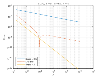
(a) BDF2 scheme for ODEs

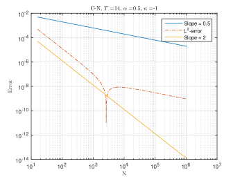
(b) C-N scheme for ODEs

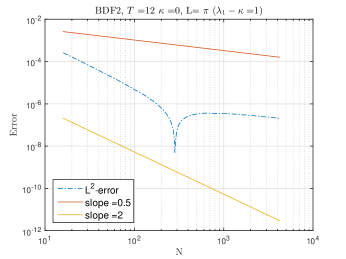
(c) BDF2 scheme for PDEs

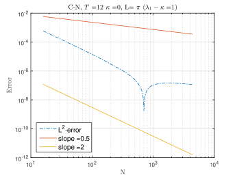
(d) C-N scheme for PDEs

Figure 1: Errors with fixed model parameters $T,\kappa,\lambda_{1}$: absolute error for ODEs and PDEs.

4.2 Conjecture and numerical experiments for sub-diffusion equations

It is known that the solution to the sub-diffusion equation (1.1) exhibits weak regularity (1.2) even for smooth initial values. As displayed in Table 1, various convergence rates of the $L1$ scheme are observed. Therefore, it is both significant and desirable to formulate corresponding decay-preserving estimates for the L1 scheme applied to equation (1.1).

Let $U^{n}$ be the numerical approximation to $u(x,t_{n})$. The L1 formula [12, 18, 9] for approximating the fractional Caputo derivative is defined as follws:

$$\mathcal{D}_{\tau}^{\alpha}U^{n}:=\frac{\tau^{-\alpha}}{\Gamma(2-\alpha)}\sum_{j=1}^{n}A_{n-j}(U^{j}-U^{j-1}),$$ (4.6)

where $A_{i}=(i+1)^{1-\alpha}-i^{1-\alpha}$. Hence, the semi-discrete L1 scheme to (1.2) is given by

$$\mathcal{D}_{\tau}^{\alpha}U^{n}=\Delta U^{n}+\kappa U^{n}+f^{n},$$ (4.7)

with $U^{0}(x)=u_{0}(x)$ and $U^{n}(x)=0,\;\forall x\in\partial\Omega$.

Due to the nonlocality of the fractional operator, obtaining a decay-preserving estimate poses an essential challenge, as the discrete fundamental solution to $\mathcal{D}_{\tau}^{\alpha}U^{n}=\kappa U^{n}$ is difficult to explicitly formulate. Therefore, we only propose a convincing conjecture regarding the decay-preserving estimate of the L1 scheme for sub-diffusion equations (1.1) and substantiate our conjecture numerically. The following conjecture is inspired by the error estimates for ODEs and PDEs and the fundamental solution of the following fractional ordinary equation

$$\partial_{t}^{\alpha}y(t)=\kappa y(t)+f(t),\quad y(0)=y_{0},$$

for example, see [1, Remark 7.1], which can be expressed in the form of

$$y(t)=y_{0}E_{\alpha}(\kappa t^{\alpha})+\alpha\int_{0}^{t}E_{\alpha}^{\prime}(\kappa(t-s)^{\alpha})(t-s)^{\alpha-1}f(s){\;\rm{d}}s.$$

Here $E_{\alpha}(\cdot):=\sum_{j=0}^{\infty}\frac{(\cdot)^{j}}{\Gamma(j\alpha+1)}$ represents Mittag-Leffler function [1]. The decay-preserving error estimate for the $L1$ scheme (4.7) is shown as follows.

Conjecture 4.1.

Let $u^{n}$ and $U^{n}$ be the solutions to (1.1) and the $L1$ scheme (4.7), respectively. Let $\lambda_{1}$ be the minimal eigenvalue of the eigenvalue problem (3.1), and let $\kappa<\lambda_{1}$. Then for sufficiently small $\tau$, ithe following holds:

$$\|e^{n}\|\leq E_{\alpha}(-C(\lambda_{1}-\kappa)t_{n}^{\alpha})\|e^{0}\|+C_{u,\alpha}t_{n}^{\alpha-1}\Big{(}E_{\alpha}^{\prime}(-C(\lambda_{1}-\kappa)t_{n}^{\alpha})\tau+\tau^{2-\alpha}\Big{)}.$$ (4.8)

Taking $e^{0}=0$ in (4.8), the error estimates at final time level $t_{N}=N\tau(=T)$ can be expressed as

$$\|e^{N}\|\leq C(E_{\alpha}^{\prime}(-C(\lambda_{1}-\kappa)T^{\alpha})\tau+\tau^{2-\alpha}).$$ (4.9)

It follows from (4.9) that the coefficient $E_{\alpha}^{\prime}(-C(\lambda_{1}-\kappa)T^{\alpha})$ of $\tau$ is decreasing with respect to $T$ when $\lambda_{1}>\kappa$ and is increasing when $\lambda_{1}\leq\kappa$. As discussed in the previous subsection, the trade-off or competition between the two scales $\mathcal{O}(E_{\alpha}^{\prime}(-C(\lambda_{1}-\kappa)T^{\alpha})\tau^{\alpha})$ and $\mathcal{O}(\tau^{2-\alpha})$ in (4.2) is the main cause of various convergence rate regimes. Therefore, we present a similar qualitative analysis as in (4.9) as follows.

• Case 1: $\kappa\geq\lambda_{1}.$ In this situation, the coefficient $E_{\alpha}^{\prime}(-C(\lambda_{1}-\kappa)T^{\alpha})$ increases with respect to $T$, making the first term $E_{\alpha}^{\prime}(-C(\lambda_{1}-\kappa)T^{\alpha})\tau$ in (4.9) consistently dominant. Consequently, the convergence rate for $\kappa\geq\lambda_{1}$ always behaves as first-order, i.e., $\mathcal{O}(\tau)$.

• Case 2: $\kappa<\lambda_{1}.$ In this situation, the coefficient $E_{\alpha}^{\prime}(-C(\lambda_{1}-\kappa)T^{\alpha})$ will decay with respect to $T$. Consequently, the convergence order can be qualitatively illustrated as follows:

  • Given a lower bound on the time steps $\tau_{0}$ and letting $\tau\geq\tau_{0}$, then

    1. for sufficiently small $\lambda_{1}-\kappa$ (relatively large $\kappa$ or small $\lambda_{1}$) and $T$, the convergence order is $\mathcal{O}(\tau)$;

    2. for sufficiently large $\lambda_{1}-\kappa$ (relatively small $\kappa$ or large $\lambda_{1}$) and $T$, the convergence order is $\mathcal{O}(\tau^{2-\alpha})$.

  • Given the model parameters $\kappa,\lambda_{1}$, and $T$, then

    1. for sufficiently small $\tau$, the convergence order is $\mathcal{O}(\tau)$.

Example 4.3.

We illustrate various convergence orders in different model parameter regimes using the $L1$ scheme (4.7). We follow the setting of space in Example 4.2, including the notations and definitions, and also use the benchmark solution of the sub-diffusion equation (1.1) constructed in (1.3), i.e., $u=t^{\alpha}\sin(\pi x/L)$. The convergence rates of the $L1$ scheme (4.7) are shown in Table 10 by fixing $T=1,L=\pi$, and decreasing $\kappa$, in Table 11 by fixing $\kappa=0,T=10$, and increasing $L$ and $N$, in Table 12 by fixing $\kappa=0,L=\pi$, and increasing the final time $T$, and in Table 13 by fixing $T=5$, $\kappa=1,1.5,L=\pi,4$, and increasing $N$.

As observed in Tables 10, 11 and 12, the convergence rates change from $\mathcal{O}(\tau)$ to $\mathcal{O}(\tau^{2-\alpha})$ as $\lambda_{1}$ and $T$ increase or $\kappa$ decreases, consistent with conclusions (E1) and (E2). Additionally, the convergence rates demonstrate a monotonous change, implying our Conjecture 4.1 is reasonable and effective in revealing the influence of the model parameters on the convergence orders of the $L1$ scheme.

For some choices of model parameters in Tables 10, 11 and 12, the convergence rates tend towards $\mathcal{O}(\tau)$ as $N$ increases, aligning with conclusion (E3). Table 13 illustrates that the convergence rate remains $\mathcal{O}(\tau)$ as long as $\kappa\geq\lambda_{1}$, consistent with our theoretical analysis in Case 1 for $\kappa\geq\lambda_{1}$.

We point out that the decay rate of Mittag-Leffler function is less than that of the exponential function. Therefore, to attain the optimal convergence order, the range of model parameters shall be chosen wider than in the previous subsection. As predicted, a broader range of model parameters, such as $\kappa=-50,T=100$, is selected in Tables 10, 11, and 12, in comparison to model parameters $|\kappa|\leq 20,T\leq 20$ in Tables 6, 7, and 8.

Table 10: (Example 4.3 for subdiffusion equation) Convergence rate with $T=1,L=\pi$ and various $\kappa$.

  $N$ $\kappa=0$ $\kappa=-5$ $\kappa=-10$ $\kappa=-20$ $\kappa=-50$ 64 1.06 1.23 1.31 1.38 1.44 128 1.05 1.19 1.26 1.34 1.42 256 1.03 1.15 1.22 1.30 1.39 512 1.02 1.11 1.18 1.25 1.36  

Table 11: (Example 4.3 for subdiffusion equation) Convergence rate with $\kappa=0,T=10$ and various $L$.

  $N$ $L=1$ $L=2$ $L=3$ $L=4$ $L=5$ $(\lambda_{1}\approx 9.87)$ $(\lambda_{1}\approx 2.47)$ $(\lambda_{1}\approx 1.10)$ $(\lambda_{1}\approx 0.62)$ $(\lambda_{1}\approx 0.39)$ 64 1.41 1.26 1.17 1.11 1.08 128 1.38 1.22 1.13 1.08 1.06 256 1.34 1.18 1.10 1.06 1.04 512 1.31 1.14 1.07 1.04 1.03  

Table 12: (Example 4.3 for subdiffusion equation) Convergence rate with $\kappa=0,L=\pi$ and various $T$.

  $N$ $T=1$ $T=10$ $T=20$ $T=50$ $T=100$ 64 1.06 1.16 1.20 1.25 1.30 128 1.05 1.12 1.15 1.21 1.25 256 1.03 1.09 1.12 1.17 1.21 512 1.02 1.07 1.09 1.13 1.17  

Table 13: (Example 4.3 for subdiffusion equation) Convergence rate with $T=5,\kappa\geq\lambda_{1}$ and various $L$.

  $N$ $\kappa=1$ $\kappa=1.5$ $L=\pi$ $L=4$ $L=\pi$ $L=4$ $(\lambda_{1}=1)$ $(\lambda_{1}\approx 0.62)$ $(\lambda_{1}=1)$ $(\lambda_{1}\approx 0.62)$ 64 1.00 0.94 0.92 0.92 128 1.00 0.96 0.94 0.92 256 1.00 0.97 0.96 0.93 512 1.00 0.98 0.97 0.95  

5 Detailed proofs for the main results

5.1 The proof of Theorem 2.3

Since BDF2 is a two-step method, the analysis of decaying errors is more chanllenging than for the Euler and C-N schemes. Here, we introduce the concept of a discrete orthogonal convolution (DOC) kernel, which differs from the BDF2 convolution kernels provided in [11, 21].

Definition 5.1.

For convolution sequence $\{A^{(n)}_{n-k}\}_{k=1}^{n}$, the DOC kernel in [11] is defined by

$$\sum_{j=k}^{n}\theta_{n-j}^{(n)}A_{j-k}^{(j)}\equiv\delta_{nk},\quad\forall 1\leq k\leq n,$$ (5.1)

where $\delta_{nk}$ denotes the Kronecker delta symbol with $\delta_{nk}=1$ if $n=k$ and $\delta_{nk}=0$ if $n\neq k$.

Lemma 5.1.

Let $0<-\kappa\tau<1/2$ and the BDF2 kernels $A_{n-k}^{(n)}$ defined by (2.31). Then the DOC kernels defined by (5.1) can be explicitly expressed as

$$\theta^{(n)}_{n-1} =\frac{2-2\kappa\tau}{3-2\kappa\tau}\frac{1}{\sqrt{1+2\kappa\tau}}\big{(}(2-\sqrt{1+2\kappa\tau})^{-n}-(2+\sqrt{1+2\kappa\tau})^{-n}\big{)},$$ (5.2)

$$\theta^{(n)}_{n-k} =\frac{1}{\sqrt{1+2\kappa\tau}}\big{(}(2-\sqrt{1+2\kappa\tau})^{-(n-k+1)}-(2+\sqrt{1+2\kappa\tau})^{-(n-k+1)}\big{)}.$$ (5.3)

Proof. Form the definition of the DOC kernels (5.1), one has

$$\theta^{(n)}_{0}A^{(n)}_{0} =1,$$

$$\theta^{(n)}_{0}A^{(n)}_{1}+\theta^{(n)}_{1}A^{(n-1)}_{0} =0,$$

$$\theta^{(n)}_{n-j}A^{(j)}_{0}+\theta^{(n)}_{n-j-1}A^{(j+1)}_{1}+\theta^{(n)}_{n-j-2}A^{(j+2)}_{2} =0,\quad j\leq n-2.$$

Set $a_{j}:=\theta^{(n)}_{n-j}A^{(j)}_{0}\;(1\leq j\leq n)$ and $\phi:=(3/2-\kappa\tau)^{-1}$. Then $a_{j}$ solves

$$a_{n}=1,\quad a_{n-1}=2\phi,\quad a_{j}=2\phi a_{j+1}-\frac{1}{2}\phi a_{j+2}\;(j\leq n-2),$$

where the definition (2.31) is used. It is easy to check $\phi\in(\frac{1}{2},\frac{2}{3})$ by the fact $0<-\kappa\tau<\frac{1}{2}$. Let $c=-\phi-\sqrt{\phi(\phi-\frac{1}{2})}$ be the solution to equation $x^{2}+2\phi x+\phi/2=0$ and $b=c+2\phi$. Then for $j\leq n-2$, one finds

$$a_{j}+ca_{j+1}=b(a_{j+1}+ca_{j+2})=\cdots=b^{n-j-1}(a_{n-1}+ca_{n})=b^{n-j}.$$ (5.4)

Let $d=-\frac{b}{b+c}$. It is easy to verify that (5.4) can be reformulated into

$$\frac{a_{j}}{b^{n-j}}+d=(-\frac{c}{b})(\frac{a_{j+1}}{b^{n-j-1}}+d)=\cdots=(-\frac{c}{b})^{n-1-j}(\frac{a_{n-1}}{b}+d).$$

Thus, we finally arrive at

$$a_{j}=-\frac{1}{b+c}\big{(}(-c)^{n-j+1}-b^{n-j+1}\big{)},$$

where $b=2\phi+c=\frac{1}{2+\sqrt{1+2\kappa\tau}}$ and

$$-c=\phi+\sqrt{\phi(\phi-\frac{1}{2})}=\frac{\phi/2}{\phi-\sqrt{\phi(\phi-\frac{1}{2})}}=\frac{1}{2-\sqrt{4-2/\phi}}=\frac{1}{2-\sqrt{1+2\kappa\tau}}.$$

The proof is completed by the identity $\theta^{(n)}_{n-j}:=a_{j}/A^{(j)}_{0}(1\leq j\leq n)$.  

With the help of the new DOC kernels, Theorem 2.3 can be proven as follows.

Proof of Theorem 2.3
Proof. Multiplying Eq. (2.32) by the DOC kernels and summing over $k$, one has

$$\sum_{k=1}^{n}\theta^{(n)}_{n-k}\sum_{j=1}^{k}A^{(n)}_{n-k}e^{j}=\sum_{k=1}^{n}\theta^{(n)}_{n-k}\tau R^{k}.$$ (5.5)

Applying the definition of DOC kernels (5.1) to the left hand, one finds

$$\sum_{k=1}^{n}\theta^{(n)}_{n-k}\sum_{j=1}^{k}A^{(n)}_{n-j}e^{j}=\sum_{j=1}^{n}e^{j}\sum_{k=j}^{n}\theta^{(n)}_{n-k}A^{(n)}_{n-j}=e^{n}.$$ (5.6)

Hence, we arrive at

$$e^{n}=\sum_{k=1}^{n}\theta^{(n)}_{n-k}\tau R^{k}=\sum_{k=1}^{n}\theta^{(n)}_{n-k}\tau\eta^{k}+(\theta^{(n)}_{n-2}/2-\theta^{(n)}_{n-1})e^{0},$$ (5.7)

where (2.33) is used. It is easy to check

$$(2-\sqrt{1+2\kappa\tau})^{-(n-k+1)}=(1-\frac{2\kappa\tau}{1+\sqrt{1+2\kappa\tau}})^{-(n-k+1)}\leq(1-\kappa\tau)^{-(n-k+1)}.$$

Then for $\tau<1/(4\lambda)$, combining with Lemma 5.1, one produces

$$0<\theta^{(n)}_{n-k}\leq 2(1-\kappa\tau)^{-(n-k+1)}.$$ (5.8)

Inserting the inequality (5.8) into (5.7), one yields

$$|e^{n}|\leq (1-\kappa\tau)^{-n}|e^{0}|+2\sum_{k=1}^{n}\tau(1-\kappa\tau)^{-(n-k+1)}|\eta^{k}|$$

$$\leq (1-\kappa\tau)^{-n}|e^{0}|+2C_{u,\alpha}\big{(}\sum_{k=2}^{n-2}\tau^{3}(1-\kappa\tau)^{-(n-k-1)}t_{k}^{\alpha-3}+4(1-\kappa\tau)^{-n}\tau^{\alpha}\big{)},$$

where the last inequality uses estimates in (2.34) and the fact $\tau\leq 1/(-4\kappa)$.

Set $\rho_{\tau}=(1-\kappa\tau)$ and $S_{n}=\sum_{k=2}^{n-2}\tau\rho_{\tau}^{-(n-k-1)}t_{k}^{\alpha-3}$. Then, we has

$$|e^{n}|\leq\rho_{\tau}^{-n}|e^{0}|+2C_{u,\alpha}\Big{(}S_{n}\tau^{2}+4\rho_{\tau}^{-n}\tau^{\alpha}\Big{)}.$$ (5.9)

It follows from Lemma 2.1 that

$$S_{n} \leq\frac{1}{2-\alpha}\Big{(}(2^{2-\alpha}(1-\rho_{\tau}^{-(\frac{n}{2}-1)})-1)t_{n-1}^{\alpha-2}+\rho_{\tau}^{-(\frac{n}{2}-2)}\tau^{\alpha-2}\Big{)}.$$ (5.10)

Applying Lemma 2.2 to (5.10) and noting $\rho_{\tau}^{2}\leq 2$, one has

$$S_{n} \leq\frac{1}{2-\alpha}\Big{(}(2^{2-\alpha}(1-e^{\frac{\kappa t_{n}}{2}})-1)t_{n-1}^{\alpha-2}+2e^{\frac{\kappa t_{n}}{4}}\tau^{\alpha-2}\Big{)}.$$ (5.11)

Thus, the proof is completed by inserting (5.11) into (5.9) and using Lemma 2.2.  

5.2 The proofs of the main results in Section 3

The following lemma will be widely used in the proofs.

Lemma 5.2.

We here present the following discrete and continuous estimates:

1. Let $\bm{a}=(a_{k})_{k=1}^{\infty},\bm{b}^{j}=(b_{k}^{j})_{k=1}^{\infty}\in l^{2},\;1\leq j\leq m$ for some positive integers $m$. If $a_{k}\leq\sum_{j=1}^{m}b_{k}^{j}$ for all $1\leq k<\infty$, then it holds that

   $$\sqrt{\sum_{k=1}^{\infty}a_{k}^{2}}\leq\sum_{j=1}^{m}\sqrt{\sum_{k=1}^{\infty}(b_{k}^{j})^{2}}.$$ (5.12)

2. Let $v_{k}(x)\in L^{2}((a,b)),1\leq k<\infty$ for some fixed interval $(a,b)$. Assume there exists $v^{*}(x)\in L^{2}((a,b))$ such that the series $\sum_{k=1}^{\infty}v_{k}^{2}(x)\leq v^{*}(x),a.e.$. Then, it holds that

   $$\sum_{k=1}^{\infty}(\int_{a}^{b}v_{k}(s){\;\rm{d}}s)^{2}\leq(\int_{a}^{b}\sqrt{\sum_{k=1}^{\infty}v_{k}^{2}(s)}{\;\rm{d}}s)^{2}.$$ (5.13)

Proof. Note that the $l^{2}$-norm is given by $\|\bm{\upsilon}\|_{l^{2}}=\sqrt{\sum_{k=1}^{\infty}(\upsilon_{k})^{2}}$ for all $\bm{\upsilon}=(\upsilon_{k})_{k=1}^{\infty}\in l^{2}$. Thus, the first claim can be immediately derived by the triangle inequality of $l^{2}$-norm and the assumption $a_{k}\leq\sum_{j=1}^{m}b_{k}^{j}$. Note that

$$\sum_{k=1}^{n}(\int_{a}^{b}v_{k}(s){\;\rm{d}}s)^{2} =\int_{a}^{b}\int_{a}^{b}(\sum_{k=1}^{n}v_{k}(s)v_{k}(r)){\;\rm{d}}s{\;\rm{d}}r$$

$$\leq\int_{a}^{b}\int_{a}^{b}\sqrt{\sum_{k=1}^{n}v_{k}^{2}(s)}\sqrt{\sum_{k=1}^{n}v_{k}^{2}(r)}{\;\rm{d}}s{\;\rm{d}}r$$

$$=(\int_{a}^{b}\sqrt{\sum_{k=1}^{n}v_{k}^{2}(s)}{\;\rm{d}}s)^{2}.$$

The proof of the second claim is completed by taking $n\to\infty$ and using the dominated convergence theorem.  

The proof of Theorem 3.1
Proof. From (3.2), the solutions to (1.4) and (3.4) has the following representations

$$u=\sum_{k=1}^{\infty}d_{k}(t)\omega_{k}(x),$$ (5.14)

$$U^{n}=\sum_{k=1}^{\infty}d_{k}^{n}\omega_{k}(x),$$ (5.15)

where $d_{k}(t)=(u,\omega_{k})$ and $d_{k}^{n}=(U^{n},\omega_{k})$. Taking inner products of (3.5) with $\omega_{k}$ yields

$$\nabla_{\tau}e_{k}^{n} =-(\lambda_{k}-\kappa)\tau e_{k}^{n}+\tau R^{n},$$ (5.16)

where $e_{k}^{n}:=d_{k}(t_{n})-d_{k}^{n}$, $R^{n}_{k}=-\frac{1}{\tau_{n}}\int_{t_{n-1}}^{t_{n}}(s-t_{n-1})\partial_{tt}d_{k}(s){\;\rm{d}}s$ and $\lambda_{k}$ is the eigenvalue of eigenvalue problem (3.1). Applying Lemma 5.2 to (5.16), we arrive at

$$\sqrt{\sum_{k=1}^{\infty}(1+(\lambda_{k}-\kappa)\tau)^{2}|e_{k}^{n}|^{2}}\leq\sqrt{\sum_{k=1}^{\infty}|e_{k}^{n-1}|^{2}}+\tau\sqrt{\sum_{k=1}^{\infty}|R_{k}^{n}|^{2}}.$$ (5.17)

Note that $\|u\|^{2}=\sum_{k=1}^{\infty}|d_{k}|^{2}$ and $\|e^{n}\|^{2}=\sum_{k=1}^{\infty}|e^{n}_{k}|^{2}$. Applying Lemma 5.2 again to the last term of (5.17), one has

$$\sqrt{\sum_{k=1}^{\infty}|R_{k}^{n}|^{2}}\leq\frac{1}{\tau_{n}}\int_{t_{n-1}}^{t_{k}}(s-t_{n-1})\|u_{tt}\|{\;\rm{d}}s:=\hat{R}^{n}.$$ (5.18)

Hence, we arrive at

$$(1+(\lambda_{1}-\kappa)\tau)\|e^{n}\|\leq\|e^{n-1}\|+\tau\hat{R}^{n},$$ (5.19)

which implies

$$\|e^{n}\|\leq(1+(\lambda_{1}-\kappa)\tau)^{-n}\|e^{0}\|+\tau\sum_{k=1}^{n}(1+(\lambda_{1}-\kappa)\tau)^{-(n+1-k)}\hat{R}^{k}.$$ (5.20)

The remaining proof is similar to that of Theorem 2.1, and we omit it here.  

The proof of Theorem 3.2
Proof. Taking inner products of (3.8) with $\omega_{k}$, one has

$$(1+\frac{\lambda_{k}-\kappa}{2}\tau)e_{k}^{n}=(1-\frac{\lambda_{k}-\kappa}{2}\tau)e_{k}^{n-1}+R_{k}^{n},$$ (5.21)

where $R_{k}^{n}:=(R^{n},\omega)$ and $R^{n}=R_{1}^{n}+R_{2}^{n}$. It follows from (5.14), (5.15) that

$$\|e^{n}\|=\sum_{k=1}^{\infty}|e_{k}^{n}|^{2}.$$

Note that $\|u\|^{2}=\sum_{k=1}^{\infty}d_{k}(t)^{2}$, then from (3.9), (3.10), (5.12) and (5.13), one finds

$$\sqrt{\sum_{n=1}^{\infty}|R_{k}^{n}|^{2}}\leq\hat{R}^{n}.$$ (5.22)

For simplicity of notation, denote by $\psi_{k}:=\frac{1+\frac{(\lambda_{k}-\kappa)\tau}{2}}{1-\frac{(\lambda_{k}-\kappa)\tau}{2}}$. Then, we arrive at

$$|e_{k}^{n}|\leq\psi_{k}^{-n}|e_{k}^{0}|+\tau(1+\frac{(\lambda_{k}-\kappa)\tau}{2})^{-1}\sum_{j=1}^{n}\psi_{j}^{-(n-j)}R_{k}^{j}.$$ (5.23)

Squaring both sides and summing $k$ from 1 to $\infty$, it follows from (5.12) that

$$\|e^{n}\|\leq\psi_{1}^{-n}\|e^{0}\|+\tau(1+\frac{(\lambda_{1}-\kappa)\tau}{2})^{-1}\sum_{j=1}^{n}\psi_{1}^{-(n-j)}\hat{R}^{j},$$ (5.24)

where $\hat{R}^{j}$ satisfies (3.13). The rest proof is similar to the proof of Theorem 2.2 and we omit here.  

The proof of Theorem 3.3
Proof. Taking inner products of both sides with $\omega_{k}$, one has

$$e_{k}^{1}-e_{k}^{0} =-(\lambda_{k}-\kappa)\tau e_{k}^{1}+\tau\eta_{k}^{1}, x\in\Omega,\;$$ (5.25)

$$\frac{3}{2}e_{k}^{n}-2e_{k}^{n-1}+\frac{1}{2}e_{k}^{n-2} =-(\lambda_{k}-\kappa)\tau e_{k}^{n}+\tau\eta_{k}^{n}, x\in\Omega,\;2\leq n\leq N,$$ (5.26)

where $e_{k}^{n}:=d_{k}(t_{n})-d_{k}^{n}$, $\eta^{n}_{k}=(\eta^{n},\omega_{k})$ and $\lambda_{k}$ is the eigenvalue of eigenvalue problem (3.1). It follows from (5.14), (5.15) that

$$\|e^{n}\|= \sum_{k=1}^{\infty}|e_{k}^{n}|^{2}.$$ (5.27)

Denote by $\hat{\eta}^{n}:=\sum_{n=1}^{\infty}|\eta_{k}^{n}|^{2}$. Similar to (5.22), from (5.12), (5.13) and assumption (1.2), one has

$$\hat{\eta}^{n} \leq C_{u,\alpha}t_{k-2}^{\alpha-3}\tau^{2},\quad\;n\geq 3$$ (5.28)

$$\hat{\eta}^{n} \leq C_{u,\alpha}\tau^{\alpha-1},\qquad n=1,2.$$ (5.29)

Set $R_{k}^{l}=\eta_{k}^{l}(l\geq 3)$ and $R_{k}^{2}=\eta_{k}^{2}-\frac{e_{k}^{0}}{2\tau},\;R_{k}^{1}=\eta_{k}^{1}+\frac{e_{k}^{0}}{\tau}$. We further introduce the following notations, say the BDF2 kernels, as $A^{(k,1)}_{0}:=1+(\lambda_{k}-\kappa)\tau$ and for $l\geq 2$

$$A^{(k,l)}_{0}:=\frac{3}{2}+(\lambda_{k}-\kappa)\tau,\;A^{(k,l)}_{1}:=-2,\;A^{(k,l)}_{2}:=\frac{1}{2},\;A^{(k,l)}_{j}=0,\quad j\geq 3.$$

The error identities (5.25) and (5.26) may be refined as a convolution form

$$\sum_{j=1}^{l}A^{(k,l)}_{l-j}e_{k}^{j}=R_{k}^{l}.$$ (5.30)

Let $\theta^{(k,n)}_{n-j}$ be the DOC kernels corresponding to the BDF2 kernels $A^{(k,n)}_{n-j}$. Multiplying both sides of (5.30) by the DOC kernels $\theta^{(k,n)}_{n-j}$ and summing over $j$, one has

$$e_{k}^{n}=\sum_{j=1}^{n}\theta^{(k,n)}_{n-j}\tau R_{k}^{j}=\sum_{j=1}^{n}\theta^{(k,n)}_{n-j}\tau\eta_{k}^{j}+(\theta^{(k,n)}_{n-2}/2-\theta^{(k,n)}_{n-1})e_{k}^{0}.$$ (5.31)

Similar to (5.8), for $\tau<1/(4(\lambda_{k}-\kappa))$, the DOC kernels satisfy

$$0<\theta^{(k,n)}_{n-j}\leq 2(1+(\lambda_{k}-\kappa)\tau)^{-(n-j+1)}\leq 2(1+(\lambda_{1}-\kappa)\tau)^{-(n-j+1)}.$$ (5.32)

Inserting (5.32) into (5.31), one arrive at

$$|e_{k}^{n}|\leq(1+(\lambda_{1}-\kappa)\tau)^{-n}|e_{k}^{0}|+2\sum_{j=1}^{n}\tau(1+(\lambda_{1}-\kappa)\tau)^{-(n-j+1)}|\eta_{k}^{j}|.$$ (5.33)

Squaring both sides and summing from 1 to $\infty$, combining with (5.12), (5.27)-(5.29), one has

$$\|e^{n}\|\leq(1+(\lambda_{1}-\kappa)\tau)^{-n}\|e^{0}\|+2\sum_{j=1}^{n}\tau(1+(\lambda_{1}-\kappa)\tau)^{-(n-j+1)}\hat{\eta}^{j}.$$ (5.34)

The rest proof is similar to the proof of Theorem 3.3 and we omit here.  

6 Conclusion

When employing popular numerical schemes to solve diffusion and subdiffusion equations with weakly initial singularity (1.2), various convergence orders can be observed. In this paper, we introduce a general methodology and propose a new decay-preserving error estimate to systematically analyze the numerical behavior of widely used IE, C-N and BDF2 schemes. The decay-preserving error estimate comprises two components: $e^{-C(\lambda_{1}-\kappa)T}\tau^{\alpha}$ and $T^{\alpha-k}\tau^{k}$, where $\lambda_{1}$ is the minimal eigenvalue of the problem (3.1). This estimate reveals that the diverse convergence rates arise due to the trade-off between these two components in different model parameter regimes. Our decay-preserving error estimates successfully capture varying convergence states, overcoming limitations of traditional error estimates by incorporating model parameters, retaining more properties of continuous equations. Furthermore, we present a conjecture regarding the decay-preserving error estimate of the L1 scheme for sub-diffusion equations (1.1). This conjecture sheds light on the phenomena where the L1 scheme may exhibit different convergence rates in distinct model parameter regimes. We provide numerical results to validate our analysis.

Nevertheless, our decay-preserving error estimates may not account for certain numerical phenomena, such as the observed kinks in the convergence rate transition from high-order to low-order as depicted in Figure 1. This suggests the possibility of a sup-convergence point $N_{0}$ where the $L^{2}$-norm errors experience a dramatic drop. Consequently, a more sophisticated estimate is needed to interpret these intriguing phenomena in the future.

References

- [1] K. Diethelm. The analysis of fractional differential equations: An application-oriented exposition using differential operators of caputo type. Springer Berlin, Heidelberg, 2010.
- [2] J. Gracia, E. O’Riordan, and M. Stynes. Convergence in positive time for a finite difference method applied to a fractional convection-diffusion problem. Comput. Meth. Appl. Mat., 18(1):33–42, 2018.
- [3] B. Jin, R. Lazarov, and Z. Zhou. An analysis of the L1 scheme for the subdiffusion equation with nonsmooth data. IMA J. Numer. Anal., 36(1):197–221, 2016.
- [4] B. Jin, B. Li, and Z. Zhou. Correction of high-order bdf convolution quadrature for fractional evolution equations. SIAM J. Sci. Comput., 39(6):A3129–A3152, 2017.
- [5] B. Jin, B. Li, and Z. Zhou. Numerical analysis of nonlinear subdiffusion equations. SIAM J. Numer. Anal., 56(1):1–23, 2018.
- [6] J. Klafter and I. Sokolov. First steps in random walks: from tools to applications. OUP Oxford, 2011.
- [7] N. Kopteva. Error analysis of an L2-type method on graded meshes for a fractional-order parabolic problem. Math. Comp., 90(327):19–40, 2021.
- [8] D. Li, H. Qin, and J. Zhang. Sharp pointwise-in-time error estimate of L1 scheme for nonlinear subdiffusion equations. 2021. arXiv preprint arXiv:2101.04554.
- [9] H. Liao, D. Li, and J. Zhang. Sharp error estimate of the nonuniform L1 formula for linear reaction-subdiffusion equations. SIAM J. Numer. Anal., 56(2):1112–1133, 2018.
- [10] H. Liao, W. McLean, and J. Zhang. A discrete gronwall inequality with applications to numerical schemes for subdiffusion problems. SIAM J. Numer. Anal., 57(1):218–237, 2019.
- [11] H. Liao and Z. Zhang. Analysis of adaptive BDF2 scheme for diffusion equations. Math. Comp., 90(329):1207–1226, 2020.
- [12] Y. Lin and C. Xu. Finite difference/spectral approximations for the time-fractional diffusion equation. J. Comput. Phys., 225(2):1533–1552, 2007.
- [13] C. Lubich. Convolution quadrature and discretized operational calculus. I. Numer. Math., 52(2):129–145, 1988.
- [14] W. McLean and K. Mustapha. Time-stepping error bounds for fractional diffusion problems with non-smooth initial data. J. Comput. Phys., 293:201–217, 2015.
- [15] R. Metzler, J. Jeon, A. Cherstvy, and E. Barkai. Anomalous diffusion models and their properties: non-stationarity, non-ergodicity, and ageing at the centenary of single particle tracking. Phys. Chem. Chem. Phys., 16(44):24128–24164, 2014.
- [16] R. Metzler and J. Klafter. The random walk’s guide to anomalous diffusion: a fractional dynamics approach. Phys. Rep., 339(1):1–77, 2000.
- [17] M. Stynes, E. O’Riordan, and J.L. Gracia. Error analysis of a finite difference method on graded meshes for a time-fractional diffusion equation. SIAM J. Numer. Anal., 55:1057–1079, 2017.
- [18] Z. Sun and X. Wu. A fully discrete scheme for a diffusion wave system. Appl. Numer. Math., 56(2):193–209, 2006.
- [19] V. Thomée. Galerkin finite element methods for parabolic problems, second edition. Springer Berlin, Heidelberg, 2006.
- [20] Y. Yan, M. Khan, and N. Ford. An analysis of the modified L1 scheme for time-fractional partial differential equations with nonsmooth data. SIAM J. Numer. Anal., 56(1):210–227, 2018.
- [21] J. Zhang and C. Zhao. Sharp error estimate of BDF2 scheme with variable time steps for linear reaction-diffusion equations. J. Math., 41(6):471–488, 2021.