The exponential turnpike property for periodic linear quadratic optimal control problems in infinite dimension 111This work was partially supported by the National Natural Science Foundation of China under the grant 11971363, and by the Fundamental Research Funds for the Central Universities under the grant 2042023kf0193.
Abstract
In this paper, we establish an exponential periodic turnpike property for linear quadratic optimal control problems governed by periodic systems in infinite dimension. We show that the optimal trajectory converges exponentially to a periodic orbit when the time horizon tends to infinity. Similar results are obtained for the optimal control and adjoint state. Our proof is based on the large time behavior of solutions of operator differential Riccati equations with periodic coefficients.
keywords:
Periodic turnpike , periodic Riccati equation , exponential stabilityMSC:
[2010] 49J20, 49K20, 93D201 Introduction
The turnpike property was first observed in the context of finite-dimensional discrete-time optimal growth problems by economists (see, e.g., [9, 20]). This property reflects the fact that, for an optimal control problem for which the time horizon is large enough, its optimal solution stays most of the time close to a turnpike set.
In many cases, the turnpike set is a singleton consisting of the minimizer of an optimal steady-state problem (see, e.g., [12, 13, 14, 15, 22, 29, 31, 32, 37]). But turnpike sets may be more complicated and may consist for instance of periodic orbits (see, e.g., [11, 29, 30]). In [24], Samuelson established a periodic turnpike property for a finite-dimensional optimal growth problem in economics, where the minimization functional is periodic in time. In [30, 36], the authors considered the periodic turnpike property in the context of dissipativity. In [25, 26], the authors established a turnpike property for finite-dimensional stochastic LQ optimal control problems.
The simplest time-varying linear systems are those for which the coefficients are time periodic. Periodic linear systems arise frequently as the result of linearizing a nonlinear system along a periodic orbit. In [35], the author established a characterization of periodic stabilization in terms of a detectability inequality for a linear periodic control system in a Hilbert space with a bounded control operator. The problem of tracking periodic signals for finite and infinite-dimensional linear periodic systems has been considered in [2] and [16].
The authors of [31] established a periodic turnpike property for linear quadratic (LQ) optimal control problems with periodic tracking terms for time-invariant systems under exponential stabilizability and detectability assumptions as well as some smallness assumptions. The main ingredient in [31] is a dichotomy transformation for the solutions of the algebraic Riccati and Lyapunov equations.
In the present paper we investigate the periodic exponential turnpike property for infinite-dimensional LQ optimal control problems with periodic coefficients, under appropriate periodic exponential stabilizability and detectability assumptions. The goal is to show that, except at the extremities of the time interval, the optimal trajectory (also, control and adjoint state) remains exponentially close to a periodic optimal trajectory, which itself is characterized as the optimal solution of an associated periodic optimal control problem. This widely generalizes the above-mentioned result of [31] and the technique of proof is entirely different.
Our approach here exploits the exponential stabilizability of the evolution operator resulting from the operator differential Riccati equation, and an exponential estimate between the solution of the differential Riccati equation with a zero terminal value to its periodic one, when the time horizon tends to infinity (see Proposition 3.1). This new exponential estimate is at the heart of the proof. The techniques that we use are inspired from earlier works by Da Prato and Ichikawa (see [6, 7, 8, 16]).
The paper is organized as follows. In Section 2, we introduce the LQ optimal control problem for periodic systems, and we state our main result, Theorem 2.1. In Section 3, we first establish some instrumental properties of the evolution operator resulting from the Riccati equation, and then we state and prove Proposition 3.1. Theorem 2.1 is proved in Section 4. Section 5 gives some further comments.
2 Main result
2.1 Formulation of the LQ optimal control problem
Throughout the paper, we use and to denote Hilbert spaces, and use and to denote the inner product and norm in all spaces without causing any confusion. We denote by the space of linear bounded operators from to . We set and , where denotes the adjoint operator of . We denote by the space of all mappings such that is continuous for any with the norm
Given any , we consider the time-periodic linear quadratic optimal control problem
where is -periodic, i.e. for every , and satisfies the controlled system
| (2.1) |
where , , and are -periodic, i.e. for every , and the same for the others. Here, for each , is a linear unbounded operator in , , , , and there exists such that for every .
Moreover, we assume that generates an evolution system, i.e., there exists a strongly continuous mapping such that
and there exists Yosida’s approximation for every , for large enough so that
Remark 2.1.
The conditions about the operators are fulfilled under the usual hypotheses of Tanabe and Kato-Tanabe (see, for instance, [1], [5], [17], [19], [21] and [27]). Sometimes, the strongly continuous mapping is called the evolution operator associated with . It can be noted that Yosida’s approximation is satisfied if, for instance, the family of is dissipative or quasi-dissipative (see, for instance, [17]), which is a standard assumption in that context. The existence of , the evolution operator associated with , is clear, since is bounded for each (see, for instance, [8]).
Remark 2.2.
The system has a unique mild solution given by
Moreover, the evolution operator is -periodic, i.e.,
The problem has a unique optimal solution denoted by .222The optimal solution depends on , and we add a superscript to emphasize this fact. Moreover, according to [18, Chapter 4, Theorem 1.6], there exists an adjoint state such that
| (2.2) |
in the mild sense along , with the two-point boundary condition
| (2.3) |
Furthermore, the optimal control is given by
2.2 The periodic turnpike theorem
In order to define the turnpike set, we consider the periodic optimal control problem:
over all pairs satisfying
| (2.4) |
The system does not necessarily have a periodic solution for a given -periodic control . This happens when no Floquet exponent of is equal to , i.e., when belongs to the resolvent set333The resolvent set of a closed linear operator is the set of all complex numbers such that the operator has a bounded inverse. of , or that is exponentially stable (see, for instance, [7, Proposition 2.1]). In fact, if belongs to the resolvent set , then the system has a unique mild solution for every -periodic control , given by
Actually, under some specific conditions, the exponentially stability of implies that belongs to the resolvent set of (see, for instance, [3, Corollary 2.1]).
Existence and uniqueness of a periodic solution for such periodic problems (Per)θ under certain conditions, as well as necessary and sufficient conditions for optimality, have been widely studied in the existing literature (see, for instance, [3], [6] or [18, Chapter 4, Proposition 5.2]). It is well known that if is an optimal pair for , then there exists an adjoint variable such that
| (2.5) |
in the mild sense along , with the periodic boundary conditions
| (2.6) |
Moreover, the optimal periodic control is given by
| (2.7) |
We say that is the periodic solution of (Per)θ.
In our main result (Theorem 2.1) hereafter, the assumptions that we do indeed ensure the existence and uniqueness of the periodic solution of (Per)θ, which is the turnpike set around which the exponential turnpike property is established. To introduce these assumptions, we next recall the definitions of exponential stabilizability and detectability in the time-periodic framework.
Definition 2.1.
The periodic pair is called exponentially -periodic stabilizable if there exists a feedback -periodic function such that the following closed-loop system is exponentially stable:
The periodic pair is called exponentially -periodic detectable if is exponentially -periodic stabilizable, i.e., there exists a feedback -periodic function such that the following closed-loop system is exponentially stable:
Theorem 2.1.
Assume that is exponentially -periodic stabilizable, and that is exponentially -periodic detectable. Then the problem has a unique solution (extended by -periodicity over the whole real line). Moreover, we have the exponential periodic turnpike property: there exist two positive constants and such that for any large enough, the optimal solution of satisfies
| (2.8) |
for every .
Remark 2.3.
The exponential decay constant in is the exponential stability rate for the evolution operator resulting from the operator Riccati equation in below, and the constant in is of the form , where the constant does not depend on and .
2.3 Examples
2.3.1 Periodic heat equation
Let be an open and bounded domain of with a boundary . Let be a non-empty open subset with its characteristic function . Given and , we consider the following optimal control problem:
| (2.9) |
subject to
where and are -periodic with respect to the time variable, and is the classical Laplace operator. The periodic optimal control problem (Per)θ reads as
| (2.10) |
subject to
We take = = , = = , = for each , and
Clearly, , and generates an evolution operator in . By [33, Corollary 2.1], is exponentially -periodic stabilizable, and is exponentially -periodic detectable. Therefore, according to Theorem 2.1, the periodic optimal control problem (Per)θ has a unique solution, and the optimal control problem under consideration has the periodic exponential turnpike property (2.8).
2.3.2 Periodic wave equation
Given , let be a 1-periodic tracking trajectory, i.e., for any . Given , we consider the following optimal control problem:
| (2.11) |
over all possible satisfying
where is -periodic with respect to the time variable, and .
We take . For each , define
where is the identity operator, and . There exist and such that and is exponentially stable (see, e.g., [7, Example 4.3]). Moreover note that , , and . Hence is exponentially -periodic stabilizable with and is exponentially -periodic detectable with . Therefore, according to Theorem 2.1, the optimal control problem under consideration has the periodic exponential turnpike property (2.8).
2.4 A numerical simulation
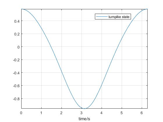
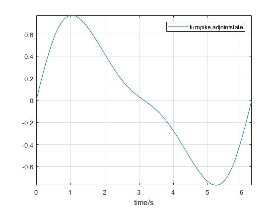
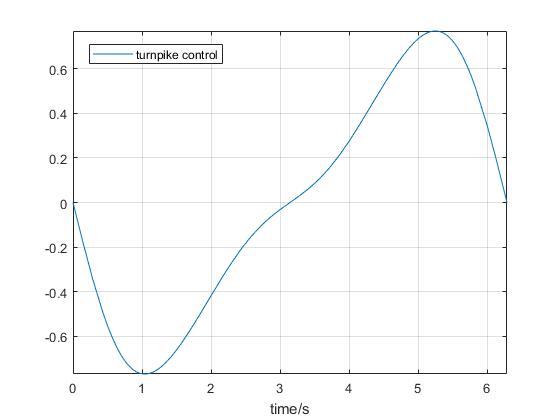
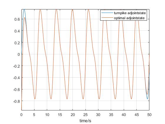
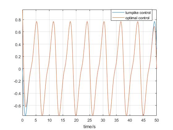
In this section, we provide a simple example to numerically illustrate the periodic turnpike phenomenon in the finite-dimensional case. Given any , we consider the LQ optimal control problem of minimizing the cost functional
for the one-dimensional control system
with a fixed initial condition .
To fit in our framework, we set for each
Using MATLAB,
-
1.
First, we compute the periodic solution of the periodic Riccati equation (3.2).
-
2.
Second, we compute the periodic solution of the equation (3.9).
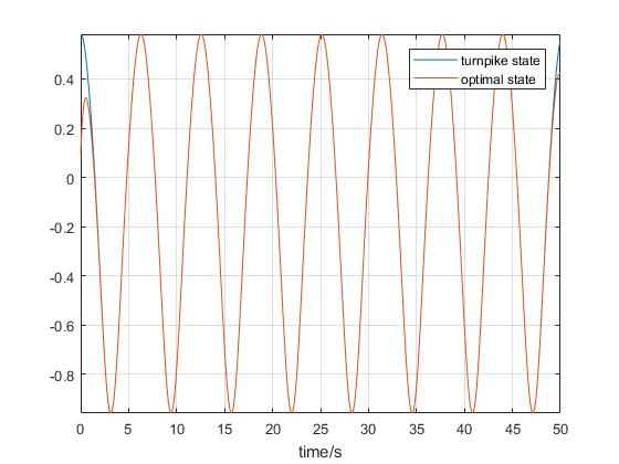
- 3.
The optimal extremal , resulting from the first-order optimality system derived from the Pontryagin maximum principle, can be computed in time , by the MATLAB function bvp4c. The turnpike property can be observed in the Figure 1 below. As expected, except for the transient initial and final arcs, the extremal (in red) remains close to the periodic turnpike (in blue).
3 Auxiliary results
3.1 Reminders on differential Riccati equations
We first state two preliminary results, see their proofs, for instance, in [6, Proposition 3.1 and Theorems 3.8], [8, Proposition 3.4], respectively. More precisely, Lemma 3.1 and Lemma 3.2 are about the existence and uniqueness of solutions to the Riccati differential equation. Next, we recall the corresponding value function and the solution of the problem and the problem (Per)θ given by the extended Riccati equation. To do this, we first introduce the differential Riccati equation
| (3.1) |
and the differential periodic Riccati equation
| (3.2) |
Lemma 3.1.
Equation admits a unique mild solution444We say that is a mild solution of the final value problem if for each and each ,
. .
Lemma 3.2.
Assume that is exponentially -periodic stabilizable, and that is exponentially -periodic detectable. Then Equation admits a unique -periodic mild solution . Moreover, for each and ,
We next define the following function
where is the mild solution of the differential Riccati equation (3.1) and is the solution of
and for each , is given by
Then, one can easily check that is the value function of the problem (see [28, Part III] for more details). Furthermore, the optimal control of the problem is given by (see, e.g., [18, Chapter 6, Theorem 5.5])
| (3.3) |
the optimal trajectory is the solution of
| (3.4) |
with the initial condition
and the optimal adjoint state is given by
| (3.5) |
Similarly, assuming that is exponentially -periodic stabilizable, and that is exponentially -periodic detectable, the value function corresponding to the problem (Per)θ is given by (see, e.g., [6, Proposition 4.1])
the optimal control is given by (see, e.g., [6, Theorem 4.3] or [18, Chapter 6, Theorem 5.5])
| (3.6) |
the optimal trajectory is the unique mild solution of
| (3.7) |
with a periodic condition
and the optimal adjoint state is given by
| (3.8) |
Here is the unique mild solution of the differential periodic Riccati equation (3.2) and is the unique periodic solution of
| (3.9) |
and is given by
3.2 Properties of the evolution operator
We next give two lemmas on the evolution operator. Lemma 3.3 is on the exponential stability of the periodic evolution system, see the proof, for instance, in [10, Theorem 1]; while Lemma 3.4 gives the representation of the solution to the adjoint equation, and the proof is standard by a duality argument, hence we omit it. We use them to get the exponential stabilizability of the evolution operator.
Lemma 3.3.
Equation with the null control is exponentially stable if and only if for each , there exists a finite constant , depending only on , such that for all ,
| (3.10) |
Lemma 3.4.
If is a mild solution (in backward time) for the adjoint equation
| (3.11) |
where , then it can be expressed as
3.3 Exponential convergence estimate
Lemma 3.5.
Under the assumptions of Lemma 3.2, the evolution operator generated by with being the -periodic solution of is exponentially stable, i.e., there exist two positive constants such that
| (3.12) |
Moreover, the unique -periodic solution of is given by
and the optimal periodic trajectory of the problem (Per)θ is given by
Proof.
By [6, Lemma 3.5], there exists a positive constant so that
| (3.13) |
The exponential stability property (3.12) of then follows from Lemma 3.3.
We next claim that, for each , any solution of
| (3.14) |
such that
| (3.15) |
Indeed, by Lemma 3.4, the solution of is
| (3.16) |
This and the exponential stability of imply . According to [16, Proposition 1], the solution of is
Therefore, by the exponential stability of and the periodicity of , , and , and according to [7, Proposition 2.1], the unique periodic solution of is
∎
We next establish an exponential estimate between and when is large enough.
Proposition 3.1.
Under the assumptions of Lemma 3.2, there exist two positive constants such that
| (3.17) |
where is the -periodic solution of , and is the solution of .
Proof.
The argument is inspired by the proof of [8, Proposition 3.2]. Setting and , we have
where is the integer part of .
For large enough, let be the solution of the final value problem
where , is the Yosida approximation of , and is the solution of
For each , and large enough, let be the solution of
A straightforward computation shows that
Integrating the above equation from to and letting go to infinity, we obtain that
| (3.18) |
Denoting by , and by using the exponentially stability of , we obtain from (3.18) that there exists a constant such that
This implies that
for some positive constants and , and it completes the proof. ∎
Remark 3.1.
As it can be seen from the proof the exponent can be characterized as twice as much as the exponential stability rate for the evolution operator resulting from the Riccati equation in . The estimate is inspired from [4, Part V, Proposition 4.3], which is concerned about the exponential convergence of the solutions to the differential Riccati equations to its algebraic counterpart.
Remark 3.2.
The inequality (3.18), which is intrumental in the proof of Proposition 3.1, is closely related to the dissipativity property, introduced in [34], and recently used to derive the turnpike property (see, e.g., [9, 12, 13, 29, 30, 36]). Using the concept of dissipativity introduced in [36, Definition 3.3] or [30, Definition 3], we prove in this remark that, under the assumptions of Theorem 2.1, the optimal control problem is dissipative with respect to the -periodic optimal solution of , with the supply rate function
where , and there exists a storage function , -periodic in time, which is given by
such that
| (3.19) |
and for all satisfying (2.1).
To prove this fact, we first note that , where is the mild solution of (3.2) and is the periodic solution of (3.9). Following the approximation argument used in the proof of Proposition 3.1, we get that
| (3.20) |
Similarly, for any satisfying (2.1), a straightforward calculation gives
which implies that
Combined with (3.20), this yields
Integrating the above inequality from to , we infer that
which gives the dissipativity property (3.19).
We finally show that the evolution operator generated by is exponentially stable.
Proposition 3.2.
Under the assumptions of Lemma 3.2, there exist two positive constants such that
Proof.
The proof borrows arguments from [22, Section 2] (see also [15, Lemma 18]). Since the operator is exponentially stable, there exist and such that
For each , let be the solution of
Fix a constant so that is also exponentially stable. Let , . A straightforward computation shows that
The solution of the above equation is given by
We obtain from and that
| (3.21) | ||||
Now, we fix a constant so that . To end the proof, we distinguish between three cases.
Case 1. When
We obtain from that
Since , by applying the Gronwall inequality, we get
We deduce that
| (3.22) | ||||
Case 2. When .
From , we obtain
By applying the Gronwall inequality, we get
Recalling that , we obtain
| (3.23) | ||||
Case 3. When .
We infer from the definition of the evolution operator that
Applying Case 1 to and Case 2 to , we get
This estimate, along with and , leads to
for some suitable positive constants and not depending on . It completes the proof. ∎
4 Proof of Theorem 2.1
In order to prove the exponential periodic turnpike property, we represent and in terms of the evolution operator . For each , according to Lemma 3.5, we can write
| (4.1) |
and for each , we write as
hence
| (4.2) |
From and , for each , we infer that
Notice that is the solution of with , we have the estimates
and
We infer from that
where the last inequality is obtained thanks to Proposition 3.2. Hence, the above two estimates imply that
| (4.3) |
where and are positive constants not depending on .
Next, we obtain from and that
| (4.4) | ||||
where and are positive constants not depending on .
Finally, we obtain from and that
| (4.5) | ||||
where and are positive constants not depending on . This estimate, combined with and , finally leads to the exponential periodic turnpike inequality (2.8).
5 Further comments
5.1 Nonlinear case
In this paper, we established the globally exponential and periodic turnpike property for linear quadratic periodic optimal control problems in an abstract framework. The locally periodic turnpike property for finite-dimensional nonlinear cases could be obtained as in [23, 30, 31] by linearization along the optimal periodic trajectory, under some exponential stabilizability and detectability assumptions, as well as some smallness assumptions. As for nonlinear infinite-dimensional case, however, due to the lack of compactness, it seems difficult to establish the periodic turnpike result, and the question is open.
5.2 Unbounded control operators
An open and challenging problem is to extend our results to unbounded control operators. This situation involves the theory of differential Riccati equations with unbounded control operators which is incomplete so far. We refer the reader to the case of analytic semigroups in [31], however, we have no idea if such an extension is feasible in the periodic case.
References
- [1] P. Acquistapace, Some existence and regularity results for abstract nonautonomous parabolic equations, J. Math. Anal. Appl., 99 (1984), pp. 9–64.
- [2] Z. Artstein and A. Leizarowitz, Tracking periodic signals with the overtaking criterion, IEEE Trans. Automat. Control, 30 (1985), pp. 1123–1126.
- [3] V. Barbu and N. H. Pavel, Periodic optimal control in Hilbert space, Appl. Math. Optim., 33 (1996), pp. 169–188.
- [4] A. Bensoussan, G. Da Prato, M. C. Delfour, and S. K. Mitter, Representation and Control of Infinite Dimensional Systems, Systems & Control: Foundations & Applications, Birkhäuser Boston, Inc., Boston, MA, second ed., 2007.
- [5] R. F. Curtain and A. J. Pritchard, Infinite Dimensional Linear Systems Theory, Vol. 8 of Lecture Notes in Control and Information Sciences, Springer-Verlag, Berlin-New York, 1978.
- [6] G. Da Prato, Synthesis of optimal control for an infinite-dimensional periodic problem, SIAM J. Control Optim., 25 (1987), pp. 706–714.
- [7] G. Da Prato and A. Ichikawa, Quadratic control for linear periodic systems, Appl. Math. Optim., 18 (1988), pp. 39–66.
- [8] G. Da Prato and A. Ichikawa, Quadratic control for linear time-varying systems, SIAM J. Control Optim., 28 (1990), pp. 359-381.
- [9] T. Damm, L. Grüne, M. Stieler, and K. Worthmann, An exponential turnpike theorem for dissipative discrete time optimal control problems, SIAM J. Control Optim., 52 (2014), 1935–1957.
- [10] R. Datko, Uniform asymptotic stability of evolutionary processes in a Banach space, SIAM J. Math. Anal., 3 (1972), pp. 428–445.
- [11] T. Faulwasser, K. Flaßkamp, S. Ober-Blöbaum, K. Worthmann, Towards velocity turnpikes in optimal control of mechanical systems, IFAC-PapersOnLine, 52(2019), pp. 490–495. In Proc. 11th IFAC Symposium on Nonlinear Control Systems, NOLCOS 2019.
- [12] L. Grüne and R. Guglielmi, Turnpike properties and strict dissipativity for discrete time linear quadratic optimal control problems, SIAM J. Control Optim., 56 (2018), pp. 1282-1302.
- [13] L. Grüne and R. Guglielmi, On the relation between turnpike properties and dissipativity for continuous time linear quadratic optimal control problems, Math. Control Relat. Fields, 11 (2021), pp. 169-188.
- [14] M. Gugat, E. Trélat, and E. Zuazua, Optimal Neumann control for the 1D wave equation: finite horizon, infinite horizon, boundary tracking terms and the turnpike property, Systems Control Lett., 90 (2016), pp. 61-70.
- [15] R. Guglielmi and Z. Li, Turnpike property for infinite-dimensional generalized LQ problem, arXiv: 2208.00307, preprint.
- [16] A. Ichikawa, Tracking and regulation of periodic systems, IFAC Proceedings Volumes, 22 (1989), pp. 283–288. 5th IFAC Symposium on Control of Distributed Parameter Systems 1989, Perpignan, France, 26-29 June 1989.
- [17] K. Ito and F. Kappel, Evolution Equations and Approximations, Series on Advances in Mathematics for Applied Sciences, 61. World Scientific Publishing Co., Inc., River Edge, NJ, 2002.
- [18] X. J. Li and J. M. Yong, Optimal Control Theory for Infinite-Dimensional Systems, Systems & Control: Foundations & Applications, Birkhäuser Boston, Inc., Boston, MA, 1995.
- [19] A. Lunardi, Differentiability with respect to of the parabolic evolution operator, Israel J. Math., 68 (1989), pp. 161–184.
- [20] L. W. McKenzie, Turnpike theorems for a generalized Leontief model, Econometrica, 31 (1963), pp. 165–180.
- [21] A. Pazy, Semigroups of Linear Operators and Applications to Partial Differential Equations, Vol. 44 of Applied Mathematical Sciences, Springer-Verlag, New York, 1983.
- [22] A. Porretta and E. Zuazua, Long time versus steady state optimal control, SIAM J. Control Optim., 51 (2013), pp. 4242–4273.
- [23] A. Porretta and E. Zuazua, Remarks on long time versus steady state optimal control, in Mathematical Paradigms of Climate Science. Springer, New York, 2016, pp. 67-89.
- [24] P. A. Samuelson, The periodic turnpike theorem, Nonlinear Anal., 1 (1976), pp. 3–13.
- [25] J. Sun, H. Wang, and J. Yong, Turnpike properties for stochastic linear-quadratic optimal control problems, Chin. Ann. Math. Ser. B, 43 (2022), pp. 999–1022.
- [26] J. Sun and J. Yong, Turnpike properties for stochastic linear-quadratic optimal control problems with periodic coefficients, preprint.
- [27] H. Tanabe, Equations of Evolution, Vol. 6 of Monographs and Studies in Mathematics, Pitman (Advanced Publishing Program), Boston, Mass.-London, 1979. Translated from the Japanese by N. Mugibayashi and H. Haneda.
- [28] E. Trélat, Contrôle Optimal: Théorie & Applications, Vuibert, Collection Mathématiques Concrètes, 2005.
- [29] E. Trélat, Linear turnpike theorem, Math. Control Signals Systems, 35 (2023), no. 3, pp. 685–739.
- [30] E. Trélat and C. Zhang, Integral and measure-turnpike property for infinite dimensional optimal control problems, Math. Control Signals Systems, 30 (2018), no. 1, Art 3, 34pp.
- [31] E. Trélat, C. Zhang, and E. Zuazua, Steady-state and periodic exponential turnpike property for optimal control problems in Hilbert spaces, SIAM J. Control Optim., 56 (2018), pp. 1222–1252.
- [32] E. Trélat and E. Zuazua, The turnpike property in finite-dimensional nonlinear optimal control, J. Differential Equations, 258 (2015), pp. 81–114.
- [33] G. Wang and Y. Xu, Periodic Feedback Stabilization for Linear Periodic Evolution Equations, Springer Briefs in Mathematics, Springer, Cham; BCAM Basque Center for Applied Mathematics, Bilbao, 2016.
- [34] J. C. Willems, Dissipative dynamical systems. Part I: General theory, Arch. Rational Mech. Anal., 45 (1972), 321-351.
- [35] Y. Xu, Characterization by detectability inequality for periodic stabilization of linear time-periodic evolution systems, Systems Control Lett., 149 (2021), no. 104871, 7pp.
- [36] M. Zanon, L. Grüne, and M. Diehl, Periodic optimal control, dissipativity and MPC, IEEE Trans. Automat. Control, 62 (2017), pp. 2943–2949.
- [37] A. J. Zaslavski, Turnpike Theory of Continuous Time Linear Optimal Control Problems, Springer Optimization and Its Applications, 104. Springer International Publishing, Cham, 1st ed., 2015.