Striking the right tone: towards a self-consistent framework for measuring black hole ringdowns

Abstract

The ringdown portion of a binary black hole merger consists of a sum of modes, each containing an infinite number of tones that are exponentially damped sinusoids. In principle, these can be measured as gravitational-waves with observatories like LIGO/Virgo/KAGRA, however in practice it is unclear how many tones can be meaningfully resolved. We investigate the consistency and resolvability of the overtones of the quadrupolar $\ell=m=2$ mode by starting at late times when the gravitational waveform is expected to be well-approximated by the $\ell mn=220$ tone alone. We present a Bayesian inference framework to measure the tones in numerical relativity data. We measure tones at different start times, checking for consistency: we classify a tone as stably recovered if and only if the 95% credible intervals for amplitude and phase at time $t$ overlap with the credible intervals at all subsequent times. We test the first four overtones of the fundamental mode and find that the 220 and 221 tones can be measured consistently with the inclusion of additional overtones. The 222 tone measurements can be stabilised when we include the 223 tone, but only in a narrow time window, after which it is too weak to measure. The 223 tone recovery appears to be unstable, and does not become stable with the introduction of the 224 tone. Within our framework, the ringdown of the fundamental mode of binary black hole waveforms can be self-consistently described by three to four tones, which are stable from $10M$ after the peak strain. However, additional tones are not obviously required because the fit amplitudes are consistent with zero. We conclude that recent claims of overtone detection are not necessarily an exercise in over-fitting; the observed tones can be self-consistently modelled, although, not until $\approx 10M$ from peak strain with our four-tone model.

I Introduction

The final stage of a binary black hole coalescence, called the ringdown, consists of a perturbed remnant black hole emitting gravitational waves. In general relativity, the gravitational waves from the ringdown can be decomposed using spin-weighted spheroidal harmonics into quasi-normal modes [QNMs, see 1, 2, 3, 4, 5]. Each spheroidal harmonic mode is labeled with indices $\ell\geq 2$ and $|m|\leq\ell$. There are an infinite number of tones associated with each angular mode, each denoted with $n\geq 0$. The frequency and damping time of each tone depends only on the mass and spin of the remnant black hole (assuming zero charge) according to the no-hair theorem [e.g., 6].

Understanding how to measure black hole tones can allow us to undertake tests of general relativity and the no-hair theorem for black holes [7, 8, 9, 10, 11, 12]. However, the start of the ringdown—defined as the time when the signal can be described with black hole perturbation theory—is ambiguous [e.g., 13, 14, 15, 16]. Understanding how early the perturbative prescription can be applied to the signal is key to correctly performing tests of general relativity and the no-hair theorem. Beginning the analysis too early could result in over-fitting to non-linear features in the signal [e.g., 17, 18, 19]. If one waits too long to begin the analysis, the strain amplitude will have decayed exponentially, making spectroscopic tests impossible given the finite sensitivity of our instruments [14, 20].

Numerical relativity simulations provide numerical solutions to the field equations [21, 22, 23], and are the state of the art for investigating the QNM decomposition of the ringdown. However, the components contained in these solutions remain unclear. Black hole perturbation theory provides predictions for the frequency and damping times of each tone, but the optimal time to fit them and how many tones can be meaningfully extracted remains unclear due to, e.g., non-linearities, non-orthogonal QNM decomposition, and error in the simulations themselves. Much effort has been devoted to determining how many tones measured at what time provide the best fit to the numerical simulations.

Many studies [e.g., 24, 25, 26, 27, 28, 29] find that several overtones of the $\ell m=22$ mode can be extracted at early times after the merger and that they are needed to infer the correct mass and spin of the black hole. Ref. [30] suggests that the linear QNM model may be valid as early as the strain peak time. They show that higher overtones of the 22 mode up to $n=7$ improve fits to simulated gravitational-waveforms from the strain peak time. Ref. [31] fit away these seven tones from the NR data using frequency domain filters, uncovering evidence for second-order effects and spherical-spheroidal mode mixing.

Refs. [32, 33] find that seven tones of the $\ell=m=2$ as well as many tones from additional QNMs can be included to improve the fits. Tones up to $n=9$ have also been explored for their potential to further improve fits at the strain peak time [34]. The apparent linearity of the signal at such early times could be explained if the non-linear effects are hidden behind the apparent horizon of the black hole [e.g., 35, 36], unable to reach the observer at infinity. On the other hand, nonlinear effects like second order QNMs, may be required to accurately model the ringdown of higher harmonics [e.g., 37, 38], although the magnitude of such second-order contributions are by far subdominant for existing detections.

While it seems clear that the early ringdown can be modeled with a large number of overtones, there is debate as to whether the associated fits are physical and to which extent [e.g., 39, 27], i.e., are we overfitting tones to produce what amounts to a phenomenological model? And how does one even answer this question?

Refs. [40, 41] construct analytic fits for stable tones as a function of binary parameters. They point out that in the purely perturbative QNM regime, tone amplitudes and phases should be measured consistently at different start times. Ref. [41] find that the amplitudes for tones with $n>0$ are not consistent in time and omit these from their analytic fits. However, [42] finds that analytic fits for tones are biased when fitting at early times, possibly indicating the presence of higher tones and non-linearities near the strain peak.

Ref. [19] further explore whether or not the ringdown tones are consistent when measured at different start times. They argue: if the overtone parameters do not yield consistent fits at different start times, they are not physical, but rather show evidence of overfitting. Ref. [43] finds that overtones beyond 223 are always inconsistent by this metric when fitting in the time domain, while [44] use analytic modelling to caution that increasing the number of tones may end up overfitting to a misspecified model. Ref. [19] similarly finds that adding tones improves the fits, even to unphysical hybrid waveforms, which they point out as a sign of overfitting. Ref. [45] attempts to resolve this issue by measuring the stability of the tones as they are being fitted, iteratively removing inconsistent tones until only stably recovered tones are left. For the 22 extraction of a numerical-relativity waveform, they find that five tones are stably recovered, with 221 being the highest stably measured overtone. The other robust tones consist of retrograde modes or different $\ell m$ modes due to other angular QNMs mixing into the 22 spherical harmonic.

In parallel to the debate about the physicality of the linear perturbation fits, a number of studies have attempted to measure black hole overtones in gravitational-wave data with mixed results. Assuming a QNM decomposition, Refs. [17, 46] search for overtones in the late-time ringdown of GW150914, only finding evidence of the fundamental 220 tone. By studying at earlier times in the ringdown, Refs. [9, 16, 47, 48] find evidence for the 221 tone in GW150914. Refs. [49, 50, 51] find only weak support for the 221 tone in GW150914. However, [11, 52] do not find evidence for any higher tones beyond the fundamental in GW150914 (although see Refs. [53, 54] for further discussion on these results). Additionally, Refs. [55, 56] find evidence for higher harmonics in the signal of GW190521 [57].

In this paper, we seek to arrive at a self-consistent, perturbative model of the post-merger ringdown signal. We present a Bayesian-inference, forward-modelling procedure as a method for extracting the ringdown QNMs from numerical-relativity simulations. Using a numerical-relativity waveform, we start at the end of the ringdown when the strain should be dominated by the 220 tone and use this to fit the $n=0$ amplitude and phase.

We also fit a noise amplitude—a phenomenological tool, which we introduce in order to account for various unmodeled physics—to cover anything that causes the late-time ringdown to deviate from a pure 220 tone, apart from some small mode-mixing contribution from the 320 tone. Having established the asymptotic behaviour of the ringdown signal, we work backward, carrying out Bayesian inference to see if there is support for additional tones at earlier times.

We assess whether each tone is stably recovered by checking whether the fits obtained from different times are consistent. In doing so, we aim to determine if a numerical-relativity waveform can be self-consistently modeled using a superposition of tones, and how many tones can be said to be present.

The remainder of this paper is organised as follows. In Section II we describe our model and fitting procedure. In Section III we present our results before discussing their implications in Section IV.

II Framework

We model the ringdown strain as a sum of damped sinusoids, writing each spin-weighted spherical harmonic mode of the strain as a complex-valued time-series: $h=h_{+}-ih_{\times}$ as

$$h_{\ell m}^{N_{\text{tones}}}(t)=\sum^{N_{\text{tones}}}_{n=0}A_{\ell mn}e^{-i[\omega_{\ell mn}(t-t_{0})+\phi_{\ell mn}]},$$ (1)

where $\omega_{\ell mn}(M_{f},\chi_{f})$ are the complex frequencies determined by the remnant mass and spin through the no-hair theorem [58, 59]. The imaginary component of $\omega_{\ell mn}$ is the inverse tone damping time $\tau_{\ell mn}$. The tone amplitudes $A_{\ell mn}$ and phases, $\phi_{\ell mn}$ depend on the nature of the perturbations on the black hole. The variable $t_{0}$ is the reference time of the fit, which we take as the peak time of the 22 mode strain, $t=0M$. We use geometric units in this study and measure $t$ in units of the initial binary mass $M$, which is set to unity.

We fit the $\ell=m=2$ mode alone and vary $N_{\text{tones}}$ to change the number of tones in the fit. We order the tones in descending order of damping time: 220, 221, …, $22N_{\text{tones}}$. We fit numerical relativity data that has been decomposed into spin-weighted spherical-harmonics ${}_{-2}Y_{\ell m}$. However, the basis for a perturbed black hole is actually described by spin-weighted spheroidal harmonics ${}_{-2}S_{\ell m}$ [e.g., 60, 2]. Because of this, mode-mixing occurs between QNMs with the same $m$ but different $\ell$. For the fundamental 22 mode, the dominant source of mode-mixing comes from the 320 [e.g., 24], which has a higher frequency than the 220 and a comparable damping time. To account for this, we also include the 320 in our fits of the 22 mode.

The data for our fit is from the Simulating eXtreme Spacetimes (SXS) catalogue [61, 62]. We use the Cauchy characteristic evolved (CCE) waveform simulation [63, 64, 65], which was generated using the SpECTRE code’s CCE module [66]. The waveform is mapped to the superrest frame of the remnant black hole with Bondi-van der Burg-Metzner-Sachs (BMS) frame fixing [67, 33, 68]. This is the correct frame mapping for QNM extraction and eliminates unphysical frame effects. The frame fixing is performed using the scri python module [69, 70, 71, 72]. We use the SXS:0305 waveform, which corresponds to the most likely parameters for the GW150914 LIGO-Virgo observation [73]. The simulation produces a remnant mass $M_{f}=0.952M$ and dimensionless spin $\chi_{f}=0.692$. We use the highest available resolution for this study, which has a time resolution of $\approx 0.1M$ around the strain peak time. We do not interpolate to a uniform time grid for this study.

We use the MCMC sampler emcee [74] to fit a damped sinusoid model according to Eq. (1), fitting the tone amplitude and phase as a function of time. We fix the frequency and damping time of each tone as a function of the known asymptotic remnant mass and spin from the numerical relativity simulation waveform metadata. It has been pointed out [e.g., 24, 75] that the mass and spin of the black hole are still evolving at early times in the ringdown, potentially impacting QNM fits. We do not consider this effect in this study. We calculate the frequency and damping times using the qnm python package for Kerr black holes [76]. We use uniform priors for all parameters.

In order to carry out Bayesian inference, we must introduce some notion of uncertainty. One path forward could be to set the noise at the level of estimated numerical-relativity precision. However, this numerical noise does not capture the systematic uncertainty in our calculation. Our premise is that the very end of the numerical-relativity waveform should be consistent with a pure 220 tone with small contributions from the 320 tone and late-time polynomial tails [e.g., 77, 78], although the latter are yet to be seen in numerical simulations from the SXS catalogue. We use this late-time fit as a point of reference for understanding the earlier part of the waveform. If the end of the waveform is inconsistent with a pure 220 tone, this additional structure represents a systematic error within our framework.

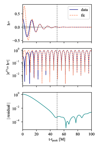
Figure 1: Ringdown time series. The top panel shows the 22 mode numerical-relativity data $h_{+}(t)$, which is the real part of the 22 mode strain, in solid blue alongside a fit obtained using just the 220 and 320 tones predicted by perturbation theory. The dashed vertical line represents the start time for this fit (50M). The grey band represents the artificial noise $\sigma_{\text{sys}}$. The second panel shows the same timeseries, but multiplied by $e^{t/\tau_{220}}$ in order to counteract the exponential decay of the 220 tone. The horizontal line represents our model for the uncertainty $\sigma_{\text{sys}}$ in this regime, which in this representation is constant. The bottom panel shows the difference between the numerical-relativity waveform and our fit as a function of time.

In order to quantify this systematic uncertainty, we fit the late waveform (starting from $t=100M$), allowing for a mixture of the 220, 320 and 221 tones. We choose 100M as the earliest time when the 221 is beginning to become unresolved for an analytic waveform test consisting of three tones with the same frequency and damping times of the 220, 320 and 221 in the numerical-relativity simulation and amplitudes and phases consistent with our fits to the numerical-relativity data.

Ideally one would wait longer than 100M. However, the numerical-relativity error starts to increase from 100M, suggesting the numerical relativity error starts to become more relevant from this point. We model the systematic uncertainty so that the artificial noise on the strain is drawn from a Gaussian distribution with width $\sigma_{\text{sys}}$. The artificial noise is implemented by dividing the data by the exponential term of the 220 tone, $e^{-t/\tau_{220}}$, before performing our fits. $\tau_{220}$ is the damping time of the 220 tone $\approx 11.74M$, calculated using the simulation remnant mass and spin in the qnm package [76].

We vary $\sigma_{\text{sys}}$ until the posterior for the amplitude of the 221 tone $A_{221}$ is consistent with zero at one-sigma credibility. This enforces our requirement that the late-time ringdown should not contain any contribution from overtones higher than the 220. We obtain a value of $\sigma_{\text{sys}}=0.06$, which is $\approx 70$ times higher than the expected numerical-relativity error at $t=100M$. This suggests that our ability to understand the late-time behaviour of the ringdown is likely limited not by numerical-relativity noise, but by theoretical uncertainty about the relative contribution of various tones and/or non-linearities. The quantity $\sigma_{\text{sys}}$ has no physical meaning; it is a purely phenomenological tool that we introduce in order to quantify our present theoretical uncertainty about the behavior of the late-time ringdown.

Our decision to model $\sigma_{\text{sys}}$ with an artificial uncertainty (rather than an absolute uncertainty) is motivated by experimentation. We find that our fits are relatively consistent in size and magnitude and that our sampling is better behaved when we assume an artificial uncertainty as a function of time, while they become difficult to compare assuming a fixed absolute uncertainty. Our model for $\sigma_{\text{sys}}$ is shown in Fig. 1. The top panel shows the real part of the 22 mode numerical-relativity waveform $h_{+}(t)$ and fit. We include a grey band representing our choice for the artificial noise, while the middle panel shows $h_{+}(t)$ multiplied by $e^{t/\tau_{220}}$; the artificial noise $\sigma_{\text{sys}}$ can be visualised as a horizontal line at 0.06 on this panel. The bottom panel is a time series showing the difference between the numerical-relativity waveform and our fit. We provide more details on this approach in Appendix A.

III Results

III.1 Consistency of tones with time

We seek to determine how many and which tones are required to produce a self-consistent measurement of the ringdown signal across time. To this end, it is useful to introduce a criterion to determine if each tone is stably recovered. For a tone to be recovered stably at time $t_{0}$, we require that the 95% credible intervals for the amplitude and phase of that tone overlap with the 95% credible intervals of all subsequent fits (corresponding to larger values of $t_{0}$). Thus, e.g., the fit at $10M$ must be consistent with all the fits between $10M$ and $70M$ to be considered stable at $10M$. We are interested in tones that are both consistent and resolved. In order for a tone to be considered stable and resolved at time $t_{0}$, we further require that the 95% credible interval for the amplitude excludes zero. This creates three possible classifications:

1. Stable recovery. The amplitude of the tone is non-zero and the amplitude and phase of the tone are consistent with subsequent fits.

2. Unstable recovery. The amplitude of the tone is non-zero, but the amplitude and/or phase are inconsistent with subsequent fits.

3. Unresolved. The amplitude of the tone is consistent with zero.

This classification method is illustrated in Fig. 2. Each panel shows amplitude of a different tone as a function of start time $t_{0}$. There are five tones in our fit: 220, 320, 221, 222 and 223. This amounts to four tones of the $\ell=m=2$ QNM plus a contribution from the 320 due to mode-mixing. At regularly spaced values of $t_{0}$, we plot the posterior for each amplitude in teal. The amplitudes are all measured at a reference time of $t=t_{\text{peak}}$ while the fit is performed at different start times $t_{0}$. The background is shaded according to the stability of the tone. The light-gray regions indicate that the tone is unstably recovered, the white regions indicate it is stably recovered, and the dark-gray regions indicate that the tone is unresolved. To avoid clutter, we do not show the accompanying plots of phase, although we also require phase consistency in order for a tone to be classified as stable. We provide the corresponding plot of the phase posteriors in Appendix B.

From the first two panels, we see that the 220 and 320 tones are stably recovered from $t_{0}=0M$. In Appendix C we compare the 220 posteriors for the lowest and highest $n$ fits, demonstrating how the 220 stabilises with the inclusion of more tones. The 221 tone is initially unstably recovered, stabilises at $10M$, and then becomes unresolved at $30M$. The 222 tone is stably recovered within a narrow window around $5-15M$ while the $223$ tone is unresolved. With our framework, the $\ell=m=2$ ringdown signal is well described by four tones which are stable from approximately $10M$, when considering a model allowing 220, 320, 221, 222 and 223 contributions.

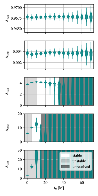
Figure 2: Posterior distributions for amplitude as a function of $t_{0}$. Each panel represents a different tone. We show the regimes where each fit is stably recovered (white), unstably recovered (light gray) and unresolved (dark gray). We also fit the phase of each tone and require the phase to also be stable for that tone to be considered stable. For simplicity we only show the amplitude posteriors here.We show the corresponding phase posteriors in Fig. 6. The 221, 222 and 223 tones are unstably recovered at early times and become unresolved at late times, which implies that they do not significantly improve the fit at late times. The 223 tone is not stably recovered at any time but may stabilise with additional tones.

We investigate how the stability changes with the number of tones. First we investigate the 220 alone. We find that the 220 is not stably recovered until approximately $30M$ unless other tones are included in the fit. This is consistent with the expectation that the 220 should become dominant at late times. Adding the 320 does not improve the stability of the recovery significantly. When we add the 221, the 220 becomes stably recovered at $15M$. The earliest stable time for the 220 changes to $5M$ when we add the 222 and $0M$ when we add the 223.

This analysis suggests that the 22 mode ringdown signal is well described by four tones. Adding the 224 tone may slightly improve the recovery stability of the 222, but does not improve that of the 223 and decays too quickly to be stably recovered itself. The 221 behaviour remains unchanged with the inclusion of the 224. Additional tones produce fits consistent with zero amplitude. Table 1 summarises the recovery stability of different tones as we vary the number of tones $N$.

We test the impact of reducing the spacing in start times $t_{0}$ on our results. We test the five-tone fit using a spacing of $2M$ between $0$ and $20M$ and find the tones behave consistently with the more coarsely spaced test. However, the 221 recovery is slightly improved, stabilising at $6M$, rather than $10M$. The 222 recovery stabilises at $8M$— slightly later than the previous test— and becomes unresolved at $14M$. The 223 recovery remains unstable at all times and becomes unresolved at $12M$.

Table 1: Summary of when each tone is stably recovered for different values of $N_{\text{tones}}$. The variable $t_{\text{stable}}$ indicates the time at which the amplitude and phase of each tone become consistent with subsequent fits using later parts of the waveform (and which the amplitude of the tone is inconsistent with zero). If the tone is not stably recovered for any time, this cell is marked “$-$”. The variable $t_{\text{unresolved}}$ indicates the time at which the amplitude becomes consistent with zero. If the tone is never consistent with zero, this cell is marked “$-$”. $\tau$ denotes the damping time for each tone.

N${}_{\text{tones}}$	tone	$\tau$ [M]	t${}_{\text{stable}}[M]$	t${}_{\text{unresolved}}[M]$
1	220	11.74	30	$-$
2	220	11.74	30	$-$
	320	11.27	0	$-$
3	220	11.74	15	$-$
	320	11.27	5	$-$
	221	3.88	30	45
4	220	11.74	5	$-$
	320	11.27	0	$-$
	221	3.88	20	40
	222	2.30	$-$	20
5	220	11.74	0	$-$
	320	11.27	0	$-$
	221	3.88	10	35
	222	2.30	5	15
	223	1.62	$-$	15

As a consistency check, we assess the goodness-of-fit for each of our models by comparing the maximum log likelihood of each model as a function of time. Figure 3 shows the log likelihood of each model as a function of start time $t_{0}$. The likelihood increases as the number of tones is increased, suggesting that the addition of tones serves to improve the fit, although the improvements are minimal from $30-40M$ after the strain peak.

Figure 3: Maximum natural log likelihood as a function of $t_{0}$ for different values of $N_{\text{tones}}$. (To handle the large dynamic range of likelihood values, we actually plot the $\text{log}_{10}$ of $-\ln{\cal L}_{\text{max}}$.) All four models include the 320 tone. At early times the fits improve as we add tones to the model before saturating at around $30M$, lending further support to to the conclusion that the fit is dominated by the 220 past $30M$.

III.2 How many tones can be resolved at the waveform peak?

Ref. [30] suggests that the perturbative regime can be applied as early as the waveform peak ($t_{0}=0M$), and that seven tones produce the best fit at this time. We investigate the number of tones that can be resolved at $0M$, when the strain amplitude is maximal. We fit our numerical-relativity data with seven tones consisting of the first six (over)tones of the 22 mode and the 320 tone. We find that overtones higher than 224 are not resolved because their amplitude posteriors are consistent with zero. This appears to be consistent with Fig. 9 in [30].

We also test with six tones and find that when the 225 is the highest tone, the 225 can be resolved away from zero, but is not resolved with the addition of the 226. It becomes consistent with zero at the next time step. This suggests that at least some over-fitting is likely occurring for $n=7$ within the framework of our phenomenological noise model, since those higher overtones are not resolved for this fit. Figure 4 shows the posteriors for the amplitudes of each tone included in this fit.

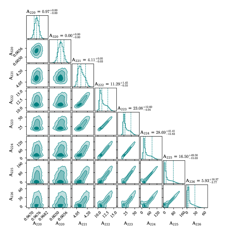
Figure 4: The amplitude posteriors for a seven-tone fit at the strain peak ($t_{0}=0M$). Tones up to $n=4$ are measured confidently with amplitudes consistent with [30], higher overtones return posteriors that support zero. This suggests that including tones higher than the 224 may be over-fitting. We notice that the correlation between tones increases as $n$ increases. This is consistent with the findings of [18], and reflects the increasing difficulty to distinguish between higher tones that decay quickly and may not be stably recovered.

IV Discussion and Conclusions

In this work we introduce a framework to determine under what circumstances a perturbative description can be self-consistently applied to a binary black hole ringdown obtained from numerical relativity simulations. We start near the end of the waveform where the 220 tone is expected to be dominant and work backward, using the late-time waveform to set the scale of systematic uncertainty in our model. We propose a criterion for stability to ensure that the fits obtained at different start times are consistent. We find that it is possible to achieve a self-consistent perturbative description within our framework from $\approx 10M$ after peak strain. The perturbative description does not appear to be stable back to the peak strain.

The 220 is not stably recovered without the addition of the 221 until late times. However, the 221 is only stably recovered and resolvable with this method for a short time interval between $10-35M$. Including the 222 appears to improve the fits at early times and allows the 220 and 221 to be recovered stably at earlier times. The 222 recovery can be briefly stabilised with the addition of the 223. However the 223 is not stably recovered at any of the times we investigate and does not seem to stabilise with the addition of the 224.

The 320 tone, which we add as the dominant contribution from mode mixing, is always stable from the waveform peak. Ref. [30] suggests that the perturbative model can be applied at or before $t_{0}=t_{\text{peak}}$. We show that at $t_{0}=t_{\text{peak}}=0M$ the numerical-relativity data can be explained with no more than five tones (four tones of the 22 mode along with the 320 tone). Any higher tones included in the fit are consistent with zero amplitude.

We have shown that a superposition of quasinormal tones can be used to produce a self-consistent description of the ringdown. However, this does not prove that these fits are “physical” (as opposed to phenomenological) or that the signal is consistent with a perturbed black hole. This study brings into focus a great challenge at the heart of the black-hole spectroscopy program: it is unclear how one can even answer the question of whether the perturbative description is physical or phenomenological. The stability of the quasinormal tone fits is a requirement for their physical interpretability, but further work is required to understand the relation of these observables to the underlying nature of the spacetime and our ability to probe it.

Addendum

As we were preparing this manuscript, we became aware of work by [79] and [80]. Ref. [79] also attempts to extract tones in a self-consistent framework—by iteratively subtracting away the tone with the longest damping time. They find that this technique improves the stability of the extracted amplitude and phases for up to five tones of SXS:0305. This is broadly consistent with our result that only a limited number of tones can be fitted in a self-consistent framework, although we find this is limited to four tones rather than five. They also include the 320 contribution from mode-mixing and find that this improves the stability of the early tones but introduces more instability of tones higher than $n=2$. Ref. [80] uses Bayesian inference to compare the performance of non-linear inspiral-merger-ringdown (IMR) models with linear QNM ringdown models. They find that IMR models produce better fits with higher Bayes factors at early times. They find that overtones may be measurable in high SNR events consistent with third-generation observatories. They caution that the instability of tones may make linear QNM models less reliable than non-linear models for performing tests of general relativity.

Appendix A Noise Model

In the body of this manuscript, we employ an “artificial noise” model in which the systematic uncertainty is a constant error relative to the 220 tone; see Section II. We also test a “flat noise” model in which the systematic uncertainty is constant at all times. In Fig. 5 we show how the flat-noise fits compare to the artificial-noise fits. (For this analysis, we include the 220 and 320 tones.) We find that the posteriors are more comparable in magnitude and size over time using the artificial noise approach. We also find better sampler convergence, which is likely due to the SNR being comparable at early and late times rather than orders of magnitude different. Thus, in order to facilitate a self-consistent overtone model, we employ the artificial noise model in the main body of the manuscript. However we emphasise that this noise model is entirely phenomenological and not physically motivated.

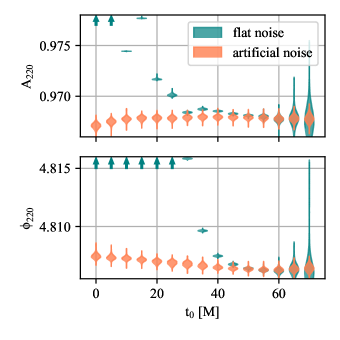
Figure 5: Posterior for amplitude and phase as a function of start time $t_{0}$ for the 220 tone. (The fits also include the 320 tone; not shown here.) The “flat-noise” model (teal) assumes the systematic error does not change with respect to $t_{0}$. The “artificial-noise” model (orange) assumes that systematic error is a constant fraction of the 220 amplitude. The artificial-noise model produces more consistent fits than the flat-noise model.

Appendix B Phase posteriors

In Fig. 6 we plot the phase posteriors of the five-tone fit we present in the main body of the manuscript. The corresponding posteriors for the tone amplitudes are presented in Fig. 2.

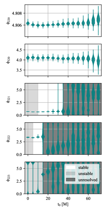
Figure 6: Posterior distributions for phase as a function of $t_{0}$. Each panel represents a different tone. We show the regimes where each fit is stably recovered (white), unstably recovered (light gray) and unresolved (dark gray). The 221, 222 and 223 tones are unstably recovered at early times and become unresolved at late times, which implies that they do not significantly improve the fit at late times. The 223 tone is not stably recovered at any time but may stabilise with additional tones. We show the corresponding amplitude posteriors in Fig. 2.

Appendix C 220 stability

Figure  7 shows the posterior distributions recovered for the 220 tone with the lowest and highest dimensional models included in the study. We also show the median values that are common to all posteriors in the 5-tone fit.

Figure 7: The amplitude and phase posteriors of the 220 tone when measured with a 1 and 5-tone model. The 5-tone model is stable at all times, while the 1-tone model becomes stable at 30M. The dashed horizontal lines show the median of the overlap at 95% confidence for the 5-tone model.

Appendix D Varying the frequency of overtones

In the main body of this manuscript, we assume that the frequency and damping time of each tone are fixed to the values expected from black-hole perturbation theory. Here, we relax this assumption so that the frequency can be treated as a free parameter. We test a three-tone fit including the 220, 320 and 221 tones and allowing the frequency of the 221 to vary. We use a uniform prior between 0.5 and 0.6 for the 221 frequency. Figure 8 shows the result of this fit. The predicted frequency value is shown as a red line in the bottom panel. The predicted frequency is consistent with the posterior only for start times $t_{0}>15M$. The posteriors for other parameters do not change significantly when $f_{221}$ is treated as a free parameter. The fact that the numerical-relativity data prefer the wrong value of $f_{221}$ before $15M$ could mean that non-linearities are present in the data at early times that are influencing the fit. Alternatively, it may be that more tones are required at early times to avoid this behavior, which is what [e.g., 30] would imply.

We also measure the frequency of the 220 tone in a two-mode fit with the 220 and 320 tones. We find that the posterior moves away from the predicted frequency value while the phase becomes unstable. The frequency predicted by general relativity is only recovered for three time steps between 35 and $45M$. In the three- and four-tone models, varying the 221 frequency slightly improves the stability of the first three tones. The general relativity frequency for the 221 is recovered at relatively late times: $15M$ for a three-mode fit and $10M$ for a four-mode fit. This further highlights that caution is required when fitting the tone frequencies due to the uncertain number of tones required, potential non-linearities and non-optimal fits, especially when doing so to test the no-hair theorem as shown in [e.g., 30, 16].

Table 2 summarises the stability of the recovery of each of the tones when we sample the frequency as well as the amplitude and phase. Treating $f_{221}$ as a free parameter helps stabilise the fits at earlier times than when we sample in the amplitude and phase alone. The 221 also remains distinct from zero for an extra time step. However, we see the opposite effect when we treat $f_{220}$ as a free parameter for the two-tone fit. The 220 parameters do not become stable until $60M$ and the 320 tone is slightly affected, stabilising at $5M$ instead of $0M$.

Table 2: The stability of our tones when we vary either the $f_{220}$ or $f_{221}$ as free parameters. In the two-tone fit, we allow $f_{220}$ to vary. In the three- and four-tone fits, we allow $f_{221}$ to vary.

N${}_{\text{tones}}$	tone	$\tau$ [M]	t${}_{\text{stable}}[M]$	t${}_{\text{unresolved}}[M]$
2	220	11.74	60	-
	320	11.27	5	-
3	220	11.74	10	-
	320	11.27	0	-
	221	3.88	20	45
4	220	11.74	5	-
	320	11.27	0	-
	221	3.88	15	35
	222	2.30	-	20

Figure 8: Violin plots showing the posterior distributions for a three-tone fit where $f_{221}$ is treated like a free parameter. Including the 221 makes the 220 fit stable at earlier times. The fit becomes stable at $20M$, which is $10M$ earlier than when we keep $f_{221}$ fixed. Similarly, the 220 becomes stably recovered $5M$ earlier than when $f_{221}$ was fixed.

References

- Vishveshwara [1970] C. V. Vishveshwara, Stability of the schwarzschild metric, Phys. Rev. D 1, 2870 (1970).
- Teukolsky [1973] S. A. Teukolsky, Perturbations of a Rotating Black Hole. I. Fundamental Equations for Gravitational, Electromagnetic, and Neutrino-Field Perturbations, ApJ 185, 635 (1973).
- Chandrasekhar and Detweiler [1975] S. Chandrasekhar and S. Detweiler, The Quasi-Normal Modes of the Schwarzschild Black Hole, Proceedings of the Royal Society of London Series A 344, 441 (1975).
- Leaver [1985] E. W. Leaver, An Analytic representation for the quasi normal modes of Kerr black holes, Proc. Roy. Soc. Lond. A 402, 285 (1985).
- Kokkotas and Schmidt [1999] K. D. Kokkotas and B. G. Schmidt, Quasi-normal modes of stars and black holes, Living Reviews in Relativity 2, 10.12942/lrr-1999-2 (1999).
- Carter [1971] B. Carter, Axisymmetric Black Hole Has Only Two Degrees of Freedom, Phys. Rev. Lett. 26, 331 (1971).
- Dreyer et al. [2004] O. Dreyer, B. J. Kelly, B. Krishnan, L. S. Finn, D. Garrison, and R. Lopez-Aleman, Black hole spectroscopy: Testing general relativity through gravitational wave observations, Class. Quant. Grav. 21, 787 (2004), arXiv:gr-qc/0309007 .
- Berti et al. [2006] E. Berti, V. Cardoso, and C. M. Will, Gravitational-wave spectroscopy of massive black holes with the space interferometer LISA, Physical Review D 73, 10.1103/physrevd.73.064030 (2006).
- Isi et al. [2019] M. Isi, M. Giesler, W. M. Farr, M. A. Scheel, and S. A. Teukolsky, Testing the no-hair theorem with GW150914, Physical Review Letters 123, 10.1103/physrevlett.123.111102 (2019).
- Abbott et al. [2021a] R. Abbott et al. (LIGO Scientific, Virgo), Tests of general relativity with binary black holes from the second LIGO-Virgo gravitational-wave transient catalog, Phys. Rev. D 103, 122002 (2021a), arXiv:2010.14529 [gr-qc] .
- Cotesta et al. [2022] R. Cotesta, G. Carullo, E. Berti, and V. Cardoso, Analysis of ringdown overtones in GW150914, Physical Review Letters 129, 10.1103/physrevlett.129.111102 (2022).
- Abbott et al. [2021b] R. Abbott et al. (LIGO Scientific, VIRGO, KAGRA), Tests of General Relativity with GWTC-3, arXiv e-prints (2021b), arXiv:2112.06861 [gr-qc] .
- Nollert [1996] H.-P. Nollert, About the significance of quasinormal modes of black holes, Phys. Rev. D 53, 4397 (1996), arXiv:gr-qc/9602032 [gr-qc] .
- Thrane et al. [2017] E. Thrane, P. D. Lasky, and Y. Levin, Challenges for testing the no-hair theorem with current and planned gravitational-wave detectors, Phys. Rev. D 96, 102004 (2017), arXiv:1706.05152 [gr-qc] .
- Bhagwat et al. [2018] S. Bhagwat, M. Okounkova, S. W. Ballmer, D. A. Brown, M. Giesler, M. A. Scheel, and S. A. Teukolsky, On choosing the start time of binary black hole ringdowns, Phys. Rev. D 97, 104065 (2018), arXiv:1711.00926 [gr-qc] .
- Isi and Farr [2021] M. Isi and W. M. Farr, Analyzing black-hole ringdowns, arXiv e-prints , arXiv:2107.05609 (2021), arXiv:2107.05609 [gr-qc] .
- Abbott et al. [2016a] B. P. Abbott et al., Tests of General Relativity with GW150914, Phys. Rev. Lett. 116, 221101 (2016a), arXiv:1602.03841 [gr-qc] .
- Bhagwat et al. [2020] S. Bhagwat, X. J. Forteza, P. Pani, and V. Ferrari, Ringdown overtones, black hole spectroscopy, and no-hair theorem tests, Phys. Rev. D 101, 044033 (2020), arXiv:1910.08708 [gr-qc] .
- Baibhav et al. [2023] V. Baibhav, M. H.-Y. Cheung, E. Berti, V. Cardoso, G. Carullo, R. Cotesta, W. Del Pozzo, and F. Duque, Agnostic black hole spectroscopy: Quasinormal mode content of numerical relativity waveforms and limits of validity of linear perturbation theory, Phys. Rev. D 108, 104020 (2023), arXiv:2302.03050 [gr-qc] .
- Bustillo et al. [2021] J. C. Bustillo, P. D. Lasky, and E. Thrane, Black-hole spectroscopy, the no-hair theorem, and GW150914: Kerr versus Occam, Phys. Rev. D 103, 024041 (2021).
- Pretorius [2005] F. Pretorius, Numerical relativity using a generalized harmonic decomposition, Classical and Quantum Gravity 22, 425 (2005), arXiv:gr-qc/0407110 [gr-qc] .
- Campanelli et al. [2006] M. Campanelli, C. O. Lousto, P. Marronetti, and Y. Zlochower, Accurate Evolutions of Orbiting Black-Hole Binaries without Excision, Phys. Rev. Lett. 96, 111101 (2006), arXiv:gr-qc/0511048 [gr-qc] .
- Baker et al. [2006] J. G. Baker, J. Centrella, D.-I. Choi, M. Koppitz, and J. van Meter, Gravitational-wave extraction from an inspiraling configuration of merging black holes, Physical Review Letters 96, 10.1103/physrevlett.96.111102 (2006).
- Buonanno et al. [2007] A. Buonanno, G. B. Cook, and F. Pretorius, Inspiral, merger, and ring-down of equal-mass black-hole binaries, Phys. Rev. D 75, 124018 (2007), arXiv:gr-qc/0610122 [gr-qc] .
- Baibhav et al. [2018] V. Baibhav, E. Berti, V. Cardoso, and G. Khanna, Black hole spectroscopy: Systematic errors and ringdown energy estimates, Phys. Rev. D 97, 044048 (2018), arXiv:1710.02156 [gr-qc] .
- Ota and Chirenti [2020] I. Ota and C. Chirenti, Overtones or higher harmonics? Prospects for testing the no-hair theorem with gravitational wave detections, Phys. Rev. D 101, 104005 (2020), arXiv:1911.00440 [gr-qc] .
- Mourier et al. [2021] P. Mourier, X. Jiménez Forteza, D. Pook-Kolb, B. Krishnan, and E. Schnetter, Quasinormal modes and their overtones at the common horizon in a binary black hole merger, Phys. Rev. D 103, 044054 (2021), arXiv:2010.15186 [gr-qc] .
- Sago et al. [2021] N. Sago, S. Isoyama, and H. Nakano, Fundamental Tone and Overtones of Quasinormal Modes in Ringdown Gravitational Waves: A Detailed Study in Black Hole Perturbation, Universe 7, 357 (2021), arXiv:2108.13017 [gr-qc] .
- Li et al. [2022] X. Li, L. Sun, R. K. L. Lo, E. Payne, and Y. Chen, Angular emission patterns of remnant black holes, Phys. Rev. D 105, 024016 (2022), arXiv:2110.03116 [gr-qc] .
- Giesler et al. [2019] M. Giesler, M. Isi, M. A. Scheel, and S. A. Teukolsky, Black Hole Ringdown: The Importance of Overtones, Physical Review X 9, 041060 (2019), arXiv:1903.08284 [gr-qc] .
- Ma et al. [2022] S. Ma, K. Mitman, L. Sun, N. Deppe, F. Hébert, L. E. Kidder, J. Moxon, W. Throwe, N. L. Vu, and Y. Chen, Quasinormal-mode filters: A new approach to analyze the gravitational-wave ringdown of binary black-hole mergers, Phys. Rev. D 106, 084036 (2022), arXiv:2207.10870 [gr-qc] .
- Cook [2020] G. B. Cook, Aspects of multimode Kerr ringdown fitting, Phys. Rev. D 102, 024027 (2020), arXiv:2004.08347 [gr-qc] .
- Zertuche et al. [2022] L. M. Zertuche, K. Mitman, N. Khera, L. C. Stein, M. Boyle, N. Deppe, F. Hébert, D. A. B. Iozzo, L. E. Kidder, J. Moxon, H. P. Pfeiffer, M. A. Scheel, S. A. Teukolsky, W. Throwe, and N. Vu, High precision ringdown modeling: Multimode fits and BMS frames, Phys. Rev. D 105, 104015 (2022).
- Forteza and Mourier [2021] X. J. Forteza and P. Mourier, High-overtone fits to numerical relativity ringdowns: Beyond the dismissed n =8 special tone, Phys. Rev. D 104, 124072 (2021), arXiv:2107.11829 [gr-qc] .
- Okounkova [2020] M. Okounkova, Revisiting non-linearity in binary black hole mergers, arXiv e-prints , arXiv:2004.00671 (2020), arXiv:2004.00671 [gr-qc] .
- Chen et al. [2022] Y. Chen, P. Kumar, N. Khera, N. Deppe, A. Dhani, M. Boyle, M. Giesler, L. E. Kidder, H. P. Pfeiffer, M. A. Scheel, and S. A. Teukolsky, Multipole moments on the common horizon in a binary-black-hole simulation, Physical Review D 106, 10.1103/physrevd.106.124045 (2022).
- Mitman et al. [2023] K. Mitman, M. Lagos, L. C. Stein, S. Ma, L. Hui, Y. Chen, N. Deppe, F. Hébert, L. E. Kidder, J. Moxon, M. A. Scheel, S. A. Teukolsky, W. Throwe, and N. L. Vu, Nonlinearities in Black Hole Ringdowns, Phys. Rev. Lett. 130, 081402 (2023), arXiv:2208.07380 [gr-qc] .
- Cheung et al. [2023] M. H.-Y. Cheung, V. Baibhav, E. Berti, V. Cardoso, G. Carullo, R. Cotesta, W. Del Pozzo, F. Duque, T. Helfer, E. Shukla, and K. W. Wong, Nonlinear effects in black hole ringdown, Physical Review Letters 130, 10.1103/physrevlett.130.081401 (2023).
- Pook-Kolb et al. [2020] D. Pook-Kolb, O. Birnholtz, J. L. Jaramillo, B. Krishnan, and E. Schnetter, Horizons in a binary black hole merger II: Fluxes, multipole moments and stability, arXiv e-prints , arXiv:2006.03940 (2020), arXiv:2006.03940 [gr-qc] .
- London et al. [2014] L. London, D. Shoemaker, and J. Healy, Modeling ringdown: Beyond the fundamental quasinormal modes, Phys. Rev. D 90, 124032 (2014), arXiv:1404.3197 [gr-qc] .
- London [2020] L. London, Modeling ringdown. ii. aligned-spin binary black holes, implications for data analysis and fundamental theory, Physical Review D 102, 10.1103/physrevd.102.084052 (2020).
- Jiménez Forteza et al. [2020] X. Jiménez Forteza, S. Bhagwat, P. Pani, and V. Ferrari, Spectroscopy of binary black hole ringdown using overtones and angular modes, Phys. Rev. D 102, 044053 (2020), arXiv:2005.03260 [gr-qc] .
- Zhu et al. [2023] H. Zhu, J. L. Ripley, A. Cárdenas-Avendaño, and F. Pretorius, Challenges in Quasinormal Mode Extraction: Perspectives from Numerical solutions to the Teukolsky Equation, arXiv e-prints , arXiv:2309.13204 (2023), arXiv:2309.13204 [gr-qc] .
- Nee et al. [2023] P. J. Nee, S. H. Völkel, and H. P. Pfeiffer, Role of black hole quasinormal mode overtones for ringdown analysis, Phys. Rev. D 108, 044032 (2023), arXiv:2302.06634 [gr-qc] .
- Ho-Yeuk Cheung et al. [2023] M. Ho-Yeuk Cheung, E. Berti, V. Baibhav, and R. Cotesta, Extracting linear and nonlinear quasinormal modes from black hole merger simulations, arXiv e-prints , arXiv:2310.04489 (2023), arXiv:2310.04489 [gr-qc] .
- Carullo et al. [2019] G. Carullo, W. D. Pozzo, and J. Veitch, Observational black hole spectroscopy: A time-domain multimode analysis of GW150914, Physical Review D 99, 10.1103/physrevd.99.123029 (2019).
- Wang et al. [2023] Y.-F. Wang, C. D. Capano, J. Abedi, S. Kastha, B. Krishnan, A. B. Nielsen, A. H. Nitz, and J. Westerweck, A frequency-domain perspective on GW150914 ringdown overtone, arXiv e-prints , arXiv:2310.19645 (2023), arXiv:2310.19645 [gr-qc] .
- Ma et al. [2023] S. Ma, L. Sun, and Y. Chen, Using rational filters to uncover the first ringdown overtone in GW150914, Phys. Rev. D 107, 084010 (2023), arXiv:2301.06639 [gr-qc] .
- Finch and Moore [2022] E. Finch and C. J. Moore, Searching for a ringdown overtone in GW150914, Phys. Rev. D 106, 043005 (2022), arXiv:2205.07809 [gr-qc] .
- Wang and Shao [2023] H.-T. Wang and L. Shao, Effect of Noise Estimation in Time-Domain Ringdown Analysis: A Case Study with GW150914, arXiv e-prints , arXiv:2311.13300 (2023), arXiv:2311.13300 [gr-qc] .
- Crisostomi et al. [2023] M. Crisostomi, K. Dey, E. Barausse, and R. Trotta, Neural posterior estimation with guaranteed exact coverage: The ringdown of GW150914, Phys. Rev. D 108, 044029 (2023), arXiv:2305.18528 [gr-qc] .
- Correia et al. [2023] A. Correia, Y.-F. Wang, and C. D. Capano, Low evidence for ringdown overtone in GW150914 when marginalizing over time and sky location uncertainty, arXiv e-prints , arXiv:2312.14118 (2023), arXiv:2312.14118 [gr-qc] .
- Isi and Farr [2023] M. Isi and W. M. Farr, Comment on “Analysis of Ringdown Overtones in GW150914”, Phys. Rev. Lett. 131, 169001 (2023), arXiv:2310.13869 [astro-ph.HE] .
- Carullo et al. [2023] G. Carullo, R. Cotesta, E. Berti, and V. Cardoso, Reply to Comment on ”Analysis of Ringdown Overtones in GW150914”, Phys. Rev. Lett. 131, 169002 (2023), arXiv:2310.20625 [gr-qc] .
- Capano et al. [2021] C. D. Capano, M. Cabero, J. Westerweck, J. Abedi, S. Kastha, A. H. Nitz, Y.-F. Wang, A. B. Nielsen, and B. Krishnan, Observation of a multimode quasi-normal spectrum from a perturbed black hole, arXiv e-prints , arXiv:2105.05238 (2021), arXiv:2105.05238 [gr-qc] .
- Siegel et al. [2023] H. Siegel, M. Isi, and W. M. Farr, Ringdown of GW190521: Hints of multiple quasinormal modes with a precessional interpretation, Phys. Rev. D 108, 064008 (2023), arXiv:2307.11975 [gr-qc] .
- Abbott et al. [2020] R. Abbott, T. D. Abbott, S. Abraham, F. Acernese, K. Ackley, C. Adams, R. X. Adhikari, V. B. Adya, C. Affeldt, M. Agathos, and et al., GW190521: A Binary Black Hole Merger with a Total Mass of 150 M⊙, Phys. Rev. Lett. 125, 101102 (2020), arXiv:2009.01075 [gr-qc] .
- Berti et al. [2009] E. Berti, V. Cardoso, and A. O. Starinets, TOPICAL REVIEW: Quasinormal modes of black holes and black branes, Classical and Quantum Gravity 26, 163001 (2009), arXiv:0905.2975 [gr-qc] .
- Berti [2023] E. Berti, Ringdown (2023), [Online; accessed 30-October-2023].
- Teukolsky [1972] S. A. Teukolsky, Rotating Black Holes: Separable Wave Equations for Gravitational and Electromagnetic Perturbations, Phys. Rev. Lett. 29, 1114 (1972).
- Mroué et al. [2013] A. H. Mroué, M. A. Scheel, B. Szilágyi, H. P. Pfeiffer, M. Boyle, D. A. Hemberger, L. E. Kidder, G. Lovelace, S. Ossokine, N. W. Taylor, A. Zenginoğlu, L. T. Buchman, T. Chu, E. Foley, M. Giesler, R. Owen, and S. A. Teukolsky, Catalog of 174 Binary Black Hole Simulations for Gravitational Wave Astronomy, Phys. Rev. Lett. 111, 241104 (2013), arXiv:1304.6077 [gr-qc] .
- Boyle et al. [2019] M. Boyle, D. Hemberger, D. A. B. Iozzo, G. Lovelace, S. Ossokine, H. P. Pfeiffer, M. A. Scheel, L. C. Stein, C. J. Woodford, A. B. Zimmerman, N. Afshari, K. Barkett, J. Blackman, K. Chatziioannou, T. Chu, N. Demos, N. Deppe, S. E. Field, N. L. Fischer, E. Foley, H. Fong, A. Garcia, M. Giesler, F. Hebert, I. Hinder, R. Katebi, H. Khan, L. E. Kidder, P. Kumar, K. Kuper, H. Lim, M. Okounkova, T. Ramirez, S. Rodriguez, H. R. Rüter, P. Schmidt, B. Szilagyi, S. A. Teukolsky, V. Varma, and M. Walker, The SXS collaboration catalog of binary black hole simulations, Classical and Quantum Gravity 36, 195006 (2019), arXiv:1904.04831 [gr-qc] .
- Mitman et al. [2020] K. Mitman, J. Moxon, M. A. Scheel, S. A. Teukolsky, M. Boyle, N. Deppe, L. E. Kidder, and W. Throwe, Computation of displacement and spin gravitational memory in numerical relativity, Phys. Rev. D 102, 104007 (2020), arXiv:2007.11562 [gr-qc] .
- Moxon et al. [2020] J. Moxon, M. A. Scheel, and S. A. Teukolsky, Improved Cauchy-characteristic evolution system for high-precision numerical relativity waveforms, Phys. Rev. D 102, 044052 (2020), arXiv:2007.01339 [gr-qc] .
- Moxon et al. [2021] J. Moxon, M. A. Scheel, S. A. Teukolsky, N. Deppe, N. Fischer, F. Hébert, L. E. Kidder, and W. Throwe, The SpECTRE Cauchy-characteristic evolution system for rapid, precise waveform extraction, arXiv e-prints , arXiv:2110.08635 (2021), arXiv:2110.08635 [gr-qc] .
- Deppe et al. [2023] N. Deppe, W. Throwe, L. E. Kidder, N. L. Vu, K. C. Nelli, C. Armaza, M. S. Bonilla, F. Hébert, Y. Kim, P. Kumar, G. Lovelace, A. Macedo, J. Moxon, E. O’Shea, H. P. Pfeiffer, M. A. Scheel, S. A. Teukolsky, N. A. Wittek, I. Anantpurkar, C. Anderson, M. Boyle, A. Carpenter, A. Ceja, H. Chaudhary, N. Corso, F. Foucart, N. Ghadiri, M. Giesler, J. S. Guo, D. A. B. Iozzo, K. Z. Jones, G. Lara, I. Legred, D. Li, S. Ma, D. Melchor, M. Morales, E. R. Most, P. J. Nee, A. Osorio, M. A. Pajkos, K. Pannone, T. Ramirez, N. Ring, H. R. Rüter, J. Sanchez, L. C. Stein, D. Tellez, S. Thomas, D. Vieira, T. Wlodarczyk, D. Wu, and J. Yoo, Spectre (2023).
- Mitman et al. [2021] K. Mitman, N. Khera, D. A. B. Iozzo, L. C. Stein, M. Boyle, N. Deppe, L. E. Kidder, J. Moxon, H. P. Pfeiffer, M. A. Scheel, S. A. Teukolsky, and W. Throwe, Fixing the bms frame of numerical relativity waveforms, Physical Review D 104, 10.1103/physrevd.104.024051 (2021).
- Mitman et al. [2022] K. Mitman, L. C. Stein, M. Boyle, N. Deppe, F. Hébert, L. E. Kidder, J. Moxon, M. A. Scheel, S. A. Teukolsky, W. Throwe, and N. L. Vu, Fixing the bms frame of numerical relativity waveforms with bms charges, Physical Review D 106, 10.1103/physrevd.106.084029 (2022).
- Boyle [2013] M. Boyle, Angular velocity of gravitational radiation from precessing binaries and the corotating frame, Physical Review D 87, 10.1103/physrevd.87.104006 (2013).
- Boyle et al. [2014] M. Boyle, L. E. Kidder, S. Ossokine, and H. P. Pfeiffer, Gravitational-wave modes from precessing black-hole binaries, arXiv e-prints , arXiv:1409.4431 (2014), arXiv:1409.4431 [gr-qc] .
- Boyle [2016] M. Boyle, Transformations of asymptotic gravitational-wave data, Physical Review D 93, 10.1103/physrevd.93.084031 (2016).
- Boyle et al. [2023] M. Boyle, D. Iozzo, L. Stein, A. Khairnar, H. Rüter, M. Scheel, V. Varma, and K. Mitman, scri (2023).
- Abbott et al. [2016b] B. P. Abbott et al., Observation of Gravitational Waves from a Binary Black Hole Merger, Phys. Rev. Lett. 116, 061102 (2016b), arXiv:1602.03837 [gr-qc] .
- Foreman-Mackey et al. [2013] D. Foreman-Mackey, D. W. Hogg, D. Lang, and J. Goodman, emcee: The MCMC Hammer, PASP 125, 306 (2013), arXiv:1202.3665 [astro-ph.IM] .
- Sberna et al. [2022] L. Sberna, P. Bosch, W. E. East, S. R. Green, and L. Lehner, Nonlinear effects in the black hole ringdown: Absorption-induced mode excitation, Phys. Rev. D 105, 064046 (2022), arXiv:2112.11168 [gr-qc] .
- Stein [2019] L. C. Stein, qnm: A Python package for calculating Kerr quasinormal modes, separation constants, and spherical-spheroidal mixing coefficients, J. Open Source Softw. 4, 1683 (2019), arXiv:1908.10377 [gr-qc] .
- Leaver [1986] E. W. Leaver, Spectral decomposition of the perturbation response of the schwarzschild geometry, Phys. Rev. D 34, 384 (1986).
- Carullo and De Amicis [2023] G. Carullo and M. De Amicis, Late-time tails in nonlinear evolutions of merging black hole binaries, arXiv e-prints , arXiv:2310.12968 (2023), arXiv:2310.12968 [gr-qc] .
- Takahashi and Motohashi [2023] K. Takahashi and H. Motohashi, Iterative extraction of overtones from black hole ringdown, arXiv e-prints , arXiv:2311.12762 (2023), arXiv:2311.12762 [gr-qc] .
- Qiu et al. [2023] Y. Qiu, X. Jiménez Forteza, and P. Mourier, Linear vs. nonlinear modelling of black hole ringdowns, arXiv e-prints , arXiv:2312.15904 (2023), arXiv:2312.15904 [gr-qc] .