Convolutional restricted Boltzmann machine (CRBM) correlated variational wave function for the Hubbard model on a square lattice: Mott metal-insulator transition

Abstract

We use a convolutional restricted Boltzmann machine (CRBM) neural network to construct a variational wave function (WF) for the Hubbard model on a square lattice and study it using the variational Monte Carlo (VMC) method. In the wave function, the CRBM acts as a correlation factor to a mean-field BCS state. The number of variational parameters in the WF does not grow automatically with the lattice size and it is computationally much more efficient compared to other neural network based WFs. We find that in the intermediate to strong coupling regime of the model at half-filling, the wave function outperforms even the highly accurate long range backflow-Jastrow correlated wave function. Using the WF, we study the ground state of the half-filled model as a function of onsite Coulomb repulsion $U$. We consider two cases for the next-nearest-neighbor hopping parameter, e.g., $t^{\prime}=0$ as well as a frustrated model case with $t^{\prime}\neq 0$. By examining several quantities, e.g., double occupancy, charge gap, momentum distribution, and spin-spin correlations, we find that the weekly correlated phase in both cases is paramagnetic metallic (PM). As $U$ is increased, the system undergoes a first-order Mott transition to an insulating state at a critical $U_{c}$, the value of which depends upon $t^{\prime}$. The Mott state in both cases is spin gapped with long range antiferromagnetic (AF) order. Remarkably, the AF order emerges spontaneously from the wave function which does not have any explicitly broken symmetry in it. Apart from some quantitative differences in the results for the two values of $t^{\prime}$, we find some interesting qualitative differences in the way the Mott transition takes place in the two cases.

I Introduction

The Hubbard Hamiltonian has been studied extensively over the years using a variety of analytical and numerical methods as a paradigmatic model for various correlated electron phenomenaImada et al. (1998); LeBlanc et al. (2015). The model on a two-dimensional lattice is particularly interesting because of its relevance to the high-temperature superconductorsLee et al. (2006a). Theoretically, the model is handled well both in the weak and strong coupling limits by different methods, but not so in the most interesting intermediate coupling regime. Among various numerical methods, the variational Monte Carlo (VMC) technique has been a very useful over the years in the study of the ground state properties of the model and its various extensionsCeperley et al. (1977); Tahara and Imada (2008); Sorella (2013); Paramekanti et al. (2004); SHIBA and YOKOYAMA (1987). Unlike other methods, VMC does not suffer from any particular difficulty at any coupling strength, but its results are always biased by the choice of the variational wave function (WF) which is generally constructed based on the ground state of an underlying mean-field Hamiltonian. However, with the advent of machine learning algorithms based on artificial neural networks (ANNs), it was realized that ANNs can also be used to represent a quantum many-body wave function Carrasquilla and Melko (2017); Carleo and Troyer (2017); van Nieuwenburg et al. (2017); Broecker et al. (2017); Ch’ng et al. (2017); Deng et al. (2017). In such wave functions termed as neural-network quantum states (NQS), the number of variational degrees of freedom is large and it offers the possibility to overcome the fundamental limitation of the variational method by enabling the construction of a highly unbiased variational wave function.

A number of seminal works have already demonstrated the power of NQS to learn quantum many-body physicsCarleo et al. (2019); Ch’ng et al. (2017); Carrasquilla (2020); Melko et al. (2019); Carrasquilla and Torlai (2021). To mention some of these, Carleo and TroyerCarleo and Troyer (2017) first demonstrated the use of a restricted Boltzmann machine (RBM) based variational wave function to represent the ground state and study the dynamics of a few prototypical spin Hamiltonians accurately and efficiently. The method involved training the network by using a reinforcement learning mechanism which essentially is an iterative tuning of the network parameters so as to minimize the variational energy. Torlai et al.Torlai et al. (2018) used an NQS wave function based on RBM network to perform a quantum state tomography and thereby learn the ground state of a quantum spin Hamiltonian. In Ref. Carleo et al., 2018, the authors used a wave function based on deep Boltzmann machine (DBM) and performed imaginary time evolution to obtain accurate ground state of the transverse-field Ising and the Heisenberg model. Choo et al.Choo et al. (2018), by incorporating translational symmetries explicitly into the NQS wave function, managed to generate also the excited states for the Heisenberg and Bose-Hubbard model. RBM were also shown to be very efficient in representing topological quantum states due to the non-local geometry of its architectureLu et al. (2019); Glasser et al. (2018). However, most of these applications so far have been to bosonic systems. One main reason for this is that the fermionic systems have an additional complexity that comes from the non-trivial sign structures of its wave functionsZhang and Weng (2014). The functions that can be represented by neural-networks though highly non-linear, are essentially smooth and generally fail to represent the sign structures of fermionic many-body wave functions. For instance, the feed-forward neural networks, a type of ANN, were shown to be unable to correctly account for the sign structure of even a free fermionic wave functionCai and Liu (2018). Nomura et al.Nomura et al. (2017) constructed a wave function by combining an RBM with a mean-field part where the RBM part introduces correlation effects, a role usually played by Jastrow type correlation factorsSorella (2013). It was shown that the combination wave function give substantially lower energy than the conventional projected variational wave functions for the fermionic Hubbard model as well as the Heisenberg model. There also exist other schemes based ANNs for fermionic systems but these are restricted to small system size due to computational complexityInui et al. (2021); Luo and Clark (2019); Pfau et al. (2020).

In this work, we construct a ground state variational wave function for the fermionic Hubbard model on a square lattice using a convolutional restricted Boltzmann machine (CRBM) network where the CRBM is used as a correlation factor to a mean-field BCS state. We show that the wave function is not only computationally efficient compared to RBM wave function, it is also highly accurate in terms of the variational energy. Using VMC, we study the wave function as a ground state of the model at half-filling as a function of onsite Coulomb repulsion $U$. We consider two cases of the model when the next-nearest-neighbor hopping parameter $t^{\prime}=0$ and when the model is frustrated with $t^{\prime}\neq 0$. The wave function yields energies which are significantly lower compared to those of the corresponding RBM or Jastrow projected wave functions, especially in the strong coupling limit. Indeed, in this limit it outperforms in terms of energy even the highly accurate long range backflow-Jastrow correlated wave function for the model. The wave function correctly captures the presence of doublon-holon (DH) binding in the strong coupling regime in spite of it having no explicit DH binding term. It also give rise to long range antiferromagnetic (AF) order in the Mott insulating state spontaneously even though the wave function contains no explicit magnetic order. We examine the nature of Mott metal-insulator transition in the model by calculating various quantities, such as double occupancy, charge gap, momentum distribution and quasiparticle weight, and spin-spin correlation. The results are thoroughly discussed and compared with other variational results. The rest of the paper is organized as follows. In section II, we describe the model and the CRBM wave function. In section III, we describe and discuss the results, and finally in section IV, we make the concluding remarks.

II Model and method

We consider the fermionic Hubbard model on a two-dimensional (2D) square lattice at half-filling. The Hamiltonian is given by,

$$\mathcal{H}=-\sum_{i,j\sigma}t_{ij}\left(c^{\dagger}_{i\sigma}c_{j\sigma}+hc\right)+U\sum_{i}n_{i\uparrow}n_{i\downarrow}$$ (1)

where the operator $c^{\dagger}_{i\sigma}$ creates an electron at site ‘$i$’ with spin $\sigma$. $c_{i\sigma}$ is the corresponding annihilation operator and $n_{i\sigma}=c^{\dagger}_{i\sigma}c_{i\sigma}$ is the number operator. The first term represents hoppings of electrons from site to site. The hopping integrals are $t_{ij}=t$ for $i$, $j$ nearest-neighbor (NN) sites, $t_{ij}=-t^{\prime}$ for $i$, $j$ next-nearest-neighbor (NNN) sites, and zero otherwise. Due to the particle-hole symmetry at half-filling, the model is equivalent to the case with opposite sign of $t^{\prime}$. The Hamiltonian is the simplest paradigmatic model that capture the essential physics of several interesting correlated electron phenomenon in condensed matter physics, including Mott metal-insulator transition, high-temperature cuprate superconductors, etc.MOTT (1968); Imada et al. (1998); Orenstein and Millis (2000); Lee et al. (2006b). The Mott physics in the Hubbard model has been studied extensively using various methods Georges et al. (1996); Zhang et al. (1993); Rozenberg et al. (1994); Park et al. (2008); Rozenberg et al. (1999); Bulla et al. (2001); Lu (1994); Ferrero et al. (2005); Rüegg et al. (2005); Mukherjee and Lal (2020), including variational theory within the framework of various Gutzwiller-Jastrow type wave functions (WFs)Yokoyama and Shiba (1990); Yokoyama et al. (2006); Capello et al. (2005, 2006); Tocchio et al. (2008, 2011). These projected variational wave functions are typically of the form, $|\Psi_{var}\rangle={\cal P}\ket{\Phi}$, where $\ket{\Phi}$ is a one-body wave function which is generally taken to be ground state of an underlying mean-field Hamiltonian. ${\cal P}$ is a projection operator or correlation factor which introduces many-body correlation into the wave function. The simplest case is the Gutzwiller (GW) projector ${\cal P}_{G}$ which describes an on-site density-density correlation, ${\cal P}_{G}=\prod_{i}\left[1-(1-g)n_{i\uparrow}n_{i\downarrow}\right]$, $0<g\leq 1$. It penalizes electronic configurations with doubly occupied sites thereby giving a better description of the ground state of the Hubbard model compared to the uncorrelated state. However, GW projector was found to be inadequate to describe the Mott insulating state. This is because in the Mott state, local charge fluctuations creates configurations with doubly occupied sites (doublon) next to empty sites (holon). The insulating nature of the state means that the doublons and holons must be bound to each other and the GW projector does not capture this effectKaplan et al. (1982); Yokoyama et al. (2006); Capello et al. (2005, 2006). It was shown that the situation can be greatly improved by considering a correlation factor of the form ${\cal P}={\cal P}_{DH}{\cal P}_{G}$, where the factor ${\cal P}_{DH}$ incorporates doublon-holon (DH) binding in the wave function and is given byYokoyama et al. (2006), ${\cal P}_{DH}=\prod_{i}\left(1-\eta Q_{i}\right)$, with $Q_{i}=\prod_{\delta}\left[d_{i}(1-h_{i+\delta})+h_{i}(1+d_{i+\delta})\right]$. Here $d_{i}=n_{i\uparrow}n_{i\downarrow}$ is doublon and $h_{i}=(1-n_{i\uparrow})(1-n_{i\downarrow})$ is holon operator, $\delta$ denotes the nearest-neighbor sites, and $\eta$ is a variational parameter. Alternatively, one can also consider Jastrow factor of the formCapello et al. (2005), ${\cal P}_{J}=\exp\left(\sum_{ij}\frac{1}{2}v_{ij}(n_{i}-1)(n_{j}-1)+w_{ij}h_{i}d_{j}\right)$ which introduces long range correlations including DH binding. The description can be further improved by introducing a backflow correlation term in addition to the Jastrow factor and such a wave function considered for the half-filled Hubbard model was shown to be much better in terms of the ground state energy and in the description of the Mott insulating state in the modelTocchio et al. (2011).

Here, we consider a variational wave function where the correlator is based on an artificial neural-network (ANN). Such a wave function using the restricted Boltzmann machine (RBM) network as a correlator was already considered for the Hubbard as well as the Heisenberg modelNomura et al. (2017). Here we consider a convolutional restricted Boltzmann machine (CRBM) network as a correlator. The CRBM is computationally much more efficient than an RBM owing to much lesser number of network connections and consequently fewer number of variational parameters in CRBM. In fact, the number of variational parameters in CRBM can be tuned and does not grow automatically with the lattice size which is a much desirable feature computationally. In the followings, first we describe the RBM network followed by a detailed description of the structure of the CRBM network. The variational wave function using the CRBM as a correlator is described next.

II.1 RBM network

A restricted Boltzmann machine (RBM) networkCarleo et al. (2018) consists of two layers of artificial neurons, one visible layer connected to a hidden layer as shown in Fig. 1. There is no intralayer connection between the neurons.

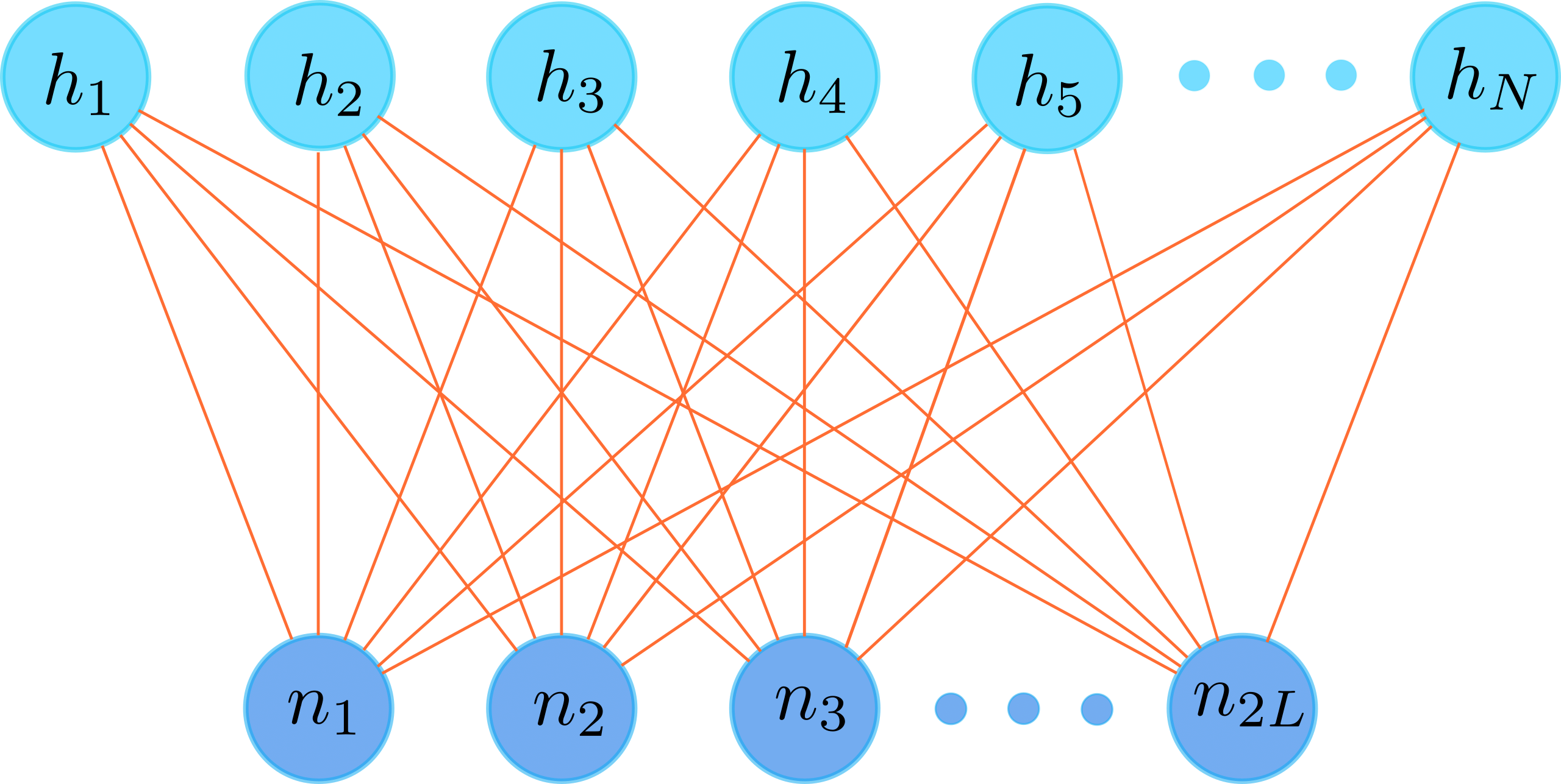
Figure 1: A restricted Boltzmann machine (RBM) network. The artificial neurons in the visible layer take the inputs $\{n_{1},n_{2},\ldots,n_{2L}\}$ that represent the sets of electron occupation numbers. The neurons in the hidden layer define variables $h_{i}$ which can take values $\pm 1$.

The number of neurons in the visible layer is $N_{v}=2L$ where $L$ is the number of lattice sites and that in the hidden layer is $N_{h}$. The energy function of an RBM is given by,

$$E_{RBM}=-\sum_{i,j}w_{ij}h_{i}n_{j}-\sum_{j}a_{j}n_{j}-\sum_{i}b_{i}h_{i}$$ (2)

The hidden variables $h_{i}$ take values $h_{i}=\pm 1$. The set $W=\{\bf a,b,w\}$ denotes the set of all the network parameters $a_{i}$, $b_{j}$, and $w_{ij}$. Carrying out the summation over the hidden variables, the probability distribution over the set of input values $\{n_{1},n_{2},\ldots n_{2L}\}$ is given by,

$$\Psi_{RBM}(R,W)=\frac{1}{Z}\sum_{\bf h}e^{-E_{RBM}}$$ (3)

where $Z$ is the partition function. The number of parameters in the network can be drastically reduced by using the symmetries of the Hamiltonian. Here we take the hidden variable density to be $\alpha=N_{h}/N_{v}=1$. In this case, it can easily be seen that imposition of lattice translational symmetry leads to a single bias parameter $a$ for the visible units and a parameter $b$ for the hidden units. Also the number of unique elements in the weight matrix $w$ reduces to $2L$. Thus the total number of network parameters becomes $(2L+2)$ and the probability function reduces to,

$$\Psi_{RBM}(R,{W})=\frac{1}{Z}e^{a\sum_{i}n_{i}}\prod_{i}2\cosh\Bigl(\sum_{j}w_{ij}n_{j}+b\Bigr{missing})$$ (4)

II.2 CRBM network

The convolutional restricted Boltzmann machine (CRBM) architecture is shown schematically in Fig. 2.

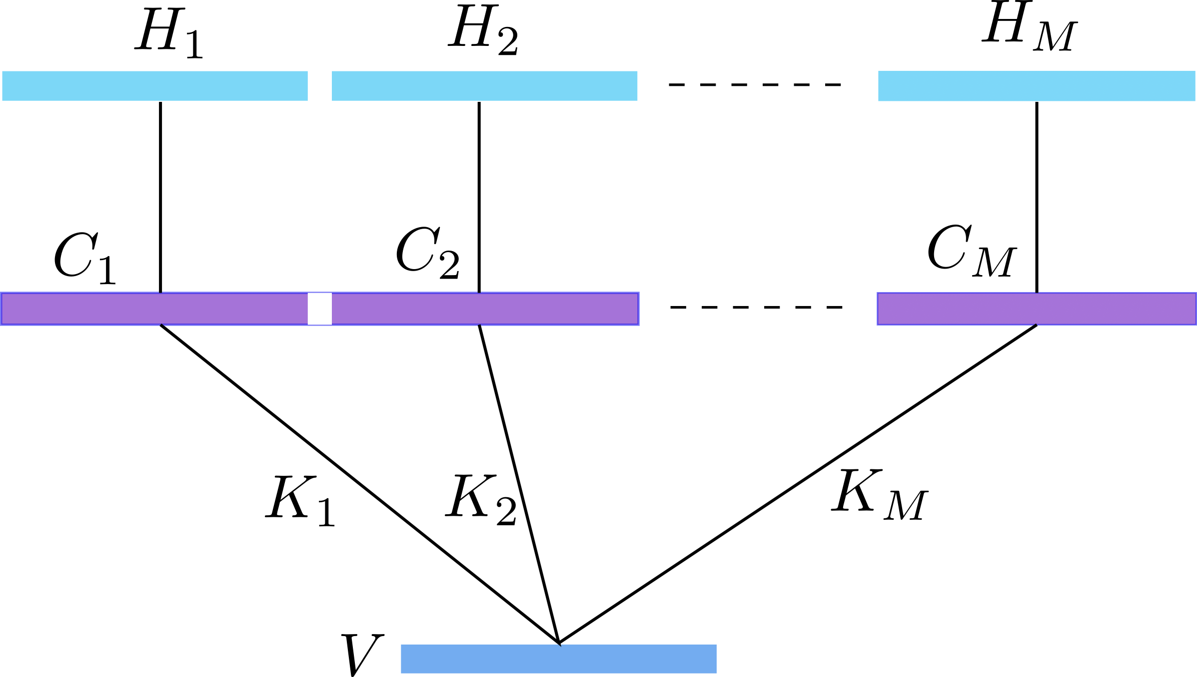
Figure 2: Schematic diagram of a CRBM network. The visible layer ($V$) contains $N_{v}=2L$ neurons as in RBM. The hidden layer is enlarged compared to RBM and consists of $M$ blocks $H_{1},\,H_{2},\,\ldots,H_{M}$, each containing $N_{v}$ neurons. There is a convolutional layer in between which also consists of $M$ blocks $C_{1},\,C_{2},\,\ldots,C_{M}$. The $m$-th block applies a convolutional filter with kernel $K_{m}$ to the visible layer and generates an output which is in the form of $N_{v}$ output neurons comprising the $C_{m}$ block. There are one-to-one connections between the neurons in the $C_{m}$ and $H_{m}$ blocks.

It can be thought of as consisting of three layers with an additional convolutional layer in between the visible and the hidden layersNorouzi (2009); Alcalde Puente and Eremin (2020). Since the underlying lattice is two-dimensional (2D), it is necessary to consider layers also to be 2D arrays of neurons instead of the linear arrangement of Fig. 1. The visible layer again contain $N_{v}=2L$ neurons, like in RBM. But the hidden layer ($H$ layer) in CRBM is enlarged to make it into $M$ blocks $H_{1},\,H_{2}\,\ldots,H_{M}$, each block containing $N_{h}=N_{v}$ neurons. The middle convolutional layer ($C$ layer) also consists of $M$ blocks $C_{1},\,C_{2},\,\ldots,\,C_{M}$. The input layer, the blocks $C_{m}$-s, $H_{m}$-s are all taken to be $2P\times P$ arrays of neurons, where $P=\sqrt{L}$. The $m$-th block applies a convolution filter with kernel $K_{m}$ to the input layer and produces a result which is in the form of $N_{v}$ number of convolutional output neurons ($2P\times P$ array) comprising the $C_{m}$ block. The convolutional output blocks are connected directly to the hidden layer blocks. That is, the $i$-th neuron in $m$-th convolutional block is connected only to the $i$-th neuron of the $m$-th hidden layer block, and not to any other hidden unit. Thus, there is a one-to-one connection between the neurons in the blocks $C_{m}$ and $H_{m}$, with a total of $N_{v}$ connections between the two sub-layers. Therefore for $M\ll L$, the total number of connections in the CRBM is much less compared to that in the RBM, making the CRBM representation much more efficient in comparison.

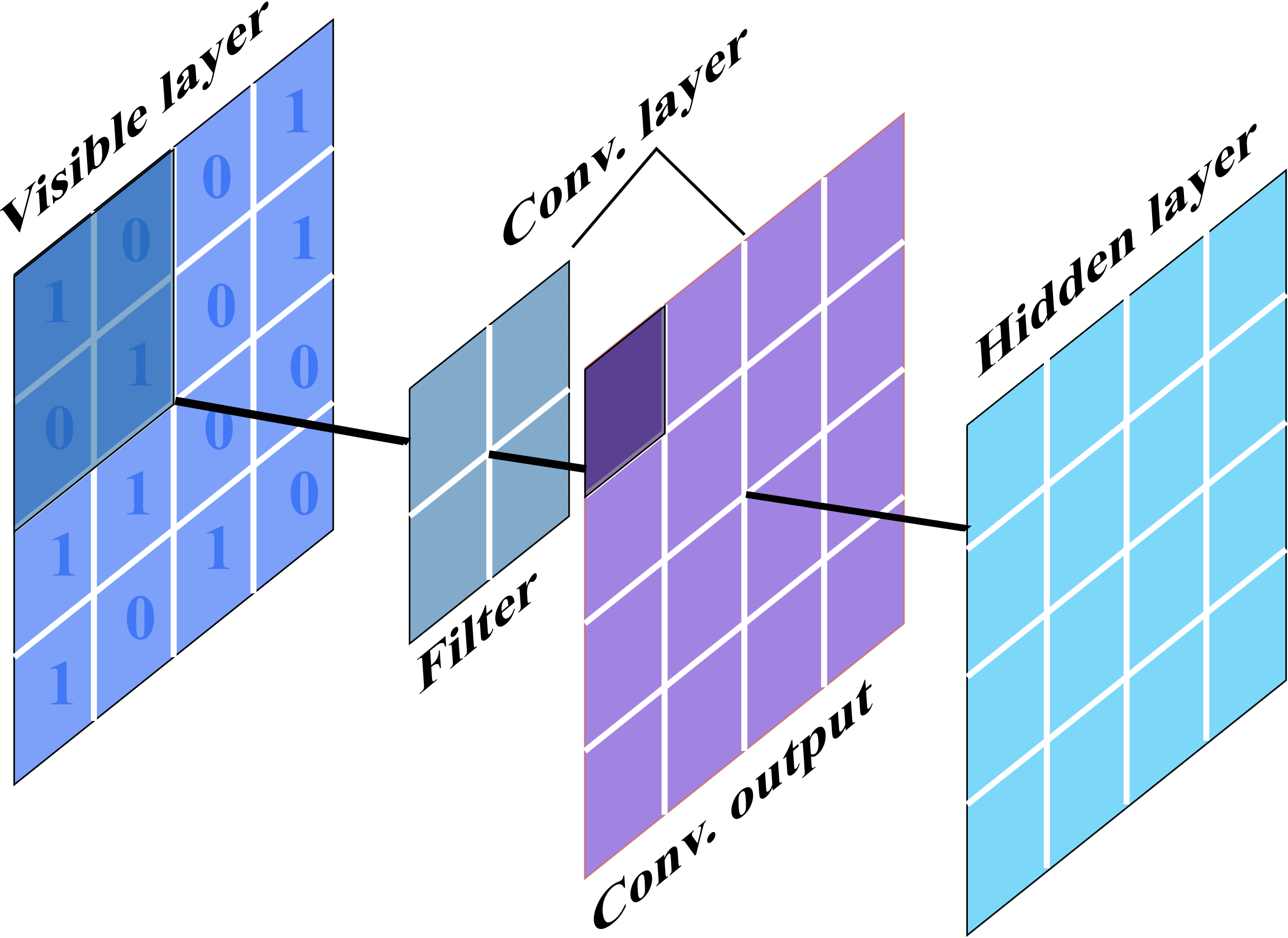
Figure 3: Schematic diagram showing the convolutional operation by one of the $C$-blocks in Fig. 2. The convolutional layer slides a filter over the visible layer with a stride of one. The operation generates the convolutional output layer which is of the same dimension as the input layer.

Next, consider the convolutional operation by the $m$-th block (Fig. 3). The convolutional filter in the block is defined by its kernel $K_{m}$ which is a matrix of $D\times D$ parameters ($D\leq P$). Action of the filter on a $D\times D$ window of the visible layer is given by the generalized dot product $K_{m}\odot V_{k}$, where $V_{k}$ is the matrix formed by the input values given to the neurons in this window. This is shown schematically in Fig. 3. We slide the filter with a stride of one step along both the directions to cover the whole of the visible layer. This creates $N_{v}$ number of windows of the visible layer and hence $N_{v}$ number of convolutional outputs $K_{m}\odot V_{k}$, $k=1,\,2,\,\ldots N_{v}$. Denoting the $i$-th hidden variable in the $m$-th block by $h_{mi}$, the joint energy function in the CRBM is given by,

$$E_{CRBM}=-\sum_{m,k}h_{mk}(K_{m}\odot V_{k})-a\sum_{j}n_{j}-\sum_{mi}b_{m}h_{mi}$$ (5)

It may be mentioned that by construction CRBM conservs the lattice translational symmetry imposed in the corresponding RBM. The probability distribution over the visible variables in CRBM is given by,

$$\Psi_{CRBM}= \frac{1}{Z}\sum_{\bf h}e^{-E_{CRBM}}$$

$$= \frac{1}{Z}e^{a\sum_{j}n_{j}}\prod_{mk}2\cosh\left(K_{m}\odot V_{k}+b_{m}\right)$$ (6)

where $Z$ is a normalization constant. The total number of parameters in the CRBM is $M(2D^{2}+1)$. This number depends only upon the two network structural parameters $M$ and $D$, and not upon the lattice size, $L$. Therefore the number of variational parameters in the CRBM wave function does not grow directly with the lattice size which is a big advantage in the optimization process. In practice, the parameters $M$ and $D$ are determined by tuning its values so as to obtain the best variational energy. The lattice size might affect these values somewhat, but the number of variational parameters is still expected to be much less than that in the corresponding RBM wave function.

II.3 CRBM correlated wave function

The CRBM correlated wave function that we consider here is given by,

$$|\Psi_{var}\rangle={\cal P}_{CRBM}\ket{BCS}_{N}$$ (7)

where $\ket{BCS}_{N}$ is the ground state (with fixed number of particles) of the following mean-field Hamiltonian,

$${\cal H}_{MF}= \sum_{\mathbf{k}\sigma}\varepsilon_{\mathbf{k}}c^{\dagger}_{\mathbf{k}\sigma}c_{\mathbf{k}\sigma}-\sum_{\mathbf{k}}\left(\Delta_{\mathbf{k}}c^{{\dagger}}_{\mathbf{k}\uparrow}c^{{\dagger}}_{-\mathbf{k}\downarrow}+hc\right)$$ (8)

Here $\varepsilon_{\mathbf{k}}=-2t(\cos k_{x}+\cos k_{y})+4t^{\prime}\cos k_{x}\cos k_{y}-\mu$, $\mu$ being the chemical potential. We take superconducting pairing amplitude $\Delta_{\mathbf{k}}$ to be of $d_{x^{2}-y^{2}}$-wave ($d$-wave) symmetry with $\Delta_{\mathbf{k}}=\Delta_{SC}(\cos k_{x}-\cos k_{y})$, where $\Delta_{SC}$ is the SC gap parameter. The quantities $\Delta_{SC}$ and $\mu$ are the variational parameters in the one-body part of the wave function. We consider the wave function in fixed particle number ($2N$) representation with equal number of up and down spins. In terms of real-space (Wannier) basis, $\ket{BCS}_{N}$ can be expressed as,

$$\ket{BCS}_{N}= \sum_{n_{1},n_{2},\ldots n_{2L}}\Psi_{BCS}(n_{1},n_{2},\ldots n_{2L})$$

$$\times(c^{{\dagger}}_{1\uparrow})^{n_{1}}\ldots(c^{{\dagger}}_{L\uparrow})^{n_{L}}(c^{{\dagger}}_{1\downarrow})^{n_{L+1}}\ldots(c^{{\dagger}}_{L\downarrow})^{n_{2L}}\ket{0}$$

$$= \sum_{R}\Psi_{BCS}(R)\ket{R}$$ (9)

Here $n_{i}$-s are the occupation numbers which can take value $0$ or $1$. $L$ is the number of lattice sites. The summation is over the set of values $\{n_{1},\ldots n_{2L}\}\equiv R$ subject to constraint $\sum_{i=1}^{L}n_{i}=\sum_{i={L+1}}^{2L}n_{i}=N$. The amplitudes $\Psi_{BCS}(R)$-s are the determinantal coefficients corresponding to the electronic configurations. The action of ${\cal P}_{CRBM}$ is given by,

$$\ket{\Psi_{var}}={\cal P}_{CRBM}\ket{\Phi}=\sum_{R}\Psi_{CRBM}(R)\Psi_{BCS}(R)\ket{R}$$ (10)

where $\Psi_{CRBM}(R)$ is output (Eq. (6)) of the CRBM network for a given set of input values $R=\{n_{1},\ldots n_{2L}\}$. The variational parameters in the wave function consists of the network parameters plus the parameters in the mean-field part of the wave function.

II.4 Variational Monte Carlo

Having constructed the variational wave function, we use the variational Monte Carlo (VMC) methodCeperley et al. (1977); Sorella (2013); Tahara and Imada (2008) to compute the variational energy,

$$E_{var}(\bm{\alpha})=\frac{\bra{\Psi_{var}}{{\cal H}}\ket{\Psi_{var}}}{\bra{\Psi_{var}}\Psi_{var}\rangle}$$ (11)

and minimize it with respect to the variational parameters $\bm{\alpha}$. We use the stochastic reconfiguration (SR) techniqueSorella (2013); Tahara and Imada (2008) for optimization which generally works all even for large number of variational parameters. In this method, the variational parameters $\bm{\alpha}$ are updated as, $\bm{\gamma}=\bm{\alpha}-\Delta tS^{-1}\mathbf{g}$ where $\mathbf{g}=\bm{\nabla}_{\alpha}E_{var}$ is the energy gradient. $S$ is the overlap matrix with the matrix elements given by, $S_{kl}=\langle\Psi_{\alpha_{k}}\ket{\Psi_{\alpha_{l}}}$, $\ket{\Psi_{\alpha_{k}}}=\frac{\partial}{\partial\alpha_{k}}\ket{\Psi_{\bm{\alpha}}}$. In the VMC simulations, typically we take $\sim 10^{5}$ measuring steps after warming up the system for $\sim 10^{3}$ steps. Each MC step consists of $L$ number of MC moves that include both the hopping and exchange moves as mentioned before. The number of variational parameters in the CRBM wave function depends upon the two network structural parameters $M$ and $D$, and independent of the lattice size. For the values of $M$ and $D$ considered here, the number of variational parameters becomes of the order of 150. The optimization step even with the SR method sometime does need large number of iterations to converge which creates a bottleneck in the computations.

III Results

We consider the Hamiltonian on a square lattice of size $10\times 10$ with $L=100$ sites, and a band filling of one particle per site (half-filling). We consider two values of the next-nearest hopping parameter $t^{\prime}$, e.g. $t^{\prime}/t=0$ and $t^{\prime}/t=0.5$. The non-zero value $t^{\prime}/t$ brings in frustration in the antiferromagnetic order expected at half-filling. We study the model as a function of Hubbard onsite interaction $U/t$. In the results below, all the energy values quoted are energy per site and in units of $t$.

Before going ahead with the calculations, we need to determine the optimal configuration of the CRBM network. It has two crucial structural parameters - the dimension $D$ of the convolutional kernel and the number of convolution blocks $M$. In principle, $D$ can vary from 1 to $L$. The convolution can be interpreted as a ‘feature extraction’ operationNorouzi (2009). A value $D=1$ implies a trivial operation while $D=L$ implies flattening of all features. Here we take $D=4$ which we find to be an optimal value in terms of performance and efficiency. Regarding value of $M$, we checked the energy obtained by repeating the optimizations for different values of $M$. An example plot is shown in Fig. 4.

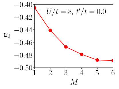
Figure 4: Energy obtained by repeating optimizations for different values of the CRBM parameter $M$. The energy reaches a saturation value at $M\sim 5$. The value of the parameter $D$ is 4. Model parameters, $U/t=8$ and $t^{\prime}/t=0$.

It shows that at $U/t=8$, the best energy is obtained for a minimum $M$ value of $5$. In fact, the optimal value of $M$ depends upon the value of $U$. It is smaller for smaller $U$. Therefore, a value of $5$ works well for the range of $U/t$ considered here and hence we set $M=5$ for the rest of the calculations.

We optimize the CRBM wave function defined in Eq. (10) by minimizing the corresponding variational energy for a range of model parameter values. For comparison, we also calculate the energies of four other variational wave functions. These are (i) $\ket{\Psi_{GW}}={\cal P}_{G}\ket{BCS}_{N}$ (GW) (ii) $\ket{\Psi_{GW+DH}}={\cal P}_{G}{\cal P}_{DH}\ket{BCS}_{N}$ (GW+DH) (iii) $\ket{\Psi_{Jastrow}}={\cal P}_{J}\ket{BCS}_{N}$ (Jastrow) and (iv) $\ket{\Psi_{RBM}}={\cal P}_{RBM}\ket{BCS}_{N}$ (RBM), where the projection operators are as defined above. In $\ket{\Psi_{RBM}}$, we use an RBM network as the correlator. The comparison of energies of these wave functions are shown in Fig. 5.

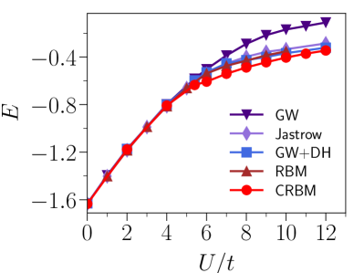
(a)

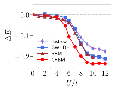
(b)

Figure 5: (a) Energies of the five wave functions described in the text as a function of $U/t$. (b) The difference $\Delta E=E_{X}-E_{GW}$, where $X$ stands for the four wave function names shown in the figure.

It shows that, in the weak coupling limit, the energies of these WFs are more or less similar with minor differences among them. However, the energies start to differ in the strong coupling regime. This is clear from Fig. 5(b) where we have plotted the difference $\Delta E=E_{X}-E_{GW}$, where $X$ stands for the four other wave functions shown in the figure. As the figure shows, $\Delta E$ is negative in the intermediate to strong coupling regime, indicating that the energy of the GW wave function is highest here. The energies of the GW+DH and RBM wave functions are comparable and lower than that of the Jastrow wave function. The best wave function among the five is the CRBM wave function which yields energies significantly lower than the other four. We also compare the CRBM energies with those for the long range backflow-Jastrow correlated wave function used in Ref. Tocchio et al., 2011, which was shown to be the most accurate among the Jastrow type projected wave functions. We find that the CRBM wave function even outperforms the backflow-Jastrow wave function. For example, the backflow WF give energies per site equal to $-0.5961(1)$, $-0.4803(1)$, $-0.4022(1)$ and $-0.3451(1)$ at $U/t$ equal to $6$, $8$, $10$, and $12$, respectively. For the same values of $U/t$, the CRBM wave function give energies per site equal to $-0.6076(2)$, $-0.4882(2)$, $-0.4048(2)$, and $-0.3456(2)$, respectively. These energies are clearly lower than the backflow WF energies. It must be mentioned that the lattice sizes used in these two studies are not the same, and hence the comparison is not strictly rigorous. Still, it gives an idea about how accurate the CRBM wave function is. In Ref. Nomura et al., 2017, the authors used an RBM correlator in conjunction with a many-variable one-body wave function. The energies of this wave function is actually lower than the CRBM energies, though such a wave function is computationally much more expensive.

Next, we examine the ground state phase of the model as a function of $U/t$ as described by the CRBM wave function. As mentioned before, we have done calculations for two different values of $t^{\prime}$, e.g. $t^{\prime}/t=0$ and $t^{\prime}/t=0.5$. Although the model has been studied extensively in the past using a variety of methods, several important aspects of its phase diagram including the nature of the zero temperature Mott transition, are not yet established unambiguouslySchäfer et al. (2015); LeBlanc et al. (2015); Mukherjee and Lal (2020). For example, questions exist whether the ground state of the unfrustrated model ($t^{\prime}/t=0$) on square lattice is antiferromagnetic (AF) insulating at any $U/t>0$, or is it paramagnetic with a finite value of critical interaction $U_{c}/t$ for Mott metal-insulator transition. What is the nature of Mott insulating state, is it magnetically ordered or a spin liquid? If the unfrustrated model is AF insulating, is there a critical value of $t^{\prime}$ beyond which the ground state become paramagnetic metallic? The answers to these questions somewhat vary among different methods. Within the variational theory, the phase diagram of the two-dimensional Hubbard model has been studied by looking at the competition between wave functions with different symmetries. In these wave functions, the one-body part is taken to be either pure BCS type without any magnetic order or an AF type with explicitly broken spin rotational symmetry. By using the GW-DH projector as the correlator, Yokoyama et al.Yokoyama et al. (2006) have shown that at $t^{\prime}=0$, the lowest energy state at any $U/t>0$ is the symmetry broken one with long range AF order and insulating. For $t^{\prime}/t>0$, there exists a non-zero value of critical interaction $U_{c}$ below which the state is paramagnetic metallic (PM). For $U/t>U_{c}/t$, the state is AF insulating for small $t^{\prime}/t$, but paramagnetic insulating at large $t^{\prime}/t$. The transition to the AF insulating state at $t^{\prime}/t=0$ is continuous. It gradually turns first-order at larger $t^{\prime}/t$. However, if considered within the non-magnetic projected BCS wave function only, the state is found to be PM for any $t^{\prime}/t$ below a critical $U_{c}/t\neq 0$. In this case, the Mott transition is of first-order nature at any $t^{\prime}/t$, and the insulating state is non-magnetic. In another work, Tocchio et alTocchio et al. (2008) used variational WFs with backflow correlations in addition to a long range Jastrow projector. The backflow correlated WFs is much more accurate with lower variational energy compared to only DH or Jastrow projected WFs. The study also showed that for small $U/t$ and non-zero $t^{\prime}/t$, the ground is paramagnetic metallic. It becomes insulating with a long range AF order as $U$ is increased above a critical value. Interestingly, the backflow WF give a region in the phase diagram at large enough values of $U/t$ and $t^{\prime}/t$, where the state is insulating spin-liquid without any long range magnetic order.

In contrast to the above studies which considered wave functions with different symmetries, here we study the ground state within the single variational wave function. We show that, though no magnetic order is put explicitly into the CRBM+BCS wave function, it spontaneously gives rise to long range AF order in the insulating state. This is remarkable as this was not observed with any of the other variational WFs considered in the previous studies. In order to characterize the ground state, first we compute the doublon-holon (DH) correlation function defined as,

$$C_{ij}(r)=\frac{\langle d_{i}h_{j}\rangle-\langle d_{i}\rangle\langle h_{j}\rangle}{\langle d_{i}\rangle\langle h_{j}\rangle}$$ (12)

where $d_{i}=n_{i\uparrow}n_{i\downarrow}$ and $h_{i}=(1-n_{i\uparrow})(1-n_{i\downarrow})$ are the doublon and holon operator, respectively. The results for the nearest-neighbor (NN) and next-nearest-neighbor (NNN) correlations as a function of $U$ are shown in Fig. 6.

(a)

(b)

Figure 6: Doublon-holon correlations at (a) nearest-neighbor and (b) next-nearest-neighbor distances as a function of $U/t$. Results are shown for two values of $t^{\prime}/t$.

It shows that $C_{ij}(r)$ is very close to zero at small $U/t$. As $U/t$ is increased, it shows a jump at a critical $U_{c}/t$ and steadily rises after. The NNN values are an order of magnitude smaller than the NN values, indicating the bindings of doublons and holons within short distances from each other. Thus the wave function is able to capture the correct physics of doulon-holon bindings in the strong coupling regime in spite of it not having any explicit doublon-holon correlation factor. Next, we compute the double occupancy, $D$ defined as

$$D=\frac{1}{N_{\mathrm{s}}}\sum_{i}n_{i\uparrow}n_{i\downarrow}$$ (13)

It is a crucial quantity that can indicate the presence of Mott transition. The value of $D$ is shown in Fig. 7.

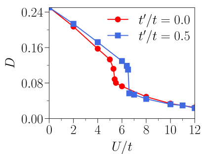
Figure 7: Double occupancy $D$ as a function of $U/t$ at the two values of $t^{\prime}$ shown.

Starting from a value of $0.25$ at $U/t=0$, $D$ decreases as $U/t$ is increased. It shows a sudden drop at a critical $U_{c}/t$ indicating the onset of Mott transition. The jump in the value of $D$ is clearly present at both the values of $t^{\prime}$, though it is sharper in the frustrated case. It may be mentioned that, even in the long ranged backflow correlated WF used in previous studiesTocchio et al. (2011), the $D$ at Mott transition at $t^{\prime}/t=0$ shows only a kink not a jump. We find that the values of critical interaction are $U_{c}/t\sim 5.4$ for $t^{\prime}/t=0$ and $U_{c}/t\sim 6.6$ for $t^{\prime}/t=0.5$. These values are in roughly in good agreement with previous resultsYokoyama et al. (2006); Tocchio et al. (2008). The occurence of Mott transition can be confirmed directly by looking at the charge gap which can be estimated from the knowledge of the ground state WF itself. Given the ground state $\ket{\Psi}$, an excited state with momentum $\mathbf{q}$ is given by $n_{\mathbf{q}}\ket{\Psi}$, and the charge gap in limit $q\rightarrow 0$ for square lattice can be shown to beTocchio et al. (2011),

$$E_{g}=-\frac{1}{4}\left(\lim_{q\rightarrow 0}\frac{|\mathbf{q}|^{2}}{N(\mathbf{q})}\right)\left({\cal K}_{1}+2{\cal K}_{2}\right)$$ (14)

where $N(\mathbf{q})=\langle n_{\mathbf{q}}n_{-\mathbf{q}}\rangle$ is the charge structure factor. ${\cal K}_{1}$ and ${\cal K}_{2}$ are the NN and the NNN kinetic energy per site, respectively. The results for $E_{g}$ are shown in Fig. 8.

Figure 8: Charge gap $E_{g}$ as a function of $U/t$.

It confirms that the state below $U_{c}/t$ is metallic with no charge gap, while above $U_{c}/t$ it is insulating with a finite charge gap. Next we look at the momentum distribution function, $n(\mathbf{k})=\langle c^{\dagger}_{k\sigma}c_{k\sigma}\rangle$. The $n(\mathbf{k})$ values calculated as a function of $\mathbf{k}$ along the symmetry path $\Gamma(0,0)$-$X(\pi,0)$-$M(\pi,\pi)$-$\Gamma(0,0)$ for different values of $U/t$ for the case $t^{\prime}/t=0$ are shown in Fig. 9(a). In the metallic state, $n(\mathbf{k})$ has a discontinuity at the Fermi surface, $k=k_{F}$ in the nodal $\Gamma-M$ direction. The magnitude of the jump gives the quasiparticle weight $Z$ which roughly corresponds to the inverse effective mass of the quasiparticlesParamekanti et al. (2004); Yokoyama et al. (2006). We plot the values of $Z$ so determined as a function of $U/t$ in Fig. 9(a). For both the cases of $t^{\prime}/t$, $Z$ decreases with increasing $U/t$ and show a sudden drop at the respective critical interaction $U_{c}/t$. Interestingly, $Z$ does not vanish completely in the Mott state for the unfrustrated case at $t^{\prime}/t=0$, though it becomes very small. Thus it suggests that the Mott transition in this case takes place via vanishing of spectral weight at the Fermi level rather than via divergence of effective mass. In contrast, $Z$ vanishes completely in the Mott state for $t^{\prime}/t=0.5$ case suggesting divergence of the effective mass in this case. For both the cases, the transition is found to be first-order nature as evidenced from discontinuities of various quantities at the critical point.

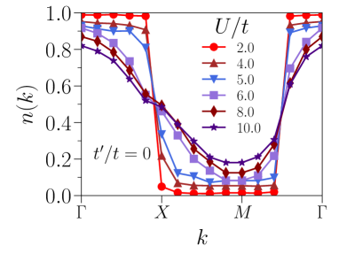
(a)

(b)

Figure 9: (a) Momentum distribution at various values of $U/t$ along the symmetry path in the first Brillouin zone ($t^{\prime}/t=0$). (b) Quasiparticle weight $Z$ determined from the jump at the Fermi surface, as a function of $U/t$, for the two cases of $t^{\prime}/t$.

Finally, we look at the magnetic correlations in the CRBM wave function. We calculate the spin structure factor $S(\mathbf{q})$ defined as,

$$S(\mathbf{q})=\frac{1}{L^{2}}\sum_{i,j}e^{i\mathbf{q}\cdot(\mathbf{r}_{i}-\mathbf{r}_{j})}\langle S^{z}_{i}S^{z}_{j}\rangle$$ (15)

where $S^{z}_{i}=(n_{i\uparrow}-n_{i\downarrow})$ is the $z$-component of the spin operator at site $i$. The results for $S(\mathbf{q})$ calculated at various values of $U/t$ are shown in Fig. 10.

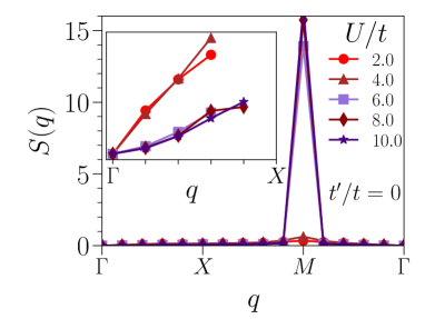
(a)

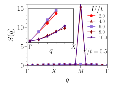
(b)

Figure 10: Spin structure factor $S(\mathbf{q})$ as a function of $\mathbf{q}$ at various values of $U/t$ for the cases (a) $t^{\prime}/t=0$ and (b) $t^{\prime}/t=0.5$. The inset in each case show $S(\mathbf{q})$ versus $\mathbf{q}$ for small $|\mathbf{q}|$. It shows that in the limit $|\mathbf{q}|\rightarrow 0$, $S(\mathbf{q})\propto|\mathbf{q}|$ for $U<U_{c}$ (gapless), while $S(\mathbf{q})\propto|\mathbf{q}|^{2}$ for $U>U_{c}$ (spin gap).

As the figure shows, $S(\mathbf{q})$ is very small at all $\mathbf{q}$ for $U<U_{c}$ indicating very weak magnetic correlations in the metallic state. For $U>U_{c}$, $S(\mathbf{q})$ is very sharply peaked at $\mathbf{q}=(\pi,\pi)$ which indicates onset on long range AF correlations as soon as the system enters the Mott state. The non-zero values of $t^{\prime}$ considered here does not seem have any impact on the AF correlations. In fact, we find that the sublattice magnetization $m=|S^{z}_{i}|$ which is close zero in the metallic phase, jumps to around $0.8$ at transition, a value close to the saturation limit. If we compare with results in Ref. Yokoyama et al., 2006, the AF correlations in the insulating state in the GW+DH wave function used in this study is much weaker compared to what is found here. The insets in the figures show $S(\mathbf{q})$ for a small range of $|\mathbf{q}|$. Clearly in the limit $|\mathbf{q}|\rightarrow 0$, the $S(\mathbf{q})\propto|\mathbf{q}|$ in the metallic phase suggesting absence of spin gap in this phase. On the other hand, $S(\mathbf{q})\propto|\mathbf{q}|^{2}$ for $U>U_{c}$ suggesting that the Mott state is also spin gapped.

IV Conclusion

In summary, we have studied the ground state phase of the half-filled Hubbard model on a square lattice using a variational wave function which is constructed by applying a convolutional restricted Boltzmann machine (CRBM) neural network as correlator to a mean-field BCS wave function. The number of variational parameters in the wave function does not automatically grow with the lattice size and can be tuned. The wave function is also highly accurate, especially in the strong coupling limit where it yields variational energies lower than those of the best known Jastrow variational WFs for the model. The picture of Mott metal-insulator transition in the model as described by the CRBM wave function is roughly similar to that obtained by using other variational wave functionsYokoyama et al. (2006); Tocchio et al. (2008, 2011), with some interesting differences. Regarding the shortcomings of the CRBM wave function, the results for the energies shows that the it does not necessarily perform better in the weak coupling limit. Other more accurate methods strongly suggest that for the unfrustrated model with $t^{\prime}/t=0$, there exist short range AF fluctuations even in the weak coupling limit and the ground state in this case is insulating at all $U_{c}/t>0$Schäfer et al. (2015); LeBlanc et al. (2015); Mukherjee and Lal (2020). This physics is not captured correctly in the CRBM wave function. This of course can be remedied readily by putting an AF order manually into the mean-field part of the wave function, though it would be much desirable to have the correlations generated spontaneously in the same manner as in the Mott insulating state. It is also interesting to study the wave function for a range of $t^{\prime}/t$ values in order to obtain a full phase diagram as a function of $U/t$ and $t^{\prime}/t$. We leave it for a future study.

References

- Imada et al. (1998) M. Imada, A. Fujimori, and Y. Tokura, Rev. Mod. Phys. 70, 1039 (1998).
- LeBlanc et al. (2015) J. P. F. LeBlanc, A. E. Antipov, F. Becca, I. W. Bulik, G. K.-L. Chan, C.-M. Chung, Y. Deng, M. Ferrero, T. M. Henderson, C. A. Jiménez-Hoyos, E. Kozik, X.-W. Liu, A. J. Millis, N. V. Prokof’ev, M. Qin, G. E. Scuseria, H. Shi, B. V. Svistunov, L. F. Tocchio, I. S. Tupitsyn, S. R. White, S. Zhang, B.-X. Zheng, Z. Zhu, and E. Gull (Simons Collaboration on the Many-Electron Problem), Phys. Rev. X 5, 041041 (2015).
- Lee et al. (2006a) P. A. Lee, N. Nagaosa, and X.-G. Wen, Rev. Mod. Phys. 78, 17 (2006a).
- Ceperley et al. (1977) D. Ceperley, G. V. Chester, and M. H. Kalos, Phys. Rev. B 16, 3081 (1977).
- Tahara and Imada (2008) D. Tahara and M. Imada, Journal of the Physical Society of Japan 77, 114701 (2008), https://doi.org/10.1143/JPSJ.77.114701 .
- Sorella (2013) S. Sorella, in Strongly Correlated Systems, Springer Series in Solid-State Sciences, Vol. 176, edited by A. Avella and F. Mancini (Springer, Berlin, Heidelberg, 2013) Chap. Variational Monte Carlo and Markov Chains for Computational Physics.
- Paramekanti et al. (2004) A. Paramekanti, M. Randeria, and N. Trivedi, Phys. Rev. B 70, 054504 (2004).
- SHIBA and YOKOYAMA (1987) H. SHIBA and H. YOKOYAMA, in Proceedings of the Yamada Conference XVIII on Superconductivity in Highly Correlated Fermion Systems, edited by M. Tachiki, Y. Muto, and S. Maekawa (Elsevier, 1987) pp. 264–267.
- Carrasquilla and Melko (2017) J. Carrasquilla and R. G. Melko, Nature Physics 13, 431–434 (2017).
- Carleo and Troyer (2017) G. Carleo and M. Troyer, Science 355, 602–606 (2017).
- van Nieuwenburg et al. (2017) E. P. L. van Nieuwenburg, Y.-H. Liu, and S. D. Huber, Nature Physics 13, 435–439 (2017).
- Broecker et al. (2017) P. Broecker, J. Carrasquilla, R. G. Melko, and S. Trebst, Scientific Reports 7, 8823 (2017).
- Ch’ng et al. (2017) K. Ch’ng, J. Carrasquilla, R. G. Melko, and E. Khatami, Phys. Rev. X 7, 031038 (2017).
- Deng et al. (2017) D.-L. Deng, X. Li, and S. Das Sarma, Phys. Rev. X 7, 021021 (2017).
- Carleo et al. (2019) G. Carleo, I. Cirac, K. Cranmer, L. Daudet, M. Schuld, N. Tishby, L. Vogt-Maranto, and L. Zdeborová, Rev. Mod. Phys. 91, 045002 (2019).
- Carrasquilla (2020) J. Carrasquilla, Advances in Physics: X 5, 1797528 (2020), https://doi.org/10.1080/23746149.2020.1797528 .
- Melko et al. (2019) R. G. Melko, G. Carleo, J. Carrasquilla, and J. I. Cirac, Nature Physics 15, 887 (2019).
- Carrasquilla and Torlai (2021) J. Carrasquilla and G. Torlai, PRX Quantum 2, 040201 (2021).
- Torlai et al. (2018) G. Torlai, G. Mazzola, J. Carrasquilla, M. Troyer, R. Melko, and G. Carleo, Nature Physics 14, 447–450 (2018).
- Carleo et al. (2018) G. Carleo, Y. Nomura, and M. Imada, Nature Communications 9, 5322 (2018).
- Choo et al. (2018) K. Choo, G. Carleo, N. Regnault, and T. Neupert, Phys. Rev. Lett. 121, 167204 (2018).
- Lu et al. (2019) S. Lu, X. Gao, and L.-M. Duan, Phys. Rev. B 99, 155136 (2019).
- Glasser et al. (2018) I. Glasser, N. Pancotti, M. August, I. D. Rodriguez, and J. I. Cirac, Phys. Rev. X 8, 011006 (2018).
- Zhang and Weng (2014) L. Zhang and Z.-Y. Weng, Phys. Rev. B 90, 165120 (2014).
- Cai and Liu (2018) Z. Cai and J. Liu, Phys. Rev. B 97, 035116 (2018).
- Nomura et al. (2017) Y. Nomura, A. S. Darmawan, Y. Yamaji, and M. Imada, Phys. Rev. B 96, 205152 (2017).
- Inui et al. (2021) K. Inui, Y. Kato, and Y. Motome, Phys. Rev. Res. 3, 043126 (2021).
- Luo and Clark (2019) D. Luo and B. K. Clark, Phys. Rev. Lett. 122, 226401 (2019).
- Pfau et al. (2020) D. Pfau, J. S. Spencer, A. G. D. G. Matthews, and W. M. C. Foulkes, Phys. Rev. Res. 2, 033429 (2020).
- MOTT (1968) N. F. MOTT, Rev. Mod. Phys. 40, 677 (1968).
- Orenstein and Millis (2000) J. Orenstein and A. J. Millis, Science 288, 468 (2000).
- Lee et al. (2006b) P. A. Lee, N. Nagaosa, and X.-G. Wen, Rev. Mod. Phys. 78, 17 (2006b).
- Georges et al. (1996) A. Georges, G. Kotliar, W. Krauth, and M. J. Rozenberg, Rev. Mod. Phys. 68, 13 (1996).
- Zhang et al. (1993) X. Y. Zhang, M. J. Rozenberg, and G. Kotliar, Phys. Rev. Lett. 70, 1666 (1993).
- Rozenberg et al. (1994) M. J. Rozenberg, G. Kotliar, and X. Y. Zhang, Phys. Rev. B 49, 10181 (1994).
- Park et al. (2008) H. Park, K. Haule, and G. Kotliar, Phys. Rev. Lett. 101, 186403 (2008).
- Rozenberg et al. (1999) M. J. Rozenberg, R. Chitra, and G. Kotliar, Phys. Rev. Lett. 83, 3498 (1999).
- Bulla et al. (2001) R. Bulla, T. A. Costi, and D. Vollhardt, Phys. Rev. B 64, 045103 (2001).
- Lu (1994) J. P. Lu, Phys. Rev. B 49, 5687 (1994).
- Ferrero et al. (2005) M. Ferrero, F. Becca, M. Fabrizio, and M. Capone, Phys. Rev. B 72, 205126 (2005).
- Rüegg et al. (2005) A. Rüegg, M. Indergand, S. Pilgram, and M. Sigrist, Eur. Phys. J. B 48, 55 (2005).
- Mukherjee and Lal (2020) A. Mukherjee and S. Lal, New Journal of Physics 22, 063007 (2020).
- Yokoyama and Shiba (1990) H. Yokoyama and H. Shiba, Journal of the Physical Society of Japan 59, 3669 (1990), https://doi.org/10.1143/JPSJ.59.3669 .
- Yokoyama et al. (2006) H. Yokoyama, M. Ogata, and Y. Tanaka, Journal of the Physical Society of Japan 75, 114706 (2006).
- Capello et al. (2005) M. Capello, F. Becca, M. Fabrizio, S. Sorella, and E. Tosatti, Phys. Rev. Lett. 94, 026406 (2005).
- Capello et al. (2006) M. Capello, F. Becca, S. Yunoki, and S. Sorella, Phys. Rev. B 73, 245116 (2006).
- Tocchio et al. (2008) L. F. Tocchio, F. Becca, A. Parola, and S. Sorella, Phys. Rev. B 78, 041101 (2008).
- Tocchio et al. (2011) L. F. Tocchio, F. Becca, and C. Gros, Phys. Rev. B 83, 195138 (2011).
- Kaplan et al. (1982) T. A. Kaplan, P. Horsch, and P. Fulde, Phys. Rev. Lett. 49, 889 (1982).
- Norouzi (2009) M. Norouzi, Convolutional restricted boltzmann machines for feature learning, Master’s thesis, School of Computing Science, Simon Fraser University (2009).
- Alcalde Puente and Eremin (2020) D. Alcalde Puente and I. M. Eremin, Phys. Rev. B 102, 195148 (2020).
- Schäfer et al. (2015) T. Schäfer, F. Geles, D. Rost, G. Rohringer, E. Arrigoni, K. Held, N. Blümer, M. Aichhorn, and A. Toschi, Phys. Rev. B 91, 125109 (2015).