Stable and Robust Deep Learning By Hyperbolic Tangent Exponential Linear Unit (TeLU)

Abstract

In this paper, we introduce the Hyperbolic Tangent Exponential Linear Unit (TeLU), a novel neural network activation function, represented as $f(x)=x{\cdot}tanh(e^{x})$. TeLU is designed to overcome the limitations of conventional activation functions like ReLU, GELU, and Mish by addressing the vanishing and, to an extent, the exploding gradient problems. Our theoretical analysis and empirical assessments reveal that TeLU outperforms existing activation functions in stability and robustness, effectively adjusting activation outputs’ mean towards zero for enhanced training stability and convergence. Extensive evaluations against popular activation functions (ReLU, GELU, SiLU, Mish, Logish, Smish) across advanced architectures, including Resnet-50, demonstrate TeLU’s lower variance and superior performance, even under hyperparameter conditions optimized for other functions. In large-scale tests with challenging datasets like CIFAR-10, CIFAR-100, and TinyImageNet, encompassing 860 scenarios, TeLU consistently showcased its effectiveness, positioning itself as a potential new standard for neural network activation functions, boosting stability and performance in diverse deep learning applications.

1 Introduction

In the rapidly evolving landscape of neural networks, the choice of activation function plays a pivotal role in model performance and stability. While the Rectified Linear Unit (ReLU) [6, 20] has long been the cornerstone of numerous deep learning architectures [25, 8, 26] due to its simplicity and effectiveness in mitigating the vanishing gradient problem [10, 11], it is not without limitations. Particularly, ReLU suffers from the "dying ReLU" issue [18], where neurons can become inactive and cease to contribute to the learning process, potentially leading to suboptimal models.

Enter the Gaussian Error Linear Unit (GELU) [9] and Mish [19] activation functions, which have emerged as sophisticated alternatives, addressing some of ReLU’s shortcomings. GELU, leveraging the properties of the Gaussian distribution, offers a smooth, non-linear transition in its activation, which can lead to improved learning dynamics [27, 4, 15]. Mish, further building on this concept, introduces a self-gating mechanism, enabling a smoother information flow. However, both GELU and Mish, despite their advancements, bring increased computational complexity and lack specific theoretical guarantees, particularly in the context of network stability and convergence.

This is where the Hyperbolic Tangent Exponential Linear Unit (TeLU) marks a significant stride forward. TeLU, not only addresses the aforementioned limitations but also introduces compelling theoretical advantages. Its formulation ensures a balance between linearity and non-linearity, offering the best of both worlds: the simplicity and robustness of ReLU and the smooth, gradient-nurturing properties of GELU and Mish. The unique composition of TeLU, particularly the hyperbolic tangent of the exponential function, provides a natural regulation of the activation’s magnitude, effectively sidestepping issues like exploding gradients.

Moreover, TeLU’s most notable distinction lies in its theoretical underpinnings. It demonstrates remarkable properties in the context of the Fisher Information Matrix, contributing to a smoother optimization landscape. This characteristic is crucial for deep learning models, as it directly correlates with more stable and efficient training dynamics, leading to enhanced convergence properties. In essence, TeLU paves the way for theoretically sound and empirically robust neural network designs, potentially setting a new standard in the realm of activation functions.

This paper is organized as follows: Section 2 outlines the proposed TeLU activation function and mathematical analysis, Section 3 describes the experimental setup, section 4 presents results and discussion and section 5 contains the final conclusion remarks.

2 TeLU Formulation and Mathematical analysis

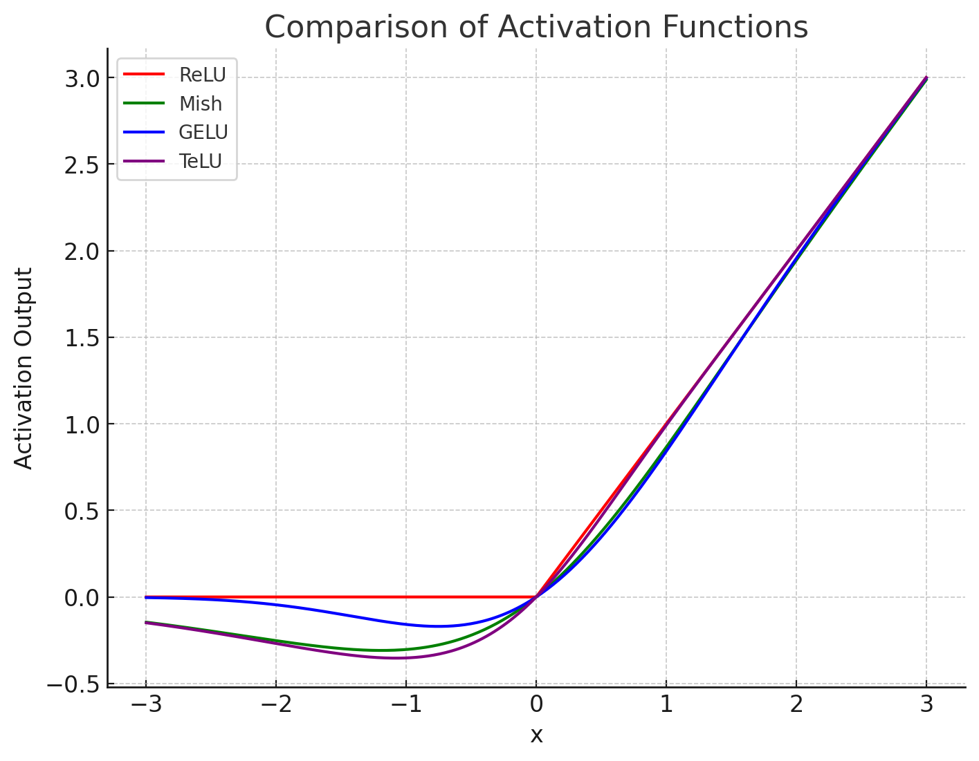
Figure 1: The characteristic of the TeLU activation function along with ReLU, GELU and Mish.

The Hyperbolic Tangent Exponential Linear Unit (TeLU) activation function represents a notable advancement in neural network design, marrying practical performance with theoretical robustness. Mathematically TeLU is represented as follows:

$$f(x)=x{\cdot}tanh(e^{x})$$ (1)

TeLU elegantly integrates the linear characteristics of traditional activation functions with the non-linear benefits of exponential and hyperbolic tangent functions. This fusion ensures that TeLU maintains a balance between facilitating efficient learning and preventing gradient-related issues (credit assignment) commonly encountered in deep neural networks. At the heart of TeLU’s design is the hyperbolic tangent of the exponential function, which intuitively moderates the activation’s output, ensuring it remains within a manageable range. This characteristic is crucial in mitigating the risk of exploding gradients, a common pitfall in deep network training. Moreover, unlike some of its predecessors, TeLU offers a smooth transition across the origin, which enhances the gradient flow through the network. This smoothness is particularly beneficial in deep learning models, as it contributes to more stable and consistent learning dynamics. This can be visualized in Figure 1, which shows the continuity of the TeLU and also that it saturates at a lower rate compared to other SoTA functions.

Furthermore, TeLU’s formulation brings theoretical benefits, particularly in the Fisher Information Matrix (FIM) context. This aspect of TeLU underpins a smoother optimization landscape, a property that directly correlates with enhanced training stability and convergence. It is evident from figure 2, where the second derivative of Mish saturates, whereas GELU and TeLU are much more stable. One important thing to note is that TeLU, for large values, comes closer to GELU, which can also validate its empirical performance.

Mathematical Analysis

In this section, we mathematically prove several properties of TeLU, including credit assignment issues, stability, robustness, and convergence.

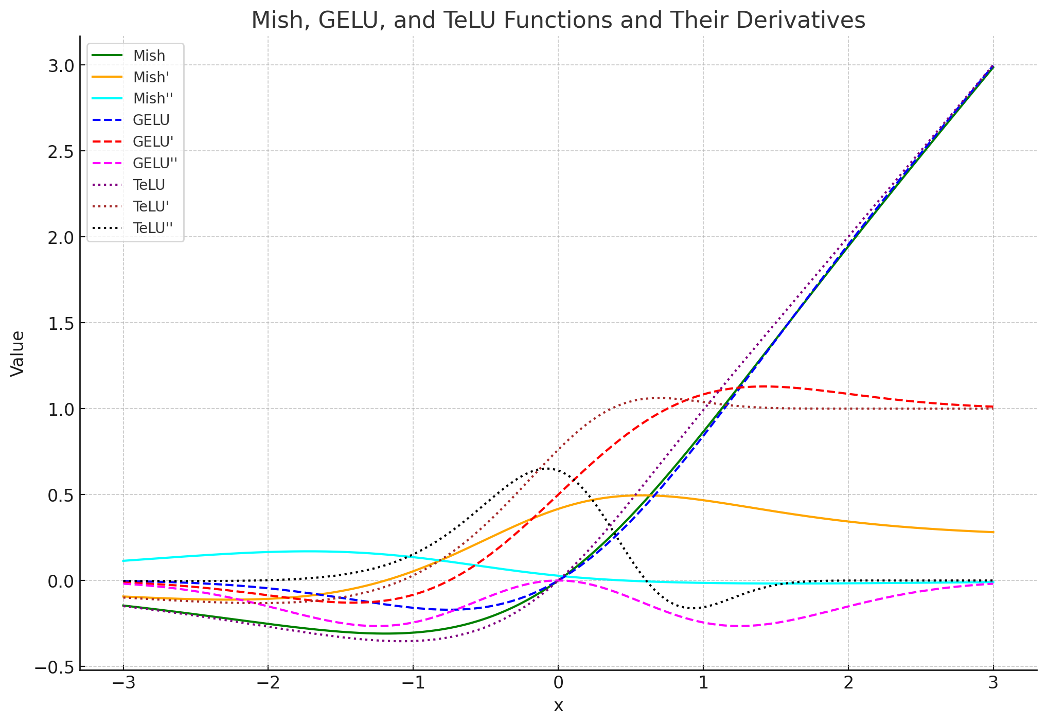
Figure 2: The first and second derivative of proposed TeLU activation compared to derivatives of GELU and Mish

Let $\sigma$ be an activation function given as $y=\sigma(x)$, where x is the input and y is the output. Let $\mathcal{F}(\Theta)$ be the set of parameters using the $\sigma$ non-linearities. Let the function $\mathcal{f}$ be optimized by the objective function $\mathcal{L}(\Theta)$ using standard backpropagation of error, then we show $\sigma$ applied on any function ${f}$ avoids vanishing gradients issues in the neural network.

Theorem 1

If f(x) = $x\cdot\tanh(e^{x})$, then it avoids gradient vanishing problem since $f^{\prime}(x)\neq 0\text{ for all }x\in\mathbb{R}$.

Proof:

The derivative of ${f}(x)$ with respect to $x$ is given by:

$${f}^{\prime}(x)=\frac{d}{dx}\left(x\cdot\tanh(e^{x})\right).$$

Applying the product rule and the chain rule, we find:

$$f^{\prime}(x)=\tanh(e^{x})+x\cdot(1-\tanh^{2}(e^{x}))\cdot e^{x}.$$

We analyze this derivative of above function in two parts:

• $\tanh(e^{x})$ is always non-negative, as for some value of z the $\tanh(z)$ is bounded between -1 and 1 for all $z$ and $e^{x}$ is always positive.

• $1-\tanh^{2}(e^{x})$ is always positive since $|\tanh(z)|<1$ for all $z$, and $e^{x}$ is always positive for all real $x$

Thus, the second term $x\cdot(1-\tanh^{2}(e^{x}))\cdot e^{x}$ is always non-zero unless $x=0$. However, even at $x=0$, the first term $\tanh(e^{x})$ remains non-zero. Therefore, the entire expression for $f^{\prime}(x)$ is non-zero for all $x$.

Hence, we conclude:

$$f^{\prime}(x)\neq 0\text{ for all }x\in\mathbb{R}.$$

$\square$

Next, we show TeLU exhibits the saturating behavior thus under mild assumption, can avoid exploding gradient issues in neural network

Theorem 2

Let $f(x)=x\cdot\tanh(e^{x})$. Then for $x>0$, $f(x)$ exhibits controlled growth, and for $x\leq 0$, $f(x)$ shows saturating behavior. The derivative $f^{\prime}(x)$ remains finite for all $x\in\mathbb{R}$, contributing to the mitigation of exploding gradients.

Proof:

We now analyze the function $f(x)$ and its derivative $f^{\prime}(x)$ in two regions: for $x>0$ and $x\leq 0$.

Controlled Growth for Positive Values:

For $x>0$, the exponential function $e^{x}$ grows rapidly. However, the hyperbolic tangent function $\tanh(z)$ is bounded and saturates, where $\lim_{z\to\infty}\tanh(z)=1$. Therefore, for large positive values of $x$, $f(x)$ grows linearly, as $f(x)\approx x$ due to the saturation of $\tanh(e^{x})$ towards 1. This linear growth prevents the function from exhibiting exponential growth with a bound, thus mitigating the risk of exploding gradients.

Saturating Behavior for Negative Values:

For $x\leq 0$, as $x\to-\infty$, the term $e^{x}$ approaches 0, causing $\tanh(e^{x})$ to also approach 0. Consequently, $f(x)$ approaches 0, showing a saturating behavior as $x$ becomes large in the negative direction.

Now Lets consider the derivative $f^{\prime}(x)$:

$$f^{\prime}(x)=\tanh(e^{x})+x\cdot(1-\tanh^{2}(e^{x}))\cdot e^{x},$$

we observe that for positive $x$, $f^{\prime}(x)$ remains finite due to the saturation of $\tanh(e^{x})$ and the controlled growth of $x\cdot(1-\tanh^{2}(e^{x}))\cdot e^{x}$. For negative $x$, the derivative tends towards 0, reflecting the saturating behavior of $f(x)$.

Hence, we conclude that $f(x)=x\cdot\tanh(e^{x})$ exhibits controlled growth for positive values and saturating behavior for negative values, which contributes to avoiding exploding gradients for positive values of $x$ within a bound. $\square$

Next, we show that TeLU has an implicit regularization, thus avoiding overfitting, exhibits stable behavior, zero-mean activation [22] and converges faster.

Theorem 3

Let $f(x)=x\cdot\tanh(e^{x})$. If $x$ is a random variable following a symmetric probability distribution about zero, then the expected value (mean) of $f(x)$ is approximately zero, and f(x) provides efficient gradient flow and implicit regularization.

$$\lim_{a\to\infty}\frac{1}{2a}\int_{-a}^{a}f(x)\,dx=0$$

Proof:

$$1.\quad \text{Let }f(x)=x\cdot\tanh(e^{x}).$$

$$2.\quad \text{Near Zero: }\lim_{x\to 0}f(x)=\lim_{x\to 0}x\cdot\tanh(e^{x})=0.$$

$$3.\quad \text{Away from Zero: }\lim_{x\to\pm\infty}f(x)=\pm\infty.$$

$$4.\quad \text{Consider }I(a)=\int_{-a}^{a}f(x)\,dx.$$

$$5.\quad \text{For large }a,\text{ the positive and negative values of }f(x)\text{ over }[-a,a]\text{ counterbalance each other.}$$

$$6.\quad \text{Therefore, }\lim_{a\to\infty}\frac{1}{2a}I(a)=\lim_{a\to\infty}\frac{1}{2a}\int_{-a}^{a}f(x)\,dx=0.$$

Thus the function $f(x)=x\cdot\tanh(e^{x})$ has an asymptotic mean-shifting property towards zero. $\square$

In the appendix 9, we show mathematically that the mean of the activation for ReLU doesn’t approach zero. Next, we prove the network’s stability and explain why TeLU has the lowest variance among competing activation functions.

Theorem 4

The function $f(x)=x\cdot\tanh(e^{x})$ exhibits stable behavior for any neural network.

Proof:

Bounded Output: The hyperbolic tangent function $\tanh(z)$ has outputs bounded between -1 and 1. Therefore, for any real number $x$, the product $x\cdot\tanh(e^{x})$ will not grow unbounded, contributing to stability. Mathematically, this can be expressed as:

$$-|x|\leq f(x)\leq|x|$$

2. Non-zero Gradient: The derivative of $f(x)$, given by

$$f^{\prime}(x)=\tanh(e^{x})+x\cdot(1-\tanh^{2}(e^{x}))\cdot e^{x}$$

is always non-zero for all real numbers $x$. This ensures that the gradients do not vanish during backpropagation, which is crucial for stable learning in deep networks.

3. Controlled Growth for Positive $x$: For positive $x$, the function grows linearly since $\tanh(e^{x})$ approaches 1. This linear growth is more stable than exponential growth, which could lead to exploding gradients.

4. Saturating Behavior for Negative $x$: For negative $x$, as $x$ becomes large in the negative direction, $f(x)$ approaches 0. This saturation helps prevent the function from contributing to exploding gradients during training.

Therefore, due to its bounded output, non-zero gradient, controlled growth for positive values, and saturating behavior for negative values, the function $f(x)=x\cdot\tanh(e^{x})$ is shown to be stable in the context of neural network activations. $\square$

Next, we show TeLU is more robust to small noise and perturbations compared to ReLU, which is an important property to design adversarial-resistant neural network

Theorem 5

The function $f(x)=x\cdot\tanh(e^{x})$ is more robust compared to Relu ($g(x)=max(0,x)$) and robust against small perturbations or noise in the input.

Proof:

We analyze the derivative of $f(x)$ to show robustness to small perturbations. The derivative gives the rate of change of the function with respect to changes in the input. A small derivative magnitude indicates robustness to small changes or noise in the input. The derivative of g(x) = Relu is represented as follows:

$$\text{g}^{\prime}(x)=\begin{cases}0&\text{if }x<0\\ 1&\text{if }x>0\\ \text{undefined}&\text{if }x=0\end{cases}$$

This derivative shows that for $x>0$, the function is sensitive to changes, as even small positive changes in $x$ will result in a change in output. The function is insensitive to changes for $x<0$, as the output remains zero. The derivative is undefined at $x=0$, indicating a discontinuity, which can be problematic for stability.

The derivative of $f(x)=TeLU$ is given by:

$$f^{\prime}(x)=\tanh(e^{x})+x\cdot(1-\tanh^{2}(e^{x}))\cdot e^{x}$$

Consider the behavior of $f^{\prime}(x)$ for different ranges of $x$:

For large negative $x$: As $x$ becomes very negative, $e^{x}$ approaches 0, making $\tanh(e^{x})$ and its derivative small. Thus, $f^{\prime}(x)$ becomes small, indicating that $f(x)$ is not highly sensitive to small changes in $x$.

For small $x$ around 0: Here, $\tanh(e^{x})$ is approximately equal to $e^{x}$, which is close to 1 for small $x$. The term $x\cdot(1-\tanh^{2}(e^{x}))\cdot e^{x}$ is also small. Hence, $f^{\prime}(x)$ remains moderate, suggesting that $f(x)$ does not change drastically for small perturbations around 0.

For large positive $x$: Although $e^{x}$ grows, the term $\tanh(e^{x})$ approaches 1, limiting the growth of $f(x)$. The term $x\cdot(1-\tanh^{2}(e^{x}))\cdot e^{x}$ becomes small as $x$ increases, due to the saturation of $\tanh(e^{x})$. Thus, $f^{\prime}(x)$ remains bounded.

Since $f^{\prime}(x)$ does not exhibit large values across the range of $x$, it indicates that $f(x)$ does not change disproportionately for small changes in $x$, thereby demonstrating robustness to small perturbations or noise. $\square$

Next, we show a strong property which shows TeLU is Lipschitz continuous, which is important to uniform continuity of the function

Theorem 6

The function $f:\mathbb{R}\to\mathbb{R}$, defined by $f(x)=x\cdot\tanh(e^{x})$, is Lipschitz continuous on the real line $\mathbb{R}$.

Proof:

To demonstrate that $f$ is Lipschitz continuous, we seek a constant $L$ such that for all $x,y\in\mathbb{R}$, the inequality

$$|f(x)-f(y)|\leq L|x-y|$$

is satisfied. A sufficient condition for this is that the derivative of $f$, $f^{\prime}(x)$, is bounded on $\mathbb{R}$.

The derivative of $f$ is given by

$$f^{\prime}(x)=\tanh(e^{x})+x\cdot\frac{e^{x}}{\cosh^{2}(e^{x})}$$

We analyze the boundedness of $f^{\prime}(x)$ in two parts:

1. The function $\tanh(e^{x})$ is bounded on $\mathbb{R}$ as $\tanh$ outputs values in $(-1,1)$.

2. For the term $x\cdot\frac{e^{x}}{\cosh^{2}(e^{x})}$, we consider its behavior as $x$ approaches infinity and negative infinity:

$$\lim_{x\to\infty}\left|x\cdot\frac{e^{x}}{\cosh^{2}(e^{x})}\right|=1$$

$$\lim_{x\to-\infty}\left|x\cdot\frac{e^{x}}{\cosh^{2}(e^{x})}\right|=0$$

Since both limits are finite, the term $x\cdot\frac{e^{x}}{\cosh^{2}(e^{x})}$ is bounded on $\mathbb{R}$.

Combining these findings, we conclude that $|f^{\prime}(x)|$ is bounded on $\mathbb{R}$. The maximum value of $|f^{\prime}(x)|$ is $1$, therefore we can take $L=1$ as the Lipschitz constant.

Hence, $f(x)=x\cdot\tanh(e^{x})$ is Lipschitz continuous with a Lipschitz constant $L=1$. $\square$

Next, we show that TeLU has a smoother loss landscape, which leads to faster convergence.

Theorem 7

Given a neural network $\mathcal{N}$ with activation function $f(x)=x\cdot\tanh(e^{x})$, parameters $\theta$, and a differentiable loss function $\mathcal{L}(\theta)$, the Fisher Information Matrix $I(\theta)$ defined as

$$I(\theta)=\mathbb{E}_{(x,y)\sim\mathcal{D}}\left[\nabla_{\theta}\log p(y|x;\theta)\nabla_{\theta}\log p(y|x;\theta)^{\top}\right]$$

leads to a smoother optimization landscape during training of $\mathcal{N}$.

Proof Sketch: Based on prior results, we show the smoothness of TeLU and its derivative and how it leads to better Fisher information estimates [5]. The detailed proof can be found in the appendix B

Finally we show with some mild assumption (Polyak-Łojasiewicz (PL) condition [21]) the global convergence of network trained using TeLU

Theorem 8

Let $\mathcal{N}$ be a neural network employing the activation function $f(x)=x\cdot\tanh(e^{x})$ in its architecture. Assume the network parameters are denoted by $\theta$ and the network is trained using a differentiable loss function $\mathcal{L}(\theta)$. If $\mathcal{L}(\theta)$ satisfies the Polyak-Łojasiewicz (PL) condition, then the gradient descent optimization on $\mathcal{N}$ converges to a global minimum, significantly influenced by the properties of $f(x)$ and it’s derivative $f^{\prime}(x)$.

Proof Sketch: We adapt this based on prior constructions, showing TeLU converges faster and has a smooth optimization curve and proving using PL condition that the network will converge to global optima. The detailed proof is shown in appendix B

Next, we empirically validate the effectiveness of the proposed TeLU activation function

3 Experiments using TeLU

This section presents a detailed assessment of the TeLU activation function implemented within deep neural architectures, specifically Squeezenet [12] and Resnet-18/32/50 [8]. Our evaluation focuses on the stability and performance of TeLU across diverse optimization techniques, including Stochastic Gradient Descent (SGD) [24], SGD with Momentum [16], AdamW [17]. and RMSprop [7]. We benchmark TeLU’s effectiveness by comparing it with a range of established activation functions: (i) ReLU [6], (ii) GELU [9], (iii) Mish [19], (iv) SiLU [23], (v) Smish [28], and (vi) Logish [29].

Datasets

We utilized three benchmark datasets to evaluate our proposed model: CIFAR-10, CIFAR-100 [13], and TinyImageNet [14]. Each of these datasets is crucial for benchmarking the performance of image classification algorithms, especially Convolutional Neural Networks (CNNs).

CIFAR-10: This dataset comprises $60,000$ color images of dimensions $32\times 32$ pixels, evenly distributed across $10$ distinct classes. The dataset is partitioned into a training set of $50,000$ images and a test set of $10,000$ images. We split the dataset into $45,000$ images for training, $5,000$ images for validation, and $10,000$ for testing.

CIFAR-100: Similar in size to CIFAR-10, CIFAR-100 contains $60,000$ color images of $32\times 32$ pixels. However, it is differentiated by its finer categorization into $100$ classes, with each class containing $600$ images. We split the dataset into $45,000$ images for training, $5,000$ images for validation, and $10,000$ for testing.

TinyImageNet: As a subset of the larger ImageNet dataset, TinyImageNet includes $110,000$ images resized to $64\times 64$ pixels. It spans $200$ classes, with each class contributing $500$ training images, $50$ validation images, and $50$ test images. We utilize the original training set of $100,000$ images and validation set of $10,000$ images, as no testing set is publicly available for TinyImageNet.

Experimental Setup

In our experimental framework, the activation function was the sole independent variable across all models, facilitating a focused analysis of its impact on model performance. These activation functions include TeLU, ReLU, GELU, Mish, SiLU, Smish, and Logish. We employed a comprehensive grid search methodology to meticulously optimize key hyperparameters – learning rate, learning rate decay (gamma), learning rate decay step size, and weight decay – thereby ensuring maximal accuracy on the validation subsets for a broad spectrum of activation function configurations. These hyperparameters were fine-tuned for each experimental setup, with their optimal values enumerated in the appendix for reference. We maintained a consistent batch size of $128$ across all trials to ensure uniformity in training conditions. For CIFAR-10 and CIFAR-100 experiments, the learning rate was decayed at epochs 60, 120, and 160. For TinyImageNet experiments, the learning rate steps occurred at 60, 100, 140, and 170. The optimal initial learning rate, learning rate decay gamma coefficient, and weight decay hyperparameters were identified based on their performance enhancement on the validation dataset. These tuned hyperparameters are detailed in supplementary tables: 4, 5, 6, 7, 24, 25, 26, 27, 44. Each experiment was conducted over $200$ epochs per model, and these were replicated across 5 distinct trials to guarantee statistical robustness. Our experimental matrix was extensive, encompassing a diverse array of datasets (CIFAR-10, CIFAR-100, and TinyImageNet), neural network architectures (SqueezeNet, ResNet18, ResNet34, and ResNet50), and optimization algorithms (SGD, SGD with Momentum, AdamW, and RMSprop). It is noteworthy that for experiments involving the TinyImageNet dataset, we exclusively utilized the ResNet34 architecture due to computational limits.

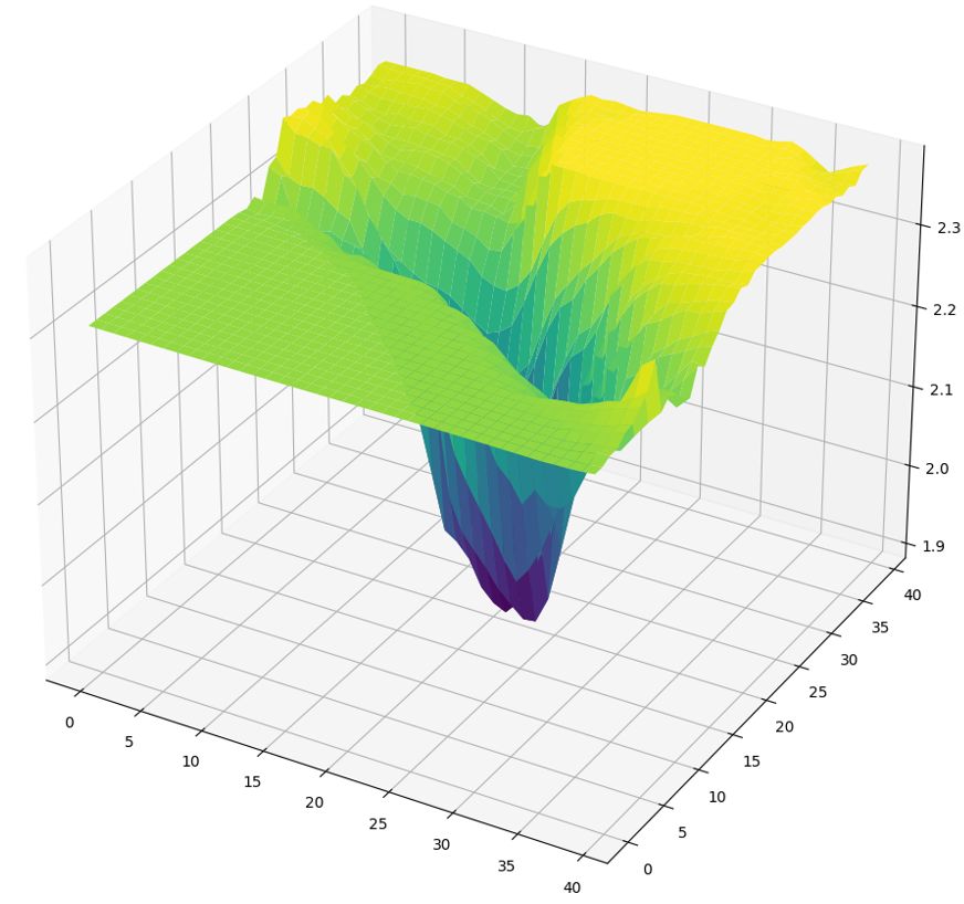
Figure 3: ReLU Loss Landscape

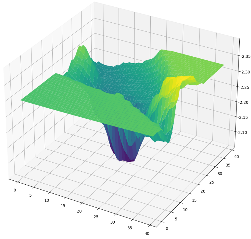
Figure 4: TeLU Loss Landscape

CIFAR-10 Experiments

The primary objective of these experiments was to rigorously evaluate the generalization efficacy of various activation functions within the context of complex, natural image datasets. Table 1 presents a comparative analysis of different activation functions applied to the Squeezenet architecture on the CIFAR-10 dataset. The results delineated in Table 1 clearly demonstrate that the TeLU activation function consistently surpasses its counterparts in most scenarios, not only in terms of performance but also by exhibiting a notably lower variance.

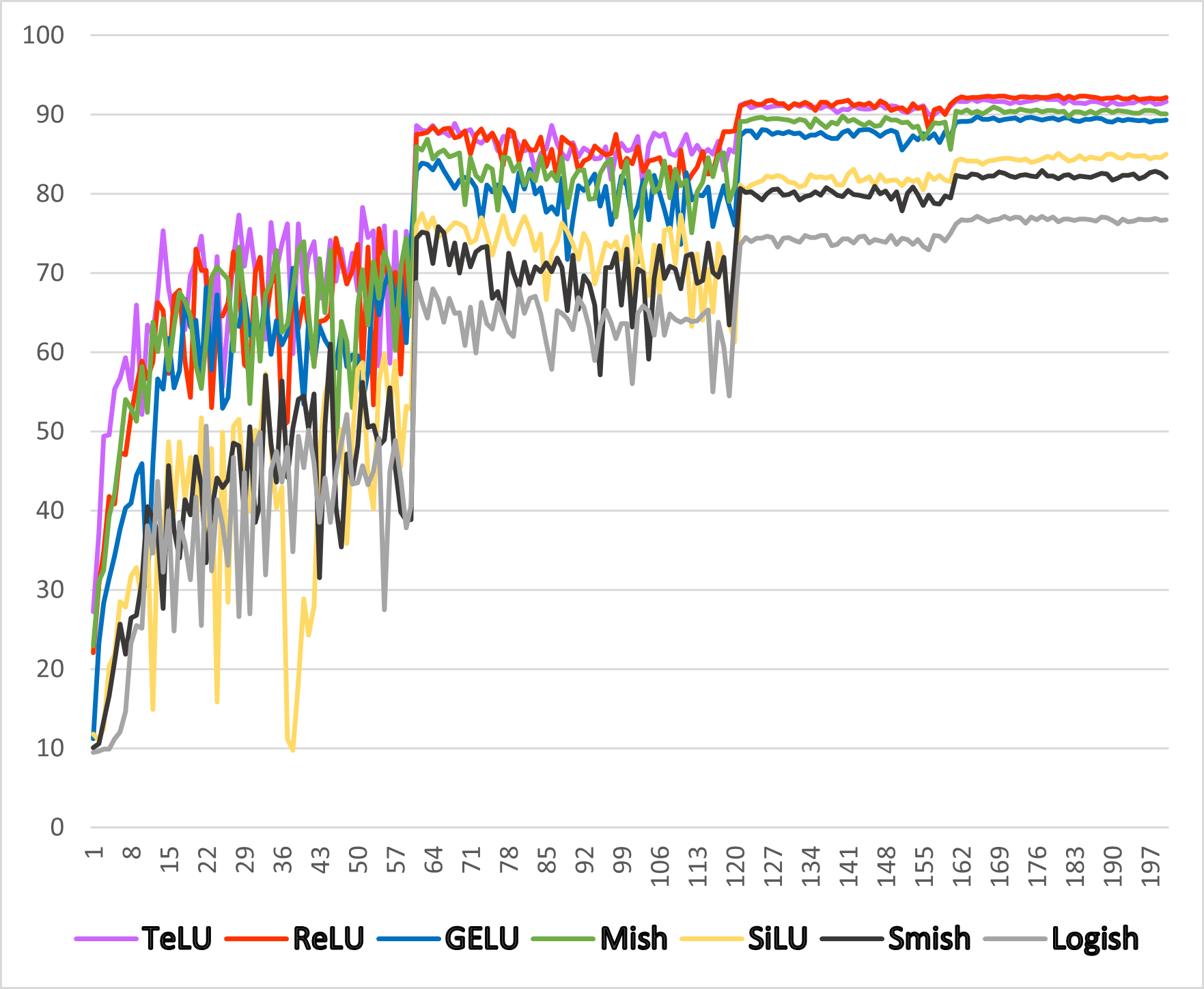
Figure 5: Validation performance comparison of 7 activation functions per epoch on CIFAR-10 using SqueezeNet-SGD

For instance, a comparative case involving Logish highlights its underperformance, particularly when trained using SGD, where it exhibits a significant variance of 29. It’s crucial to acknowledge that while each network was meticulously optimized for each optimizer, Logish achieved a peak accuracy of 90% on one seed but exhibited marked performance degradation on others. Furthermore, a close examination reveals that ReLU, albeit being the second most effective activation function in our study, experiences a performance decline of 3.25% when transitioning from SGD to RMSProp. In stark contrast, TeLU maintains robustness across optimizers, evidenced by the smallest average performance drop of merely 1.84%. This is also evident in Figure 5 and 6 we show per epoch validation curve for each activation function for a trial. This underscores TeLU’s superior adaptability and stability across different optimization environments. In figure 3 and 4, we plot the 3D loss landscape surface for both ReLU and TeLU, respectively, thus validating our theoretical findings. We observe a similar trend for the other 3 architectures; we report the results in appendix C.

Table 1: CIFAR-10 SqueezeNet Test Accuracy Summary

Name	SGD	Momentum	AdamW	RMSprop
TeLU	91.40$\pm$ 0.11	90.96$\pm$0.29	90.08$\pm$0.77	89.86$\pm$0.28
ReLU	91.84$\pm$0.33	90.77$\pm$0.16	89.01$\pm$0.45	88.59$\pm$0.14
GELU	88.42$\pm$0.28	89.33$\pm$0.24	89.63$\pm$0.70	80.68$\pm$1.2
Mish	89.87$\pm$0.21	90.04$\pm$0.25	89.02$\pm$87	87.39$\pm$0.17
SiLU	78.61$\pm$6.3	84.10$\pm$1.1	86.70$\pm$1.9	66.00$\pm$1.3
Smish	77.28$\pm$3.0	68.60$\pm$2.2	41.71$\pm$17	66.91$\pm$2.3
Logish	61.44$\pm$29	66.10$\pm$3.6	42.72$\pm$16	43.20$\pm$19

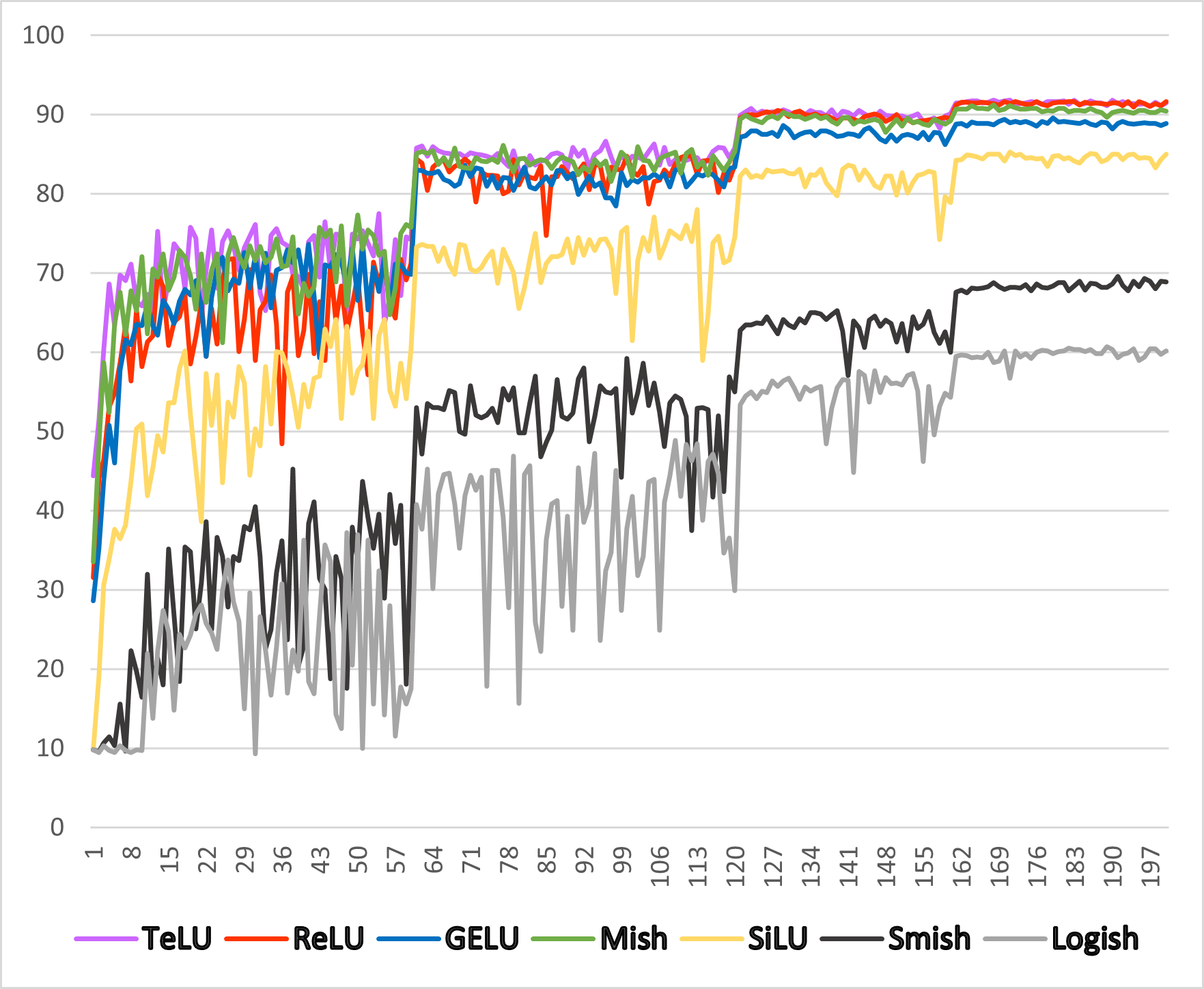
Figure 6: Validation performance comparison of 7 activation functions per epoch on CIFAR-10 using SqueezeNet Momentum

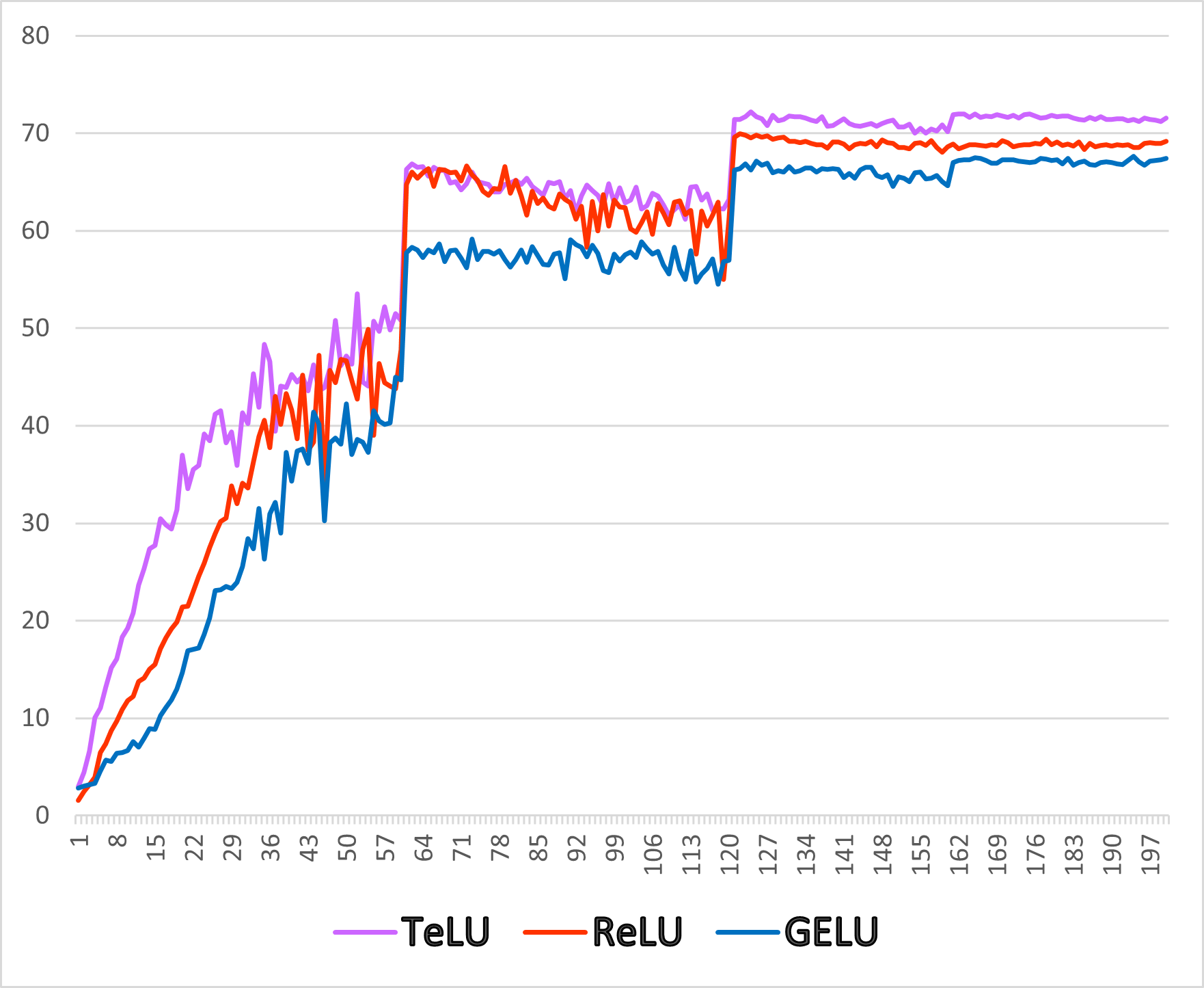
Figure 7: Validation performance comparison of TeLU, ReLU and GELU per epoch on CIFAR-100 using SqueezeNet SGD

In this section, we extend our analysis to the CIFAR-100 benchmark, focusing on evaluating the robustness of our TeLU (Hyperbolic Tangent Exponential Linear Unit) activated model in extracting intricate features and its resilience against overfitting to specific class attributes. The intrinsic regularization properties of TeLU contribute to its reduced overfitting tendencies when compared to ReLU, which, in our experimental setup, displayed comparable performance to TeLU. Our prior investigations revealed a significant similarity in the hyperparameter landscape for TeLU, ReLU, and GELU, in contrast to the other four evaluated activation functions. This similarity facilitates a more streamlined and efficient hyperparameter optimization process. Building on the preliminary findings, which indicated a propensity for larger variance in other activation functions, we confined our subsequent experiments to the top-performing trio of activation functions (TeLU, ReLU, and GELU). This phase involved a comprehensive evaluation across four different architectural frameworks, employing four distinct optimization algorithms. The comparative results are meticulously detailed in Table 2, where TeLU’s consistent top-tier performance across various optimizers is underscored alongside its characteristic lower variance profile.

Table 2: CIFAR-100 SqueezeNet Test Accuracy Summary

Name	SGD	Momentum	AdamW	RMSprop
TeLU	71.47$\pm$0.08	70.53$\pm$0.25	69.64$\pm$0.07	68.83$\pm$0.33
ReLU	69.52$\pm$0.43	65.05$\pm$0.51	66.31$\pm$0.48	67.99$\pm$0.21
GELU	67.09$\pm$0.36	66.26$\pm$29	66.50$\pm$0.44	65.19$\pm$0.25

CIFAR-100 Experiments

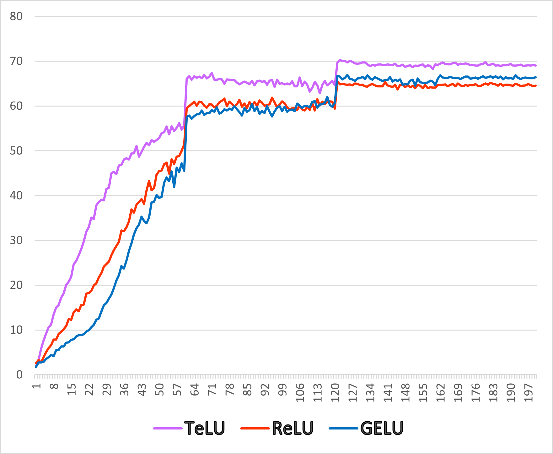
Figure 8: Validation performance comparison of TeLU, ReLU and GELU per epoch on CIFAR-100 using Momentum

The empirical outcomes are further elucidated through Figures 7 and 8, which depict the validation performance of models employing Squeezenet architecture and trained using SGD and Momentum optimizers, respectively. These visual representations clearly demonstrate TeLU’s superior convergence rate relative to ReLU and GELU, ultimately leading to more optimal solutions. This enhanced convergence efficiency of TeLU is particularly notable in the context of complex datasets like CIFAR-100, reinforcing its potential as a highly effective activation function in advanced neural network applications. In the appendixC, we report performance for the remaining 3 architectures, where a similar trend was observed.

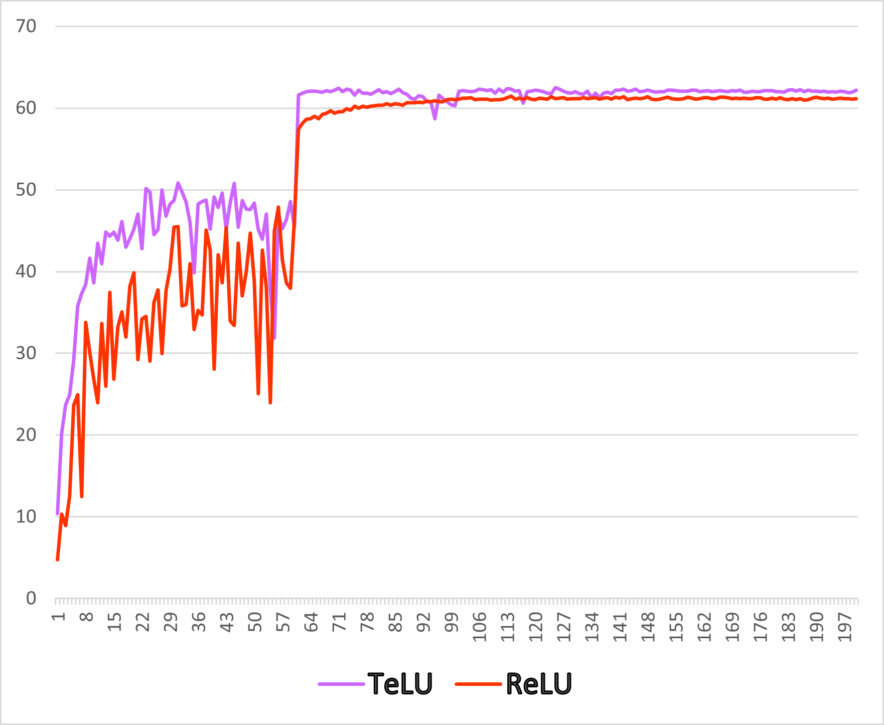
Figure 9: Validation performance comparison of TeLU, ReLU per epoch on TinyImagenet using Resnet-34 SGD.

TinyImageNet200 Experiments

In this detailed analysis, we probe the hierarchical representation learning capabilities of the TeLU (Hyperbolic Tangent Exponential Linear Unit) activation function within high-dimensional, complex imagery contexts, employing the Resnet-34 architecture—a model noted for its depth and complexity. Given that our preceding analysis positioned TeLU and ReLU as the leading activation functions, we conducted a focused evaluation using the TinyImagenet benchmark to compare their performance intricacies. The results, systematically tabulated in Table 3, reveal a consistent outperformance by TeLU over ReLU. A particularly intriguing observation is the marked inconsistency of ReLU under Momentum-based training. We noted that while ReLU achieved an accuracy peak of nearly 64% for one specific seed, its performance plummeted to below 20% for other seeds, resulting in an extraordinarily high variance of 34%. This variability is a critical indicator of ReLU’s instability under certain training conditions. Figure 10 presents the maximum, mean, and minimum performance metrics for both TeLU and ReLU to visually encapsulate and further scrutinize this instability. This graphical representation provides a clear and comprehensive view of the performance disparities between the two activation functions. Additionally, Figure 9 focuses on the models trained using the Stochastic Gradient Descent (SGD) optimizer, where ReLU demonstrates a more stable behavior. Despite this stability, it is noteworthy that TeLU exhibits a significantly accelerated convergence rate even in this scenario compared to ReLU, indicating its efficiency in navigating toward optimal solutions more rapidly. This aspect is particularly critical in deep learning models where time-to-convergence is vital in evaluating the effectiveness of activation functions.

Table 3: TinyImageNet ResNet34 Test Accuracy Summary.

Name	SGD	Momentum	AdamW	RMSprop
TeLU	62.34$\pm$0.17	62.09$\pm$0.22	54.04$\pm$0.82	58.48$\pm$0.03
ReLU	61.16$\pm$0.31	38.37$\pm$34	54.88$\pm$0.72	58.33$\pm$0.27

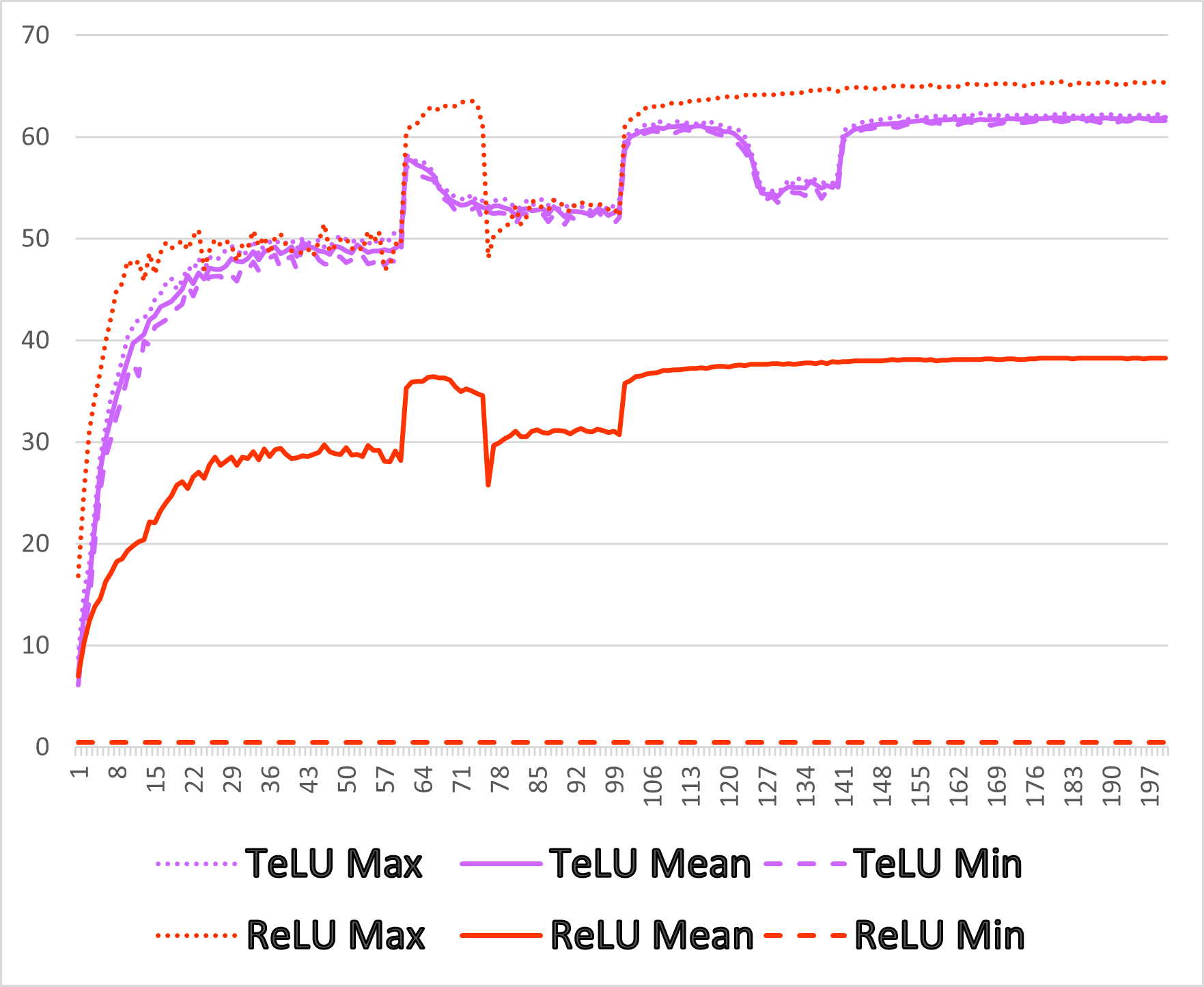
Figure 10: Validation accuracy per epoch on TinyImageNet using ResNet34-Momentum. TeLU and ReLU Validation curves are shown for best, mean, and minimum scenarios across 5 trials.

4 Conclusion

In this work, we have successfully introduced the TeLU, a novel activation function designed to catalyze stable, efficient, and robust learning in deep neural networks. TeLU is Lipschitz continuous and saturates towards large negative value. For symmetric probability distribution, TeLU shifts the activation mean towards zero, which aligns gradients more closely with unit natural gradients, thereby accelerating convergence and introducing stability. Furthermore, TeLU’s controlled growth for positive inputs and its saturating behavior for negative values underscore its robustness and stability – vital attributes for reliable neural network performance. Empirical evidence strongly supports TeLU’s superiority. Across three major vision benchmarks, TeLU consistently outshines other activation functions. It exhibits remarkable stability across various experimental conditions, starkly contrasting the often unstable behaviors observed with ReLU and GELU under similar circumstances. TeLU’s consistency across different optimization strategies is particularly noteworthy, reaching near-uniform conclusions and exhibiting minimal variance in performance.

5 Impact Statement

In this work, we have introduced a novel activation function, poised to improve neural network training with properties such as theoretical stability, rapid convergence, and enhanced robustness. This innovative approach is a positive step towards an efficient neural network, which promises a positive direction in significantly reducing energy consumption, a vital step towards more sustainable and environmentally friendly AI technologies. By focusing on creating more efficient models, we are paving the way for a future where advanced deep learning can be both high-performing and energy-conscious. While our contribution marks a significant advancement in technical aspects of neural network design, we acknowledge that it does not directly address the broader social, ethical, fairness, and bias challenges inherent in deep learning architectures. These issues require a holistic approach, combining technical innovation with rigorous ethical standards and inclusive practices to ensure AI is fair and beneficial for all.

Appendix A Robustness comparison of TeLU with other activations

We compare the robustness of Mish, GELU, ELU [3], and $f(x)=x\cdot\tanh(e^{x})$ functions by examining and comparing their derivatives.

1. Mish Function:

$$\text{Mish}(x)=x\cdot\tanh(\ln(1+e^{x}))$$

The derivative is complex, involving the derivative of tanh and the exponential function.

2. GELU Function:

$$\text{GELU}(x)\approx 0.5x\left(1+\tanh\left[\sqrt{2/\pi}\left(x+0.044715x^{3}\right)\right]\right)$$

The derivative involves both tanh and polynomial components.

3. ELU Function:

$$\text{ELU}(x)=\begin{cases}x&\text{if }x>0\\ \alpha(e^{x}-1)&\text{if }x\leq 0\end{cases}$$

$$\text{ELU}^{\prime}(x)=\begin{cases}1&\text{if }x>0\\ \alpha e^{x}&\text{if }x\leq 0\end{cases}$$

4. $f(x)=x\cdot\tanh(e^{x})$ Function:

$$f(x)=x\cdot\tanh(e^{x})$$

$$f^{\prime}(x)=\tanh(e^{x})+x\cdot(1-\tanh^{2}(e^{x}))\cdot e^{x}$$

The robustness of these functions to small input perturbations can be inferred from the behavior of their derivatives. A large derivative in magnitude or varies rapidly with respect to $x$ indicates less robustness to small changes in input. In contrast, a derivative that remains bounded and changes smoothly suggests greater robustness.

Based on this criterion, we can qualitatively rank the robustness of these functions, which ranks TeLU first, followed by GELU, ELU, and then Mish.

Appendix B Convergence Guarantee of TeLU

First, we show ReLU doesn’t have mean shifting property and doesn’t exhibit a regularization effect

Theorem 9

The Rectified Linear Unit (ReLU) function, defined as $\text{ReLU}(x)=\max(0,x)$, does not exhibit mean-shifting capability over symmetric intervals $[-a,a]$ around zero

Proof:

1. $\text{ReLU}(x)=\max(0,x)$. This implies $\text{ReLU}(x)=0$ for $x\leq 0$ and $\text{ReLU}(x)=x$ for $x>0$.

2. Consider $I(a)=\int_{-a}^{a}\text{ReLU}(x)\,dx$.

3. Splitting the integral:

   $$I(a)=\int_{-a}^{0}\text{ReLU}(x)\,dx+\int_{0}^{a}\text{ReLU}(x)\,dx$$

4. Evaluating the integrals:

   $$I(a)=0+\int_{0}^{a}x\,dx=0+\frac{a^{2}}{2}$$

5. Average value over $[-a,a]$:

   $$\frac{1}{2a}I(a)=\frac{a}{4}$$

6. As $a$ increases, the average value increases, not approaching zero.

This concludes the proof $\square$

Next, we show that TeLU ($f(x)$) and its derivative ($f^{\prime}(x)$) are both continuous, and that this condition is true even based on the Intermediate Value Theorem (IVT) [1] and the Mean Value Theorem (MVT) [2].

Theorem 10

Let $f(x)=x\cdot\tanh(e^{x})$ be defined for all $x\in\mathbb{R}$. Then:

1. The function $f(x)$ and its derivative $f^{\prime}(x)$ are continuous for all $x\in\mathbb{R}$.

2. The function $f(x)$ satisfies the Intermediate Value Theorem (IVT) on any interval $[a,b]\subset\mathbb{R}$.

3. The function $f(x)$ satisfies the Mean Value Theorem (MVT) on any interval $[a,b]\subset\mathbb{R}$, where $a\neq b$.

Proof:

Continuity of $f(x)$ and $f^{\prime}(x)$

• $f(x)=x\cdot\tanh(e^{x})$ is continuous as both $x$ and $\tanh(e^{x})$ are continuous.

• The derivative $f^{\prime}(x)=\tanh(e^{x})+x\cdot sech^{2}(e^{x})\cdot e^{x}$ is continuous since $\tanh(e^{x})$, $sech^{2}(e^{x})$, and $e^{x}$ are continuous.

Application of the IVT

The Intermediate Value Theorem [1] states that if a function is continuous on a closed interval, then it takes on every value between its values at the endpoints of the interval.

• For $f(x)$ on any interval $[a,b]$, if $d$ is a value between $f(a)$ and $f(b)$, there exists a $c\in[a,b]$ such that $f(c)=d$.

• This is because $f(x)$ is continuous on $[a,b]$.

• Similarly, since $f^{\prime}(x)$ is continuous on any interval $[a,b]$, by IVT, for any value $e$ between $f^{\prime}(a)$ and $f^{\prime}(b)$, there exists a $c\in[a,b]$ such that $f^{\prime}(c)=e$.

Application of the MVT

The Mean Value Theorem [2] states that if a function is continuous on a closed interval and differentiable on the open interval, then there exists at least one point in the open interval where the derivative equals the average rate of change over the closed interval.

• Since $f(x)$ is continuous on $[a,b]$ and $f^{\prime}(x)$ is continuous on $(a,b)$, by MVT, there exists at least one $c\in(a,b)$ such that $f^{\prime}(c)=\frac{f(b)-f(a)}{b-a}$.

The function $f(x)=x\cdot\tanh(e^{x})$ and its derivative are continuous, and $f(x)$ and $f^{\prime}(x)$ satisfies both the IVT and MVT on any interval in $\mathbb{R}$.

This concludes the proof $\square$

Next we provided detailed proof for Theorem 7 discussed in main paper

Proof:

Continuity and Differentiability of $f(x)$

The activation function $f(x)=x\cdot\tanh(e^{x})$ and its derivative are analyzed:

$$f(x) =x\cdot\tanh(e^{x}),$$

$$\text{where }\tanh(u) =\frac{e^{2u}-1}{e^{2u}+1}.$$

$$\text{Thus, }f^{\prime}(x) =\frac{d}{dx}(x\cdot\tanh(e^{x}))$$

$$=\tanh(e^{x})+x\cdot\frac{d}{dx}\tanh(e^{x})$$

$$=\tanh(e^{x})+x\cdot e^{x}\cdot(1-\tanh^{2}(e^{x})).$$

Since $\tanh(u)$ and $e^{x}$ are continuously differentiable, $f(x)$ and $f^{\prime}(x)$ are also continuously differentiable.

Impact on Fisher Information Matrix

Applying the chain rule to compute the gradient of the log-likelihood:

$$\nabla_{\theta}\log p(y|x;\theta) =\frac{\partial\log p(y|x;\theta)}{\partial\mathcal{N}}\cdot\frac{\partial\mathcal{N}}{\partial\theta},$$

$$=\text{Gradient of the output w.r.t. the network's parameters}.$$

The gradient involves terms from $f^{\prime}(x)$ due to the activation function in each layer:

$$f^{\prime}(x) =\tanh(e^{x})+x\cdot e^{x}\cdot(1-\tanh^{2}(e^{x})).$$

Thus, $I(\theta)$ becomes a matrix of expectations of outer products of these gradients:

$$I(\theta) =\mathbb{E}_{(x,y)\sim\mathcal{D}}\left[\nabla_{\theta}\log p(y|x;\theta)\nabla_{\theta}\log p(y|x;\theta)^{\top}\right].$$

The smoothness of $f^{\prime}(x)$ translates to a smoother $I(\theta)$.

Smoother Optimization Landscape

In gradient descent, parameter updates are governed by:

$$\theta^{(t+1)} =\theta^{(t)}-\eta\cdot\nabla_{\theta}\mathcal{L}(\theta^{(t)}),$$

where $\eta$ is the learning rate. The gradient of the loss function $\nabla_{\theta}\mathcal{L}(\theta)$ is influenced by $I(\theta)$. A smoother $I(\theta)$ results in more stable and consistent gradient updates, avoiding erratic steps often observed in rougher optimization landscapes. This leads to enhanced stability in finding the minima of $\mathcal{L}(\theta)$.

Hence, we can show, that the continuously differentiable nature of $f(x)=x\cdot\tanh(e^{x})$ and its derivative ensures that the Fisher Information Matrix $I(\theta)$ in the neural network $\mathcal{N}$ promotes a smoother optimization landscape, facilitating more effective training dynamics.

$\square$

Based on the properties of TeLU, shown in Theorem 7, we can prove the global convergence of the function under certain conditions.

Now we provided detailed proof for Theorem 8 discussed in main paper

Proof:

Smoothness and Boundedness of $f(x)$ and $f^{\prime}(x)$:

The function $f(x)=x\cdot\tanh(e^{x})$ is continuously differentiable. Its derivative, given by

$$f^{\prime}(x)=\tanh(e^{x})+x\cdot e^{x}\cdot(1-\tanh^{2}(e^{x})),$$

is also continuously differentiable and bounded due to the inherent properties of the $\tanh$ function and the exponential function. These properties ensure smooth and well-conditioned gradient computations throughout the optimization process.

Influence on Gradient Descent under PL Condition:

Given the PL condition, for a global minimum $\theta^{*}$, there exists $\mu>0$ such that

$$2\mu(\mathcal{L}(\theta)-\mathcal{L}(\theta^{*}))\leq\|\nabla_{\theta}\mathcal{L}(\theta)\|^{2}\text{ for all }\theta.$$

The gradient descent update rule is

$$\theta^{(t+1)}=\theta^{(t)}-\eta\cdot\nabla_{\theta}\mathcal{L}(\theta^{(t)}),$$

where $\eta$ is the learning rate.

Convergence Analysis:

Utilizing the smoothness and boundedness of $f^{\prime}(x)$, along with the PL condition, it can be shown that

$$\mathcal{L}(\theta^{(t+1)})\leq\mathcal{L}(\theta^{(t)})-\eta\cdot\|\nabla_{\theta}\mathcal{L}(\theta^{(t)})\|^{2},$$

which implies

$$\mathcal{L}(\theta^{(t)})-\mathcal{L}(\theta^{*})\leq\left(1-2\mu\eta\right)^{t}(\mathcal{L}(\theta^{(0)})-\mathcal{L}(\theta^{*})).$$

Therefore, $\mathcal{L}(\theta^{(t)})$ converges to $\mathcal{L}(\theta^{*})$ as $t\rightarrow\infty$.

$\square$

Appendix C Supplementary Results

In this study, we adopted the hyperparameter ranges from existing research on ReLU and Mish as a baseline, conducting a comprehensive grid search within these parameters for all evaluated activation functions. This experimental approach, particularly focused on very deep architectures, was strategically designed to assess whether TeLU could identify more optimal hyperparameters, even under these complex conditions. Our findings consistently demonstrate that TeLU secures a position within the top three performers, regardless of the optimizer configuration or architectural framework in use. This result underscores TeLU’s adaptability and effectiveness in diverse neural network environments. It is important to note that parameters were not optimized only to favor TeLU but were designed to favor most activation functions after analyzing their validation performance for the first $30$ epochs.The Tables 4, 5, 6, 7 provide the best hyperparameter settings on CIFAR-10 for squeeznet, Resnet-18, resnet-32, and resnet-50 architectures respectively. Tables 8 to 23 shows the average performance of the model across 5 trials for all combinations on CIFAR-10. It is evident from our comprehensive experiment that TeLU stays consistent throughput and stays in top-3 in terms of performance and stability. In terms of convergence label as conc in our tables, all activation functions achieve best performance in similar range, however TeLU stays consistent when it reaches best performance. Meanwhile, others become unstable, or performance drops after a few epochs before gaining momentum. Similarly, we report the best hyperparameters for all the architectures on CIFAR-100 in Tables 24 to 27, and Tables 26 to 43 show the average performance of TeLU compared to ReLU and GELU, where TeLU consistently outperforms other activation in majority of the scenarios and with good stability. Finally, Table 44 shows the best hyperparameters used in the experiment, and tables 45 to 48 shows the performance of TeLU, which consistently outperforms ReLU both in performance and stability.

Table 4: CIFAR-10 SqueezeNet Hyperparameters

Optimizer	learning rate	weight decay	gamma
SGD	0.1	0.003	0.2
Momentum	0.1	0.0007	0.2
AdamW	0.005	0.005	0.4
RMSprop	0.0002	0.005	0.4

Table 5: CIFAR-10 ResNet18 Hyperparameters

Optimizer	learning rate	weight decay	gamma
SGD	0.1	0.0003	0.3
Momentum	0.1	0.0002	0.2
AdamW	0.008	0.007	0.5
RMSprop	0.0005	0.0005	0.2

Table 6: CIFAR-10 ResNet34 Hyperparameters

Optimizer	learning rate	weight decay	gamma
SGD	0.01	0.003	0.5
Momentum	0.01	0.001	0.5
AdamW	0.001	0.005	0.5
RMSprop	0.0001	0.001	0.5

Table 7: CIFAR-10 ResNet50 Hyperparameters

Optimizer	learning rate	weight decay	gamma
SGD	0.01	0.003	0.5
Momentum	0.01	0.001	0.5
AdamW	0.001	0.005	0.5
RMSprop	0.0001	0.001	0.5

Table 8: CIFAR-10 SqueezeNet SGD

Name	Train	Valid	Test	Conc
TeLU	96.59	92.00	91.40$\pm$0.106	91.60
ReLU	99.17	92.74	91.84$\pm$0.331	92.39
GELU	92.39	89.42	88.42$\pm$0.280	88.93
Mish	94.23	90.83	89.87$\pm$0.213	90.21
SiLU	79.36	79.99	78.61$\pm$6.313	67.09
Smish	77.37	78.56	77.28$\pm$3.000	78.10
Logish	61.35	62.37	61.44$\pm$29.28	61.868

Table 9: CIFAR-10 SqueezeNet Momentum

Name	Train	Valid	Test	Conc
TeLU	95.71	91.49	90.96$\pm$0.290	90.88
ReLU	98.55	91.66	90.77$\pm$0.165	91.38
GELU	94.70	90.33	89.33$\pm$0.243	89.78
Mish	95.30	90.75	90.04$\pm$0.251	90.12
SiLU	86.53	85.50	84.10$\pm$1.059	85.18
Smish	68.87	70.22	68.60$\pm$2.211	69.70
Logish	65.99	67.90	66.10$\pm$3.621	65.79

Table 10: CIFAR-10 SqueezeNet AdamW

Name	Train	Valid	Test	Conc
TeLU	97.42	91.08	90.08$\pm$0.774	88.87
ReLU	96.71	90.23	89.01$\pm$0.454	89.73
GELU	97.25	90.66	89.63$\pm$0.696	88.32
Mish	96.55	90.01	89.02$\pm$0.866	85.81
SiLU	93.90	87.99	86.70$\pm$1.89	78.27
Smish	52.71	49.67	41.71$\pm$16.9	12.99
Logish	53.74	51.28	42.72$\pm$15.7	11.13

Table 11: CIFAR-10 SqueezeNet RMSprop

Name	Train	Valid	Test	Conc
TeLU	95.19	90.53	89.86$\pm$0.277	90.39
ReLU	96.03	89.62	88.59$\pm$0.138	89.08
GELU	82.87	81.88	80.68$\pm$1.184	81.60
Mish	91.20	88.21	87.39$\pm$0.170	87.88
SiLU	66.83	67.13	66.00$\pm$1.315	70.20
Smish	68.08	68.22	66.91$\pm$2.347	64.14
Logish	49.40	49.59	43.20$\pm$18.80	53.20

Table 12: CIFAR-10 ResNet18 SGD

Name	Train	Valid	Test	Conc
TeLU	99.99	93.43	92.64$\pm$0.076	93.30
ReLU	99.99	93.30	92.65$\pm$0.220	93.08
GELU	99.99	93.35	92.65$\pm$0.248	93.15
Mish	99.90	93.26	92.54$\pm$0.239	92.94
SiLU	99.98	93.35	92.65$\pm$0.239	93.04
Smish	99.97	93.36	92.52$\pm$0.206	93.10
Logish	99.86	93.41	92.70$\pm$0.341	93.18

Table 13: CIFAR-10 ResNet18 Momentum

Name	Train	Valid	Test	Conc
TeLU	99.99	94.58	94.19$\pm$0.089	94.42
ReLU	100.0	95.18	94.71$\pm$0.163	95.02
GELU	99.97	94.91	94.45$\pm$0.085	94.51
Mish	99.99	94.72	94.28$\pm$0.233	94.56
SiLU	99.84	94.72	94.07$\pm$0.203	94.47
Smish	99.98	94.62	93.80$\pm$0.176	94.44
Logish	99.99	94.68	93.99$\pm$0.157	94.44

Table 14: CIFAR-10 ResNet18 AdamW

Name	Train	Valid	Test	Conc
TeLU	99.98	92.87	92.09$\pm$0.182	92.66
ReLU	100.0	92.83	92.18$\pm$0.076	92.67
GELU	99.99	92.93	92.15$\pm$0.128	92.77
Mish	96.55	90.01	89.02$\pm$0.866	92.71
SiLU	93.90	87.99	86.70$\pm$1.89	92.87
Smish	99.96	92.96	92.14$\pm$0.291	92.79
Logish	99.99	92.89	92.15$\pm$0.133	92.74

Table 15: CIFAR-10 ResNet18 RMSprop

Name	Train	Valid	Test	Conc
TeLU	99.78	92.73	92.09$\pm$0.251	92.51
ReLU	99.85	93.03	92.40$\pm$0.170	92.85
GELU	99.48	93.07	92.35$\pm$0.353	92.79
Mish	97.92	93.67	92.76$\pm$0.251	92.42
SiLU	98.75	93.94	92.01$\pm$0.248	92.61
Smish	97.31	90.71	90.06$\pm$0.569	90.30
Logish	98.45	91.84	90.88$\pm$0.299	91.45

Table 16: CIFAR-10 ResNet34 SGD

Name	Train	Valid	Test	Conc
TeLU	99.97	91.06	90.18$\pm$0.368	90.73
ReLU	99.96	90.54	89.55$\pm$0.091	90.06
GELU	99.97	90.45	89.70$\pm$0.325	90.04
Mish	99.97	90.84	90.18$\pm$0.063	90.59
SiLU	99.97	90.74	89.89$\pm$0.202	90.41
Smish	99.97	91.44	90.90$\pm$0.185	91.06
Logish	99.94	91.39	90.50$\pm$0.233	90.98

Table 17: CIFAR-10 ResNet34 Momentum

Name	Train	Valid	Test	Conc
TeLU	99.94	94.18	93.43$\pm$0.306	93.68
ReLU	99.97	94.78	94.07$\pm$0.216	93.86
GELU	99.97	94.556	93.90$\pm$0.235	93.45
Mish	99.93	94.16	93.46$\pm$0.377	93.52
SiLU	99.96	94.22	93.52$\pm$0.148	93.21
Smish	99.45	93.56	92.78$\pm$0.172	91.95
Logish	99.64	93.82	93.07$\pm$0.291	92.66

Table 18: CIFAR-10 ResNet34 AdamW

Name	Train	Valid	Test	Conc
TeLU	99.98	94.46	93.70$\pm$0.097	93.98
ReLU	99.98	94.33	93.53$\pm$0.265	93.94
GELU	99.98	94.21	93.59$\pm$0.146	93.96
Mish	99.99	94.23	93.69$\pm$0.201	93.80
SiLU	99.99	94.99	93.69$\pm$0.206	94.03
Smish	99.95	93.55	92.61$\pm$0.377	93.12
Logish	99.95	93.83	92.85$\pm$0.249	93.24

Table 19: CIFAR-10 ResNet34 RMSprop

Name	Train	Valid	Test	Conc
TeLU	99.68	93.49	92.51$\pm$0.222	93.06
ReLU	99.75	93.42	92.45$\pm$0.170	92.94
GELU	99.81	93.36	92.97$\pm$0.196	93.19
Mish	99.76	93.55	92.91$\pm$0.194	93.00
SiLU	99.68	93.68	92.83$\pm$0.264	93.20
Smish	99.48	92.51	91.80$\pm$0.157	91.97
Logish	99.65	92.88	92.14$\pm$0.143	92.36

Table 20: CIFAR-10 ResNet50 SGD

Name	Train	Valid	Test	Conc
TeLU	99.95	91.05	90.27$\pm$0.160	90.66
ReLU	99.97	90.52	89.48$\pm$0.470	90.17
GELU	99.97	90.56	89.71$\pm$0.198	90.28
Mish	99.97	91.07	90.08$\pm$0.161	90.66
SiLU	99.97	90.84	90.02$\pm$0.119	90.58
Smish	99.98	91.62	91.23$\pm$0.162	91.23
Logish	99.98	91.32	90.61$\pm$0.365	90.94

Table 21: CIFAR-10 ResNet50 Momentum

Name	Train	Valid	Test	Conc
TeLU	99.99	94.88	94.51$\pm$0.225	93.35
ReLU	99.93	94.97	94.57$\pm$0.133	93.98
GELU	99.94	95.04	94.62$\pm$0.172	93.30
Mish	99.95	94.80	94.45$\pm$0.139	93.71
SiLU	99.96	94.77	94.41$\pm$0.102	93.02
Smish	98.16	93.49	92.85$\pm$0.363	92.47
Logish	98.98	93.82	93.36$\pm$0.250	92.52

Table 22: CIFAR-10 ResNet50 AdamW

Name	Train	Valid	Test	Conc
TeLU	99.89	90.83	89.83$\pm$0.193	90.50
ReLU	99.93	88.88	88.02$\pm$0.309	88.51
GELU	99.96	89.64	88.79$\pm$0.374	89.19
Mish	99.94	90.53	89.59$\pm$0.343	90.28
SiLU	99.97	90.61	89.73$\pm$0.266	90.30
Smish	99.97	91.81	90.96$\pm$0.189	91.50
Logish	99.98	91.39	90.67$\pm$0.129	91.10

Table 23: CIFAR-10 ResNet50 RMSprop

Name	Train	Valid	Test	Conc
TeLU	99.64	93.99	93.16$\pm$0.221	93.53
ReLU	99.73	93.52	92.84$\pm$0.215	93.05
GELU	99.66	93.78	93.06$\pm$0.125	93.28
Mish	99.74	93.94	93.43$\pm$0.100	93.59
SiLU	99.72	93.96	93.17$\pm$0.159	93.54
Smish	99.26	91.37	90.74$\pm$1.108	90.69
Logish	99.60	93.39	92.61$\pm$0.249	93.06

Table 24: CIFAR-100 SqueezeNet Hyperparameters

Optimizer	learning rate	weight decay	gamma
SGD	0.04	0.003	0.2
Momentum	0.003	0.003	0.2
AdamW	0.005	0.005	0.4
RMSprop	0.0002	0.005	0.4

Table 25: CIFAR-100 ResNet18 Hyperparameters

Optimizer	learning rate	weight decay	gamma
SGD	0.05	0.003	0.2
Momentum	0.02	0.0008	0.4
AdamW	0.001	0.005	0.5
RMSprop	0.0001	0.0001	0.5

Table 26: CIFAR-100 ResNet34 Hyperparameters

Optimizer	learning rate	weight decay	gamma
SGD	0.05	0.003	0.2
Momentum	0.02	0.0008	0.4
AdamW	0.001	0.005	0.5
RMSprop	0.0001	0.0001	0.5

Table 27: CIFAR-100 ResNet50 Hyperparameters

Optimizer	learning rate	weight decay	gamma
SGD	0.05	0.003	0.3
Momentum	0.01	0.0008	0.3
AdamW	0.0005	0.0005	0.5
RMSprop	0.0001	0.001	0.5

Table 28: CIFAR-100 SqueezeNet SGD

Name	Train	Valid	Test	Conc
TeLU	91.23	71.94	71.47$\pm$0.082	70.96
ReLU	96.03	69.80	69.52$\pm$0.433	69.13
GELU	88.62	67.56	67.09$\pm$0.357	66.92

Table 29: CIFAR-100 SqueezeNet Momentum

Name	Train	Valid	Test	Conc
TeLU	92.26	70.78	70.53$\pm$0.245	69.72
ReLU	93.90	65.36	65.05$\pm$0.505	64.63
GELU	85.88	66.45	66.26$\pm$0.288	65.57

Table 30: CIFAR-100 SqueezeNet AdamW

Name	Train	Valid	Test	Conc
TeLU	99.94	70.29	69.64$\pm$0.072	69.56
ReLU	99.90	66.81	66.31$\pm$0.480	66.29
GELU	99.94	67.16	66.50$\pm$0.444	66.58

Table 31: CIFAR-100 SqueezeNet RMSprop

Name	Train	Valid	Test	Conc
TeLU	89.27	69.23	68.83$\pm$0.331	68.46
ReLU	97.64	68.40	67.99$\pm$0.207	67.70
GELU	81.71	65.57	65.19$\pm$0.248	65.01

Table 32: CIFAR-100 ResNet18 SGD

Name	Train	Valid	Test	Conc
TeLU	99.62	72.93	72.87$\pm$0.231	72.59
ReLU	99.94	74.96	74.70$\pm$0.192	74.70
GELU	99.90	74.33	74.22$\pm$0.407	73.97

Table 33: CIFAR-100 ResNet18 Momentum

Name	Train	Valid	Test	Conc
TeLU	99.96	75.16	75.09$\pm$0.307	74.09
ReLU	99.98	76.28	76.48$\pm$0.294	75.97
GELU	99.96	75.66	75.41$\pm$0.384	74.95

Table 34: CIFAR-100 ResNet18 AdamW

Name	Train	Valid	Test	Conc
TeLU	99.97	71.76	71.47$\pm$0.265	71.00
ReLU	99.97	71.30	71.30$\pm$0.350	70.54
GELU	99.97	71.19	70.99$\pm$0.425	70.60

Table 35: CIFAR-100 ResNet18 RMSprop

Name	Train	Valid	Test	Conc
TeLU	99.85	71.36	71.23$\pm$0.386	70.83
ReLU	99.87	71.12	70.95$\pm$0.078	70.37
GELU	99.86	71.45	71.32$\pm$0.324	70.99

Table 36: CIFAR-100 ResNet34 SGD

Name	Train	Valid	Test	Conc
TeLU	99.85	73.51	72.95$\pm$0.164	72.97
ReLU	99.96	75.40	75.23$\pm$0.108	75.13
GELU	99.91	74.52	74.14$\pm$0.366	74.15

Table 37: CIFAR-100 ResNet34 Momentum

Name	Train	Valid	Test	Conc
TeLU	99.96	74.93	74.94$\pm$0.305	74.40
ReLU	99.98	77.30	76.93$\pm$0.178	76.99
GELU	99.96	75.77	75.38$\pm$0.322	75.16

Table 38: CIFAR-100 ResNet34 AdamW

Name	Train	Valid	Test	Conc
TeLU	99.97	71.88	71.73$\pm$0.350	71.18
ReLU	99.97	71.60	71.60$\pm$0.284	71.06
GELU	99.97	71.49	71.29$\pm$0.375	71.00

Table 39: CIFAR-100 ResNet34 RMSprop

Name	Train	Valid	Test	Conc
TeLU	99.78	72.10	72.01$\pm$0.080	71.65
ReLU	99.74	71.96	71.91$\pm$0.262	70.89
GELU	99.78	72.31	72.10$\pm$0.247	71.37

Table 40: CIFAR-100 ResNet50 SGD

Name	Train	Valid	Test	Conc
TeLU	99.92	76.99	76.77$\pm$0.258	76.43
ReLU	99.95	77.18	77.14$\pm$0.110	76.60
GELU	99.91	77.22	76.56$\pm$0.127	76.76

Table 41: CIFAR-100 ResNet50 Momentum

Name	Train	Valid	Test	Conc
TeLU	99.98	76.48	76.57$\pm$0.200	76.25
ReLU	99.98	75.12	75.08$\pm$0.270	74.68
GELU	99.97	75.76	75.67$\pm$0.309	75.20

Table 42: CIFAR-100 ResNet50 AdamW

Name	Train	Valid	Test	Conc
TeLU	99.97	75.06	74.75$\pm$0.266	74.40
ReLU	99.95	73.79	73.52$\pm$0.200	73.11
GELU	99.97	74.17	73.81$\pm$0.340	73.62

Table 43: CIFAR-100 ResNet50 RMSprop

Name	Train	Valid	Test	Conc
TeLU	99.79	74.02	74.02$\pm$0.142	73.23
ReLU	99.73	72.88	72.26$\pm$0.478	71.70
GELU	99.73	73.42	72.75$\pm$0.131	72.32

Table 44: TinyImageNet200 ResNet34 Hyperparameters

Optimizer	learning rate	weight decay	gamma
SGD	0.05	0.001	0.3
Momentum	0.04	0.0004	0.4
AdamW	0.0005	0.004	0.5
RMSprop	0.0001	0.0002	0.6

Table 45: TinyImageNet200 ResNet34 SGD

Name	Top-1 Test	Top-5 Test	Conc
TeLU	62.34$\pm$0.173	81.86$\pm$0.337	61.99
ReLU	61.16$\pm$0.314	80.51$\pm$0.263	60.88

Table 46: TinyImageNet200 ResNet34 Momentum

Name	Top-1 Test	Top-5 Test	Conc
TeLU	62.09$\pm$0.222	82.28$\pm$0.453	61.93
ReLU	38.37$\pm$34.6	50.32$\pm$43.8	38.28

Table 47: TinyImageNet200 ResNet34 AdamW

Name	Top-1 Test	Top-5 Test	Conc
TeLU	54.04$\pm$0.822	76.04$\pm$0.626	53.62
ReLU	54.88$\pm$0.720	75.70$\pm$0.592	54.40

Table 48: TinyImageNet200 ResNet34 RMSprop

Name	Top-1 Test	Top-5 Test	Conc
TeLU	58.48$\pm$0.034	78.83$\pm$0.380	57.93
ReLU	58.33$\pm$0.271	78.46$\pm$0.263	57.18

References

- [1] Bolzano, B., and Hankel, H. Rein analytischer beweis des lehrsatzes: dass zwischen je zwey werthen, die ein entgegengesetztes resultat gewähren, wenigstens eine reelle wurzel der gleichung liege, von Bernard Bolzano.–Untersuchungen über die unendlich oft oszillierenden und unstetigen funktionen, von Hermann Hankel. No. 153. W. Engelmann, 1905.
- [2] Cauchy, A. L. B. Cours d’analyse de l’École Royale Polytechnique, vol. 1. Imprimerie royale, 1821.
- [3] Clevert, D.-A., Unterthiner, T., and Hochreiter, S. Fast and accurate deep network learning by exponential linear units (elus). arXiv preprint arXiv:1511.07289 (2015).
- [4] Devlin, J., Chang, M.-W., Lee, K., and Toutanova, K. Bert: Pre-training of deep bidirectional transformers for language understanding. arXiv preprint arXiv:1810.04805 (2018).
- [5] Fisher, R. A. Theory of statistical estimation. In Mathematical proceedings of the Cambridge philosophical society (1925), vol. 22, Cambridge University Press, pp. 700–725.
- [6] Fukushima, K. Cognitron: A self-organizing multilayered neural network. Biological cybernetics 20, 3-4 (1975), 121–136.
- [7] Graves, A., Mohamed, A.-r., and Hinton, G. Speech recognition with deep recurrent neural networks. In 2013 IEEE International Conference on Acoustics, Speech and Signal Processing (2013), pp. 6645–6649.
- [8] He, K., Zhang, X., Ren, S., and Sun, J. Deep residual learning for image recognition. CoRR abs/1512.03385 (2015).
- [9] Hendrycks, D., and Gimpel, K. Bridging nonlinearities and stochastic regularizers with gaussian error linear units. CoRR abs/1606.08415 (2016).
- [10] Hochreiter, S. Untersuchungen zu dynamischen neuronalen netzen. Diploma, Technische Universität München 91, 1 (1991), 31.
- [11] Hochreiter, S., Bengio, Y., Frasconi, P., Schmidhuber, J., et al. Gradient flow in recurrent nets: the difficulty of learning long-term dependencies, 2001.
- [12] Iandola, F. N., Moskewicz, M. W., Ashraf, K., Han, S., Dally, W. J., and Keutzer, K. Squeezenet: Alexnet-level accuracy with 50x fewer parameters and <1mb model size. CoRR abs/1602.07360 (2016).
- [13] Krizhevsky, A., Hinton, G., et al. Learning multiple layers of features from tiny images.
- [14] Le, Y., and Yang, X. S. Tiny imagenet visual recognition challenge.
- [15] Liu, X., Zheng, Y., Du, Z., Ding, M., Qian, Y., Yang, Z., and Tang, J. Gpt understands, too. AI Open (2023).
- [16] Liu, Y., Gao, Y., and Yin, W. An improved analysis of stochastic gradient descent with momentum. Advances in Neural Information Processing Systems 33 (2020), 18261–18271.
- [17] Loshchilov, I., and Hutter, F. Fixing weight decay regularization in adam. CoRR abs/1711.05101 (2017).
- [18] Lu, L., Shin, Y., Su, Y., and Karniadakis, G. E. Dying relu and initialization: Theory and numerical examples. arXiv preprint arXiv:1903.06733 (2019).
- [19] Misra, D. Mish: A self regularized non-monotonic neural activation function. CoRR abs/1908.08681 (2019).
- [20] Nair, V., and Hinton, G. E. Rectified linear units improve restricted boltzmann machines. In Proceedings of the 27th international conference on machine learning (ICML-10) (2010), pp. 807–814.
- [21] Polyak, B. T. Minimization of unsmooth functionals. USSR Computational Mathematics and Mathematical Physics 9, 3 (1969), 14–29.
- [22] Raiko, T., Valpola, H., and LeCun, Y. Deep learning made easier by linear transformations in perceptrons. In Artificial intelligence and statistics (2012), PMLR, pp. 924–932.
- [23] Ramachandran, P., Zoph, B., and Le, Q. V. Searching for activation functions. CoRR abs/1710.05941 (2017).
- [24] Robbins, H. E. A stochastic approximation method. Annals of Mathematical Statistics 22 (1951), 400–407.
- [25] Silver, D., Schrittwieser, J., Simonyan, K., Antonoglou, I., Huang, A., Guez, A., Hubert, T., Baker, L., Lai, M., Bolton, A., et al. Mastering the game of go without human knowledge. nature 550, 7676 (2017), 354–359.
- [26] Simonyan, K., and Zisserman, A. Very deep convolutional networks for large-scale image recognition. arXiv preprint arXiv:1409.1556 (2014).
- [27] Vaswani, A., Shazeer, N., Parmar, N., Uszkoreit, J., Jones, L., Gomez, A. N., Kaiser, Ł., and Polosukhin, I. Attention is all you need. Advances in neural information processing systems 30 (2017).
- [28] Wang, X., Ren, H., and Wang, A. Smish: A novel activation function for deep learning methods. Electronics 11, 4 (2022).
- [29] Zhu, H., Zeng, H., Liu, J., and Zhang, X. Logish: A new nonlinear nonmonotonic activation function for convolutional neural network. Neurocomputing 458 (2021), 490–499.