Standard Gaussian Process is All You Need for High-Dimensional Bayesian Optimization

Abstract

There has been a long-standing and widespread belief that Bayesian Optimization (BO) with standard Gaussian process (GP), referred to as standard BO, is ineffective in high-dimensional optimization problems. This perception may partly stem from the intuition that GPs struggle with high-dimensional inputs for covariance modeling and function estimation. While these concerns seem reasonable, empirical evidence supporting this belief is lacking. In this paper, we systematically investigated BO with standard GP regression across a variety of synthetic and real-world benchmark problems for high-dimensional optimization. Surprisingly, the performance with standard GP consistently ranks among the best, often outperforming existing BO methods specifically designed for high-dimensional optimization by a large margin. Contrary to the stereotype, we found that standard GP can serve as a capable surrogate for learning high-dimensional target functions. Without strong structural assumptions, BO with standard GP not only excels in high-dimensional optimization but also proves robust in accommodating various structures within the target functions. Furthermore, with standard GP, achieving promising optimization performance is possible by only using maximum likelihood estimation, eliminating the need for expensive Markov-Chain Monte Carlo (MCMC) sampling that might be required by more complex surrogate models. We thus advocate for a re-evaluation and in-depth study of the potential of standard BO in addressing high-dimensional problems.

1 Introduction

Many applications require optimizing complex functions, allowing queries only for the function values, possibly with noises, yet without any gradient information. Bayesian Optimization (BO) (Snoek et al., 2012; Mockus, 2012) is a popular approach to address such optimization challenges. BO typically employs Gaussian process (GP) (Williams and Rasmussen, 2006) as a probabilistic surrogate. It iteratively approximates the target function, integrates the posterior information to optimize an acquisition function for generating new inputs for querying, then updates the GP model with new examples, and concurrently approaches the optimum.

Despite numerous successes, there has been a widespread belief that BO with standard GP regression, referred to as standard BO, is limited to low-dimensional optimization problems (Frazier, 2018; Nayebi et al., 2019; Eriksson and Jankowiak, 2021; Moriconi et al., 2020; Letham et al., 2020; Wang et al., 2016; Li et al., 2016). It is commonly thought that the number of optimization variables should not exceed 15 or 20, as beyond this threshold, BO is prone to failure (Frazier, 2018; Nayebi et al., 2019). This belief may partly stem from the intuition that, as a kernel method, GPs struggle to handle high-dimensional inputs for covariance modeling, rending them incapable of providing an expressive prior for high-dimensional functions.

A continuous line of research is dedicated to developing novel high-dimensional Bayesian Optimization (BO) methods. The fundamental strategy is to impose strong structural assumptions into surrogate modeling so as to avoid directly dealing with high-dimensional inputs. One class of methods assumes a decomposition structure within the functional space (Kandasamy et al., 2016; Rolland et al., 2018; Han et al., 2020; Ziomek and Bou-Ammar, 2023). In other words, the target function can be expressed as the summation of a group of low-dimensional functions, each operating over a small number of variables. Another family of methods assumes that the inputs are intrinsically low-rank. These methods either project the original inputs into a low-dimensional space (Wang et al., 2016; Nayebi et al., 2019; Letham et al., 2020) or use sparse-inducing priors to trim down massive input variables (Eriksson and Jankowiak, 2021). Subsequently, GP surrogates are built with the reduced input dimensions.

While the aforementioned beliefs and concerns may appear intuitive and reasonable, there lacks strong empirical evidence confirming that standard BO is indeed incapable of high-dimensional optimization. To bridge this gap, we systematically investigated BO with standard GP regression across a variety of synthetic and real-world benchmark problems. Surprisingly, the performance of standard BO consistently ranks among the best and often surpasses existing methods by a substantial margin. These methods are specifically designed for high-dimensional optimization This leads us to call for a re-evaluation and in-depth study of the potential of standard BO for high-dimensional optimization. The major discoveries are as follows.

• Optimization performance. We conducted an investigation using BO with standard GP regression across six synthetic and six real-world high-dimensional optimization tasks. Our selection includes eleven benchmarks widely used in literature, and a new real-world benchmark task on neural network pruning. The number of optimization variables varies from 30 to 388. In comparison with six state-of-the-art high-dimensional BO methods, standard BO consistently achieves the best (or close to the best) optimization performance across all the tasks. In contrast, the competing methods demonstrate strong performance when the target function aligns with their structural assumption. However, in cases of mismatch or when the structure of the target function is agnostic (e.g., in real-world problems), the performance of the competing methods often experiences a significant drop. This underscores that BO with standard GP not only can excel in high-dimensional optimization but also is robust in accommodating various structures within the target functions.

• Surrogate Learning. We investigated the task of learning high-dimensional functions using standard GP regression. Across twelve benchmark datasets, our findings reveal that the prediction of standard GP aligns well with the ground-truth, mostly performing better than more complex GP models that induce low-rank structures. This observation is in line with the recent results in kernel operator learning (Batlle et al., 2024), where inputs are discretized functions — typically high-dimensional. It confirms that standard GP can serve as a capable surrogate for high-dimensional functions.

• Computational Efficiency. We discovered that, with standard GP, achieving promising optimization performance is possible by using maximum likelihood estimation. The marginalization of the parameters (e.g., kernel parameters and noise variance) via Markov-Chain Monte Carlo (MCMC) provides only minor benefits while significantly increasing the training cost. In contrast, due to the usage of more complex surrogate models, training for alternative high-dimensional BO methods is often more expensive. Some of these methods heavily rely on extensive MCMC sampling to prevent overfitting, making the training of the surrogate model a computational bottleneck.

2 Standard Bayesian Optimization

Consider maximizing a $d$-dimensional black-box objective function $f:\mathcal{X}\subset\mathbb{R}^{d}\rightarrow\mathbb{R}$. The form of $f(\cdot)$ is unknown. We can only query the function value at any input ${\bf x}\in\mathcal{X}$, possibly with noises, and no gradient information is accessible. We aim to find

$${\bf x}^{\dagger}=\operatornamewithlimits{argmax}_{{\bf x}\in\mathcal{X}}f({\bf x}).$$ (1)

To achieve this, Bayesian Optimization (BO) employs a probabilistic surrogate model to learn and predict $f(\cdot)$ across the domain $\mathcal{X}$, while also quantifying the uncertainty of the prediction. This information is then integrated to compute an acquisition function, which measures the utility of querying at any new input location given the current function estimate. The utility typically encapsulates an exploration-exploitation trade-off. By maximizing the acquisition function, BO identifies a new input location at which to query, ideally closer to the optimum. Concurrently, the acquired new example is incorporated into the training dataset, and the surrogate model is retrained to improve the accuracy. BO begins by querying at a few (randomly selected) input locations, and trains an initial surrogate model. Then the iterative procedure repeats until BO converges to the optimum or a predefined stopping criterion is met.

The standard BO adopts GP regression (Williams and Rasmussen, 2006) for surrogate modeling. Specifically, a GP prior is placed over the target function,

$$f\sim\mathcal{GP}\left(m({\bf x}),\kappa({\bf x},{\bf x}^{\prime})\right)$$ (2)

where $m({\bf x})$ is the mean function, which is often set as a constant, and $\kappa(\cdot,\cdot)$ is the covariance function, which is often chosen as a Mercer kernel function. For example, a popular kernel used in BO is the Matérn-5/2 Automatic Relevance Determination (ARD) kernel,

$$\kappa({\bf x},{\bf x}^{\prime})=a\left(1+{\sqrt{5}\tau}+\frac{5\tau^{2}}{3}\right)\exp\left(-{\sqrt{5}\tau}\right)$$ (3)

where

$$\tau=\sqrt{({\bf x}-{\bf x}^{\prime})^{\top}{\rm diag}(\frac{1}{\bm{\eta}})({\bf x}-{\bf x}^{\prime})},$$ (4)

$a>0$ is the amplitude, and $\bm{\eta}>{\bf 0}$ are the length-scale parameters. We refer to this kernel as ARD because each input dimension has a distinct length-scale parameter. Alternatively, one can use a single length-scale parameter shared by all the input dimensions.

Suppose we have collected a set of training inputs ${\bf X}=[{\bf x}_{1},\ldots,{\bf x}_{N}]^{\top}$ and (noisy) outputs ${\bf y}=[y_{1},\ldots,y_{N}]^{\top}$. Due to the GP prior, the function values at ${\bf X}$, denoted as ${\bf f}=[f({\bf x}_{1}),\ldots,f({\bf x}_{N})]^{\top}$, follow a multi-variate Gaussian distribution, $p({\bf f})=\mathcal{N}({\bf f}|{\bf m},{\bf K})$, where ${\bf m}=[m({\bf x}_{1}),\ldots,m({\bf x}_{N})]^{\top}$, ${\bf K}$ is the kernel matrix on ${\bf X}$, and each $[{\bf K}]_{ij}=\kappa({\bf x}_{i},{\bf x}_{j})$. Next, a Gauss noise model is used to model the likelihood of ${\bf y}$, namely, $p({\bf y}|{\bf f})=\mathcal{N}({\bf y}|{\bf f},\sigma^{2}{\bf I})$ where $\sigma^{2}$ is the noise variance. One can marginalize ${\bf f}$ out,

$$p({\bf y}|{\bf X})=\mathcal{N}({\bf y}|{\bf m},{\bf K}+\sigma^{2}{\bf I}).$$ (5)

To estimate the GP parameters (e.g., $a$, $\bm{\eta}$, and $\sigma^{2}$), one can use MCMC or simply maximize (5) to obtain a point estimate. The predictive distribution (given the GP parameters) has a closed form. At any new input ${\bf x}^{*}$, since $f({\bf x}^{*})$ and ${\bf y}$ jointly follow a multi-variate Gaussian distribution, the predictive distribution is a conditional Gaussian distribution,

$$p\left(f({\bf x}^{*})|{\bf y}\right)=\mathcal{N}\left(f({\bf x}^{*})|\mu({\bf x}^{*}),v({\bf x}^{*})\right),$$ (6)

where

$$\mu({\bf x}^{*}) =m({\bf x}^{*})+\kappa({\bf x}^{*},{\bf X})({\bf K}+\sigma^{2}{\bf I})^{-1}({\bf y}-{\bf m})$$ (7)

$$v({\bf x}^{*}) =\kappa({\bf x}^{*},{\bf x}^{*})-\kappa({\bf x}^{*},{\bf X})({\bf K}+\sigma^{2}{\bf I})^{-1}\kappa({\bf X},{\bf x}^{*}).$$ (8)

In each iteration, given the current GP surrogate, we maximize an acquisition function to identify the next input location at which to query. One commonly used acquisition function is the upper confidence bound (UCB), defined as

$$\text{UCB}({\bf x})=\mu({\bf x})+\lambda\sqrt{v({\bf x})},\;\;{\bf x}\in\mathcal{X},$$ (9)

where $\lambda$ represents the exploration level. There have been other acquisition functions, such as Expected Improvement (EI) (Jones et al., 1998), Thompson sampling (Russo et al., 2018), among others.

3 High Dimensional Bayesian Optimization

An enduring and widespread belief is that when the input dimension $d$ is high (e.g., a few hundreds), the standard BO is prone to failure. This belief might partly arise from an intuition that commonly used (stationary) kernels, such as in (3), could encounter challenges in dealing with high-dimensional inputs, making GP struggle in capturing the target function. As a result, there is a dedicated line of research aimed at developing novel high-dimensional BO methods. The key idea of these methods is to introduce strong structural assumptions in surrogate modeling to sidestep directly handling the high-dimensional inputs in kernels.

3.1 Structural Assumption in Functional Space

The first class of methods assumes a decomposition structure within the functional space. Specifically, the target function $f$ is modeled as

$$f({\bf x})=\sum_{j=1}^{M}f_{j}({\bf x}^{j}),\;\;f_{j}\sim\mathcal{GP}\left(m_{j}({\bf x}^{j}),\kappa_{j}(\cdot,\cdot)\right),$$ (10)

where each ${\bf x}^{j}\subset{\bf x}$ is a small group of input variables, and ${\bf x}={\bf x}^{1}\cup\ldots\cup{\bf x}^{M}$. There can be a variety of choices for the number of group $M$ and each variable group ${\bf x}^{j}$. In (Kandasamy et al., 2016), the input ${\bf x}$ is partitioned into non-overlapped groups. After every a few BO iterations, a new partition is selected from a set of random partitions. The selection is based on the model evidence. In (Rolland et al., 2018), the variable groups can overlap, and are represented as the maximum cliques on a dependency graph. A Gibbs sampling method was developed to learn the structure of the dependency graph from data. Han et al. (2020) proposed Tree-UCB, which restricted the dependency graph to be tree-structured so as to boost the efficiency of structure learning. However, the most recent work (Ziomek and Bou-Ammar, 2023) points out that, learning the group structure through relatively small data can be misleading. A wrongly learned structure can cause queries to be stuck at local optima. The work proposes RDUCB that randomly decomposed ${\bf x}$ into a tree structure, and surprisingly works better than those learned structures through various methods.

3.2 Structural Assumption in Input Space

Another class of methods assumes a low-rank structure in the input space.

Low-dimensional Embedding. Wang et al. (2016) proposed a method named REMBO, building the GP surrogate in a low-dimensional embedding space, $\mathcal{Z}\subset\mathbb{R}^{d_{\text{emb}}}$ where $d_{\text{emb}}\ll d$. The acquisition function is optimized in the embedding space. When querying the function value, the input is recovered by ${\bf x}={\bf A}{\bf z}$ where ${\bf z}\in\mathcal{Z}$, and ${\bf A}$ is a random matrix. If the recovered ${\bf x}$ is out of the domain $\mathcal{X}$, it will be clipped as a boundary point. To avoid clipping, Nayebi et al. (2019) proposed HESBO, which randomly duplicates ${\bf z}$ (and/or flip the signs) to form ${\bf x}$. This way, the optimization of ${\bf z}$ can respect the same bounding constraints as in $\mathcal{X}$. This essentially impose further constraints on the embedding space. A more flexible solution, ALEBO, was proposed in  (Letham et al., 2020). ALEBO also uses a random matrix ${\bf A}$ to recover the input ${\bf x}$. But when maximizing the acquisition function, ALEBO incorporates a constraint that ${\bf A}{\bf z}$ must be in $\mathcal{X}$, thereby avoiding the clipping issue.

Partial Variable Dependency. Another strategy is to trim down the input variables. The recent start-of-the-art, SaasBO (Eriksson and Jankowiak, 2021), uses a horse-shoe prior (Carvalho et al., 2009) over the length-scale parameter for each variable. As the horse-shoe prior induces strong sparsity, a massive number of variables can be pruned, substantially reducing the input dimension. For effective training with the horse-shoe prior, SaasBO used a No-U-Turn Sampler (NUTS) (Hoffman et al., 2014). While one can also use MAP estimation, the performance is often much inferior.

4 Comprehensive Evaluation

We now examine and analyze the performance of standard BO in high-dimensional optimization. To this end, we conducted a series of systematic investigations.

4.1 Experimental Settings

We employed twelve benchmarks, of which six are synthetic and the other six are real-world problems. For clarity in the discussion, all the tasks aim for function maximization.

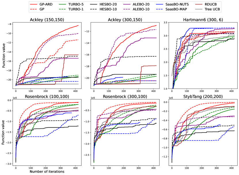
Synthetic Benchmarks. We considered four popular synthetic functions: Ackley, Rosenbrock, Hartmann6, and Stybtang. Definitions of these functions are provided in Section A.1 of the Appendix. Each task is represented by $\text{Fun}(d,d^{\prime})$, where $d$ is the input dimension that the BO methods optimize for, and $d^{\prime}$ is the number of effective variables ($d^{\prime}\leq d$). The target function is computed using the first $d^{\prime}$ variables. The benchmarks and the structures within the target functions are summarized in Table 1.

$\text{Fun}(d,d^{\prime})$	Structure
Ackley(300, 150)	Partial variable dependency
Rosenbrok(300, 100)	Partial variable dependency
	Nonoverlap additive decomposition
Hartmann6(300,6)	Partial variable dependency
Rosenbrock(100, 100)	Nonoverlap additive decomposition
Stybtang(200, 200)
Ackley(150, 150)	None

Table 1: Synthetic benchmarks and the structures within the target function: $d$ is the input dimension, and $d^{\prime}$ is the number of effective variables to compute the target function.

Real-World Benchmarks. We employed the following real-world benchmark problems.

• Mopta08 (124)  (Jones, 2008), a vehicle design problem. The objective is to minimize the mass of a vehicle with respect to 124 design variables, subject to 68 performance constraints. We followed (Eriksson and Jankowiak, 2021) to encode the constraints as a soft penalty, which is added into the objective.

• SVM (388) (Eriksson and Jankowiak, 2021), a hyper-parameter tuning problem that optimizes 3 regularization parameters and 385 length-scale parameters for a kernel support vector machine regression model.

• Rover (60), a rover trajectory planning problem from (Wang et al., 2018). The goal is to find an optimal trajectory determined by the location of 30 waypoints in a 2D environment.

• DNA (180) (vSehić et al., 2022), a hyper-parameter optimization problem that optimizes 180 regularization parameters for weighted lasso regression on an DNA dataset (Mills, 2020). Prior analysis (vSehić et al., 2022) shows that only around 43 variables are relevant to the target function.

• NAS201 (30)  (Dong and Yang, 2020), a neural architecture search problem on CIFAR-100 dataset.

• NN-Prune (151). We provided an additional real-world benchmark on neural network pruning (Blalock et al., 2020). We considered ResNet-152 (He et al., 2015), a deep residual network with 151 convolution layers and one linear layer, including more than 60 million parameters in total. We introduced a pruning rate $x_{i}$ for each convolution layer $i$. Given a global pruning ratio set to 0.5, the objective is to optimize the per-layer pruning rates to maximize the prediction accuracy on a test dataset after pruning and fine tuning. The details are given in Section A.2 of the Appendix.

Method	Structural Assumption
ALEBO, HESBO	Low-dim embedding
SaasBO	Partial variable dependency
RDUCB, Tree UCB	Additive function decomposition
GP-ARD, GP, TURBO	None

Table 2: BO methods and their structural assumption.

Methods. To execute the standard BO, we used GP regression with Matérn-5/2 ARD kernel (see (3)). We also tested with Matérn-5/2 kernel with a single length-scale parameter. We denoted these two choices as GP-ARD and GP, respectively. Throughout the experiments, we used UCB as the acquisition function where the exploration level $\lambda$ was set to 1.5. We used GPyTorch (Gardner et al., 2021) for surrogate training and BOTorch (Balandat et al., 2020) for acquisition function computation.

We compared with six state-of-the-art high-dimensional BO methods, including Tree UCB (Han et al., 2020), RDUCB (Ziomek and Bou-Ammar, 2023), HESBO (Nayebi et al., 2019), ALEBO (Letham et al., 2020), SaasBO (Eriksson and Jankowiak, 2021), and TURBO (Eriksson et al., 2020). The first five have been introduced in Section 3. TURBO is designed for a special scenario where the target function can be extensively evaluated (e.g., tens of thousands evaluations). This is not common in BO applications, as the function evaluation is typically deemed expensive, and one aims to evaluate the target function as few times as possible. TURBO searches for trust-regions in the input domain, learns a set of local GP models over each region, and then uses an implicit bandit strategy to decide which local optimization runs to continue. Table 2 summarizes the structural assumptions made by all the methods. We used the original implementation and default (recommended) settings for the competing methods. See details in Appendix Section A.3.

For each optimization task, we randomly queried the target function for 20 times to generate the initial data. We then ran each method for 400 steps for synthetic tasks and for 300 steps for real-world tasks. We tested TURBO with a single trust region and five trust regions, denoted by TURBO-1 and TURBO-5 respectively. For HESBO and ALEBO, we varied $d_{\text{emb}}\in\{10,20\}$ and denote the choice as HESBO/ALEBO-{10, 20}. For SaasBO, we performed tests using both NUTS and MAP estimation for surrogate training, denoted by SaasBO-NUTS and SaasBO-MAP, respectively. For standard BO, we trained the GP regression by maximizing the marginal likelihood using ADAM optimization (Kingma and Ba, 2014) (learning rate $0.1$ and 500 steps, as suggested in GPyTorch documents). We treated the mean function as a constant and jointly estimated it with the kernel parameters and noise variance.

4.2 Results and Discussion

4.2.1 Optimization Performance

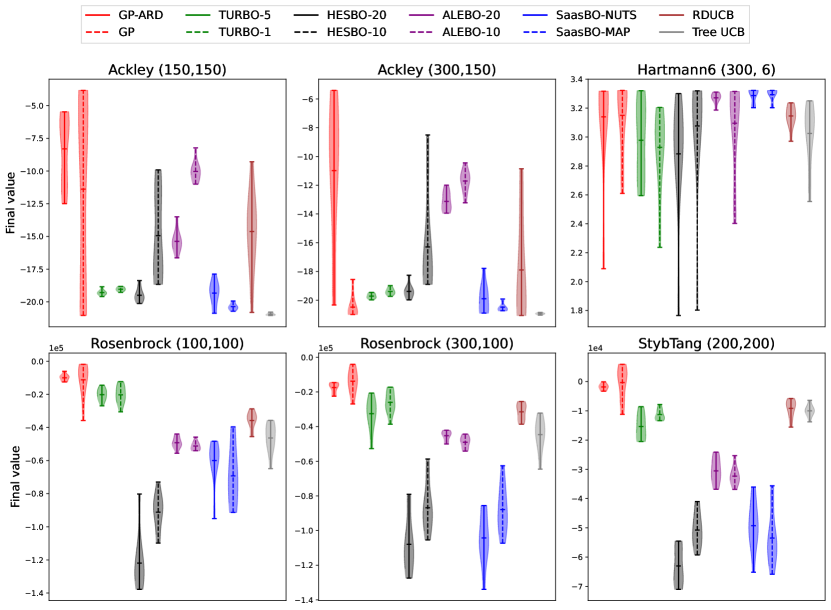
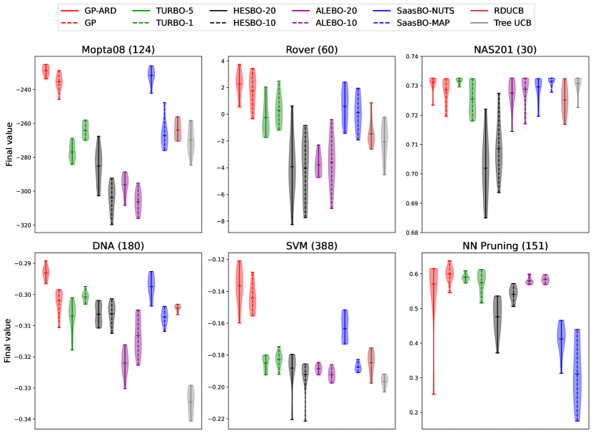
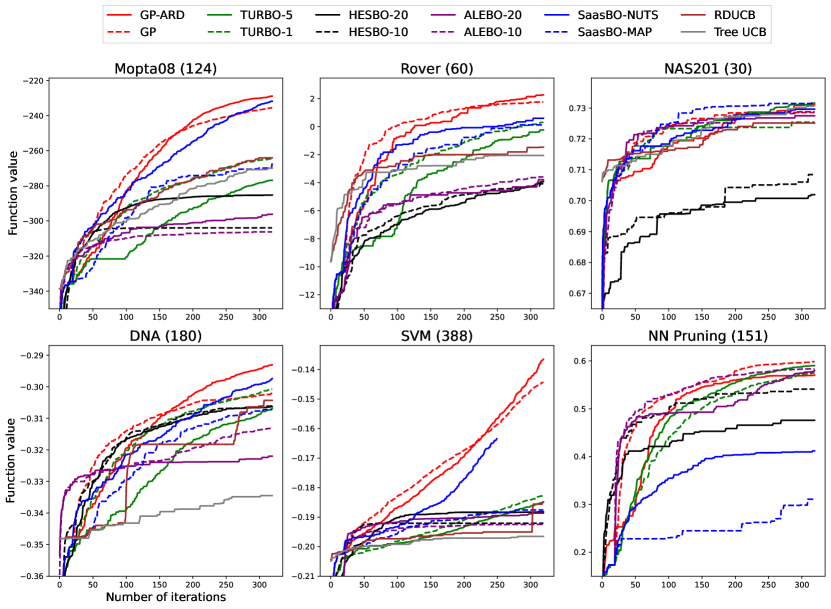
We present the ultimate optimization outcomes for synthetic benchmarks in Fig. 1 and for real-world benchmarks in Fig. 2. These are violin plots that illustrate the average of the obtained maximum function value over ten runs (the middle bar), the best (the top bar), the worst (the bottom bar), and the distribution of the obtained maximum (the shaded region). We can observe that on average, the standard BO with GP-ARD outperforms the competing high-dimensional BO methods in optimization every target function, often by a large margin, except that in the cases of Hartman6(300, 6) and NN-Prune, the performance with GP-ARD is slight worse (but still very close to) the best baseline(s).

It is noteworthy that the performance of the competing methods appears to be sensitive to the structure within the target function. For example, SaasBO imposes a strong inductive bias that only a small number of variables is related to the objective (via the usage of the horse-shoe prior). The target function in Hartman6(300, 6) and DNA aligns well with this assumption. As a result, SaasBO exhibits outstanding performance in both tasks. However, when the objective deviates from this assumption, as seen in cases like Ackley(150, 150), StybTang(200, 200), NN-Prune, and even Rosenbrock(300, 100), the performance of SaasBO experiences a dramatic drop. Another example is RDUCB and Tree-UCB, which assume that the target function can be decomposed as a summation of a group of functions, each over a small number of variables. RDUCB and Tree-UCB perform well in synthetic benchmarks that match this assumption, such as Rosenbrock(100, 100), Rosenbrock(300, 100), and StybTang(200, 200). However, their performance drops significantly in cases that do not align with their assumption, such as Ackley(150, 150) and Ackley(300, 150).

In contrast, GP-ARD exhibits much greater robustness to the structure of the target function. The standard BO with GP-ARD consistently ranks among the best in all tasks, regardless of whether the target function depends only on a subset of variables, can be decomposed, etc. Interestingly, the standard BO shows superior performance even when using a single length-scale parameter for GP, which closely matches GP-ARD across most tasks, except for Ackley(300, 150), GP struggled in finding right locations to query, leading to relative poor performance.

We also examined the runtime performance of each method. We report the maximum function value obtained throughout the optimization process in Fig. 5 and Fig. 6 of the Appendix. It is noticeable that after a few initial steps, the standard BO with GP-ARD (and also with GP in most cases) consistently generated superior queries, finding larger function values. Its curves are mostly above those of the competing methods, indicating a more efficient optimization of the target function. This trend is particularly evident in examples such as Rosenbrock(100, 100), StybTang(200, 200), Mopta08, Rover, SVM, and more.

The collective results demonstrate that the standard GP with ARD kernels is already effective for high-dimensional optimization. In comparison with using more complex surrogate models with additional assumptions, GP-ARD exhibits greater flexibility in adapting to the target function whose intrinsic structures are often agnostic in practice, and provides superior optimization results.

Figure 1: Optimization performance in synthetic benchmarks. The results were summarized from 10 runs.

Figure 2: Optimization performance in real-world problems. The results were summarized from 10 runs.

4.2.2 Surrogate Learning

Next, we explicitly evaluated the performance of the standard GP in learning high-dimensional functions to confirm if it can serve as a reliable surrogate model for high-dimensional BO. We sampled 300 training examples from all the six synthetic benchmark functions and four real-world benchmark tasks, including Mopta08 (124), Rover (60), DNA (180) and SVM (388). We sampled another 100 examples for testing. We compared with the surrogate models used in SaasBO and ALEBO (with $d_{\text{emb}}=10$ and $d_{\text{emb}}=20$). SaasBO was trained by NUTS. We repeated the experiment for five times, and evaluated the average test log-likelihood (LL), mean-square-error (MSE), and the standard deviation.

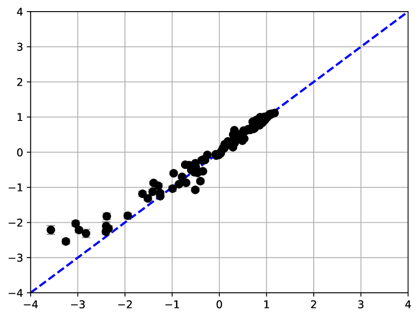
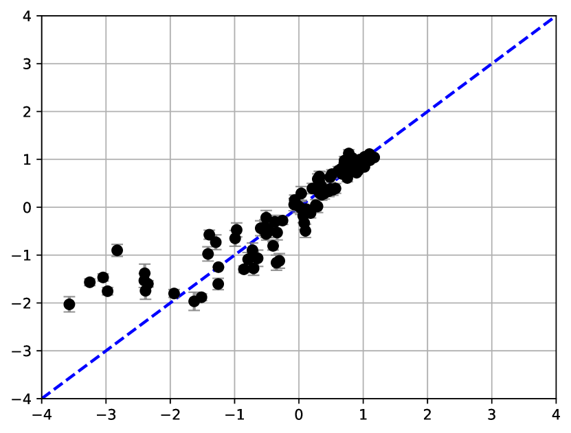
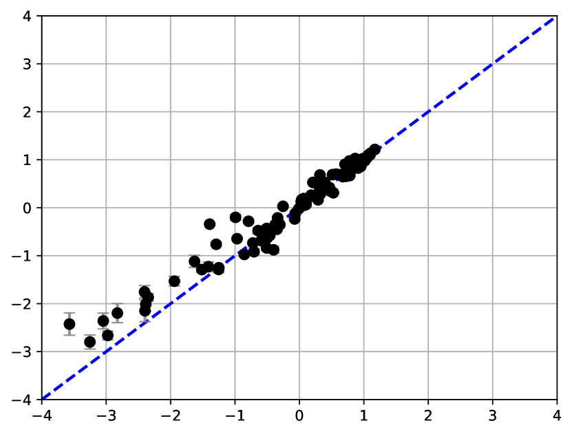
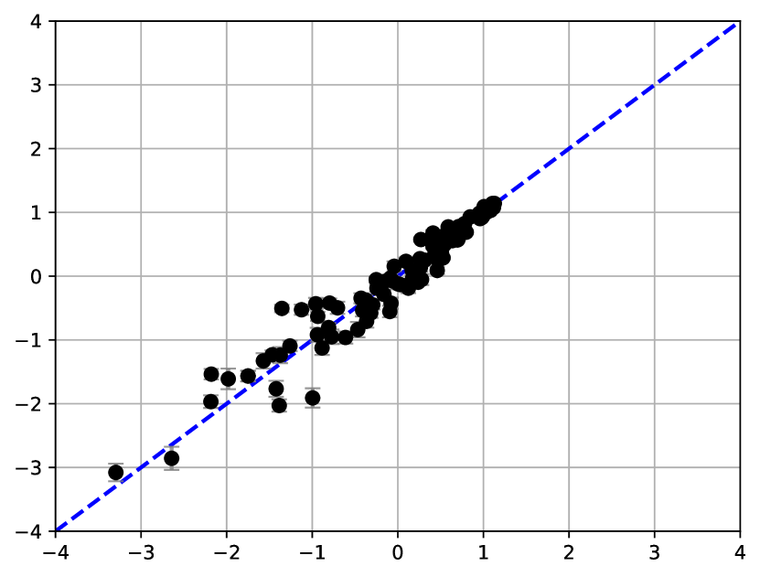
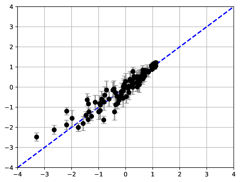
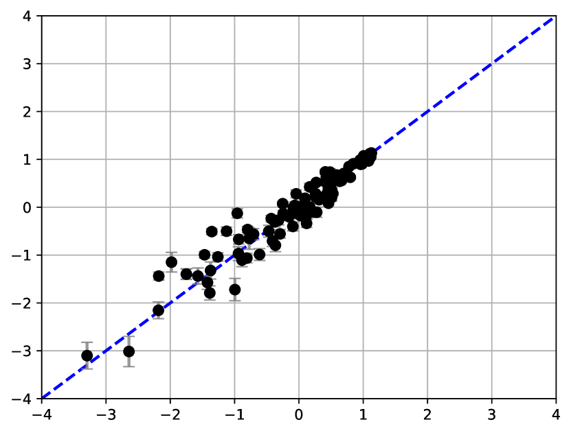
The results are reported in Table 3 and Appendix Table 5. We can see that in the vast majority of cases, GP-ARD achieves the largest test LL and the smallest MSE. GP-ARD and GP together nearly always outperforms SaasBO, ALEBO-10 and ALEBO-20. Notably, GP-ARD surpasses ALEBO by a substantial margin, while SaasBO exhibits a closer prediction accuracy. In addition, we examined the alignment between the prediction and the ground-truth across the test examples from Mopta and DNA. As illustrated in Fig. 4, the prediction (as well the predictive standard deviation) of GP-ARD matches the ground-truth equally as well as SaasBO-NUTS, with a slight improvement over GP (using a single length-scale parameter).

Together these results demonstrate that directly incorporating high-dimensional inputs into the kernel function does not necessarily compromise the learning performance. In other words, this implies that, even when the input space is high dimensional, commonly used kernels (e.g., the Matérn-5/2) remains expressive enough to capture the similarities in the space, allowing them to perform well in covariance modeling. On the contrary, enforcing (unnecessary) low-rank structures or sparsity might cause information loss, potentially detrimental to the learning performance. Our observation is consistent with the recent work in kernel operator learning (Batlle et al., 2024), where the standard kernel (GP) regression has demonstrated the state-of-the-art performance in learning function-to-function mappings. In this context, the input comprises of a discretized function, typically of very high-dimensionality (e.g., several thousands).

4.2.3 Computational Efficiency

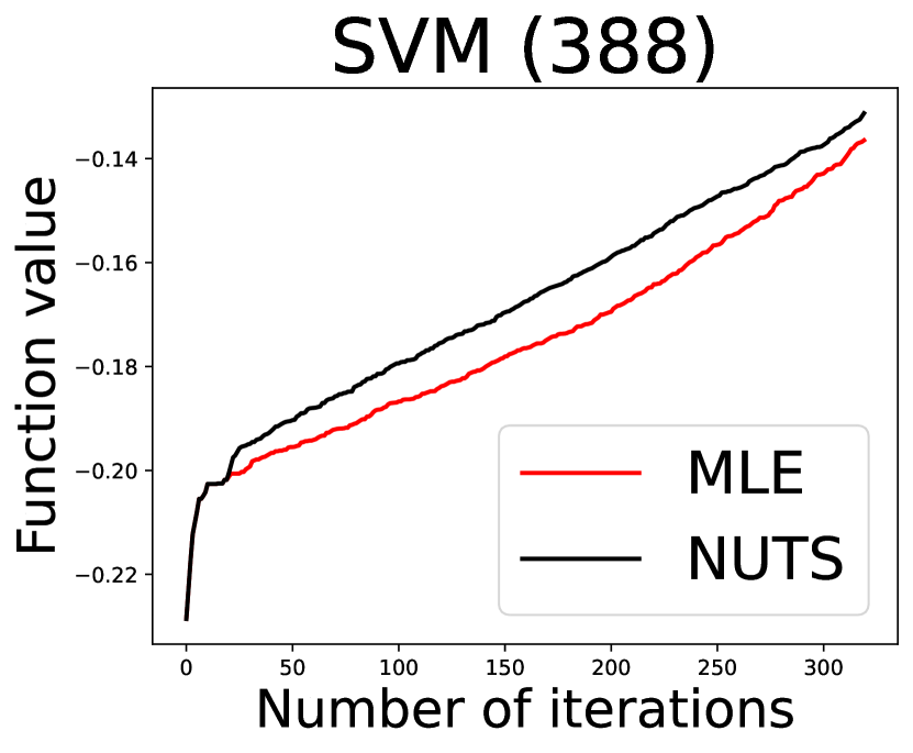
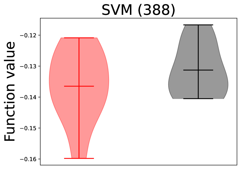
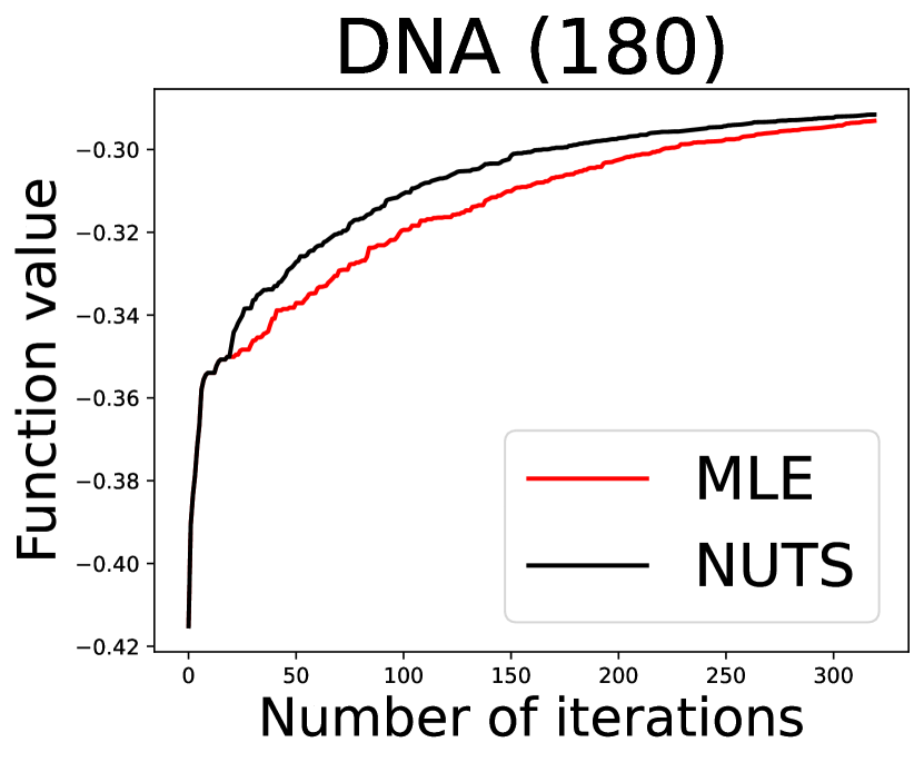
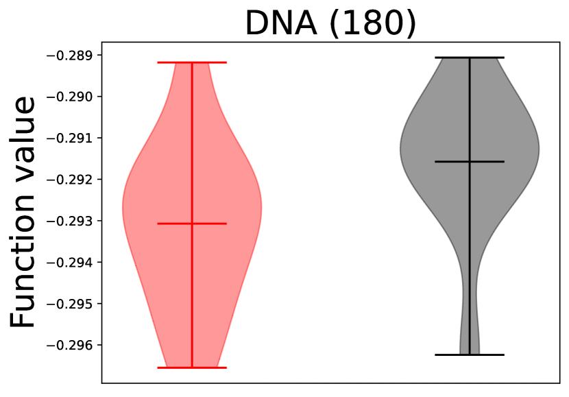
So far, in our BO loop, the GP model is trained via maximum likelihood estimation (MLE). Although the performance has been promising, it is worth investigating whether a full Bayesian approach would yield substantial improvements. In particular, we can use MCMC to perform posterior inference of the GP parameters, and then integrate them out during the prediction. We conducted another round of BO experiments. For each step, we used NUTS to train GP-ARD. We adopted the same settings as used in SaasBO-NUTS (Eriksson and Jankowiak, 2021), where the mean parameter is assigned the standard Gaussian prior $\mathcal{N}(0,1)$, amplitude $\text{Gamma}(2,0.15)$, and noise variance $\text{Gamma}(0.9,10)$. We then assigned a uniform prior over each length-scale, $\text{Uniform}(0.001,30)$. The number of warm up steps was set to 512, and after the warm up stage, we ran 256 steps, and selected the samples at every 16-th step as the posterior samples. We show the running and final optimization performance in Fig 3 , and Appendix Fig. 7. It can be observed that while NUTS contributes to a slight improvement in several tasks, the enhancement is very marginal. However, running NUTS is much more computationally costly compared to MLE. For example, on NAS201 and DNA, NUTS takes 68x and 40x running time than MLE in each optimization step. Therefore, for practical purposes, using maximum likelihood estimation (MLE) for Bayesian Optimization with GP-ARD appears sufficient. It is computationally efficient, and the sacrifice of optimization performance is minimal compared to much more costly training methods like NUTS.

By contrast, for more complex surrogate models, such as SaasBO, the MCMC based training might be more crucial for achieving good performance. As depicted in Fig. 2, SaasBO-NUTS demonstrates a substantial improvement over SaasBO-MAP across all real-world benchmarks, excluding NAS201. However, the computational cost of running SaasBO-NUTS is considerably higher, ranging from 5.4x (NAS201) to 33.9x (SVM, DNA) compared to the running time of SaasBO-MAP. This substantial increase in computational requirements may pose a severe bottleneck for practical usage. Detailed per-optimization-step running time for these methods are provided in Table 4 and Appendix Table 6.

Task	GP-ARD	GP	SaasBO	ALEBO-10	ALEBO-20
Mopta08(124)	0.613$\pm$0.156	-0.198$\pm$0.233	0.584$\pm$0.158	-1.176$\pm$0.080	-1.177$\pm$0.327
Rover(60)	-1.209$\pm$0.194	-0.908$\pm$0.068	-0.909$\pm$0.108	-1.270$\pm$0.094	-1.687$\pm$0.251
DNA(180)	0.005$\pm$0.175	-0.459$\pm$0.142	-0.066$\pm$0.225	-1.346$\pm$0.108	-1.572$\pm$0.432
SVM(388)	0.296$\pm$0.097	-0.090$\pm$0.065	0.160$\pm$0.113	-1.175$\pm$0.116	-1.077$\pm$0.148
Ackley(150, 150)	0.720$\pm$0.092	0.899$\pm$0.058	0.809$\pm$0.053	-0.852$\pm$0.091	-0.266$\pm$0.091
Ackley150(300, 150)	0.617$\pm$0.191	0.367$\pm$0.081	0.536$\pm$0.095	-0.870$\pm$0.097	-0.478$\pm$0.204
Hartmann6 (300, 6)	1.681$\pm$0.110	-1.031$\pm$0.117	2.152$\pm$0.971	-1.433$\pm$0.249	-1.689$\pm$0.411
Rosenbrock(100, 100)	0.602$\pm$0.069	0.172$\pm$0.099	0.553$\pm$0.084	-1.007$\pm$0.121	-0.854$\pm$0.355
Rosenbrock(300, 100)	0.436$\pm$0.098	-0.256$\pm$0.071	0.265$\pm$0.115	-1.118$\pm$0.065	-1.380$\pm$0.329
Stybtang(200, 200)	0.558$\pm$0.122	0.215$\pm$0.076	0.463$\pm$0.098	-1.050$\pm$0.099	-1.238$\pm$0.436

Table 3: Test log likelihood of each surrogate model. The results were averaged from five runs.

	Mopta08 (124)	Rover (60)	NAS201 (30)	DNA (180)	SVM (388)
GP-ARD	11.23	9.84	5.76	14.34	32.16
GP-ARD-NUTS	492.62	404.17	393.62	575.03	768.29
SaasBO-MAP	46.53	41.36	42.35	51.33	67.37
SaasBO-NUTS	985.76	375.06	229.07	1739.56	2269.50

Table 4: Average running time (in seconds) per optimization step in real-world benchmark tasks.

Figure 3: Optimization performance when using GP-ARD trained with maximum likelihood estimation (MLE) and NUTS on SVM (388) and DNA (180). The results were summarized from 10 runs.

(a) GP-ARD

(b) GP

(c) SaasBO-NUTS

Figure 4: Alignment between the prediction (y-axis) and ground-truth function values (x-axis). The top row is the results for Mopta08 (124) and the second row DNA (180).

5 Conclusion

A longstanding belief suggests that standard Gaussian process is insufficient to model high-dimensional functions, and Bayesian optimization with standard GP is expected to exhibit poor performance when optimizing functions with more than 20 variables. However, through a comprehensive investigation across various benchmark tasks, this paper challenges and overturns the prevailing notion.

Our findings reveal that standard GP excels in function estimation and uncertainty calibration, even when dealing with hundreds of input variables. Bayesian Optimization (BO) conducted with standard GP demonstrates remarkable performance in high-dimensional optimization, frequently outperforming existing high-dimensional BO methods by a substantial margin. Those methods, incorporating strong structural assumptions and employing more complex surrogate modeling, exhibit less robustness to various target functions, whose intrinsic structural properties are often agnostic in practice. Furthermore, the standard GP, benefiting from a parsimonious parameter space, can achieve satisfactory performance using only maximum likelihood estimation, thus eliminating the need for more computationally expensive Monte-Carlo methods in practical applications. Given these revelations, we advocate for a comprehensive exploration of the potential of the standard GP in high-dimensional optimization tasks.

Appendix

A More Experiment Details

A.1 Definition of Synthetic Functions

Stybtang. We used the following slightly-modified Stybtang function,

$$f({\bf x})=\frac{1}{2}\sum_{i=1}^{D}\left((x_{i}-c_{i})^{4}-16(x_{i}-c_{i})^{2}+5(x_{i}-c_{i})\right),$$

where ${\bf x}\in[-5,5]^{D}$, and we set $[c_{1},\dots,c_{D}]$ as an evenly spaced sequence in $[0,7.5]$ ($c_{1}=0$ and $c_{D}=7.5$). The optimum is at ${\bf x}^{\dagger}=[c_{1}-2.903534,\ldots,c_{D}-2.903534]$.

Rosenbrock. We used the following Rosenbrock function,

$$f({\bf x})=\sum_{i=1}^{D-1}\left[100\left((x_{i+1}-c_{i+1})-(x_{i}-c_{i})^{2}\right)^{2}+\left(1-(x_{i}-c_{i})\right)^{2}\right],$$

where ${\bf x}\in[-2.048,2.048]^{D}$. We set $[c_{1},...,c_{D}]$ as an evenly spaced sequence in $[-2,2]$, where $c_{1}=-2$ and $c_{D}=2$. The optimum is at $x^{\dagger}=[c_{1}+1,...,c_{D}+1]$.

Ackley. We used the Ackley function defined in (Surjanovic and Bingham, ),

$$f({\bf x})=-20\text{ exp}\left(-0.2\sqrt{\frac{1}{d}\sum_{i=1}^{d}x_{i}^{2}}\right)-\text{exp}\left(\frac{1}{d}\sum_{i=1}^{d}\text{cos}(2{\pi}x_{i})\right)+20+\text{exp}(1),$$

where each $x_{i}\in[-32.768,32.768]$ and the (global) optimum is at $x^{\dagger}=[0,\ldots,0]$.

Hartmann6. The function is given by

$$f({\bf x})=-\sum_{i=1}^{4}{\alpha}_{i}{\exp}\left(-\sum_{j=1}^{6}A_{ij}(x_{j}-P_{ij})^{2}\right),$$

where each $x_{i}\in[0,1]$, ${\bf A}=[A_{ij}]$ and ${\bf P}=[P_{ij}]$ are two pre-defined matrices as in (Surjanovic and Bingham, ). The global optimum is at ${\bf x}^{\dagger}=[0.20169,0.150011,0.476874,0.275332,0.6573]$.

Figure 5: Maximum Function Value Obtained vs. Number of Steps in synthetic benchmarks. The results were averaged from 10 runs.

Figure 6: Maximum Function Value Obtained vs. Number of Steps in real-world benchmarks. The results were averaged from 10 runs.

A.2 NN-Prune Details

Given specific per-layer pruning rates ${\bf x}=[x_{1},\ldots,x_{151}]$, the pruning procedure is as follows. The weights in each layer $i$ are first ranked according to their magnitudes, and the bottom $x_{i}$ portion of the weights are removed. The pruned network is then fine tuned on Tiny ImageNet (Le and Yang, 2015). The prediction accuracy after pruning and fine tuning on a separate test dataset is used as the target function. To respect the global pruning rate constraint $\alpha$, we add to the objective a soft penalty term $-\lambda\cdot\max(\alpha-\beta,0)$, where $\beta$ is the global pruning rate reflected from ${\bf x}$. Note that the penalty is only incurred when $\alpha>\beta$. When $\alpha<\beta$, namely, the network is pruned to be sparser than the expected level, the test accuracy typically experienced a significant decline. Consequently, the optimization process automatically adjusts to increase $\beta$. We set $\lambda=8.0$ to introduce a strong penalty. In our experiment, we employed $\alpha=0.5$.

A.3 Implementation

• ALEBO. We used ALEBO implementation shared by the Adaptive Experimentation (AX) Platform (version 0.2.2). The source code is at https://github.com/facebook/Ax/blob/main/ax/models/torch/alebo.py.

• HESBO. We used HESBO implementation of the original authors (https://github.com/aminnayebi/HesBO).

• TURBO. We used the original TURBO implementation (https://github.com/uber-research/TuRBO)

• SaasBO-NUTS. We used the original implementation of the authors (https://github.com/martinjankowiak/saasbo).

• SaasBO-MAP. The SaasBO implementation available to the public does not include the version using MAP estimation. We therefore implemented this method based on the original paper (Eriksson and Jankowiak, 2021). All the hyperparameter settings follow exactly the same as the original paper.

• RDUCB and Tree UCB. The implementation of both methods is publicly available at https://github.com/huawei-noah/HEBO/tree/master/RDUCB.

A.4 Computing Environment

We conducted the experimental investigations on a large computer cluster equipped with Intel Cascade Lake Platinum 8268 chips. For the NN-Prun problem, we ran the experiments on a Linux workstation, with a 16-core Intel 13900K CPU and one NVIDIA RTX 4090 GPU.

Task	GP-ARD	GP	SaasBO	ALEBO-10	ALEBO-20
Mopta08(124)	0.048$\pm$0.015	0.126$\pm$0.041	0.052$\pm$0.018	0.654$\pm$0.146	0.659$\pm$0.096
Rover(60)	0.493$\pm$0.126	0.449$\pm$0.108	0.453$\pm$0.121	0.813$\pm$0.168	1.266$\pm$0.352
DNA(180)	0.098$\pm$0.028	0.175$\pm$0.070	0.115$\pm$0.039	0.827$\pm$0.173	0.955$\pm$0.335
SVM(388)	0.042$\pm$0.010	0.098$\pm$0.012	0.061$\pm$0.017	0.624$\pm$0.159	0.493$\pm$0.132
Ackley(150, 150)	0.010$\pm$0.003	0.004$\pm$0.001	0.004$\pm$0.001	0.367$\pm$0.074	0.102$\pm$0.015
Ackley(300, 150)	0.010$\pm$0.003	0.018$\pm$0.004	0.010$\pm$0.002	0.360$\pm$0.109	0.177$\pm$0.075
Hartmann6(300, 6)	0.020$\pm$0.009	0.769$\pm$0.124	0.077$\pm$0.045	1.012$\pm$0.154	1.286$\pm$0.210
Rosenbrock(100, 100)	0.049$\pm$0.006	0.124$\pm$0.020	0.062$\pm$0.008	0.601$\pm$0.095	0.807$\pm$0.248
Rosenbrock(300, 100)	0.048$\pm$0.012	0.202$\pm$0.035	0.073$\pm$0.021	0.568$\pm$0.057	1.290$\pm$0.882
Stybtang(200, 200)	0.040$\pm$0.014	0.078$\pm$0.012	0.044$\pm$0.014	0.502$\pm$0.066	0.861$\pm$0.329

Table 5: Mean Squared Error (MSE) of each surrogate model. The results were averaged over five runs.

	Rosenbrock	Ackley	Stybtang	Rosenbrock	Ackley	Hartmann6
	(100,100)	(150, 150)	(200, 200)	(300, 100)	(300, 150)	(300, 6)
GP-ARD	8.85	12.94	13.67	12.63	9.99	8.81
GP-ARD-NUTS	857.21	850.23	1120.28	1276.42	1049.78	948.25
SaasBO-MAP	70.17	70.69	66.35	100.79	85.86	85.72
SaasBO-NUTS	1294.90	1621.60	1511.99	1938.53	925.80	2204.54

Table 6: Average running time (in seconds) per optimization step on synthetic benchmark tasks.

Figure 7: Optimization performance when using GP-ARD trained with maximum likelihood estimation (MLE) and NUTS on the rest of benchmarks. The results were summarized from 10 runs.

References

- Balandat et al. (2020) Maximilian Balandat, Brian Karrer, Daniel R. Jiang, Samuel Daulton, Benjamin Letham, Andrew Gordon Wilson, and Eytan Bakshy. Botorch: A framework for efficient monte-carlo bayesian optimization, 2020.
- Batlle et al. (2024) Pau Batlle, Matthieu Darcy, Bamdad Hosseini, and Houman Owhadi. Kernel methods are competitive for operator learning. Journal of Computational Physics, 496:112549, 2024.
- Blalock et al. (2020) Davis Blalock, Jose Javier Gonzalez Ortiz, Jonathan Frankle, and John Guttag. What is the state of neural network pruning?, 2020.
- Carvalho et al. (2009) Carlos M Carvalho, Nicholas G Polson, and James G Scott. Handling sparsity via the horseshoe. In Artificial intelligence and statistics, pages 73–80. PMLR, 2009.
- Dong and Yang (2020) Xuanyi Dong and Yi Yang. Nas-bench-201: Extending the scope of reproducible neural architecture search, 2020.
- Eriksson and Jankowiak (2021) David Eriksson and Martin Jankowiak. High-dimensional bayesian optimization with sparse axis-aligned subspaces, 2021.
- Eriksson et al. (2020) David Eriksson, Michael Pearce, Jacob R Gardner, Ryan Turner, and Matthias Poloczek. Scalable global optimization via local bayesian optimization, 2020.
- Frazier (2018) Peter I. Frazier. A tutorial on bayesian optimization, 2018.
- Gardner et al. (2021) Jacob R. Gardner, Geoff Pleiss, David Bindel, Kilian Q. Weinberger, and Andrew Gordon Wilson. Gpytorch: Blackbox matrix-matrix gaussian process inference with gpu acceleration, 2021.
- Han et al. (2020) Eric Han, Ishank Arora, and Jonathan Scarlett. High-dimensional bayesian optimization via tree-structured additive models, 2020.
- He et al. (2015) Kaiming He, Xiangyu Zhang, Shaoqing Ren, and Jian Sun. Deep residual learning for image recognition, 2015.
- Hoffman et al. (2014) Matthew D Hoffman, Andrew Gelman, et al. The No-U-Turn sampler: adaptively setting path lengths in Hamiltonian Monte Carlo. J. Mach. Learn. Res., 15(1):1593–1623, 2014.
- Jones (2008) Donald R Jones. Large-scale multi-disciplinary mass optimization in the auto industry. In MOPTA 2008 Conference (20 August 2008), volume 64, 2008.
- Jones et al. (1998) Donald R. Jones, Matthias Schonlau, and William J. Welch. Efficient global optimization of expensive black-box functions. Journal of Global Optimization, 13:455–492, 1998. URL https://api.semanticscholar.org/CorpusID:263864014.
- Kandasamy et al. (2016) Kirthevasan Kandasamy, Jeff Schneider, and Barnabas Poczos. High dimensional bayesian optimisation and bandits via additive models, 2016.
- Kingma and Ba (2014) Diederik P Kingma and Jimmy Ba. Adam: A method for stochastic optimization. arXiv preprint arXiv:1412.6980, 2014.
- Le and Yang (2015) Ya Le and Xuan S. Yang. Tiny imagenet visual recognition challenge. 2015. URL https://api.semanticscholar.org/CorpusID:16664790.
- Letham et al. (2020) Benjamin Letham, Roberto Calandra, Akshara Rai, and Eytan Bakshy. Re-examining linear embeddings for high-dimensional bayesian optimization, 2020.
- Li et al. (2016) Chun-Liang Li, Kirthevasan Kandasamy, Barnabas Poczos, and Jeff Schneider. High dimensional bayesian optimization via restricted projection pursuit models. In Arthur Gretton and Christian C. Robert, editors, Proceedings of the 19th International Conference on Artificial Intelligence and Statistics, volume 51 of Proceedings of Machine Learning Research, pages 884–892, Cadiz, Spain, 09–11 May 2016. PMLR. URL https://proceedings.mlr.press/v51/li16e.html.
- Mills (2020) Peter Mills. Accelerating kernel classifiers through borders mapping. Journal of Real-Time Image Processing, 17(2):313–327, 2020.
- Mockus (2012) Jonas Mockus. Bayesian approach to global optimization: theory and applications, volume 37. Springer Science & Business Media, 2012.
- Moriconi et al. (2020) Riccardo Moriconi, Marc P. Deisenroth, and K. S. Sesh Kumar. High-dimensional bayesian optimization using low-dimensional feature spaces, 2020.
- Nayebi et al. (2019) Amin Nayebi, Alexander Munteanu, and Matthias Poloczek. A framework for Bayesian optimization in embedded subspaces. In Kamalika Chaudhuri and Ruslan Salakhutdinov, editors, Proceedings of the 36th International Conference on Machine Learning, volume 97 of Proceedings of Machine Learning Research, pages 4752–4761. PMLR, 09–15 Jun 2019. URL https://proceedings.mlr.press/v97/nayebi19a.html.
- Rolland et al. (2018) Paul Rolland, Jonathan Scarlett, Ilija Bogunovic, and Volkan Cevher. High-dimensional bayesian optimization via additive models with overlapping groups, 2018.
- Russo et al. (2018) Daniel J Russo, Benjamin Van Roy, Abbas Kazerouni, Ian Osband, Zheng Wen, et al. A tutorial on Thompson sampling. Foundations and Trends® in Machine Learning, 11(1):1–96, 2018.
- Snoek et al. (2012) Jasper Snoek, Hugo Larochelle, and Ryan P Adams. Practical bayesian optimization of machine learning algorithms. In Advances in neural information processing systems, pages 2951–2959, 2012.
- (27) S. Surjanovic and D. Bingham. Virtual library of simulation experiments: Test functions and datasets. Retrieved January 23, 2024, from http://www.sfu.ca/~ssurjano.
- Wang et al. (2018) Zi Wang, Clement Gehring, Pushmeet Kohli, and Stefanie Jegelka. Batched large-scale bayesian optimization in high-dimensional spaces, 2018.
- Wang et al. (2016) Ziyu Wang, Frank Hutter, Masrour Zoghi, David Matheson, and Nando de Freitas. Bayesian optimization in a billion dimensions via random embeddings, 2016.
- Williams and Rasmussen (2006) Christopher KI Williams and Carl Edward Rasmussen. Gaussian processes for machine learning, volume 2. MIT press Cambridge, MA, 2006.
- Ziomek and Bou-Ammar (2023) Juliusz Ziomek and Haitham Bou-Ammar. Are random decompositions all we need in high dimensional bayesian optimisation?, 2023.
- vSehić et al. (2022) Kenan vSehić, Alexandre Gramfort, Joseph Salmon, and Luigi Nardi. Lassobench: A high-dimensional hyperparameter optimization benchmark suite for lasso, 2022.