Supersymmetry dictated topology in periodic gauge fields and realization in strained and twisted 2D materials

Abstract

Supersymmetry (SUSY) of Hamiltonian dictates double degeneracy between a pair of superpartners (SPs) transformed by supercharge, except at zero energy where modes remain unpaired in many cases. Here we explore a SUSY of complete isospectrum between SPs – with paired zero modes – realized by 2D electrons in zero-flux periodic gauge fields, which can describe twisted or periodically strained 2D materials. We find their low-energy sector containing zero (or threshold) modes must be topologically non-trivial, by proving that Chern numbers of the two SPs have a finite difference dictated by the number of zero modes and energy dispersion in their vicinity. In $30^{\circ}$ twisted bilayer (double bilayer) transition metal dichalcogenides subject to periodic strain, we find one SP is topologically trivial in its lowest miniband, while the twin SP of identical dispersion has a Chern number of $1$ ($2$), in stark contrast to time-reversal partners that have to be simultaneously trivial or nontrivial. For systems whose physical Hamiltonian corresponds to the square root of a SUSY Hamiltonian, such as twisted or strained bilayer graphene, we reveal that topological properties of the two SUSY SPs are transferred respectively to the conduction and valence bands, including the contrasted topology in the low-energy sector and identical topology in the high-energy sector. This offers a unified perspective for understanding topological properties in many flat-band systems described by such square-root models.

I Introduction

The discoveries of superconductivity and correlated insulating phases in twisted bilayer graphene (TBG) Cao et al. (2018a, b) have stimulated significant research interests in twisted and strained 2D materials that exhibit long-wavelength periodic spatial modulations. Many intriguing phenomena that have been observed in TBG Andrei and MacDonald (2020); Balents et al. (2020); Kennes et al. (2021); Andrei et al. (2021); Lau et al. (2022) are made possible by its flat bands, which not only allow Coulomb interaction effects to stand out due to the narrow bandwidth but also host nontrivial band topology Tarnopolsky et al. (2019); Liu et al. (2019). Topological minibands with valley-opposite Chern numbers as dictated by time-reversal symmetry are also found in twisted homobilayer transition metal dichalcogenides (tTMDs) Wu et al. (2019); Yu et al. (2020); Zhai and Yao (2020); Pan et al. (2020); Devakul et al. (2021), which underlie the observed fractional quantum anomalous Hall effects in tMoTe₂ when intrinsic ferromagnetism arises from Coulomb exchange Park et al. (2023); Cai et al. (2023); Anderson et al. (2023); Zeng et al. (2023); Xu et al. (2023). Interestingly, the electronic and topological properties of both TBG and tTMDs can be connected to periodic gauge fields. In TBG the relations between flat-bands and lowest Landau levels (LLs) are widely noted Tarnopolsky et al. (2019); Liu et al. (2019); Ledwith et al. (2020); Wang et al. (2021); Popov and Milekhin (2021), while in tTMDs the miniband topology can be attributed to an Abelian gauge field corresponding to the real-space Berry curvature acquired in the moiré Yu et al. (2020).

Supersymmetry (SUSY) is an active topic of research in theoretical physics. In quantum systems with SUSY Junker (2019), superpartners (SPs) with identical energy spectrum can emerge, reminiscent of the time-reversal partners represented by the two valleys in graphene or TMDs, whereas SPs are related by transformation known as supercharges. Initially proposed to relate fermions and bosons as SPs Volkov and Akulov (1973); Wess and Zumino (1974a, b); Haag et al. (1975), SUSY has been extended to encompass transformations between eigenstates of quantum Hamiltonians in general, providing a powerful tool across various frontiers of physics Junker (2019). Lately, there has been a surge of interest on the topological properties of lattice models that either exhibit SUSY or have indirect link to it com (a). Examples include topological mechanical lattices Kane and Lubensky (2014); Attig et al. (2019); Roychowdhury et al. (2022) and square-root topological materials Arkinstall et al. (2017); Ezawa (2020); Mizoguchi et al. (2020); Yoshida et al. (2021). A notable but not entirely unexpected finding is the two SPs can identically exhibit nontrivial topology in some high-energy sector Roychowdhury et al. (2022); Yoshida et al. (2021), which relies on the property that supercharges can transform SPs into each other at non-zero energy. This transformation, however, breaks down for the zero-energy modes, whose presence is required for defining an unbroken SUSY Junker (2019); com (b). Yet, the existing literature has mostly focused on models of either no zero mode or unpaired zero modes (e.g., a zero-energy flat band present only in one SP).

In this paper we present a systematic study on the topological properties of a SUSY of complete isospectrum between SPs, including paired zero modes, which can describe periodically strained TMDs on patterned substrate, as well as various flat-band superlattices, including e.g. TBG and strained bilayer graphene. We show that their low-energy sector containing zero (or threshold) mode must be topologically nontrivial, by proving a relation on the contrasted topology between SPs therein. Specifically, in the lowest-energy bands of the two SPs that feature identical dispersion, we show a finite difference in their Chern numbers dictated by the number of zero modes and energy dispersion in their vicinity, which guarantees that at least one SP is topologically nontrivial in the low-energy sector. We propose realization of such SUSY in $30^{\circ}$ twisted bilayer (double bilayer) TMDs with substrate-patterned periodic strain, where one SP is topologically trivial while the other has finite Chern number $1$ ($2$), albeit their complete degeneracy in the lowest-energy miniband. This is in stark contrast to the band topology in the circumstance of double degeneracy dictated by time-reversal symmetry. For systems whose physical Hamiltonian corresponds to the square root of a SUSY Hamiltonian, such as TBG and strained bilayer graphene, we reveal that topological properties of the two SUSY SPs are transferred respectively to the conduction and valence bands of the square-root physical Hamiltonian, including the contrasted topology in the low-energy sector and identical topology in the high-energy sector. As many flat-band systems are described by such square-root models, our findings offer a unified perspective for understanding their topological properties.

II Basics of SUSY

II.1 Pairing of superpartners between their positive energy states

In this work we consider SUSY Hamiltonian of the form

$$\begin{aligned} \mathcal{H}_{\text{susy}}=\begin{pmatrix}\mathbb{H}_{+}&0\\ 0&\mathbb{H}_{-}\end{pmatrix}=\begin{pmatrix}MM^{\dagger}&0\\ 0&M^{\dagger}M\end{pmatrix}\end{aligned},$$ (1)

where $M$ denotes a generic matrix. Its connection to the SUSY quantum mechanics Junker (2019) is revealed by rewriting

$$\mathcal{H}_{\text{susy}}=\{Q,\,Q^{\dagger}\},~{}$$ (2)

where

$$Q=\begin{pmatrix}0&M\\ 0&0\end{pmatrix}~{}~{}\text{and}~{}~{}Q^{\dagger}=\begin{pmatrix}0&0\\ M^{\dagger}&0\end{pmatrix}$$ (3)

are the complex supercharges (or SUSY generators). One can readily verify that

$$\{Q,\,Q\}=\{Q^{\dagger},\,Q^{\dagger}\}=[\mathcal{H}_{\text{susy}},\,Q]=[\mathcal{H}_{\text{susy}},\,Q^{\dagger}]=0.$$ (4)

These relations and Eq. (2) define the superalgebra and a SUSY quantum system Junker (2019). Such a SUSY system contains two parts ($\mathbb{H}_{\pm}$), and particles characterized by $\mathbb{H}_{+}\psi_{+}=\mathcal{E}_{+}\psi_{+}$ and $\mathbb{H}_{-}\psi_{-}=\mathcal{E}_{-}\psi_{-}$ are considered as superpartners (SPs) of each other. The eigenvectors of $\mathcal{H}_{\text{susy}}$ can be expressed in terms of $\psi_{\pm}$ as $\Psi_{+}=(\psi_{+},\,0)^{T}$ and $\Psi_{-}=(0,\,\psi_{-})^{T}$.

A SUSY system has several characteristic properties. First, as $\mathcal{H}_{\text{susy}}=\{Q,\,Q^{\dagger}\}$, its eigenenergies are non-negative. Second, the relation $[\mathcal{H}_{\text{susy}},\,Q]=[\mathcal{H}_{\text{susy}},\,Q^{\dagger}]=0$ dictates that any positive eigenvalue, i.e. $\mathcal{E}>0$, must have a pair of eigenstates from the two SPs respectively, satisfying $\mathcal{H}_{\text{susy}}\Psi_{\pm}=\mathcal{E}\Psi_{\pm}$. They can transform into each other via the supercharges $\Psi_{+}=Q\Psi_{-}/\sqrt{\mathcal{E}}$ and $\Psi_{-}=Q^{\dagger}\Psi_{+}/\sqrt{\mathcal{E}}$, or equivalently,

$$\psi_{+}=\frac{1}{\sqrt{\mathcal{E}}}M\psi_{-},~{}~{}\psi_{-}=\frac{1}{\sqrt{\mathcal{E}}}M^{\dagger}\psi_{+}.$$ (5)

The zero modes, $\Psi_{+}^{0}=(\psi_{+}^{0},\,0)^{T}$ and $\Psi_{-}^{0}=(0,\,\psi_{-}^{0})^{T}$, of the SUSY system are the ones annihilated by the supercharges, $M^{\dagger}\psi_{+}^{0}=0$ and $M\psi_{-}^{0}=0$. Thus the transformation connecting the SPs in Eq. (5) fails for the zero modes. This indicates that the zero-energy modes may remain unpaired or even be absent com (b). The difference in the number of zero modes between the SPs is the Witten index, which can be employed to characterize the SUSY systems.

II.2 Isospectrum in a zero-flux periodic gauge field

A nontrivial scenario where SUSY emerges corresponds to 2D electrons in a gauge field. We consider $M$ and $M^{\dagger}$ given in terms of $(\pi_{x},\,\pi_{y})=\boldsymbol{p}+e\boldsymbol{A}$, where $\boldsymbol{p}$ is the momentum operator and $\boldsymbol{A}$ is the gauge potential:

$$\begin{aligned} M=\alpha_{N}(\pi_{x}-i\pi_{y})^{N}=\alpha_{N}\pi_{-}^{N}\\ M^{\dagger}=\alpha_{N}(\pi_{x}+i\pi_{y})^{N}=\alpha_{N}\pi_{+}^{N}\end{aligned}.$$ (6)

Here $N$ denotes a positive integer, $\alpha_{N}$ is a constant such that $MM^{\dagger}$ and $M^{\dagger}M$ have units of energy, and we have also defined $\pi_{\pm}=\pi_{x}\pm i\pi_{y}$. The SUSY Hamiltonian is then

$$\begin{aligned} \mathcal{H}_{\text{susy}}=\begin{pmatrix}\mathbb{H}_{+}&0\\ 0&\mathbb{H}_{-}\end{pmatrix}=\begin{pmatrix}\alpha_{N}^{2}\pi_{-}^{N}\pi_{+}^{N}&0\\ 0&\alpha_{N}^{2}\pi_{+}^{N}\pi_{-}^{N}\end{pmatrix}\end{aligned}.~{}$$ (7)

The out-of-plane gauge field $\boldsymbol{B}=B\hat{\boldsymbol{z}}$ satisfies $[\pi_{x},\,\pi_{y}]=-ie\hbar B$. In the following we will assume that the field is Abelian, the discussions will be extended to cover non-Abelian gauge fields later.

In the case of $N=1$, the model describes spin–$\frac{1}{2}$ 2D electrons in an out-of-plane magnetic field,

$$M=\frac{1}{\sqrt{2m}}\pi_{-},~{}~{}M^{\dagger}=\frac{1}{\sqrt{2m}}\pi_{+}~{}~{}(\text{when}~{}N=1),$$ (8)

and

$$\begin{aligned} \mathbb{H}_{\pm}^{(N=1)}=\frac{1}{2m}\pi_{\mp}\pi_{\pm}=\frac{1}{2m}(\boldsymbol{p}+e\boldsymbol{A})^{2}\pm\boldsymbol{\mu}_{B}\cdot\boldsymbol{B}\end{aligned},$$ (9)

where $\boldsymbol{\mu}_{B}=\frac{e\hbar}{2m}\hat{\boldsymbol{z}}$ is the Bohr magneton. Spin-up and spin-down electrons are SPs of each other in this case.

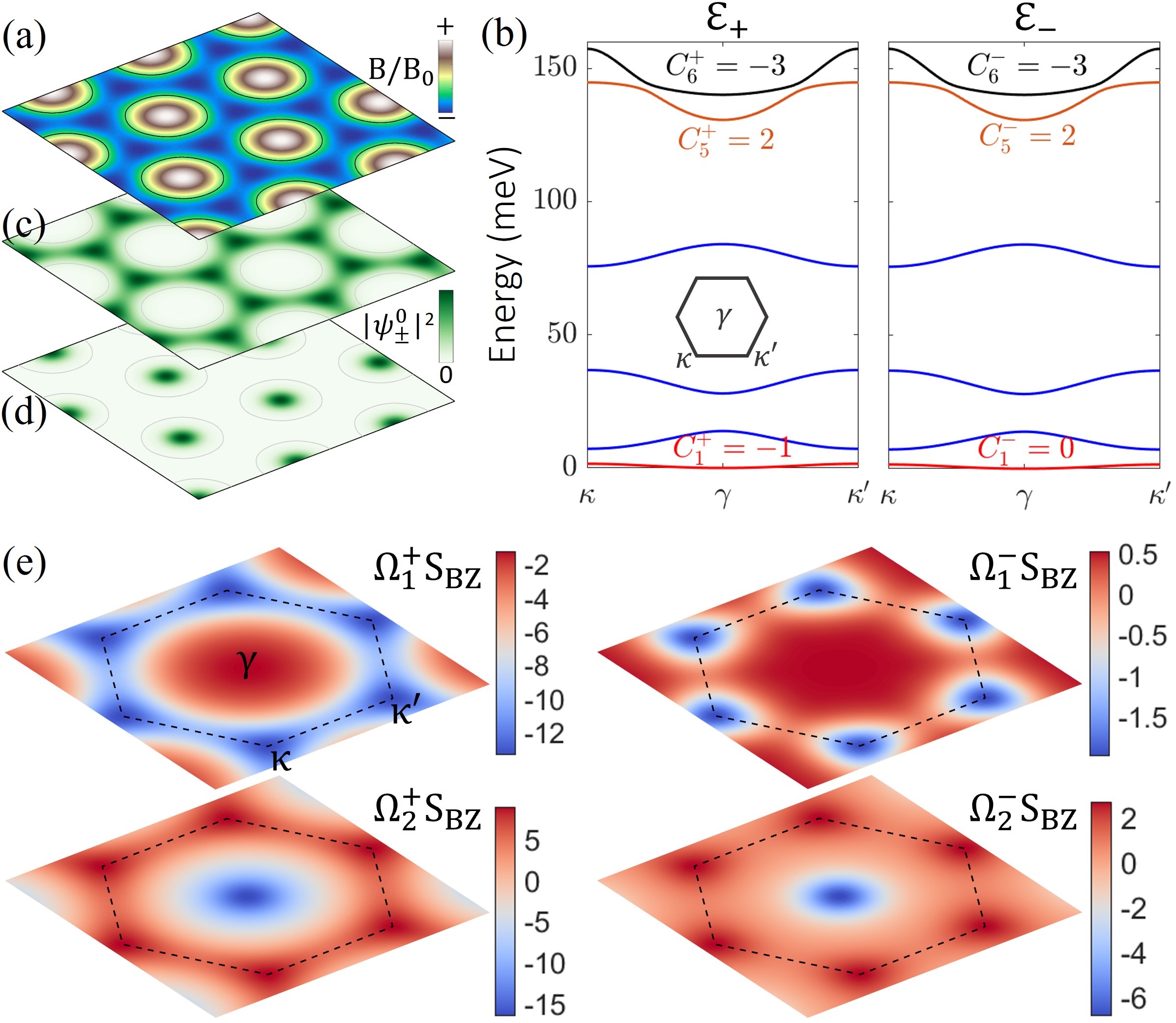
Figure 1: (a) A zero-flux periodic magnetic field, where black circles denote $B=0$ contours. (b) Energy bands and Chern numbers $C_{n}^{\pm}$ in the case of $N=1$ for $\mathcal{E}_{+}$ and $\mathcal{E}_{-}$, respectively. Blue bands have $C_{n}^{\pm}=0$. (c, d) Zero-mode distribution $|\psi_{\pm}^{0}|^{2}$ from $\mathcal{E}_{+}$ and $\mathcal{E}_{-}$, respectively. (e) Berry curvature of the first two bands of $\mathcal{E}_{\pm}$, the values are scaled by the area of the BZ $S_{BZ}$. Parameters: $B_{0}=120$ T, $L=14$ nm, $m=0.1$ free electron mass.

Information of the zero modes, i.e., their degeneracy and wave functions, can be obtained by solving $\pi_{\pm}\psi_{\pm}^{0}=0$, which depend on details of $\boldsymbol{B}$. Here we distinguish two scenarios:
(i) The situation of $\boldsymbol{B}$ with nonzero flux is known: the zero modes are spin-polarized with its degeneracy determined by the flux [see e.g., Fig. 3(a)], and notably, these features persist even when $\boldsymbol{B}$ is spatially nonuniform Aharonov and Casher (1979).
(ii) The scenario of periodic $\boldsymbol{B}$ with zero flux exhibits unique characteristics that have not been uncovered, and we will focus on them in this work. In this particular case, the two SPs each contains one unique zero mode, $\psi_{\pm}^{0}=c_{\pm}e^{\pm\phi}$, where $c_{\pm}$ are normalization constants, and the Coulomb gauge has been used with $\phi$ satisfying $e\boldsymbol{A}/\hbar=-\nabla\times(\phi\hat{\boldsymbol{z}})$ and $\partial_{\boldsymbol{r}}^{2}\phi=eB/\hbar$. Note that, although here we start with the case of $N=1$, the existence of such zero modes remains valid when $N>1$. Similar zero modes have also been found in graphene with a periodic gauge field Snyman (2009); Phong and Mele (2023) (also see Sec. V). Therefore, the spectra of two SPs are exactly the same when $\boldsymbol{B}$ is zero-flux periodic. This isospectral behavior is confirmed by solving Eq. (9) in a zero-flux $\boldsymbol{B}$ field of periodicity $L$ [Fig. 1(a)]: $\boldsymbol{B}(\boldsymbol{r})=\hat{z}B_{0}\sum_{i=1}^{3}\cos\left(\boldsymbol{b}_{i}\cdot\boldsymbol{r}\right)$, $\boldsymbol{b}_{1}=(\frac{\sqrt{3}}{2},\,-\frac{1}{2})\frac{4\pi}{\sqrt{3}L}$ and $\boldsymbol{b}_{i}=C_{3}^{i-1}\boldsymbol{b}_{1}$, where $C_{3}$ denotes the three-fold rotation operation. As expected, $\mathcal{E}_{+}$ and $\mathcal{E}_{-}$ each has one zero mode located at the $\gamma$ point [Fig. 1(b)].

III Contrasted topology in the isospectrum

Now we present the main findings of this work: the isospectral SPs in a zero-flux periodic $\boldsymbol{B}$ field are contrasted by distinct topology in their lowest bands that contain the zero modes, while all other bands have identical Chern numbers.

To figure out the relation of band Chern numbers of the SPs, it is convenient to look at their Berry connection $\boldsymbol{R}_{n}^{\pm}=i\braket{u_{n\boldsymbol{k}}^{\pm}}{\nabla_{\boldsymbol{k}}u_{n\boldsymbol{k}}^{\pm}}$, where $n=1,\,2,\cdots$ label the bands in ascending order of energy, and we denote the Bloch states of the SPs as $\ket{\psi_{\pm}}=e^{i\boldsymbol{k}\cdot\boldsymbol{r}}\ket{u_{n\boldsymbol{k}}^{\pm}}$. The Berry curvatures read $\Omega_{n}^{\pm}=[\nabla_{\boldsymbol{k}}\times\boldsymbol{R}_{n}^{\pm}]_{z}$, and the band Chern numbers are $C_{n}^{\pm}=\int_{\text{BZ}}\Omega_{n}^{\pm}\,d^{2}\boldsymbol{k}/(2\pi)$. By using the relation in Eq. (5), one finds that $\boldsymbol{R}_{n}^{+}$ and $\boldsymbol{R}_{n}^{-}$ differ by

$$\begin{aligned} \delta\boldsymbol{R}_{n}&=\boldsymbol{R}_{n}^{-}-\boldsymbol{R}_{n}^{+}\\ &=\frac{i}{\mathcal{E}_{n\boldsymbol{k}}}\braket{u_{n\boldsymbol{k}}^{+}}{M(\nabla_{\boldsymbol{k}}M^{\dagger})}{u_{n\boldsymbol{k}}^{+}}-i\frac{\hbar\boldsymbol{v}_{n\boldsymbol{k}}}{2\mathcal{E}_{n\boldsymbol{k}}}\end{aligned}.~{}$$ (10)

Here $\mathcal{E}_{n\boldsymbol{k}}>0$ is a common eigenenergy shared by $\ket{u_{n\boldsymbol{k}}^{\pm}}$, and $\boldsymbol{v}_{n\boldsymbol{k}}=(v_{n\boldsymbol{k}}^{x},\,v_{n\boldsymbol{k}}^{y})=\nabla_{\boldsymbol{k}}\mathcal{E}_{n\boldsymbol{k}}/\hbar$ is the band velocity. In the presence of zero modes, $\delta\boldsymbol{R}_{n}$ becomes singular as $\mathcal{E}_{n\boldsymbol{k}}\rightarrow 0$, thus different topology is expected between the $n=1$ bands of the SPs.

Consider $M$ and $M^{\dagger}$ given in Eq. (6), one straightforwardly finds

$$\delta\boldsymbol{R}_{n}=\frac{\hbar}{2\mathcal{E}_{n\boldsymbol{k}}}(v_{n\boldsymbol{k}}^{y},\,-v_{n\boldsymbol{k}}^{x}).$$ (11)

For any band except the first (i.e., $n>1$), since $\mathcal{E}_{n\boldsymbol{k}}\neq 0$, $\delta\boldsymbol{R}_{n}$ is well-behaved and periodic in the entire Brillouin zone (BZ), so from Stokes’ theorem, one readily identifies that the difference between the Chern numbers of the two SPs must vanish:

$$C_{n}^{+}-C_{n}^{-}=0,~{}~{}\text{for $n>1$}.$$ (12)

Note that although the SPs have identical dispersion and Chern numbers, their Berry curvatures in general differ,

$$\Omega_{n}^{-}-\Omega_{n}^{+}=-\frac{\hbar}{2}\nabla\cdot\frac{\boldsymbol{v}_{n\boldsymbol{k}}}{\mathcal{E}_{n\boldsymbol{k}}},~{}~{}\text{for $n>1$}$$ (13)

as shown by the example in Fig. 1(e). This is in contrast to the situation in some lattice models connected by SUSY, where identical Berry curvatures have been found Roychowdhury et al. (2022). In the present case, Berry curvatures of the SPs can be identical throughout the BZ when the bands become flat with $\boldsymbol{v}_{n\boldsymbol{k}}\equiv 0$.

Paired bands of identical dispersion having the same topology as dictated by Eq. (12) are intriguing but not that surprising, e.g., it is reminiscent of the pairing of Landau levels in constant magnetic field [Fig. 3(a)]. The results thus far, however, do not address the presence of the zero modes, which are crucial ingredients of SUSY com (b).

Remarkably, since Eq. (10) is singular at the zero energy, topology of the $n=1$ bands of the SPs are distinct. Like in the case of Fig. 1(b), let us assume for now that there is one zero mode on each of $\mathcal{E}_{\pm}$ and it locates at the $\gamma$ point. As $\delta\boldsymbol{R}_{1}$ is singular when $\boldsymbol{k}\rightarrow\gamma$, while it is well-defined and periodic elsewhere, its line integral on a circle enclosing the zero mode will yield the difference of the Chern number [Fig. 2(a)]:

$$\begin{aligned} C_{1}^{-}-C_{1}^{+}=\frac{1}{2\pi}\oint_{\text{O}_{\gamma}}\delta\boldsymbol{R}_{1}\cdot d\boldsymbol{l}=\frac{1}{4\pi}\int^{2\pi}_{0}\frac{k}{\mathcal{E}_{1\boldsymbol{k}}}\frac{\partial\mathcal{E}_{1\boldsymbol{k}}}{\partial k}\,d\varphi\end{aligned},$$ (14)

where $\text{O}_{\gamma}$ denotes a circle centered at $\gamma$. In the second equality, $\boldsymbol{k}$ is understood to be on the circle and measured from $\gamma$, and $\varphi$ is its polar angle. Being the difference of two Chern numbers, the result must be an integer. In particular, when the low-energy dispersion $\mathcal{E}_{1\boldsymbol{k}}\propto k^{2\mathbb{N}}$ around the zero mode, $\mathbb{N}$ a positive integer, we have,

$$C_{1}^{+}-C_{1}^{-}=\mathbb{N}.$$ (15)

This key finding of the work is schematically summarized in Fig. 2(a). For typical 2D electron systems with quadratic dispersion at low energies, $C_{1}^{-}-C_{1}^{+}=1$. Although the individual value of $C_{1}^{\pm}$ cannot be determined here, a nonzero difference ($C_{1}^{-}-C_{1}^{+}\neq 0$) guarantees that at least one of the bands is topologically nontrivial.

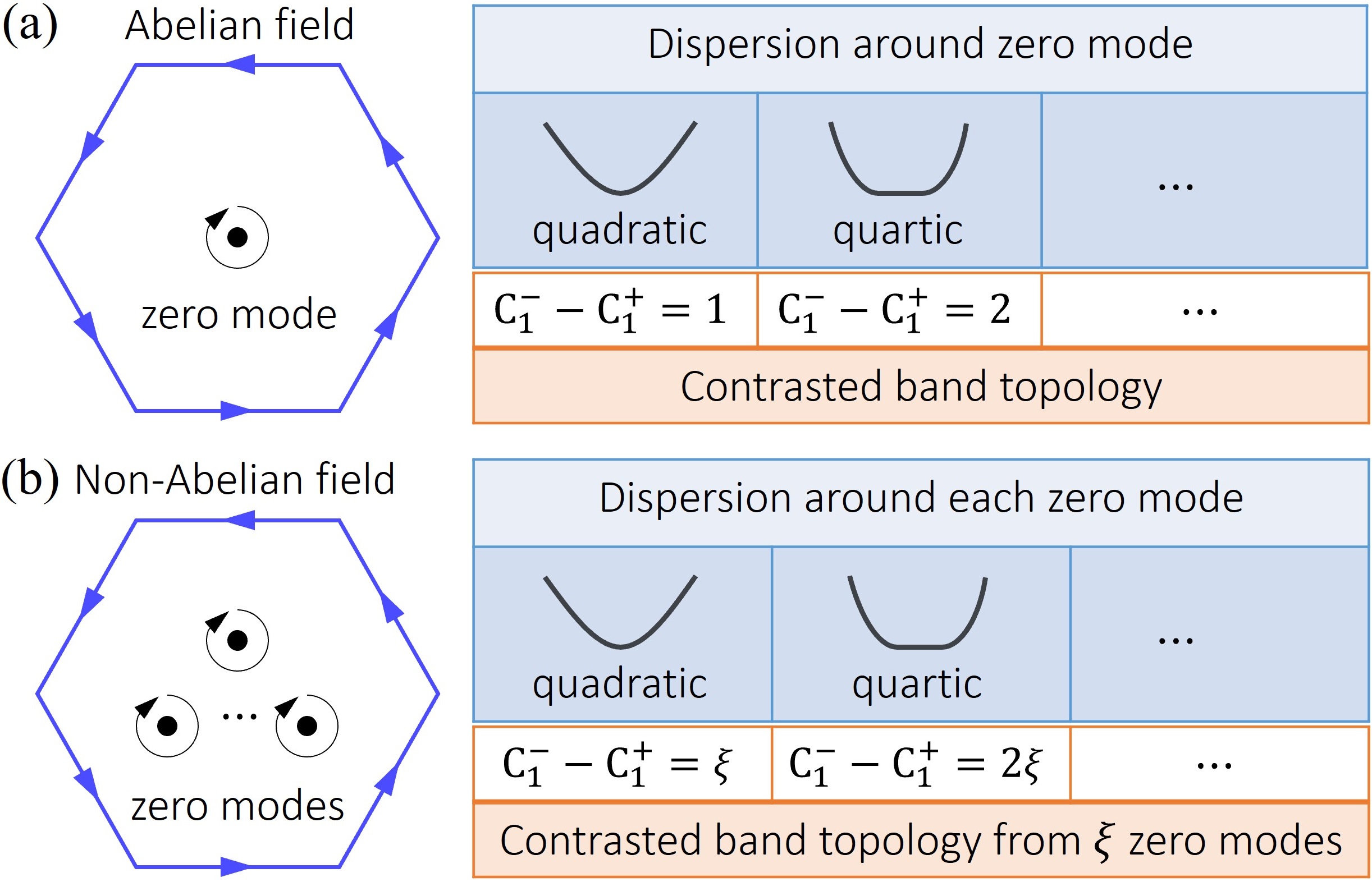
Figure 2: (a) Schematics of Brillouin zone (blue hexagon) with one zero mode (black dot) at the center for the case of an Abelian gauge field. The Chern number difference $C_{1}^{-}-C_{1}^{+}$ due to different low-energy dispersion around the zero mode is summarized. (b) Similar to case (a) but with multiple zero modes, which might occur when the field is non-Abelian. The Chern number difference $C_{1}^{-}-C_{1}^{+}$ increases with the number of zero modes.

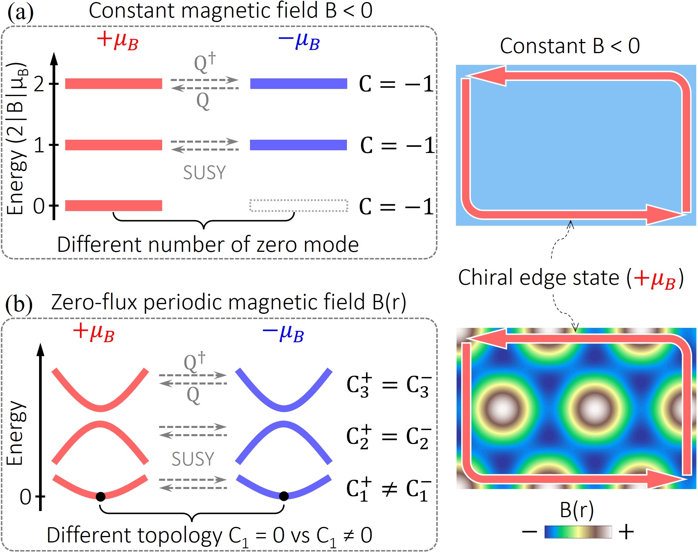
Figure 3: (a) Landau levels in a uniform field. The mismatched zero-energy level indicates unequal number of zero modes for the two spin species. (b) Fully spin-symmetric spectra in a zero-flux periodic field. The first bands of the two spin species each has one zero mode (black dot), but feature distinct band topology. Note that both (a) and (b) support fully spin-polarized chiral edge state inside the first energy gap.

Figure 1(b) shows the band Chern numbers for the example of Eq. (9) when the $\boldsymbol{B}$ field is zero-flux periodic. As expected, $C_{n}^{+}=C_{n}^{-}$ when $n>1$. This part is reminiscent of Landau levels (LLs) at nonzero energies in a uniform field [see schematics in Fig. 3(a)], but clear distinctions can be identified: here the Chern numbers can vary from band to band, and their values are not restricted to $\pm 1$. Most importantly, we find that in the lowest band $n=1$, one spin is topologically trivial ($C_{1}^{-}=0$) while its isospectral SP is nontrivial ($C_{1}^{+}=-1$), as dictated by Eq. (15) for the quadratic dispersion. This contrasted topology [Fig. 1(b)] suggests that zero-flux periodic $\boldsymbol{B}$ fields support spin-polarized chiral edge states in the gaps, akin to the situation in a uniform field. But importantly, this is made possible by the distinct topology in bands that have identical dispersion ($\mathcal{E}_{1\boldsymbol{k}}^{+}=\mathcal{E}_{1\boldsymbol{k}}^{-}$ but $C_{1}^{+}\neq C_{1}^{-}$), instead of the lack of zero-energy LL for one spin species in a uniform field. These significant distinctions between uniform and zero-flux periodic fields are schematically summarized in Figs. 3(a) vs (b). For a general periodic $\boldsymbol{B}$ field without net flux, one can speculate that the lowest bands of the SPs are always contrasted by Chern numbers $0$ vs $\pm 1$, thus the presence of chiral edge states with a definite spin in the first gap [Fig. 3(a)] is preserved when $\boldsymbol{B}$ evolves from a uniform one to zero-flux periodic ones [Fig. 3(b)].

In Sec. S1 of Supplementary Material sup we show more examples of band structures and topology by comparing to similar systems without SUSY. The results imply that the electronic and topological properties of systems with SUSY are more robust against variations in the $\boldsymbol{B}$ field (e.g., intensity and period). Also, given one $\boldsymbol{B}$ field, larger Chern number difference in the lowest band ($C_{1}^{-}-C_{1}^{+}$) can be realized by considering the cases of $N>1$ in Eq. (7), i.e. with non-quadratic dispersions. An example of such scenarios will be discussed in Sec. IV.2.

The contrasted topology $C_{1}^{+}\neq C_{1}^{-}$ is also accompanied by distinct wave function distributions. The zero mode $\psi_{+}^{0}$ ($\psi_{-}^{0}$) distribution is strongly correlated with that of the $\boldsymbol{B}$ field by primarily occupying regions where $B<0$ ($B>0$) Aharonov and Casher (1979); Snyman (2009). In fact, other states on the first band $\mathcal{E}_{1}^{+}$ ($\mathcal{E}_{1}^{-}$) also show similar distribution patterns. This can be easily understood from the Zeeman term in Eq. (9) Georgi et al. (2017): An electron with $+\boldsymbol{\mu}_{B}$ ($-\boldsymbol{\mu}_{B}$) has lower energy when it resides in the region with $B<0$ ($B>0$). Therefore, in the case of Fig. 1(a), $|\psi_{+}^{0}|^{2}$ occupy the region of $B<0$, showing a honeycomb network [Fig. 1(c)], and the band Chern number $C_{1}^{+}=-1$ is consistent with the sign of the underlying field; while $|\psi_{-}^{0}|^{2}$ shows features of localized dots [Fig. 1(d)] with $C_{1}^{-}=0$. Importantly, profile of the zero-modes, i.e., connected or localized, which is readily known via the Zeeman term, serves as a indicator for quickly identifying the topology of the $n=1$ bands. For example, when the sign of the $\boldsymbol{B}$ field in Fig. 1(a) is reversed, one can easily find $C_{1}^{+}=0$ vs $C_{1}^{-}=1$, thus the edge state in the first gap has opposite spin as expected and $C_{1}^{-}-C_{1}^{+}=1$ persists. It is interesting to notice that the Chern numbers change from $(C_{1}^{+},\,C_{1}^{-})=(-1,\,0)$ to $(C_{1}^{+},\,C_{1}^{-})=(0,\,1)$ on the lowest band after inverting the $\boldsymbol{B}$ field, which is in contrast to the simple sign reversal of Chern numbers on the other bands, i.e., $C_{n}^{\pm}(\boldsymbol{B})=-C_{n}^{\pm}(-\boldsymbol{B})$ when $n>1$.

We now comment on the scenario of non-Abelian gauge field $\boldsymbol{B}$. In non-Abelian cases, Eq. (5) and the resultant Eq. (11) remain valid at nonzero energies. However, it should be noted that each SP may have multiple zero modes when $\boldsymbol{B}$ is non-Abelian (see example in Sec. V.2). Nevertheless, the line integral around each zero mode –like that in Eq. (14) and Fig. 2(a)– can be preformed. By adding up such individual contributions from all the zero modes, we obtain

$$C_{1}^{-}-C_{1}^{+}=\frac{1}{2\pi}\sum_{i}\oint_{\text{O}_{i}}\delta\boldsymbol{R}_{1}\cdot d\boldsymbol{l},$$ (16)

where $\text{O}_{i}$ denotes a circle enclosing the $i$-th zero mode, and each summand is determind by Eq. (15). Here we have assumed that the number of zero modes is limited and they are discretely distributed in the BZ. These results are schematically summarized in Fig. 2(b). Therefore, the main findings discussed in the above remain valid, and they can be applied to many other systems, which we will discuss in Sec. V.2.

IV Realization in perodically strained 2D semiconductors

Naively, one might expect that the discussed SUSY model [e.g., Eq. (9)] and the intriguing feature of isospectra with contrasted band topology can be easily realized by applying a periodic magnetic field to 2D electron systems. However, there exist two obstacles in experimental implementations: (i) It is technically challenging to generate smooth and periodic magnetic field landscapes Dong et al. (2022). (ii) A real magnetic field can couple to magnetic moments of various origins (e.g., spin, orbital, and valley Aivazian et al. (2015)), which introduces extra Zeeman terms that break SUSY. In the following, we will show that such difficulties can be circumvented by using periodically strained 2D semiconductors, e.g., TMDs. By employing strain-induced pseudo-magnetic field Vozmediano et al. (2010); Amorim et al. (2016); Naumis et al. (2017), and taking the advantage that it only couples to the valley magnetic moment Xiao et al. (2007), we show that it is possible to realize the SUSY systems discussed earlier.

IV.1 $30^{\circ}$ twisted bilayer TMDs for $N=1$ SUSY with quardatic dispersion

We will consider TMDs as an example below, but the discussions are also applicable for many other 2D semiconductors, e.g., graphene with a staggered potential or hBN. In monolayer TMDs, the low-energy carriers are governed by massive Dirac equations $h^{\text{1L}}_{\tau}=v\boldsymbol{\sigma}_{\tau}\cdot\boldsymbol{p}+\Delta\sigma_{z}$ in two inequivalent valleys labeled as $\tau K$, where $\tau=\pm$ is the valley index, $v$ is the Fermi velocity, and $\boldsymbol{\sigma}_{\tau}=(\tau\sigma_{x},\,\sigma_{y})$ Xiao et al. (2012). By introducing nonuniform strain patterns, giant pseudo-magnetic fields opposite in the two valleys can be generated Vozmediano et al. (2010); Amorim et al. (2016); Naumis et al. (2017). The Dirac Hamiltonian in the presence of strain pseudo-magnetic field becomes

$$H^{\text{D}}_{\tau}=v\boldsymbol{\sigma}_{\tau}\cdot(\boldsymbol{p}+\tau e\boldsymbol{A})+\Delta\sigma_{z},~{}$$ (17)

where $\tau\boldsymbol{A}$ is the strain vector potential and its details will be discussed later. Note that there might also exist strain-induced scalar potentials. We discuss such terms in Sec. S2 of Supplementary Material sup , and show that WSe₂ is an ideal candidate, in which such terms can be neglected. Importantly, profile of the pseudo-magnetic field, $\tau\boldsymbol{B}=\nabla\times(\tau\boldsymbol{A})$, can be controlled by tuning the strain distribution. Strain engineering in 2D materials Guinea et al. (2010); Tomori et al. (2011); Reserbat-Plantey et al. (2014); Jiang et al. (2017); Zhang et al. (2018a); Phong and Mele (2022); Mahmud et al. (2023) thus offers a solution to overcome the obstacle of generating patterned magnetic fields with zero flux.

The Dirac model $H^{\text{D}}_{\tau}$ describes charge carriers in both the conduction and valence bands. From experimental perspectives, for TMDs it is most natural to consider holes (h) near the valence band edge, which are described by

$$H^{h}_{\tau}\psi=[\frac{1}{2m}(\boldsymbol{p}+\tau e\boldsymbol{A})^{2}+\boldsymbol{\mu}_{\tau}^{h}\cdot(\tau\boldsymbol{B})]\psi=\varepsilon\psi$$ (18)

near the valence band edge in the limit of $\varepsilon\ll\Delta$. In this quadratic model, $\varepsilon$ is measured from the valence band edge, $m=\Delta/v^{2}$ is the effective mass, and $\boldsymbol{\mu}_{\tau}^{h}=-\tau\boldsymbol{\mu}_{B}$ is the valley magnetic moment Xiao et al. (2007) for holes. Note that a magnetic moment in the form of Bohr magneton naturally appears here, which is a characteristic of the low-energy behavior of the massive Dirac model. More importantly, the strain pseudo-magnetic field can only couple to this valley magnetic moment, but not other sources (e.g., spin and orbital Aivazian et al. (2015)). Therefore, the second challenge mentioned above for realizing SUSY is resolved.

IV.1.1 Layer-valley pseudospin realization of superpartners

We now propose a practical scheme to achieve SPs with contrasted band topology satisfying $C_{1}^{-}-C_{1}^{+}=1$. We first focus on the general ideas that are independent of details of the $\boldsymbol{B}$ fields. The proposal employs a bilayer geometry with layer-opposite strain pseudo-magnetic fields, i.e., $\boldsymbol{B}^{(1)}=-\boldsymbol{B}^{(2)}$, where the superscript is layer index. Then holes from opposite valleys of opposite layers form SPs [Fig. 5(b)]. To see this formally, we write the Hamiltonian in such configurations explicitly:

$$\begin{aligned} H^{h}_{\tau}(\text{layer 1})&=\frac{1}{2m}\left(\boldsymbol{p}+\tau e\boldsymbol{A}^{(1)}\right)^{2}+\boldsymbol{\mu}_{\tau}^{h}\cdot\left(\tau\boldsymbol{B}^{(1)}\right)\\ H^{h}_{-\tau}(\text{layer 2})&=\frac{1}{2m}\left(\boldsymbol{p}+\tau e\boldsymbol{A}^{(1)}\right)^{2}+\boldsymbol{\mu}_{-\tau}^{h}\cdot\left(\tau\boldsymbol{B}^{(1)}\right)\end{aligned},$$ (19)

where $-\boldsymbol{A}^{(2)}$ and $-\boldsymbol{B}^{(2)}$ have been replaced by $\boldsymbol{A}^{(1)}$ and $\boldsymbol{B}^{(1)}$ in layer 2, and interlayer coupling has been assumed to be negligible. Clearly, the only difference between the two lines lies in the magnetic moments, which are opposite to each other. Such a bilayer geometry thus realizes the SUSY model in Eq. (9).

IV.1.2 Twist control of strain induced pseudo-magnetic field on patterned substrate

Strained induced pseudo-magnetic field with the periodic landscape of Fig. 1(a) has been proposed in buckled graphene on NbSe₂ Mao et al. (2020). Pseudo-magnetic fields with similar profiles can also appear due to lattice relaxation in the moiré of H-type bilayer TMDs Enaldiev et al. (2020); Xie et al. (2022); com (c). However, strain originates from spontaneous atomic displacements in these scenarios, thus it is challenging to tune the pseudo-magnetic field (e.g., magnitude, period, profile), if not impossible. Alternatively, strain engineering can be implemented in a more controllable manner by using patterned substrates. This approach offers great flexibility in realizing different pseudo magnetic fields, mostly by properly designing the substrates with various landscapes Tomori et al. (2011); Reserbat-Plantey et al. (2014); Jiang et al. (2017); Zhang et al. (2018a); Phong and Mele (2022); Mahmud et al. (2023).

Here we highlight another important feature of substrate-assisted strain engineering: Given a pre-fabricated substrate with a fixed surface landscape, the periodic pseudo-magnetic field imprinted onto the deposited material can be controlled simply by rotating the material with respect to the substrate (Fig. 4). We will consider a TMD membrane following the surface of a patterned substrate modeled by $z(\boldsymbol{r})=z_{0}\sum_{i=1}^{3}\cos(\boldsymbol{b}_{i}\cdot\boldsymbol{r}+\frac{\pi}{12})$ as an example, where $\boldsymbol{b}_{1}=(\frac{\sqrt{3}}{2},\,-\frac{1}{2})\frac{4\pi}{\sqrt{3}L}$ and $\boldsymbol{b}_{i}=C_{3}^{i-1}\boldsymbol{b}_{1}$. This height profile is shown schematically in Fig. 4(a). We note that in-plane atomic displacements on the lattice could also occur after the deposition. But their details strongly depend on the specific experimental settings, e.g., whether the membrane is freely relaxed, or clamped on the edges, or fixed on extrema of the patterned substrate, etc Wehling et al. (2008); Guinea et al. (2010); Phong and Mele (2022). Here we neglect in-plane displacements for simplicity, which does not affect conclusions of the following discussions. The resultant strain tensor components on the lattice can then be obtained from its out-of-plane deformation, $\epsilon_{ij}=(\partial_{i}z)(\partial_{j}z)/2$, where $i,\,j\in\{x,\,y\}$.

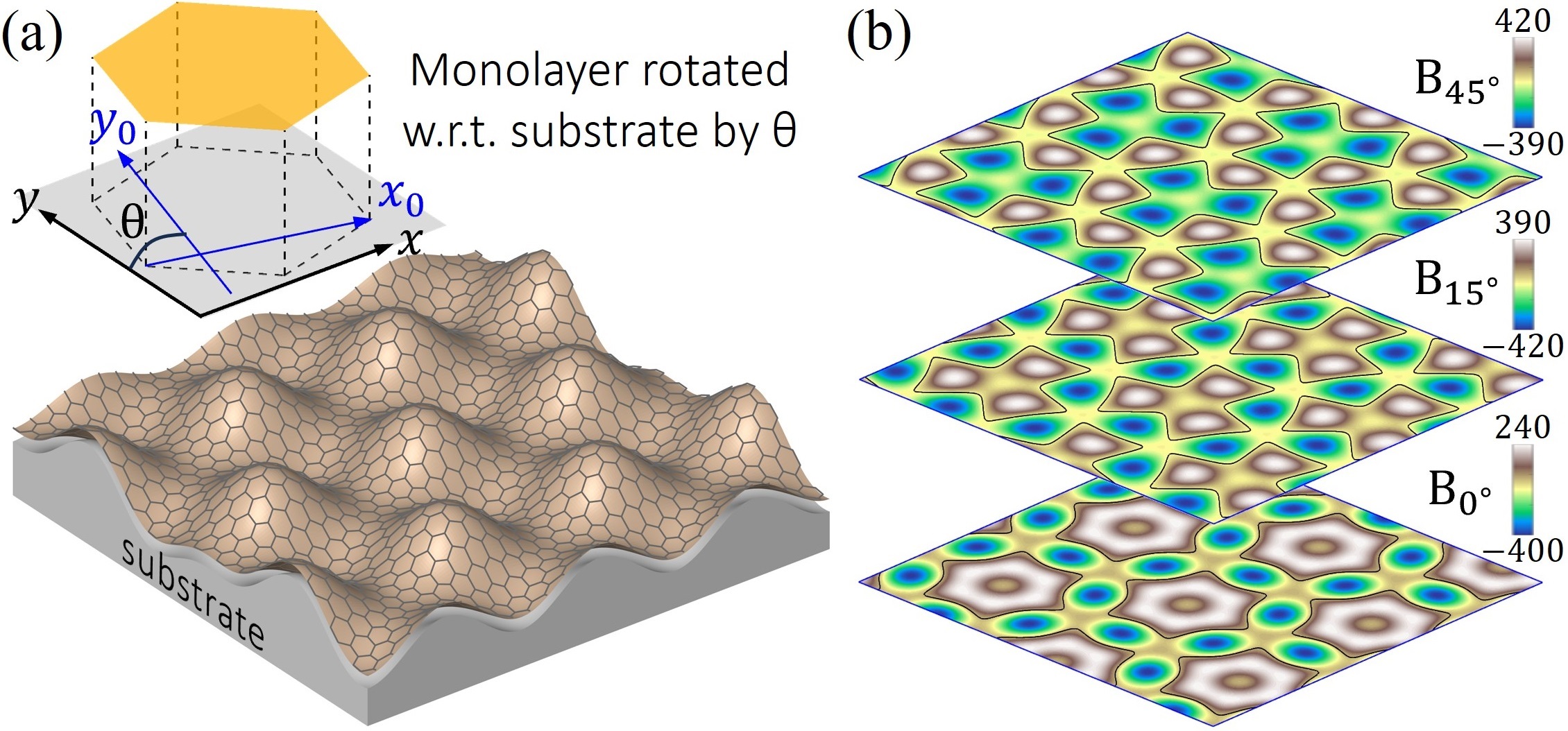
Figure 4: (a) Schematics of a honeycomb lattice on a patterned substrate, whose zigzag/armchair crystalline directions ($x_{0}/y_{0}$ axis in the inset) are rotated clockwise by $\theta$ degrees from the $x/y$ axis on the substrate. The inset shows the $\theta$ rotation of the $x_{0}y_{0}$ coordinate frame on the lattice (yellow hexagon) with respect to the $xy$ coordinate frame on the substrate (grey square). (b) Pseudo-magnetic field (units: T) $B_{\theta}$ in the $+K$ valley for different $\theta$ with black curves denoting zero-field contours. Parameters: $h_{0}=0.6$ nm, $L=14$ nm, and $\Delta=0.825$ eV, $\hbar v=3.38$ eV$\cdot$Å, $evA_{0}=2$ eV from WSe₂.

Crucially, the strain distribution on the lattice and the resultant pseudo-magnetic field depend on the alignment between the lattice and substrate. This is understandable as the local atomic bonds on the lattice are stressed differently when the alignment is varied, although the macroscopic topography of the membrane remains invariant [see e.g., Fig. 5(a)]. This feature underlies the twist-control of the pseudo-magnetic field by rotating the material with respect to the substrate.

To elaborate on this twist control of pseudo-magnetic field, we notice that there are two coordinate frames that are of interest [see Fig. 4(a)]: (i) $xy$, fixed on the substrate, in which $z(\boldsymbol{r})$ is defined; (ii) $x_{0}y_{0}$, fixed on lattice, with $x_{0}$ ($y_{0}$) along its zigzag (armchair) direction. The angle $\theta$ between the $x_{0}$ ($y_{0}$) and $x$ ($y$) axes characterizes the alignment of the lattice with respect to the substrate. Without loss of generality, we assume that the lattice is rotated clockwise with respect to the substrate by $\theta$ degrees. Here it is convenient to use the $xy$ coordinate frame fixed on the substrate, in which expressions of the out-of-plane deformation $z(\boldsymbol{r})$ and the strain tensor components $\epsilon_{ij}$ remain independent of $\theta$. In this coordinate frame, the effect of twisting is manifested in the strain vector potential, which gains an explicit $\theta$-dependence Jiang et al. (2013); Zhai and Sandler (2018):

$$\boldsymbol{A}_{\theta}=R(3\theta)A_{0}(\epsilon_{xx}-\epsilon_{yy},\,-2\epsilon_{xy})^{T}.~{}$$ (20)

Here $R(3\theta)$ is the clockwise rotation matrix by $3\theta$ degrees and $A_{0}$ is a material-dependent constant (see Sec. S2 of Supplementary Material sup ). When $\theta=0^{\circ}$, the strain vector potential reads $\boldsymbol{A}_{0^{\circ}}=A_{0}(\epsilon_{xx}-\epsilon_{yy},-2\epsilon_{xy})^{T}$, which is commonly found in the literature as the zigzag direction is usually implicitly chosen as the $x$ axis Vozmediano et al. (2010); Amorim et al. (2016); Naumis et al. (2017). The twist control of the pseudo-magnetic field by rotating the lattice on the substrate is explicitly manifested in its $\theta$-dependence, $\tau\boldsymbol{B}_{\theta}=\nabla\times(\tau\boldsymbol{A}_{\theta})$. Figure 4(b) shows $\boldsymbol{B}_{\theta}$ in the $xy$ coordinate frame in the $\tau=+$ valley for a few different $\theta$. One can see that both the magnitude and profile of the field change with $\theta$. In particular, one notices that $\boldsymbol{B}_{15^{\circ}}$ and $\boldsymbol{B}_{45^{\circ}}$ are effectively opposite (up to a rotation), which we will employ in the following.

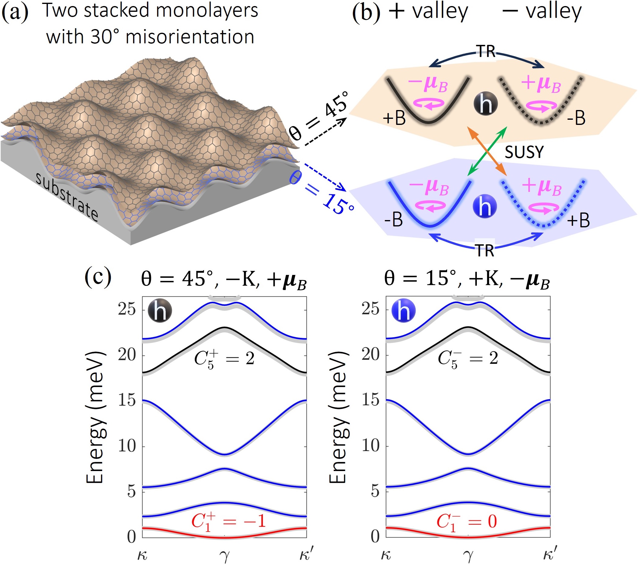
Figure 5: (a) Schematics of two $30^{\circ}$ misorientated honeycomb lattices on a patterned substrate, whose zigzag/armchair crystalline directions are rotated clockwise from the $x/y$ axis on the substrate by $\theta=15^{\circ}$ and $45^{\circ}$, respectively. The corresponding pseudo-magnetic field $B_{\theta}$ in the $+K$ valley are shown in Fig. 4(b). (b) Schematics of Dirac cones (solid/dotted: $+K$/$-K$) and valley magnetic moments (curly arrows) for holes in the two $30^{\circ}$ misorientated layers (hexagon backgrounds). $\pm B$ in each column highlight the opposite pseudo-magnetic fields in the two layers. (c) Energy bands of holes and Chern numbers for the case of $\{\theta=45^{\circ},\,-K\text{ valley}\}$ vs $\{\theta=15^{\circ},\,+K\text{ valley}\}$. All the blue bands have zero Chern numbers. Grey curves in the background represent results from the Dirac model [Eq. (17)]. Parameters: $h_{0}=0.6$ nm, $L=14$ nm, and $\Delta=0.825$ eV, $\hbar v=3.38$ eV$\cdot$Å, $evA_{0}=2$ eV from WSe₂.

IV.1.3 Isospectral bands with layer contrasted topology

We note that stacked monolayers with $\sim 30^{\circ}$ misorientation are decoupled at low energies due to the large momentum separation of the band edges in the two layers Piccinini et al. (2021). Therefore, by depositing two layers of TMDs with $\theta=15^{\circ}$ and $\theta=45^{\circ}$ respectively on the substrate [Fig. 5(a)], one can achieve two decoupled layers with layer-opposite pseudo-magnetic fields [see Fig. 4(b)]. In such a bilayer configuration, holes in opposite layers and opposite valleys are governed by Eq (19), thus behave as SPs [Fig. 5(b)]. As there are two valleys in each layer, which are related by time-reversal (TR) symmetry, this configuration contains two sets of TR partners as well as two sets of SPs.

Figure 5(c) presents the identical energy spectra for such SPs by considering two layers of WSe₂ stacked on the substrate as described above. As the $\pm$ valleys are connected by TR symmetry, only the bands from one valley in each layer are shown. The colored curves represent results from the hole model [Eq. (18)], which match perfectly with the grey curves from the Dirac model [Eq. (17)] shown in the background com (d). The first bands of the SPs exhibit distinct band Chern numbers $C_{1}^{+}=-1$ vs $C_{1}^{-}=0$. They satisfy $C_{1}^{-}-C_{1}^{+}=1$, which is expected for a quadratic band dispersion around $\gamma$ –location of the zero mode– as dictated by Eq. (15) (also see Fig. 2).

One might also notice that the first bands of strained TMDs in Fig. 5(c) are much narrower than their counterparts in graphene Milovanović et al. (2020); Manesco et al. (2021); Manesco and Lado (2021); Phong and Mele (2022); Mahmud et al. (2023); Gao et al. (2023). Hence they might be alternative candidates for exploring correlation-driven phenomena, such as the fractional Chern insulating phases in the topologically nontrivial band Gao et al. (2023); Park et al. (2023); Cai et al. (2023); Anderson et al. (2023); Zeng et al. (2023); Xu et al. (2023); Li et al. (2021); Wang et al. (2024); Reddy et al. (2023); Yu et al. (2024) and other interesting features Dong et al. (2023); Goldman et al. (2023); Fan et al. (2024); Liu et al. (2023).

IV.2 $30^{\circ}$ twisted double bilayer TMDs for $N=2$ SUSY with quartic dispersion

In this section, we propose a physical system for the scenario of $N=2$ SUSY in Eq. (7). It allows us to obtain $C_{1}^{-}-C_{1}^{+}=2$ thanks to the quartic dispersion around the zero mode [Fig. 2(a)]. Such cases are useful for achieving topological bands with higher Chern numbers. The system is realized with the replacement of each monolayer in Fig. 5(a) by a bilayer, as shown schematically in Fig. 6(a). Notably, the isospectral SPs realized are still in stark contrast to the time-reversal partners, with one SP being topologically trivial ($C_{1}^{-}=0$), and another nontrivial ($C_{1}^{+}=-2$).

We first look at the basic ingredient of the setup– a strained bilayer. For illustrative purposes, it suffices to consider a simple bilayer Hamiltonian

$$\mathcal{H}_{\tau}^{\text{2L}}=\begin{pmatrix}H_{\tau}^{\text{D}}&T\\ T^{\dagger}&H_{\tau}^{\text{D}}\end{pmatrix}~{}\text{ with }~{}T=\begin{pmatrix}0&0\\ t&0\end{pmatrix},$$ (21)

where $H_{\tau}^{\text{D}}=v\boldsymbol{\sigma}_{\tau}\cdot(\boldsymbol{p}+\tau e\boldsymbol{A})+\Delta\sigma_{z}$ is the Dirac Hamiltonian for a strained monolayer, and $t$ is the interlayer coupling constant. This simple model can describe rhombohedral bilayer TMDs Zhang et al. (2018b); Tong et al. (2017), where $t\sim 0.1$ eV from a recent experiment Liang et al. (2022). By focusing on holes, one can consider a low-energy model

$$\mathcal{H}_{\tau}^{h}\psi=\frac{v^{4}}{2\Delta t^{2}}(\tau\pi_{x}^{\tau}+i\pi_{y}^{\tau})^{2}(\tau\pi_{x}^{\tau}-i\pi_{y}^{\tau})^{2}\psi=\varepsilon\psi,$$ (22)

where $(\pi_{x}^{\tau},\,\pi_{y}^{\tau})=\boldsymbol{\pi}^{\tau}=\boldsymbol{p}+\tau e\boldsymbol{A}$. This equation is valid for $\varepsilon\ll t,\,\Delta$. One may notice that $\mathcal{H}_{\tau}^{h}$ can also describe holes in Bernal bilayer graphene by introducing an interlayer displacement field into the two-band model McCann and Koshino (2013). In this case, $\Delta$ is replaced by the displacement field, and $t\sim 0.4$ eV. The Hamiltonian $\mathcal{H}_{\tau}^{h}$ resembles that in Eq. (7) with $N=2$, thus lays the basis for constructing the SUSY model.

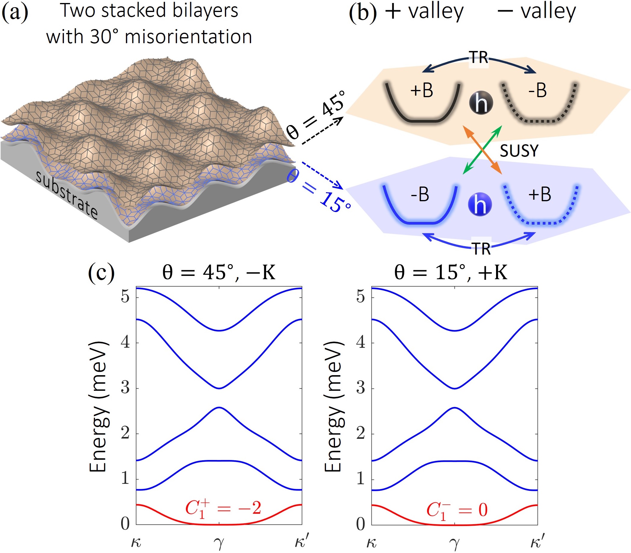
Figure 6: (a) Schematics of two $30^{\circ}$ misorientated rhombohedral bilayer TMDs on a patterned substrate, whose zigzag/armchair crystalline directions are rotated clockwise from the $x/y$ axis on the substrate by $\theta=15^{\circ}$ and $45^{\circ}$, respectively. The corresponding strain pseudo-magnetic field in the $+K$ valley are shown in Fig. 4(b). (b) Schematics of quartic cones (solid/dotted: $+K$/$-K$) for holes in the two $30^{\circ}$ misorientated bilayers (hexagon backgrounds). $\pm B$ in each column highlight the opposite pseudo-magnetic fields in the two layers. (c) Energy bands of holes for the case of $\{\theta=45^{\circ},\,-K\text{ valley}\}$ vs $\{\theta=15^{\circ},\,+K\text{ valley}\}$. All the blue bands have zero Chern numbers. Parameters: $h_{0}=0.6$ nm, $L=14$ nm, $t=0.1$ eV, and $\Delta=0.825$ eV, $\hbar v=3.38$ eV$\cdot$Å, $evA_{0}=2$ eV from WSe₂.

By following a similar idea as in Fig. 5(a), the SUSY model in Eq. (7) with $N=2$ can be realized by using two copies of bilayer TMDs with layer-opposite strain pseudo-magnetic fields (i.e., $\boldsymbol{B}^{(1)}=-\boldsymbol{B}^{(2)}$). Then holes from opposite valleys of opposite bilayers form SPs, for example,

$$\begin{aligned} \mathcal{H}_{\tau=+}^{h}(\text{bilayer}~{}1)&=\frac{v^{4}}{2\Delta t^{2}}[\pi_{+}(\boldsymbol{A}^{(1)})]^{2}[\pi_{-}(\boldsymbol{A}^{(1)})]^{2}\\ \mathcal{H}_{\tau=-}^{h}(\text{bilayer}~{}2)&=\frac{v^{4}}{2\Delta t^{2}}[\pi_{-}(\boldsymbol{A}^{(1)})]^{2}[\pi_{+}(\boldsymbol{A}^{(1)})]^{2}\end{aligned},~{}$$ (23)

where the notation $\pi_{\pm}(\boldsymbol{A}^{(1)})=(p_{x}+eA_{x}^{(1)})\pm i(p_{y}+eA_{y}^{(1)})$ has been used, and $-\boldsymbol{A}^{(2)}$ has been replaced by $\boldsymbol{A}^{(1)}$ in layer 2. It now becomes clear that they correspond to $\mathbb{H}_{\mp}$ in Eq. (7) with $N=2$. In this form it is also evident that the low-energy dispersion will be quartic, thus one expects $C_{1}^{-}-C_{1}^{+}=2$ if there is one zero mode on the first band [Fig. 2(a)].

By depositing double bilayers with $\theta=15^{\circ}$ and $\theta=45^{\circ}$ respectively on the substrate [Fig. 6(a)], opposite pseudo-magnetic fields in the two bilayers can be achieved [see Fig. 4(b)], thus realizing the model of Eq. (23). Figure 6(c) shows representative energy bands for such SPs by considering double bilayers of WSe₂. The low-energy bands are obtained from Eq. (21) due to its simplicity. The band structure around the zero mode at $\gamma$ clearly shows a quartic dispersion [also compare with Fig. 5(c)]. The first bands of the SPs exhibit distinct band topology characterized by $C_{1}^{+}=-2$ vs $C_{1}^{-}=0$, which is consistent with $C_{1}^{-}-C_{1}^{+}=2$ due to the quartic dispersion around $\gamma$ [Eq. (15) and Fig. 2(a)].

V SUSY dictated topology in square-root Hamiltonian and manifestions in flat-band superlattices

We note that many 2D superlattice models that exhibit exact flat bands at magic angles, e.g., twisted bilayer graphene (TBG) in the chiral limit Tarnopolsky et al. (2019) and the strained $\Gamma$-valley model with quadratic band touching Wan et al. (2023a), as well as the square-root topological materials Arkinstall et al. (2017); Ezawa (2020); Mizoguchi et al. (2020); Yoshida et al. (2021), are described by Hamiltonian that can be considered as the ‘square root’ of $\mathcal{H}_{\text{susy}}$ in Eq. (1). Here we show that such square-root Hamiltonian, $H_{\text{sqrt}}$, as defined below in Eq. (24), exhibits intriguing electronic and topological properties that can be traced back to the SUSY systems. In particular, the isospectra of SPs underlies a symmetric spectrum of $H_{\text{sqrt}}$, i.e., $E^{\text{sqrt}}_{\boldsymbol{k}}\leftrightarrow-E^{\text{sqrt}}_{\boldsymbol{k}}$, while the contrasted topologies of SPs, i.e., $C_{1}^{+}\neq C_{1}^{-}$, are inherited by the first conduction and valence bands of $H_{\text{sqrt}}$. The SUSY formalism discussed in earlier sections therefore connects many seemingly different systems and underlies the emergence of contrasted band topology.

V.1 Linking electronic and topological properties of $H_{\text{sqrt}}$ to $\mathcal{H}_{\text{susy}}$

Here we define the square root of $\mathcal{H}_{\text{susy}}$ in Eq. (1) as

$$H_{\text{sqrt}}=\begin{pmatrix}\Delta\mathbb{I}&M\\ M^{\dagger}&-\Delta\mathbb{I}\end{pmatrix},$$ (24)

where $\Delta$ is a constant and $\mathbb{I}$ is the identity matrix com (e). In the following we will assume $\Delta\geq 0$, and the discussions are general, not limited to the forms of $M$ in Eq. (6). $H_{\text{sqrt}}$ can be considered as the square root of $\mathcal{H}_{\text{susy}}$ in the sense that its square yields $\mathcal{H}_{\text{susy}}$ up to a constant:

$$H_{\text{sqrt}}^{2}=\begin{pmatrix}MM^{\dagger}&0\\ 0&M^{\dagger}M\end{pmatrix}+\Delta^{2}=\mathcal{H}_{\text{susy}}+\Delta^{2},$$ (25)

where the identity matrix has been removed for simplicity. As the SP Hamiltonian $\mathbb{H}_{+}=MM^{\dagger}$ and $\mathbb{H}_{-}=M^{\dagger}M$ have identical positive energies, which will be denoted as $\mathcal{E}>0$, Eq. (25) dictates that the spectrum of $H_{\text{sqrt}}$ consists of $E^{\text{sqrt}}=\sqrt{\mathcal{E}+\Delta^{2}}>\Delta$, $E^{\text{sqrt}}=-\sqrt{\mathcal{E}+\Delta^{2}}<-\Delta$, and $E^{\text{sqrt}}=\pm\Delta$ if $\mathbb{H}_{\pm}$ have zero modes. This points to a symmetric spectrum for $H_{\text{sqrt}}$ with the possible exception at energies $\pm\Delta$, where the eigenmodes are also dubbed as threshold modes.

When $\Delta=0$, the square-root Hamiltonian $H_{\text{sqrt}}$ has chiral symmetry, i.e., it satisfies $\{H_{\text{sqrt}},\,\Sigma_{z}\}=0$ with $\Sigma_{z}=\text{diag}(\mathbb{I},\,-\mathbb{I})$. Many lattice models consider such a case Ezawa (2020); Mizoguchi et al. (2020); Yoshida et al. (2021); Roychowdhury et al. (2022). Chiral symmetry ensures a symmetric spectrum $E\leftrightarrow-E$, however, it should be noted that symmetric spectrum can also appear from SUSY in the absence of chiral symmetry when $\Delta\neq 0$.

When $\Delta\neq 0$, the relation $\{H_{\text{sqrt}},\,[H_{\text{sqrt}},\,\Sigma_{z}]\}=0$ is satisfied, thus $[H_{\text{sqrt}},\,\Sigma_{z}]\propto Q^{\dagger}-Q$ [see Eq. (3)] transforms eigenstates of $H_{\text{sqrt}}$ with opposite energies into each other Kailasvuori (2009). An exception occurs for the threshold modes: $Q$ and $Q^{\dagger}$ annihilate the threshold modes, $\Psi_{\Delta}^{\text{sqrt}}=(\psi_{+}^{0},\,0)^{T}$ and $\Psi_{-\Delta}^{\text{sqrt}}=(0,\,\psi_{-}^{0})^{T}$, which are also the zero modes of $\mathcal{H}_{\text{susy}}$ satisfying $M^{\dagger}\psi_{+}^{0}=0$ and $M\psi_{-}^{0}=0$. Thus the energy levels at $E^{\text{sqrt}}=\Delta$ and $E^{\text{sqrt}}=-\Delta$ are not necessarily paired. However, intriguing features can emerge when $H_{\text{sqrt}}$ has symmetric threshold modes at both $\Delta$ and $-\Delta$, or equivalently, when $\mathbb{H}_{+}$ and $\mathbb{H}_{-}$ both have zero modes, which will be the focus now.

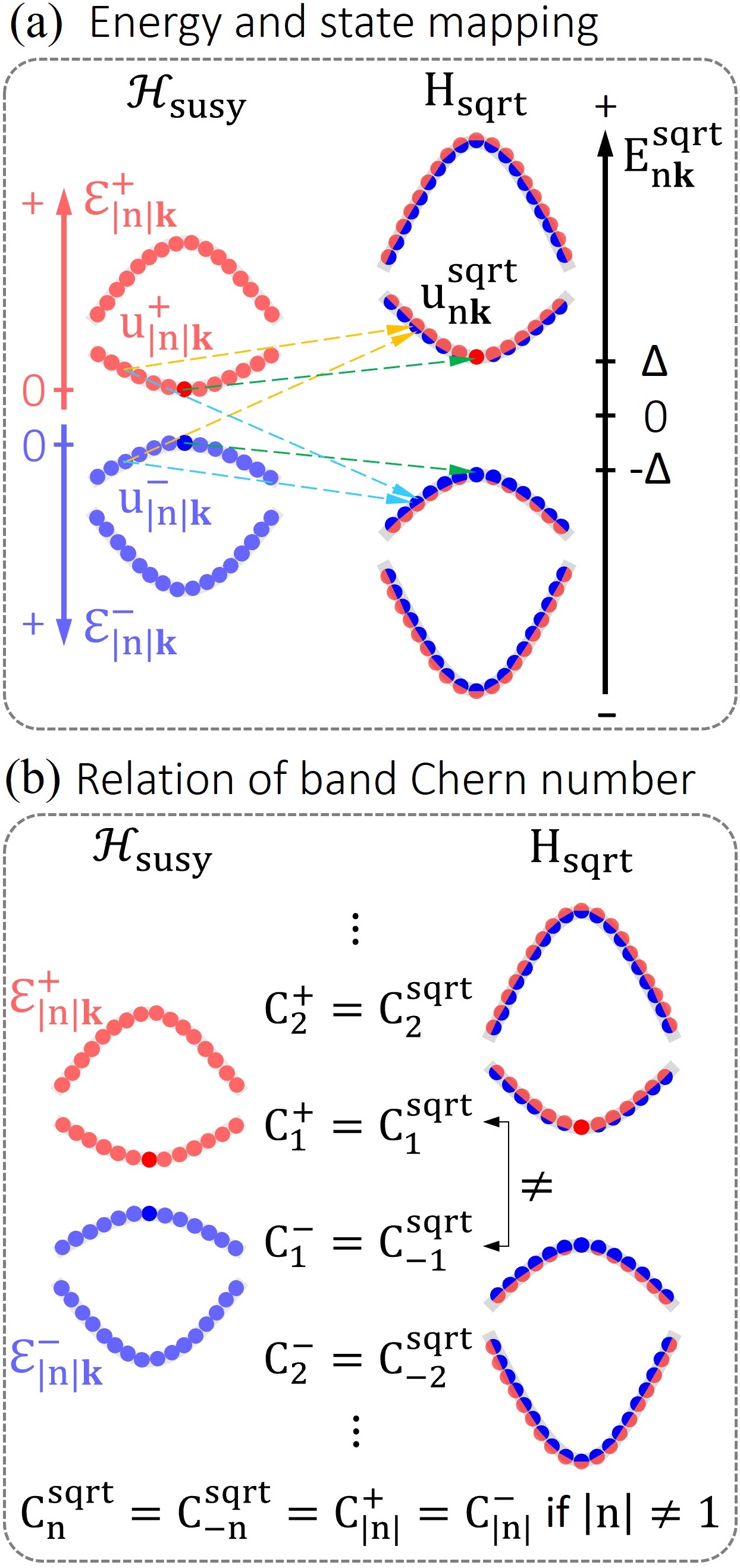
Figure 7: (a) Schematics of mapping from energy $\mathcal{E}_{|n|\boldsymbol{k}}^{\pm}$ and states $u_{|n|\boldsymbol{k}}^{\pm}$ of $\mathbb{H}_{\pm}$ to those of $H_{\text{sqrt}}$. The energies are mapped into each other via $E_{n\boldsymbol{k}}^{\text{sqrt}}=\pm(\mathcal{E}_{|n|\boldsymbol{k}}^{\pm}+\Delta^{2})^{1/2}$. The ${E}_{n\boldsymbol{k}}^{\text{sqrt}}$ dispersions on the right column consist of dots whose red and blue portions represent the $u_{|n|\boldsymbol{k}}^{+}$ and $u_{|n|\boldsymbol{k}}^{-}$ components of $u_{n\boldsymbol{k}}^{\text{sqrt}}$ respectively [see Eq. (27)]. The zero modes of $\mathbb{H}_{+}$ ($\mathbb{H}_{-}$) are exactly mapped to the threshold modes of $H_{\text{sqrt}}$ at energies $+\Delta$ ($-\Delta$). Other states of $H_{\text{sqrt}}$ involve a mixture of $u_{|n|\boldsymbol{k}}^{+}$ and $u_{|n|\boldsymbol{k}}^{-}$. (b) Relation of band Chern numbers of $H_{\text{sqrt}}$ (denoted as $C_{n}^{\text{sqrt}}$) to those of $\mathbb{H}_{\pm}$ (denoted as $C_{|n|}^{\pm}$).

In the following we consider periodic systems. Bloch functions of the periodic $H_{\text{sqrt}}$ are also related to those of $\mathbb{H}_{\pm}$. We denote the eigenvalue of the Bloch Hamiltonian $H_{\text{sqrt}}(\boldsymbol{k})$ as $E_{n\boldsymbol{k}}^{\text{sqrt}}$, with $n=\pm 1,\pm 2,\cdots$ labeling conduction ($n>0$) and valence ($n<0$) bands in ascending order of energy magnitude. The eigenvalues of $\mathbb{H}_{\pm}(\boldsymbol{k})$, which are non-negative, will be denoted as $\mathcal{E}_{|n|\boldsymbol{k}}^{\pm}$ with $|n|=1,2,\cdots$, and they satisfy

$$\mathcal{E}_{|n|\boldsymbol{k}}^{\pm}=\left(E_{n\boldsymbol{k}}^{\text{sqrt}}\right)^{2}-\Delta^{2}\geq 0.$$ (26)

Given the SP Bloch states $u_{|n|\boldsymbol{k}}^{\pm}$ satisfying $\mathbb{H}_{\pm}(\boldsymbol{k})u_{|n|\boldsymbol{k}}^{\pm}=\mathcal{E}_{|n|\boldsymbol{k}}^{\pm}u_{|n|\boldsymbol{k}}^{\pm}$, one can obtain the normalized Bloch state of $H_{\text{sqrt}}(\boldsymbol{k})$ in terms of $u_{|n|\boldsymbol{k}}^{\pm}$ as

$$u_{n\boldsymbol{k}}^{\text{sqrt}}\equiv\begin{pmatrix}c_{n\boldsymbol{k}}^{+}u_{|n|\boldsymbol{k}}^{+}\\ c_{n\boldsymbol{k}}^{-}u_{|n|\boldsymbol{k}}^{-}\end{pmatrix}=\begin{pmatrix}\sqrt{\frac{E_{n\boldsymbol{k}}^{\text{sqrt}}+\Delta}{2E_{n\boldsymbol{k}}^{\text{sqrt}}}}u_{|n|\boldsymbol{k}}^{+}\\ \text{sgn}(E_{n\boldsymbol{k}}^{\text{sqrt}})\sqrt{\frac{E_{n\boldsymbol{k}}^{\text{sqrt}}-\Delta}{2E_{n\boldsymbol{k}}^{\text{sqrt}}}}u_{|n|\boldsymbol{k}}^{-}\end{pmatrix}.$$ (27)

In general, the two-component $u_{n\boldsymbol{k}}^{\text{sqrt}}$ consists of both SP Bloch functions $u_{|n|\boldsymbol{k}}^{\pm}$, except for the threshold modes at energy $E_{n\boldsymbol{k}}^{\text{sqrt}}=\Delta$ ($-\Delta$), which are fully polarized on $u_{|n|\boldsymbol{k}}^{+}$ ($u_{|n|\boldsymbol{k}}^{-}$) that correspond to the zero modes of $\mathbb{H}_{+}$ ($\mathbb{H}_{-}$).

When the bands are narrow, satisfying $|E_{n\boldsymbol{k}}^{\text{sqrt}}|-\Delta\ll\Delta$, one finds $c_{n\boldsymbol{k}}^{+}\approx 1$ & $c_{n\boldsymbol{k}}^{-}\approx 0$ ($c_{n\boldsymbol{k}}^{+}\approx 0$ & $c_{n\boldsymbol{k}}^{-}\approx-1$) in the conduction (valence) bands, thus $u_{n\boldsymbol{k}}^{\text{sqrt}}$ is near fully polarized on the $u_{|n|\boldsymbol{k}}^{+}$ ($u_{|n|\boldsymbol{k}}^{-}$) component. In such cases, electrons in the conduction and valence bands of $H_{\text{sqrt}}$ can be well described by $H_{\text{sqrt}}^{c}=MM^{\dagger}/(2\Delta)$ and $H_{\text{sqrt}}^{v}=-M^{\dagger}M/(2\Delta)$, respectively.

The mapping from energy $\mathcal{E}_{|n|\boldsymbol{k}}^{\pm}$ and states $u_{|n|\boldsymbol{k}}^{\pm}$ of $\mathbb{H}_{\pm}$ to those of $H_{\text{sqrt}}$ are shown schematically in Fig. 7(a). In the right column, the ${E}_{n\boldsymbol{k}}^{\text{sqrt}}$ dispersions consist of dots whose red and blue portions represent the $u_{|n|\boldsymbol{k}}^{+}$ and $u_{|n|\boldsymbol{k}}^{-}$ components of $u_{n\boldsymbol{k}}^{\text{sqrt}}$ respectively [see Eq. (27)]. Reciprocally, one can deduce the eigenenergies and eigenstates of $\mathbb{H}_{\pm}$ from $E_{n\boldsymbol{k}}^{\text{sqrt}}$ and $u_{n\boldsymbol{k}}^{\text{sqrt}}$. And usually diagonalizing $H_{\text{sqrt}}$ can be done more conveniently as $H_{\text{sqrt}}$ is linear in $M$ and $M^{\dagger}$.

Eq. (27) further implies that the band topology of $H_{\text{sqrt}}$ are related to those of $\mathbb{H}_{\pm}$. Recall that the states $u_{|n|\boldsymbol{k}}^{\pm}$ are paired by Eq. (5) when the energy is nonzero, this allows one to relate the Berry connection of $H_{\text{sqrt}}$ to those of $\mathbb{H}_{\pm}$, whose details are given in Sec. S4 of Supplementary Material sup . From such relations, we arrive at the following connections between the band Chern numbers of $H_{\text{sqrt}}$ (denoted as $C_{n}^{\text{sqrt}}$) and those of $\mathbb{H}_{\pm}$ (denoted as $C_{|n|}^{\pm}$):

$$C_{n}^{\text{sqrt}}=\begin{cases}C_{|n|}^{+}=C_{|n|}^{-}&\text{if $|n|>1$}\\ C_{1}^{+}&\text{if $n=1$}\\ C_{1}^{-}&\text{if $n=-1$}\end{cases}.$$ (28)

These relations, schematically summarized in Fig. 7(b), are rather generic and not limited to the forms of $M$ in Eq. (6) and value of $\Delta$. Therefore, the symmetric energy bands of $H_{\text{sqrt}}$ are accompanied by symmetric Chern numbers, i.e. $C_{n}^{\text{sqrt}}=C_{-n}^{\text{sqrt}}$, except for the first conduction ($n=1$) and valence ($n=-1$) bands that contain the threshold modes.

Incidentally, in the case of $\Delta=0$, one readily notices that chiral symmetry also underlies the identical Chern numbers between the $|n|>1$ conduction and valence bands, but in the generic case this equality relation is traced back to Eq. (12)– a consequence of SUSY. And with the chiral symmetry at $\Delta=0$, topology of the square-root Hamiltonian is also noted in some lattice models Arkinstall et al. (2017); Ezawa (2020); Mizoguchi et al. (2020); Yoshida et al. (2021).

When chiral symmetry is broken in the case of $\Delta\neq 0$, our findings give insights on how contrasted topology of conduction and valence bands arises from the SUSY of the squared Hamiltonian, as dictated by the zero modes and the dispersion in their vicinity in the SUSY spectrum (e.g., Fig. 2). With $\Delta>0$, the Chern numbers are well defined in the first conduction and valence bands of $H_{\text{sqrt}}$, and $C_{1}^{\text{sqrt}}=C_{1}^{+}$ and $C_{-1}^{\text{sqrt}}=C_{1}^{-}$ are satisfied. So $C_{1}^{\text{sqrt}}\neq C_{-1}^{\text{sqrt}}$ when the dispersion in the vicinity of threshold/zero mode determines a finite difference between $C_{1}^{+}$ and $C_{1}^{-}$ [see e.g., Eq. (15) and Fig. 2]. The contrasted topology of the SPs of the squared Hamiltonian in bands containing their zero modes are therefore transferred to the first conduction and valence bands of $H_{\text{sqrt}}$ respectively [Fig. 7(b)].

V.2 Manifestions in flat-band superlattices

Figure S3 in the Supplementary Material sup confirms the above results with a simple example of $H_{\text{sqrt}}$ that describes massive Dirac fermions in a periodic magnetic field [see Fig. 1(a)]. Specifically, here $M=\pi_{-}$, and the associated SUSY system $\mathbb{H}_{\pm}$ are given by Eq. (9). By comparing Fig. S3(b) and Fig. 1(b), we find $C_{1}^{\text{sqrt}}=-1=C_{1}^{+}$ vs $C_{-1}^{\text{sqrt}}=0=C_{1}^{-}$, and $C_{n}^{\text{sqrt}}=C_{-n}^{\text{sqrt}}=C_{|n|}^{+}=C_{|n|}^{-}$ otherwise, which is consistent with Eq. (28) and Fig. 7(b). This model of $H_{\text{sqrt}}$, and its TR counterpart, can be realized by using strained graphene with a staggered potential Mahmud et al. (2023); Phong and Mele (2022); Wan et al. (2023b); Gao et al. (2023).

TBG in the chiral limit Tarnopolsky et al. (2019) and strained bilayer graphene (SBG) Wan et al. (2023b) are another two important examples where the contrasted topology of the conduction and valence minibands containing the threshold modes are dictated by Eqs. (15) and (16). On one hand, they serve as cases with non-Abelian gauge fields San-Jose et al. (2012), on the other hand, they both exhibit $C_{-1}^{\text{sqrt}}-C_{1}^{\text{sqrt}}=2$, but due to drastically different origins. They both can be formulated in the form of $H_{\text{sqrt}}=\sigma_{x}\otimes(p_{x}+e\mathcal{A}_{x})+\sigma_{y}\otimes(p_{y}+e\mathcal{A}_{y})$, as detailed in Supplementary Material sup . Unlike a usual magnetic field, here $\boldsymbol{\mathcal{A}}=(\mathcal{A}_{x},\,\mathcal{A}_{y})$ is a non-Abelian gauge potential due to interlayer coupling, and the associated non-Abelian gauge field reads $\boldsymbol{\mathcal{B}}=\nabla\times\boldsymbol{\mathcal{A}}+i\frac{e}{\hbar}[\mathcal{A}_{x},\,\mathcal{A}_{y}]\hat{\boldsymbol{z}}$. They are matrices due to the layer degree of freedom in a hybridized bilayer. The associated SUSY Hamiltonian is given by the square of $H_{\text{sqrt}}$, i.e., $\mathbb{H}_{\pm}=\frac{1}{2m}(\boldsymbol{p}+e\boldsymbol{\mathcal{A}})^{2}\pm\boldsymbol{\mu}_{B}\cdot\boldsymbol{\mathcal{B}}$. The results discussed earlier, e.g., contrasted band topology in $\mathbb{H}_{\pm}$, thus can be applied directly. Let us focus on band topology and highlight the similarity/difference between TBG and SBG. In TBG, one expects $C_{1}^{-}-C_{1}^{+}=2$ because each SP has two zero modes (at the Dirac points, and we assume the twist angle is not magic Bistritzer and MacDonald (2011); Tarnopolsky et al. (2019)), around which the low-energy dispersion of $\mathbb{H}_{\pm}$ is quadratic [see Fig. 2(b)]. While $C_{1}^{-}-C_{1}^{+}=2$ is also expected in SBG, it instead results from one zero mode for each SP with quartic dispersion. If a sublattice staggered potential is added to introduce a finite $\Delta$ in $H_{\text{sqrt}}$, these results will manifest in the conduction and valence bands of $H_{\text{sqrt}}$ as $C_{-1}^{\text{sqrt}}-C_{+1}^{\text{sqrt}}=2$, which are consistent with numerical results (see Fig. S4(c) and Fig. S5(b) of Supplementary Material sup ).

The strained $\Gamma$-valley model with quadratic band touching Wan et al. (2023a) is an example that differs from all previous examples. Its Hamiltonian also has the form of $H_{\text{sqrt}}$, whereas $M=(p_{x}^{2}-p_{y}^{2}+f_{1})-i(2p_{x}p_{y}+f_{2})$ with $f_{1,2}(\boldsymbol{r})$ being some space-dependent functions, thus the effects of strain cannot be understood in terms of a gauge field. Nevertheless, topological flat bands and magic angles –like those in TBG– are also discovered. Our results show that its band topology are inherited from the associated $\mathcal{H}_{\text{susy}}$, thus provide insights for understanding the emergence of nontrivial topology and the distinct Chern numbers in the bands that contain the zero/threshold modes.

VI Summary and discussions

In this work, we focus on SUSY systems that involve electrons in a zero-flux gauge field. We reveal that the SPs have isospectra, yet remarkably, the energy bands that contain the zero modes exhibit distinct topology [e.g., Fig. 1(b)]: the difference in their Chern numbers is determined by the number of zero modes and low-energy dispersion around them (Fig. 2). This puts forward a new scenario of band degeneracy, where the two degenerate partners can be topologically trivial and nontrivial respectively, in stark contrast to the scenario due to the time-reversal symmetry. Such SUSY models can be realized in multilayer 2D semiconductors by twist and strain engineering (e.g., Figs. 5 and 6). We also generalize the discussions to systems whose physical Hamiltonian corresponds to the square root of a SUSY Hamiltonian, where the topological properties of the two SUSY SPs are transferred to the conduction and valence bands of the physical Hamiltonian respectively (Fig. 7). As many of the flat-band systems are described by such square-root models, our findings offer a unifying picture to understand their topological properties. It is conceivable that the knowledge of various SUSY systems and the zero modes Junker (2019) will introduce novel insights and platforms for exploring the correlation-driven phenomena that are actively pursued in superlattice materials recently.

Finally, we note that extra terms that break SUSY often exist in some of the discussed systems. For example, the model of TBG in the nonchiral limit contains an effective scalar potential San-Jose et al. (2012). However, provided such terms are not prominent, SUSY will only be weakly broken, thus the SUSY dictated topological properties are expected to remain unaffected in the nearly symmetric spectra. This is clearly manifested in TBG, in which the energy spectrum remain approximately symmetric at different twist angles Moon and Koshino (2013) with SUSY dictated Chern numbers for the first conduction/valence bands.

VII Acknowledgment

We thank Nancy Sandler, Bo Fu, and Ci Li for helpful discussions. The work is supported by Research Grant Council of Hong Kong SAR China (HKU SRFS2122-7S05 and AoE/P-701/20), and New Cornerstone Science Foundation.

References

- Cao et al. (2018a) Y. Cao, V. Fatemi, S. Fang, K. Watanabe, T. Taniguchi, E. Kaxiras, and P. Jarillo-Herrero, Nature 556, 43 (2018a).
- Cao et al. (2018b) Y. Cao, V. Fatemi, A. Demir, S. Fang, S. L. Tomarken, J. Y. Luo, J. D. Sanchez-Yamagishi, K. Watanabe, T. Taniguchi, E. Kaxiras, R. C. Ashoori, and P. Jarillo-Herrero, Nature 556, 80 (2018b).
- Andrei and MacDonald (2020) E. Y. Andrei and A. H. MacDonald, Nat. Mater. 19, 1265 (2020).
- Balents et al. (2020) L. Balents, C. R. Dean, D. K. Efetov, and A. F. Young, Nat. Phys. 16, 725 (2020).
- Kennes et al. (2021) D. M. Kennes, M. Claassen, L. Xian, A. Georges, A. J. Millis, J. Hone, C. R. Dean, D. N. Basov, A. N. Pasupathy, and A. Rubio, Nat. Phys. 17, 155 (2021).
- Andrei et al. (2021) E. Y. Andrei, D. K. Efetov, P. Jarillo-Herrero, A. H. MacDonald, K. F. Mak, T. Senthil, E. Tutuc, A. Yazdani, and A. F. Young, Nat. Rev. Mater. 6, 201 (2021).
- Lau et al. (2022) C. N. Lau, M. W. Bockrath, K. F. Mak, and F. Zhang, Nature 602, 41 (2022).
- Tarnopolsky et al. (2019) G. Tarnopolsky, A. J. Kruchkov, and A. Vishwanath, Phys. Rev. Lett. 122, 106405 (2019).
- Liu et al. (2019) J. Liu, J. Liu, and X. Dai, Phys. Rev. B 99, 155415 (2019).
- Wu et al. (2019) F. Wu, T. Lovorn, E. Tutuc, I. Martin, and A. H. MacDonald, Phys. Rev. Lett. 122, 086402 (2019).
- Yu et al. (2020) H. Yu, M. Chen, and W. Yao, Natl. Sci. Rev. 7, 12 (2020).
- Zhai and Yao (2020) D. Zhai and W. Yao, Phys. Rev. Materials 4, 094002 (2020).
- Pan et al. (2020) H. Pan, F. Wu, and S. Das Sarma, Phys. Rev. Res. 2, 033087 (2020).
- Devakul et al. (2021) T. Devakul, V. Crépel, Y. Zhang, and L. Fu, Nat. Commun. 12, 6730 (2021).
- Park et al. (2023) H. Park, J. Cai, E. Anderson, Y. Zhang, J. Zhu, X. Liu, C. Wang, W. Holtzmann, C. Hu, Z. Liu, T. Taniguchi, K. Watanabe, J.-H. Chu, T. Cao, L. Fu, W. Yao, C.-Z. Chang, D. Cobden, D. Xiao, and X. Xu, Nature 622, 74 (2023).
- Cai et al. (2023) J. Cai, E. Anderson, C. Wang, X. Zhang, X. Liu, W. Holtzmann, Y. Zhang, F. Fan, T. Taniguchi, K. Watanabe, Y. Ran, T. Cao, L. Fu, D. Xiao, W. Yao, and X. Xu, Nature 622, 63 (2023).
- Anderson et al. (2023) E. Anderson, F.-R. Fan, J. Cai, W. Holtzmann, T. Taniguchi, K. Watanabe, D. Xiao, W. Yao, and X. Xu, Science 381, 325 (2023).
- Zeng et al. (2023) Y. Zeng, Z. Xia, K. Kang, J. Zhu, P. Knüppel, C. Vaswani, K. Watanabe, T. Taniguchi, K. F. Mak, and J. Shan, Nature 622, 69 (2023).
- Xu et al. (2023) F. Xu, Z. Sun, T. Jia, C. Liu, C. Xu, C. Li, Y. Gu, K. Watanabe, T. Taniguchi, B. Tong, J. Jia, Z. Shi, S. Jiang, Y. Zhang, X. Liu, and T. Li, Phys. Rev. X 13, 031037 (2023).
- Ledwith et al. (2020) P. J. Ledwith, G. Tarnopolsky, E. Khalaf, and A. Vishwanath, Phys. Rev. Res. 2, 023237 (2020).
- Wang et al. (2021) J. Wang, Y. Zheng, A. J. Millis, and J. Cano, Phys. Rev. Res. 3, 023155 (2021).
- Popov and Milekhin (2021) F. K. Popov and A. Milekhin, Phys. Rev. B 103, 155150 (2021).
- Junker (2019) G. Junker, Supersymmetric Methods in Quantum, Statistical and Solid State Physics, 2053-2563 (IOP Publishing, 2019).
- Volkov and Akulov (1973) D. Volkov and V. Akulov, Phys. Lett. B 46, 109 (1973).
- Wess and Zumino (1974a) J. Wess and B. Zumino, Nucl. Phys. B 70, 39 (1974a).
- Wess and Zumino (1974b) J. Wess and B. Zumino, Nucl. Phys. B 78, 1 (1974b).
- Haag et al. (1975) R. Haag, J. T. Łopuszański, and M. Sohnius, Nucl. Phys. B 88, 257 (1975).
- com (a) (a), for example, after squaring the Hamiltonian under consideration. In many works, this connection to SUSY in fact was not pointed out explicitly.
- Kane and Lubensky (2014) C. L. Kane and T. C. Lubensky, Nat. Phys. 10, 39 (2014).
- Attig et al. (2019) J. Attig, K. Roychowdhury, M. J. Lawler, and S. Trebst, Phys. Rev. Res. 1, 032047 (2019).
- Roychowdhury et al. (2022) K. Roychowdhury, J. Attig, S. Trebst, and M. J. Lawler, arXiv:2207.09475 (2022).
- Arkinstall et al. (2017) J. Arkinstall, M. H. Teimourpour, L. Feng, R. El-Ganainy, and H. Schomerus, Phys. Rev. B 95, 165109 (2017).
- Ezawa (2020) M. Ezawa, Phys. Rev. Res. 2, 033397 (2020).
- Mizoguchi et al. (2020) T. Mizoguchi, Y. Kuno, and Y. Hatsugai, Phys. Rev. A 102, 033527 (2020).
- Yoshida et al. (2021) T. Yoshida, T. Mizoguchi, Y. Kuno, and Y. Hatsugai, Phys. Rev. B 103, 235130 (2021).
- com (b) (b), the zero modes play the important role of characterizing whether SUSY is broken or unbroken: SUSY is unbroken (broken) if zero modes are present (absent). Such terminology is based on the viewpoint that symmetries are “spontaneously broken” if they do not leave the vacuum invariant. Here broken SUSY means the ground states are not annihilated by the supercharges.
- Aharonov and Casher (1979) Y. Aharonov and A. Casher, Phys. Rev. A 19, 2461 (1979).
- Snyman (2009) I. Snyman, Phys. Rev. B 80, 054303 (2009).
- Phong and Mele (2023) V. T. Phong and E. J. Mele, arXiv:2310.05913 (2023).
- (40) The Supplemental Material contains energy bands for cases without SUSY, strain effects in 2D materials, relation of Berry connection of the SUSY Hamiltonian to its square root, results of Dirac fermions in a zero-flux gauge field, non-Abelian gauge fields in twisted bilayer graphene and strained bilayer graphene.
- Georgi et al. (2017) A. Georgi, P. Nemes-Incze, R. Carrillo-Bastos, D. Faria, S. Viola Kusminskiy, D. Zhai, M. Schneider, D. Subramaniam, T. Mashoff, N. M. Freitag, M. Liebmann, M. Pratzer, L. Wirtz, C. R. Woods, R. V. Gorbachev, Y. Cao, K. S. Novoselov, N. Sandler, and M. Morgenstern, Nano Lett. 17, 2240 (2017).
- Dong et al. (2022) J. Dong, J. Wang, and L. Fu, arXiv:2208.10516 (2022).
- Aivazian et al. (2015) G. Aivazian, Z. Gong, A. M. Jones, R.-L. Chu, J. Yan, D. G. Mandrus, C. Zhang, D. Cobden, W. Yao, and X. Xu, Nat. Phys. 11, 148 (2015).
- Vozmediano et al. (2010) M. Vozmediano, M. Katsnelson, and F. Guinea, Physics Reports 496, 109 (2010).
- Amorim et al. (2016) B. Amorim, A. Cortijo, F. de Juan, A. Grushin, F. Guinea, A. Gutiérrez-Rubio, H. Ochoa, V. Parente, R. Roldán, P. San-Jose, J. Schiefele, M. Sturla, and M. Vozmediano, Phys. Rep. 617, 1 (2016).
- Naumis et al. (2017) G. G. Naumis, S. Barraza-Lopez, M. Oliva-Leyva, and H. Terrones, Rep. Prog. Phys. 80, 096501 (2017).
- Xiao et al. (2007) D. Xiao, W. Yao, and Q. Niu, Phys. Rev. Lett. 99, 236809 (2007).
- Xiao et al. (2012) D. Xiao, G.-B. Liu, W. Feng, X. Xu, and W. Yao, Phys. Rev. Lett. 108, 196802 (2012).
- Guinea et al. (2010) F. Guinea, M. I. Katsnelson, and A. K. Geim, Nat. Phys. 6, 30 (2010).
- Tomori et al. (2011) H. Tomori, A. Kanda, H. Goto, Y. Ootuka, K. Tsukagoshi, S. Moriyama, E. Watanabe, and D. Tsuya, Appl. Phys. Express 4, 075102 (2011).
- Reserbat-Plantey et al. (2014) A. Reserbat-Plantey, D. Kalita, Z. Han, L. Ferlazzo, S. Autier-Laurent, K. Komatsu, C. Li, R. Weil, A. Ralko, L. Marty, S. Guaron, N. Bendiab, H. Bouchiat, and V. Bouchiat, Nano Lett. 14, 5044 (2014).
- Jiang et al. (2017) Y. Jiang, J. Mao, J. Duan, X. Lai, K. Watanabe, T. Taniguchi, and E. Y. Andrei, Nano Lett. 17, 2839 (2017).
- Zhang et al. (2018a) Y. Zhang, Y. Kim, M. J. Gilbert, and N. Mason, npj 2D Mater. Appl. 2, 31 (2018a).
- Phong and Mele (2022) V. T. Phong and E. J. Mele, Phys. Rev. Lett. 128, 176406 (2022).
- Mahmud et al. (2023) M. T. Mahmud, D. Zhai, and N. Sandler, Nano Lett. 23, 7725 (2023).
- Mao et al. (2020) J. Mao, S. P. Milovanović, M. Andelković, X. Lai, Y. Cao, K. Watanabe, T. Taniguchi, L. Covaci, F. M. Peeters, A. K. Geim, Y. Jiang, and E. Y. Andrei, Nature 584, 215 (2020).
- Enaldiev et al. (2020) V. V. Enaldiev, V. Zólyomi, C. Yelgel, S. J. Magorrian, and V. I. Fal’ko, Phys. Rev. Lett. 124, 206101 (2020).
- Xie et al. (2022) Y.-M. Xie, C.-P. Zhang, J.-X. Hu, K. F. Mak, and K. T. Law, Phys. Rev. Lett. 128, 026402 (2022).
- com (c) (c), in addition to the pseudo magnetic field, there is also a scalar potential in the moiré lattice. It is usually different from the Zeeman term discussed in Eq. (1) in both magnitude and profile. Therefore, although pseudo magnetic field can emerge in the moiré of H-type bilayer TMDs, SUSY is usually absent.
- Wehling et al. (2008) T. O. Wehling, A. V. Balatsky, A. M. Tsvelik, M. I. Katsnelson, and A. I. Lichtenstein, EPL 84, 17003 (2008).
- Jiang et al. (2013) Y. Jiang, T. Low, K. Chang, M. I. Katsnelson, and F. Guinea, Phys. Rev. Lett. 110, 046601 (2013).
- Zhai and Sandler (2018) D. Zhai and N. Sandler, Phys. Rev. B 98, 165437 (2018).
- Piccinini et al. (2021) G. Piccinini, V. Mišeikis, K. Watanabe, T. Taniguchi, C. Coletti, and S. Pezzini, Phys. Rev. B 104, L241410 (2021).
- com (d) (d), to compare the results, we have flipped the sign of the valence band eneriges from the Dirac model and shift the lowest value to 0.
- Milovanović et al. (2020) S. P. Milovanović, M. Anđelković, L. Covaci, and F. M. Peeters, Phys. Rev. B 102, 245427 (2020).
- Manesco et al. (2021) A. L. R. Manesco, J. L. Lado, E. V. S. Ribeiro, G. Weber, and D. R. Jr, 2D Mater. 8, 015011 (2021).
- Manesco and Lado (2021) A. L. R. Manesco and J. L. Lado, 2D Mater. 8, 035057 (2021).
- Gao et al. (2023) Q. Gao, J. Dong, P. Ledwith, D. Parker, and E. Khalaf, Phys. Rev. Lett. 131, 096401 (2023).
- Li et al. (2021) H. Li, U. Kumar, K. Sun, and S.-Z. Lin, Phys. Rev. Res. 3, L032070 (2021).
- Wang et al. (2024) C. Wang, X.-W. Zhang, X. Liu, Y. He, X. Xu, Y. Ran, T. Cao, and D. Xiao, Phys. Rev. Lett. 132, 036501 (2024).
- Reddy et al. (2023) A. P. Reddy, F. Alsallom, Y. Zhang, T. Devakul, and L. Fu, Phys. Rev. B 108, 085117 (2023).
- Yu et al. (2024) J. Yu, J. Herzog-Arbeitman, M. Wang, O. Vafek, B. A. Bernevig, and N. Regnault, Phys. Rev. B 109, 045147 (2024).
- Dong et al. (2023) J. Dong, J. Wang, P. J. Ledwith, A. Vishwanath, and D. E. Parker, Phys. Rev. Lett. 131, 136502 (2023).
- Goldman et al. (2023) H. Goldman, A. P. Reddy, N. Paul, and L. Fu, Phys. Rev. Lett. 131, 136501 (2023).
- Fan et al. (2024) F.-R. Fan, C. Xiao, and W. Yao, Phys. Rev. B 109, L041403 (2024).
- Liu et al. (2023) X. Liu, C. Wang, X.-W. Zhang, T. Cao, and D. Xiao, arXiv:2308.07488 (2023).
- Zhang et al. (2018b) X. Zhang, W.-Y. Shan, and D. Xiao, Phys. Rev. Lett. 120, 077401 (2018b).
- Tong et al. (2017) Q. Tong, H. Yu, Q. Zhu, Y. Wang, X. Xu, and W. Yao, Nat. Phys. 13, 356 (2017).
- Liang et al. (2022) J. Liang, D. Yang, J. Wu, J. I. Dadap, K. Watanabe, T. Taniguchi, and Z. Ye, Phys. Rev. X 12, 041005 (2022).
- McCann and Koshino (2013) E. McCann and M. Koshino, Rep. Prog. Phys. 76, 056503 (2013).
- Wan et al. (2023a) X. Wan, S. Sarkar, S.-Z. Lin, and K. Sun, Phys. Rev. Lett. 130, 216401 (2023a).
- com (e) (e), in general does not need to be a square matrix, here we assume it for simplicity.
- Kailasvuori (2009) J. Kailasvuori, EPL 87, 47008 (2009).
- Wan et al. (2023b) X. Wan, S. Sarkar, K. Sun, and S.-Z. Lin, Phys. Rev. B 108, 125129 (2023b).
- San-Jose et al. (2012) P. San-Jose, J. González, and F. Guinea, Phys. Rev. Lett. 108, 216802 (2012).
- Bistritzer and MacDonald (2011) R. Bistritzer and A. H. MacDonald, Proc. Natl. Acad. Sci. U.S.A. 108, 12233 (2011).
- Moon and Koshino (2013) P. Moon and M. Koshino, Phys. Rev. B 87, 205404 (2013).