Glocal Hypergradient Estimation with Koopman Operator
Abstract
Gradient-based hyperparameter optimization methods update hyperparameters using hypergradients, gradients of a meta criterion with respect to hyperparameters. Previous research used two distinct update strategies: optimizing hyperparameters using global hypergradients obtained after completing model training or local hypergradients derived after every few model updates. While global hypergradients offer reliability, their computational cost is significant; conversely, local hypergradients provide speed but are often suboptimal. In this paper, we propose glocal hypergradient estimation, blending “global” quality with “local” efficiency. To this end, we use the Koopman operator theory to linearize the dynamics of hypergradients so that the global hypergradients can be efficiently approximated only by using a trajectory of local hypergradients. Consequently, we can optimize hyperparameters greedily using estimated global hypergradients, achieving both reliability and efficiency simultaneously. Through numerical experiments of hyperparameter optimization, including optimization of optimizers, we demonstrate the effectiveness of the glocal hypergradient estimation.
1 Introduction
A bi-level optimization problem is a nested problem consisting of two problems for the model parameters and the meta-level parameters called hyperparameters as
| (1) | |||
| (2) |
Its inner-level problem (Equation 2) is to minimize an inner objective with respect to on data . The outer-level or meta-level problem (Equation 1) aims to minimize a meta objective with respect to on data , and usually . A typical problem is hyperparameter optimization (Hutter et al., 2019), where are training and validation loss functions, and are training and validation datasets. Another example is meta learning (Hospedales et al., 2021), where and correspond to meta-training and meta-testing objectives. In the deep learning context, which is the main focus of this paper, corresponds to neural network parameters, which are optimized by gradient-based optimizers, such as SGD or Adam (Kingma & Ba, 2015), using gradient .
Similarly, gradient-based bi-level optimization aims to optimize the hyperparameters with gradient-based optimizers by using hypergradient Bengio (2000); Larsen et al. (1996). Although this hypergradient is not always available, when it can be obtained or estimated, gradient-based optimization is efficient and scalable to even millions of hyperparameters Lorraine et al. (2020), surpassing the black-box counterparts scaling up to few hundreds Bergstra et al. (2011, 2013). As a result, gradient-based approaches are applied in practical problems that demand efficiency Choe et al. (2023), such as neural architecture search Liu et al. (2019); Zhang et al. (2021); Sakamoto et al. (2023), optimization of data augmentation Hataya et al. (2022), and balancing several loss terms Shu et al. (2019); Li et al. (2021).
Hypergradients in previous works can be grouped into two categories: global hypergradients and local hypergradients. Gradient-based bi-level optimization with global hypergradients uses the gradient of the meta criterion value after the entire model training completes with respect to hyperparameters Maclaurin et al. (2015); Micaelli & Storkey (2021); Domke (2012). This optimization can find the best hyperparameters to minimize the final meta criterion, but it is computationally expensive because the entire training loop needs to be repeatedly executed. Contrarily, gradient-based hyperparameter optimization with local hypergradient leverages hypergradients of the loss values after every few iterations of training and updates hyperparameters on-the-fly Baydin et al. (2018); Franceschi et al. (2017); Luketina et al. (2016). This strategy can optimize model parameters and hyperparameters alternately and achieve efficient hyperparameter optimization, although the obtained hypergradients are often degenerated because of “short-horizon bias” Wu et al. (2018); Micaelli & Storkey (2021).
In this paper, we propose glocal hypergradient that leverages the advantages and avoids shortcomings of global and local hypergradients. This method estimates global hypergradients using a trajectory of local hypergradients, which are used to update hyperparameters greedily (see Figure 1). This leap can be achieved by the Koopman operator theory Koopman (1931); Mezić (2005); Brunton et al. (2022), which linearizes a nonlinear dynamical system, to compute desired global hypergradients as the steady state from local information. As a result, gradient-based bi-level optimization with glocal hypergradients can greedily optimize hyperparameters using approximated global hypergradients. We verify its effectiveness in numerical experiments, namely, hyperparameter optimization of optimizers and data reweighting.
In summary, our contributions of this paper are
-
1.
We propose the glocal hypergradient estimation that unites the best of both worlds of global and local hypergradients by leveraging the Koopman operator theory.
-
2.
We theoretically analyze the error of the proposed estimation compared with the actual global hypergradient.
-
3.
We empirically demonstrate that the proposed estimation enjoys both efficiency and quality.
The remaining text is organized as follows: Section 2 explains gradient-based bi-level optimization and the Koopman operator theory with related work, Section 3 introduces the proposed glocal hypergradient estimation, Section 4 demonstrates its empirical validity with analysis, and Section 5 concludes this work.
2 Background
2.1 Gradient-based Bi-level Optimization
Gradient-based bi-level optimization solves the outer-level problem, Equation 1, using gradient-based optimization methods by obtaining hypergradient .
When the inner-level problem (Equation 2) involves the training of neural networks, which is our main focus in this paper, computing its minima is infeasible. Thus, we instead truncate the original inner problem to the following -step optimization process:
| (3) | |||
| (4) |
for . is a gradient-based optimization algorithm, such as in the case of vanilla gradient descent, where is a learning rate and can be an element of .
Similarly, we focus on the case that Equation 3 is also optimized by iterative gradient-based optimization
| (5) | |||
| (6) |
where . The optimization algorithm in Equation 5 adopts hypergradient , which is referred to as global hypergardient Maclaurin et al. (2015); Micaelli & Storkey (2021); Domke (2012). This design requires -iteration model training times, which is called non-greedy Micaelli & Storkey (2021). A greedy approach that alternately updates model parameters and hyperparameters is also possible: hyperparameters are updated every iteration by hypergradients obtained by a playout until the -th model update . In both cases, gradient-based bi-level optimization using global hypergradients requires a computational cost of , which is computationally challenging for a large .
Instead of waiting for the completion of model training to compute global hypergradient, local hypergradient obtained every iteration can also be used to greedily update Baydin et al. (2018); Franceschi et al. (2017); Luketina et al. (2016). This relaxation replaces Equations 3 and 4 as
| (7) | |||
| (8) |
for . By setting , that is, , this approach approximately optimizes in an computational cost. A downside of this approach is that the local hypergradients may be biased, especially when the inner optimization involves stochastic gradient descent Wu et al. (2018); Micaelli & Storkey (2021).
2.2 Computation of Hypergradients
To compute such global or local hypergradients, a straightforward approach is to differentiate through the -step optimization process Finn et al. (2017); Grefenstette et al. (2019); Domke (2012). This unrolling approach is applicable to any differentiable hyperparameters. Yet, it suffers from large memory requirements, , when reverse-mode automatic differentiation is used. This challenge may be alleviated by using forward-mode automatic differentiation Micaelli & Storkey (2021); Franceschi et al. (2017). Moreover, differentiating through long unrolled computational graphs suffers from gradient vanishing/explosion, limiting its applications.
Alternatively, implicit differentiation can also be used with an assumption that reaches close enough to a local optimum. The main bottleneck of this approach is the computation of inverse Hessian with respect to model parameters Bengio (2000), which can be bypassed by iterative linear system solvers Pedregosa (2016); Rajeswaran et al. (2019); Blondel et al. (2021), the Neumann series approximation Lorraine et al. (2020), and the Nyström method Hataya & Yamada (2023) along with matrix-vector products. Although this approach is efficient and used in large-scale problems Choe et al. (2023); Hataya et al. (2022); Zhang et al. (2021), its application is limited to hyperparameters that directly change inner-level loss functions. In other words, the implicit-differentiation approach cannot be used for other hyperparameters, such as the learning rate of the inner-level optimizer .
The proposed glocal hypergradient estimation can rely on the unrolling approach but differentiating through only iterations; thus, this approach is applicable to various hyperparameters as the unrolling approach while achieving the efficiency like the implicit differentiation approach in terms of being independent of to compute hypergradients.
2.3 Koopman Operator Theory
Here, we roughly introduce the Koopman operator theory. For a complete introduction, refer to, for example, Brunton et al. (2022); Kutz et al. (2016).
Consider a discrete-time dynamical system on represented by such that
| (9) |
for . Then, given a measurement function in some function space , the Koopman operator is defined as the following infinite-dimensional linear operator such that
| (10) |
In other words, the Koopman operator advances via an observable the dynamical system one step forward:
| (11) |
We suppose that is invariant in , i.e., for any . Then, an observation at any time can be represented with pairs of eigenfunctions and eigenvalues of the Koopman operator as
| (12) |
where ), often referred to as a Koopman mode. For sufficiently large , terms with diverge or disappear. Consequently, if the dynamics involves no diverging modes, the steady state of can be written as
| (13) |
Terms with but will oscillate in the state space, and those with will converge to a fixed point.
Numerically, given a sequence for a set of measurement functions (, Koopman operator can be approximated with a finite-dimensional matrix by using dynamic mode decomposition (DMD, Kutz et al. 2016) that solves
| (14) |
so that for any ().
The Koopman operator theory has demonstrated its effectiveness in the deep learning literature, for example, optimization of neural networks Dogra & Redman (2020); Manojlović et al. (2020) and network pruning Redman et al. (2022). However, these methods require DMD on the high-dimensional neural network parameter space, making its applications to large-scale problems difficult. Our method also relies on the Koopman operator theory, but we used DMD for the lower-dimensional hypergradients to indirectly advance the dynamics of neural network training, allowing more scalability.
3 Glocal Hypergradient Estimation
| Hypergradient | global | local | glocal (ours) |
|---|---|---|---|
| Efficiency | ✓ | ✓ | |
| Quality | ✓ | ✓ |
As explained in Section 2.1, both global and local hypergradient have pros and cons. Specifically, global hypergradient can optimize the desired objective (Equation 3), but it is computationally demanding. On the other hand, local gradient can be obtained efficiently, but it may diverge from the final objective.
This paper proposes glocal hypergradient that leverages the virtues of these contrastive approaches. Namely, glocal hypergradient approximates the global hypergradient from a trajectory local hypergradients using the Koopman operator theory to achieve
| (15) | |||
| (16) |
for . is the estimate of the model parameter after the model training so that only by using local hypergradients obtained in . In the remaining text, the superscript indicating the outer time step ((s)) is sometimes omitted if not confusing for brevity. Figure 1 schematically illustrates the proposed glocal hypergradient estimation with global and local hypergradients.
To approximate global hypergradient from a trajectory of local hypergradients, we use the Koopman operator theory. We regard the transition of local hypergradients during
| (17) |
where
| (18) |
as a nonlinear dynamical system in terms of . We assume that there exist a Koopman operator and an observable that forwards this dynamical system one step as Equation 11, i.e., , and the elements of can be represented by ’s eigenfunctions as in Equation 12. We also assume that can be approximated by a finite-dimensional matrix using DMD.
Then, we can estimate the global hypergradient from local hypergradients:
| (19) |
where , and is the -th eigenvector with respect to the eigenvalue of , c.f., Equation 12.
If the spectral radius, the maximum norm of eigenvalues, is larger than , the global hypergradient will diverge, suggesting the current hyperparameters are in inappropriate ranges. Also, if there exists such that but , the global hypergradient oscillates, suggesting the instability of the current hyperparameter choices. Thus, we suppose that the spectral radius is not greater than , and if it is , then for all and ignore terms with as they will disappear for sufficiently large . Indeed, this assumption holds in practical cases as shown in Section 4.3. Subsequently, we approximately obtain glocal hypergradient
| (20) |
as Equation 13 and updating hyperparameters by a gradient-based optimizer, such as vanilla gradient descent , where is a learning rate.
Algorithm 1 shows the pseudocode of the glocal hypergradient estimation with the setting that vanilla gradient descent is used for both inner and outer optimization. at 9 computes Jacobian of the function with respect to , so that its columns are local hypergradients.
Computational Cost
Training neural networks for steps, as the function Training in Algorithm 1, requires time and space complexities using the standard reverse-mode automatic differentiation. To evaluate the Jacobian, at 9 in Algorithm 1, we have two options, i.e., forward-mode automatic differentiation and reverse-mode automatic differentiation Baydin et al. (2018). The first approach needs runs of the evaluation of Training, resulting in time and space complexities. On the other hand, the reverse-mode approach involves evaluations of Training, computed in time and space Franceschi et al. (2017). In the experiments, we adopt forward-mode automatic differentiation to avoid reverse-mode’s quadratic complexities. However, when the number of hyperparameters is large, and is limited, reverse-mode automatic differentiation would be preferred.
Additionally, the DMD algorithm at 10 requires space and time complexities, where each term comes from singular value decomposition (SVD) to solve Equation 14 and eigendecomposition of . Compared with the cost to evaluate the Jacobian, these computational costs are negligible.
Table 2 compares the complexities of gradient-based hyperparameter optimization with global, local, and glocal hypergradients, when forward-mode automatic differentiation is adopted for the outer-level problem. Because the computation of global hypergradients corresponds to the case where , and it is used times, its time complexity is . As can be seen, the proposed estimation is as efficient as computing a local hypergradient.
| Global | Local | Glocal | |
|---|---|---|---|
| Time | |||
| Space |
Theoretical Property
The error of the proposed glocal hypergradient from the actual global hypergradient is bounded as follows.
Theorem 3.1.
Assume that there exists a finite-dimensional Koopman operator governing the trajectory of hypergradients in each , which is approximated with using DMD, and the spectral radii of and are 1. Then,
| (21) |
where , , and is a constant only depends on the number of local hypergradients .
Proof.
The left hand side of Equation 21 can be decomposed as , where is obtained from the DMD algorithm as . Then, we get
| (22) |
by using Theorem 3.6 of Lu & Tartakovsky (2020), and
| (23) |
since . ∎
Remark 3.2.
The first term of Equation 21 decreases as the outer optimization step proceeds. In this term, is minimized by the DMD algorithm as Equation 14. and the second term of Equation 21 decrease as we use more local hypergradradients for estimation, because converges to as increases Korda & Mezić (2018). When is constant, increasing improves the quality of the glocal hypergradient estimation while decreasing the number of the outer optimization step, and we need to take their trade-off in practice.
4 Experiments
This section empirically demonstrates the effectiveness of the glocal hypergradient estimation.
- Implementation
-
We implemented neural network models and algorithms, including DMD, using JAX (v0.4.23) Bradbury et al. (2018), optax DeepMind et al. (2020), and equinox Kidger & Garcia (2021). Reverse-mode automatic differentiation is used for model gradient computation, and forward-mode automatic differentiation is adopted for hypergradient computation.
In the following experiments, instead of using the vanilla DMD shown in Equation 14, we adopt Hankel DMD Arbabi & Mezic (2017) that augments the observable with time-delayed coordinates that concatenate hypergradients as
(24) for some positive integer .
- Setup
-
For DMD, we use the last hypergradients out of hypergradients in each because the dynamics immediately after updating hyperparameters may be unstable. Throughout the experiments, we optimize model parameters 20k times and hyperparameters every 50 model updates, i.e., , using Adam optimizer Kingma & Ba (2015). The learning rate was set to for MNIST problems and for CIFAR tasks. We set and , except for the analysis in Section 4.3.
When computing hypergradients, we use hold-out validation data from the original training data and report average performance on test data over three different random seeds. To reduce the effects of noise, the validation data are used in a full-batch manner. Further experimental details can be found in Appendix B.
- Baselines
-
The local baseline greedily optimizes hyperparameters using local hypergradients. Although we tried our best to report a global baseline, we found that its training is quite unstable to fairly compare it with others. We present its failures in Appendix C.
4.1 Optimizing Optimizer Hyperparameters
Appropriately selecting and scheduling hyperparameters of optimizers, in particular, learning rates, is essential to the success of training machine learning models Bergstra et al. (2011). Here, we demonstrate the validity of the glocal hypergradient estimation in optimizing such hyperparameters.
- LeNet on MNIST variants
-
First, we train LeNet LeCun et al. (2012) using SGD with learnable learning rate, momentum, and weight-decay rate hyperparameters. The logistic sigmoid function is applied to these hyperparameters to limit their ranges in . MNIST variants, namely, MNIST Le Cun et al. (1998), Kuzushiji-MNIST (KMNIST, Clanuwat et al. (2018)) and Fashion-MNIST (FMNIST, Xiao et al. (2017)) are used as datasets. The LeNet has 15k parameters and is trained for 20k iterations.
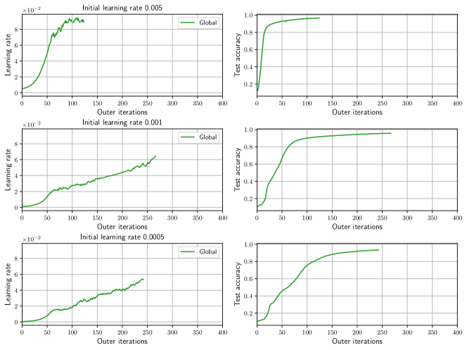
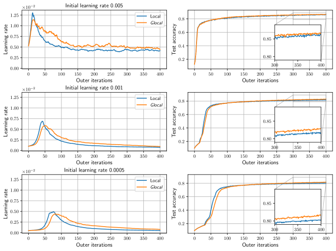
Figure 2 shows learning curves with the transition of learning rates from different initial learning rates on the FMNIST dataset. We can observe that learnable methods automatically find “warmup-and-decay” learning rate schedules, common heuristics in deep learning Loshchilov & Hutter (2017). The glocal approach changes the learning rate more gradually than the local one and shows better final results. The results on other datasets and the transition of other hyperparameters are presented in Appendix C.
- WideResNet on CIFAR-10/100
-
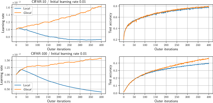
Next, we train WideResNet 28-2 Zagoruyko & Komodakis (2016) using SGD with learnable learning rate and weight-decay rate hyperparameters. The used model has 1.5M parameters and is trained for 20k iterations. As seen in Figure 3, the glocal approach keeps increasing the learning rate to improve the final performance, while the local one fails partially because it cannot look ahead like the glocal method.
4.2 Data Reweighting
Data reweighting task trains a meta module to reweight a loss value to each example to alleviate the effect of class imbalanceLi et al. (2021); Shu et al. (2019). is an MLP, and the inner loss function of the task is , where is cross-entropy loss. is trained on balanced validation data.
We train WideResNet 16-2 on imbalanced CIFAR-10 and CIFAR-100 Cui et al. (2019), which simulate class imbalance. Specifically, the imbalanced data with an imbalance factor of reduces the number of data in the -th class to , where is the number of categories, e.g., 10 for CIFAR-10. As the meta module, we adopt a two-layer MLP with a hidden size of 128, consisting of 385 parameters. Table 3 demonstrates that the glocal approach surpasses the local baseline, indicating its effectiveness.
| Dataset / Imbalance Factor | Local | Glocal |
|---|---|---|
| CIFAR-10 / 50 | 0.605 | 0.710 |
| CIFAR-10 / 100 | 0.565 | 0.665 |
| CIFAR-100 / 50 | 0.280 | 0.315 |
4.3 Analysis
Below, we analyze the factors of the glocal hypergradient estimation using the task in Section 4.1 on the FMNIST dataset.

| w/o HPO | Local | Global | Glocal |
|---|---|---|---|
| 11.4 | 25.1 | 4681.1 | 66.7 |
- Eigenvalues of DMD
-
In Section 3, the existence of eigenpairs whose eigenvalues equal to one was assumed for efficient approximation of a global hypergradient. To see whether it holds in practice, the left panel of Figure 4 shows the eigenvalues obtained by the Hankel DMD at . We can observe two eigenvalues nearly close to (highlighted in orange). Additionally, the right panel of Figure 4 illustrates that modes with other eigenvalues decay rapidly. Because the magnitudes of the modes associated with the eigenvalue of 1 is an order of , other modes can be ignored, numerically supporting the validity of our assumption.
- DMD Configurations
-
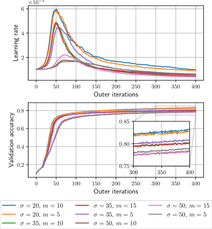
Figure 5 compares the proposed method with different configurations to see how the configurations of the Hankel DMD algorithm, specifically, the number of hypergradients () and the number of stacks per column (), affect the estimation. We can see a clear trend that the number of hypergradients negatively impacts the final performance, contrary to Theorem 3.1, stating that increasing local hypergradients yields better glocal hypergradient estimation. We hypothesize that this gap stems from noise: hypergradients after the hyperparameter change are unstable, and the estimation would be dominated by noise, resulting in degenerated hypergradient estimation and performance in practice. Note that we used this best configuration () found on validation data throughout the experiments in Sections 4.1 and 4.2.
- Runtime
-
Table 4 compares runtime on a machine equipped with an Intel Xeon Gold 5222 CPU and an NVIDIA A100 PCIE 40GB with CUDA 12.3, excluding the time for the just-in-time compiling. Note that because of the limitation of JAX that eigen decomposition for asymmetric matrices on GPU is not yet supported, the computation of the adopted DMD algorithm is suboptimal. Nevertheless, the proposed method achieves significant speedup compared with the global baseline and is only 2.5 times slower than the local one, revealing its empirical efficiency.
5 Discussion and Conclusion
This paper introduced glocal hypergradient estimation, which leverages the virtues of global and local hypergradients simultaneously. To this end, we adopted the Koopman operator theory to approximate a global hypergradient from a trajectory of local hypergradients. The numerical experiments demonstrate the validity of bi-level optimization using glocal hypergradients.
In this work, we have implicitly assumed that the meta criterion converges after enough iterations, and so do hypergradients. This assumption may be strong when a certain minibatch drastically changes the value of the meta criterion, such as adversarial learning. Luckily, we did not suffer from such a problem, probably because we focused our experiments only on supervised learning with sufficiently sized datasets and used full-batch validation data. Introducing stochasticity by the Perron-Frobenius operator Korda & Mezić (2018); Hashimoto et al. (2020), an adjoint of the Koopman operator, would alleviate this limitation, which we leave for future research.
Broader Impact
Bi-level optimization is vital in the applications of machine learning. Compared with traditional black-box counterparts, gradient-based hyperparameter optimization methods are faster and more scalable. As a result, they bring us more efficient machine learning research and development, contributing to reducing energy consumption and democratization in deep learning. We believe that our proposed method will help push it forward, driving the field more sustainable.
Ackenowledgement
This work was supported by JST CREST Grant Number JPMJCR1913 and ACT-X Grant Number JPMJAX210H.
References
- Arbabi & Mezic (2017) Arbabi, H. and Mezic, I. Ergodic theory, dynamic mode decomposition, and computation of spectral properties of the koopman operator. SIAM Journal on Applied Dynamical Systems, 16(4):2096–2126, 2017.
- Baydin et al. (2018) Baydin, A. G., Pearlmutter, B. A., Radul, A. A., and Siskind, J. M. Automatic differentiation in machine learning: a survey. 18(153):1–43, 2018.
- Bengio (2000) Bengio, Y. Gradient-based optimization of hyperparameters. 12(8):1889–1900, 2000.
- Bergstra et al. (2011) Bergstra, J., Bardenet, R., Bengio, Y., and Kégl, B. Algorithms for hyper-parameter optimization. NeurIPS, 2011.
- Bergstra et al. (2013) Bergstra, J., Yamins, D., and Cox, D. Making a science of model search: Hyperparameter optimization in hundreds of dimensions for vision architectures. In ICML, 2013.
- Blondel et al. (2021) Blondel, M., Berthet, Q., Cuturi, M., Frostig, R., Hoyer, S., Llinares-López, F., Pedregosa, F., and Vert, J.-P. Efficient and modular implicit differentiation. 2021.
- Bradbury et al. (2018) Bradbury, J., Frostig, R., Hawkins, P., Johnson, M. J., Leary, C., Maclaurin, D., Necula, G., Paszke, A., VanderPlas, J., Wanderman-Milne, S., and Zhang, Q. JAX: composable transformations of Python+NumPy programs, 2018. URL http://github.com/google/jax.
- Brunton et al. (2022) Brunton, S. L., Budišić, M., Kaiser, E., and Kutz, J. N. Modern koopman theory for dynamical systems. SIAM Review, 64(2):229–340, 2022.
- Choe et al. (2023) Choe, S. K., Mehta, S. V., Ahn, H., Neiswanger, W., Xie, P., Strubell, E., and Xing, E. Making scalable meta learning practical. In NeurIPS, 2023.
- Clanuwat et al. (2018) Clanuwat, T., Bober-Irizar, M., Kitamoto, A., Lamb, A., Yamamoto, K., and Ha, D. Deep learning for classical japanese literature. arXiv, 2018.
- Cui et al. (2019) Cui, Y., Jia, M., Lin, T.-Y., Song, Y., and Belongie, S. Class-balanced loss based on effective number of samples. In CVPR, 2019.
- DeepMind et al. (2020) DeepMind, Babuschkin, I., Baumli, K., Bell, A., Bhupatiraju, S., Bruce, J., Buchlovsky, P., Budden, D., Cai, T., Clark, A., Danihelka, I., Dedieu, A., Fantacci, C., Godwin, J., Jones, C., Hemsley, R., Hennigan, T., Hessel, M., Hou, S., Kapturowski, S., Keck, T., Kemaev, I., King, M., Kunesch, M., Martens, L., Merzic, H., Mikulik, V., Norman, T., Papamakarios, G., Quan, J., Ring, R., Ruiz, F., Sanchez, A., Sartran, L., Schneider, R., Sezener, E., Spencer, S., Srinivasan, S., Stanojević, M., Stokowiec, W., Wang, L., Zhou, G., and Viola, F. The DeepMind JAX Ecosystem, 2020. URL http://github.com/deepmind.
- Dogra & Redman (2020) Dogra, A. S. and Redman, W. Optimizing neural networks via koopman operator theory. In NeurIPS, volume 33, pp. 2087–2097, 2020.
- Domke (2012) Domke, J. Generic methods for optimization-based modeling. 22:318–326, 2012.
- Finn et al. (2017) Finn, C., Abbeel, P., and Levine, S. Model-Agnostic Meta-Learning for Fast Adaptation of Deep Networks. In ICML, 2017.
- Franceschi et al. (2017) Franceschi, L., Donini, M., Frasconi, P., and Pontil, M. Forward and reverse gradient-based hyperparameter optimization. In ICML, 2017.
- Grefenstette et al. (2019) Grefenstette, E., Amos, B., Yarats, D., Htut, P. M., Molchanov, A., Meier, F., Kiela, D., Cho, K., and Chintala, S. Generalized inner loop meta-learning. 2019.
- Hashimoto et al. (2020) Hashimoto, Y., Ishikawa, I., Ikeda, M., Matsuo, Y., and Kawahara, Y. Krylov subspace method for nonlinear dynamical systems with random noise. The Journal of Machine Learning Research, 21(1):6954–6982, 2020.
- Hataya & Yamada (2023) Hataya, R. and Yamada, M. Nyström method for accurate and scalable implicit differentiation. In AISTATS, pp. 4643–4654. PMLR, 2023.
- Hataya et al. (2022) Hataya, R., Zdenek, J., Yoshizoe, K., and Nakayama, H. Meta Approach for Data Augmentation Optimization. In WACV, 2022.
- Hospedales et al. (2021) Hospedales, T., Antoniou, A., Micaelli, P., and Storkey, A. Meta-learning in neural networks: A survey. 44(9):5149–5169, 2021.
- Hutter et al. (2019) Hutter, F., Kotthoff, L., and Vanschoren, J. (eds.). Automatic Machine Learning: Methods, Systems, Challenges. Springer, 2019.
- Kidger & Garcia (2021) Kidger, P. and Garcia, C. Equinox: neural networks in JAX via callable PyTrees and filtered transformations. Differentiable Programming workshop at Neural Information Processing Systems 2021, 2021.
- Kingma & Ba (2015) Kingma, D. P. and Ba, J. L. Adam: a Method for Stochastic Optimization. In ICLR, 2015.
- Koopman (1931) Koopman, B. O. Hamiltonian systems and transformation in hilbert space. Proceedings of the National Academy of Sciences, 17(5):315–318, 1931.
- Korda & Mezić (2018) Korda, M. and Mezić, I. On convergence of extended dynamic mode decomposition to the koopman operator. Journal of Nonlinear Science, 28:687–710, 2018.
- Kutz et al. (2016) Kutz, J. N., Brunton, S. L., Brunton, B. W., and Proctor, J. L. Dynamic Mode Decomposition. Society for Industrial and Applied Mathematics, 2016.
- Larsen et al. (1996) Larsen, J., Hansen, L. K., Svarer, C., and Ohlsson, M. Design and regularization of neural networks: the optimal use of a validation set. In Neural Networks for Signal Processing VI. Proceedings of the 1996 IEEE Signal Processing Society Workshop, 1996.
- Le Cun et al. (1998) Le Cun, Y., Bottou, L., Bengio, Y., and Haffner, P. Gradient-based learning applied to document recognition. 86(11):2278–2324, 1998.
- LeCun et al. (2012) LeCun, Y., Bottou, L., Orr, G., and Müller, K.-R. Efficient BackProp, pp. 9–48. Springer Berlin Heidelberg, 2012.
- Li et al. (2021) Li, M., Zhang, X., Thrampoulidis, C., Chen, J., and Oymak, S. AutoBalance: Optimized Loss Functions for Imbalanced Data. In NeurIPS, 2021.
- Liu et al. (2019) Liu, H., Simonyan, K., and Yang, Y. DARTS: Differentiable architecture search. In ICLR, 2019.
- Lorraine et al. (2020) Lorraine, J., Vicol, P., and Duvenaud, D. Optimizing millions of hyperparameters by implicit differentiation. In AISTATS, 2020.
- Loshchilov & Hutter (2017) Loshchilov, I. and Hutter, F. SGDR: Stochastic gradient descent with warm restarts. In ICLR, 2017. URL https://openreview.net/forum?id=Skq89Scxx.
- Lu & Tartakovsky (2020) Lu, H. and Tartakovsky, D. M. Prediction accuracy of dynamic mode decomposition. SIAM Journal on Scientific Computing, 42(3):A1639–A1662, 2020.
- Luketina et al. (2016) Luketina, J., Berglund, M., Greff, K., and Raiko, T. Scalable gradient-based tuning of continuous regularization hyperparameters. In ICML, 2016.
- Maclaurin et al. (2015) Maclaurin, D., Duvenaud, D., and Adams, R. P. Gradient-based Hyperparameter Optimization through Reversible Learning. In ICML, 2015.
- Manojlović et al. (2020) Manojlović, I., Fonoberova, M., Mohr, R., Andrejčuk, A., Drmač, Z., Kevrekidis, Y., and Mezić, I. Applications of koopman mode analysis to neural networks. arXiv, 2020.
- Mezić (2005) Mezić, I. Spectral properties of dynamical systems, model reduction and decompositions. Nonlinear Dynamics, 41:309–325, 2005.
- Micaelli & Storkey (2021) Micaelli, P. and Storkey, A. Gradient-based hyperparameter optimization over long horizons. In NeurIPS, 2021.
- Pedregosa (2016) Pedregosa, F. Hyperparameter optimization with approximate gradient. In ICML, 2016.
- Rajeswaran et al. (2019) Rajeswaran, A., Finn, C., Kakade, S., and Levine, S. Meta-Learning with Implicit Gradients. In NeurIPS, 2019.
- Redman et al. (2022) Redman, W. T., Fonoberova, M., Mohr, R., Kevrekidis, Y., and Mezić, I. An operator theoretic view on pruning deep neural networks. In ICLR, 2022.
- Sakamoto et al. (2023) Sakamoto, K., Ishibashi, H., Sato, R., Shirakawa, S., Akimoto, Y., and Hino, H. Atnas: Automatic termination for neural architecture search. Neural Networks, 166:446–458, 2023.
- Shu et al. (2019) Shu, J., Xie, Q., Yi, L., Zhao, Q., Zhou, S., Xu, Z., and Meng, D. Meta-weight-net: Learning an explicit mapping for sample weighting. In NeurIPS, 2019.
- Smith et al. (2018) Smith, S. L., Kindermans, P.-J., and Le, Q. V. Don’t decay the learning rate, increase the batch size. In ICLR, 2018. URL https://openreview.net/forum?id=B1Yy1BxCZ.
- Wu & He (2018) Wu, Y. and He, K. Group normalization. In ECCV, 2018.
- Wu et al. (2018) Wu, Y., Ren, M., Liao, R., and Grosse., R. Understanding short-horizon bias in stochastic meta-optimization. In ICLR, 2018.
- Xiao et al. (2017) Xiao, H., Rasul, K., and Vollgraf, R. Fashion-mnist: a novel image dataset for benchmarking machine learning algorithms. arXiv, 2017.
- Zagoruyko & Komodakis (2016) Zagoruyko, S. and Komodakis, N. Wide Residual Networks. In BMVC, 2016.
- Zhang et al. (2021) Zhang, M., Su, S. W., Pan, S., Chang, X., Abbasnejad, E. M., and Haffari, R. idarts: Differentiable architecture search with stochastic implicit gradients. In ICML, 2021.
Appendix A Additional Discussion on Theorem 3.1
The first half of the proof of Theorem 3.1 depends on the theorem 3.6 of Lu & Tartakovsky (2020), which shows Equation 22 without equality holds if ’s spectral radius . This condition can be relaxed to , and then Equation 22 holds. in Theorem 3.1 can be given as
| (25) |
where and depends on the number of hypergradients.
Appendix B Detailed Experimental Settings
Throughout the experiments, the batch size of training data was set to 128.
B.1 Optimizing Optimizer Hyperparameters
- LeNet
-
We set the number of filters in each convolutional layer to 16 and the dimension of the following linear layers to 32. The leaky ReLU is used as its activation.
- WideResNet
- Validation data
-
We separated 10% of the original training data as validation data.
B.2 Data reweighting
- WideResNet
-
We modified the original WideResNet 16-2 in Zagoruyko & Komodakis (2016) as follows: replacing the batch normalization with group normalization and adopting the leaky ReLU as the activation function. The model was trained with an inner optimizer of SGD with a learning rate of 0.01, momentum of 0.9, and weight decay rate of 0.
- Valiation data
-
We separated 1000 data points from the original training dataset to construct a validation set.
Appendix C Additional Experimental Results
Figures 6 and 7 present the transition of the learning rate hyperparameter and test accuracy curves of LeNet on MNIST and KMNIST. Except for the case of MNIST with the initial learning rate of , the curves are similar among MNIST variants.
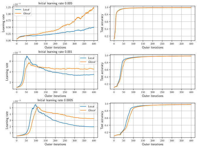
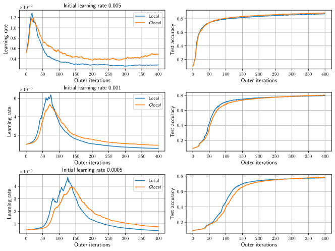
Figure 8 shows the development of momentum and weight decay hyperparameters of LeNet on FMNIST, whose learning rate hyperparameter development is presented in Figure 2. The initial values of these hyperparameters were set to and . Although the learning rates optimized by local and glocal hypergradients are alike, momentum and weight decay change differently: glocal hypergradients yield milder changes. We can observe that as the initial learning rate decreases, the peak of momentum increases, which can be explained by that the effective learning rate is inversely proportional to one minus momentum Smith et al. (2018).
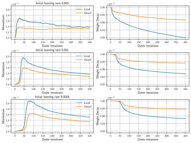
Figure 9 displays the failures of the global approach. As it needs to keep using a high learning rate for a long horizon, the training fails because the model parameters explode.