Comprehensive study of magnetic field evolution in relativistic jets based on 2D simulations

Abstract

We use two-dimensional particle-in-cell simulations to investigate the generation and evolution of the magnetic field associated with the propagation of a jet for various initial conditions. We demonstrate that, in general, the magnetic field is initially grown by the Weibel and Mushroom instabilities. However, the field is saturated by the Alfvén current limit. For initially non-magnetized plasma, we show that the growth of the magnetic field is delayed when the matter density of the jet environment is lower, which are in agreement with simple analytical predictions. We show that the higher Lorentz factor ($\gtrsim 2$) prevents rapid growth of the magnetic fields. When the initial field is troidal, the position of the magnetic filaments moves away from the jet as the field strength increases. The axial initial field helps the jet maintain its shape more effectively than the troidal initial field.

I Introduction:

Relativistic jets are often found in astrophysical objects such as pulsars, gamma ray bursts (GRB), and active galactic nuclei (AGN). They are magnetized because synchrotron radiation has been detectedGabuzda (2019a). When a relativistic jet interacts with its environment, several instabilities grow. These may be responsible for the growth of the magnetic field. For example, the Weibel instability has been shown to develop in non-magnetized jets Weibel (1959). This instability occurs when the particle velocity distribution function (PDF) is anisotropic. The Weibel instability helps to make the PDF isotropic by generating magnetic fields and currents in the plasma to deflect the plasma particles Fujita, Kato, and Okabe (2006). The shear of the jet boundary also causes instabilities such as the kinetic Kelvin-Helmholtz instability (kKHi) and the mushroom instability (MI); the MI develops perpendicular to the direction of the jet Rieger and Duffy (2021); Meli and i. Nishikawa (2021); Alves, Zrake, and Fiuza (2018). We note that the MI instability is a Rayleigh-Taylor instability (RTi) caused by electrons/ions on the kinetic scale. After the initial development, the magnetic field gradually saturates, which has been studied for simple settings Kato (2005); Fujita, Kato, and Okabe (2006).

The method of simulating plasma phenomena using moving particles was developed by a group of scientists, including Buneman, Hockney, Birdsall, and Dawson. In this method or particle-in-cell (PIC) simulations, the particles are controlled by the electromagnetic field produced by their own movement and by any external fields. The electromagnetic field alters the particle’s trajectory in a self-consistent manner. The method does not analyze bulk/fluid dynamics like the magnetohydrodynamics (MHD) code, but instead takes a kinematic approach to the problem and complements the fluid approach. However, it can be challenging for the PIC simulations to handle a wide range of scales, spanning from microphysics to macro/global dynamics, although it is necessary to study AGN jets Nishikawa et al. (2021).

In this letter, we present the results of two-dimensional (2D) PIC simulations that reveal magnetic field generation and its impact on jet evolution. We study the evolution of the field in the cross-section of the jet, which is an analysis unfeasible through traditional fluid-based approaches. We focus on a numerical study of basic plasma phenomena rather than possible applications to AGN jets, since current computing power does not allow us to reproduce a realistic AGN jet on the scale of $>$ pc using PIC simulations.We run simulations with different setups of magnetized and unmagnetized jets. Our simulations are similar to those of Kawashima et al. Kawashima et al. (2022), where they focused mainly on the effect of magnetic reconnection on the heating of the jet. They showed that the x-point of the magnetic reconnection moves inward over time, which helps to maintain the spine of the jet. On the contrary, we study the effects of different magnetic field structures on the jet propagation and the instability developed along the jet. Since our main goal is to reveal the parameter dependence of plasma instabilities, we need to cover a wide range of parameters. Therefore, we perform 2D PIC simulations instead of 3D. We also note that we can discuss the $z$ components of the magnetic field and velocity even though our 2D simulations deal with the $xy$ cross section of the jet.

II simulation setup:

Our code has two spatial and three velocity dimensions (2D3V). The simulation plane is taken on the $xy$ plane perpendicular to the $z$-axis. The jet propagates in the $z$-direction. We adopt a simulation setup similar to that of Kawashima et al.Kawashima et al. (2022), and the parameters are shown in Table 1. The ion mass $m_{i}$ to electron mass $m_{e}$ ratio is $m_{i}/m_{e}=16$ in most runs and the thermal velocity of the plasma particles in the $x$, $y$ and $z$ directions is $v_{\rm thr}=0.1\>c$, where $c$ is the light velocity. We used this ion-electron mass ratio of $m_{i}/m_{e}=16$ because a realistic mass ratio requires more time and space resolution, and it is difficult to cover a wide range of initial parameters. However, we perform simulations of $m_{i}/m_{e}=1836$ for a few representative cases to check consistency (section E.3).Different initial bulk jet velocities $0.25\>c\leq V_{c0}\leq 0.948\>c$ are applied in the $z$-direction. The corresponding Lorentz factor is given by $\gamma_{0}=1/\sqrt{1-V_{c0}^{2}/c^{2}}$. Since we also studied the effects of different jet environments as in Alves et al.Alves et al. (2014), we assume different ratios of the initial density of the jet ($n_{\rm jet}$) to that of the surrounding environment ($n_{\rm out}$). We set the number density of the jet plasma to $n_{\rm jet}=100$. We consider zero, troidal, and axial fields for the initial magnetic field, and the characteristic value is given by $b_{0}$. Even when $b_{0}=0$, magnetic fields are generated around the jet boundary. When the initial magnetic field is toroidal, the $x$ and $y$ components are given by $b_{x0}=(y-y_{jc})b_{0}/[1+(r/a)^{2}]$, and $b_{y0}=(x-x_{jc})b_{0}/[1+(r/a)^{2}]$, respectively, where $(x_{jc},y_{jc})$ is the jet axis and $a$ is the jet radius. For models with a zero or axial initial magnetic field, the field strength is spatially uniform and is given by $b_{0}$.

The grid sizes are $\Delta x=\Delta y=1$, plasma frequency is $\omega_{pe}=0.05$, Debye length is $\lambda_{D}=0.05$ , skin depth is $\lambda_{s}=c/\omega_{\rm pe}=20$, simulation time-step is $dt=0.5$, simulation box size is $800\times 800$, and total simulation time is $t=500$. The time unit is $\omega_{pe}^{-1}$. The jet axis is at $(x_{jc},y_{jc})=(400,400)$ except for Run 11 and the initial jet radius is $a=100$. We use 100 electron-ion pairs in each cell. Periodic boundary conditions are adopted in the $x$ and $y$-directions for both particles and electromagnetic fields. To verify convergence, similar runs were performed with more particles in each cell (150 and 200 particles), and we confirmed that the results converged as the number of particles in each cell increased.

We note that the width of real astrophysical jets is $\gtrsim 10^{16}\rm\>cm$,Hada et al. (2011) while the phyical diameter of the jet used in our simulation is about $10\>c/\omega_{pe}\sim 10^{5}\rm\>cm$, (if we assume the number density of the jet to be about $10^{4}\rm\>cm^{-3}$)Kawashima et al. (2022). Thus, our length scale is much smaller compared to the real jet.

Table 1: Simulation Parameters

Run	Initial magnetic field	$V_{c0}$	$\gamma_{0}$	$n_{\rm out}$	$n_{\rm jet}/n_{\rm out}$
1	$b_{0}=0.0$	$0.9c$	2.3	100	1
5	Toroidal, $b_{0}=0.01$	$0.9c$	2.3	100	1
6	Toroidal, $b_{0}=0.05$	$0.9c$	2.3	100	1
8	Toroidal, $b_{0}=0.01$	$0.5\rm c$	1.16	100	1
9	Toroidal, $b_{0}=0.01$	$0.25\rm c$	1.033	100	1
10	Toroidal, $b_{0}=0.025$	$0.5\rm c$	1.16	100	1
11	Toroidal, $b_{0}=0.01$	$0.5\rm c$	1.16	100	1
12	Axial, $b_{0}=0.01$	$0.5\rm c$	1.16	100	1
13	Axial, $b_{0}=0.025$	$0.5\rm c$	1.16	100	1
17	Axial, $b_{0}=0.01$	$0.9\rm c$	2.3	100	1
30	$b_{0}=0.0$	$0.5\rm c$	1.16	100	1
31	$b_{0}=0.0$	$0.5\rm c$	1.16	80	1.25
32	$b_{0}=0.0$	$0.5\rm c$	1.16	60	1.66
33	$b_{0}=0.0$	$0.5\rm c$	1.16	40	2.5
34	$b_{0}=0.0$	$0.5\rm c$	1.16	20	5.0
36	$b_{0}=0.0$	$0.866\rm c$	2	100	1
37	$b_{0}=0.0$	$0.948\rm c$	10	100	1

III simulation results and discussion:

III.1 Jet evolution

We show overall jet evolution by taking Run 8 as the fiducial model (Figure 1). Initially, particles in the simulation box have a bulk velocity in the $+z$ direction. Therefore, electrons carry current in the $-z$ direction and ions carry current in the opposite direction. As a result of the anisotropy of the PDF, filaments are formed in the $z$-direction by the Weibel instability; the main filaments are formed in the jet radius and other filaments are formed in the surrounding region (Figure 1(a)). The rings shown in Figures 1(a)-(c) are the cross-section of the filaments. Magnetic fields are generated around the currents associated with the filaments. The filaments attract each other and merge together by magnetic force (Figures 1(b) and (c)), which increases the current. Due to the amplification of the magnetic field, the particles become more deflected. Both the current and the magnetic field continue to grow exponentially through the mergers of filaments until saturation is reached. The current tubes merge until $t\sim 200$. Then they stop growing. The magnetic field also saturates around that time (Figure 1(e)).

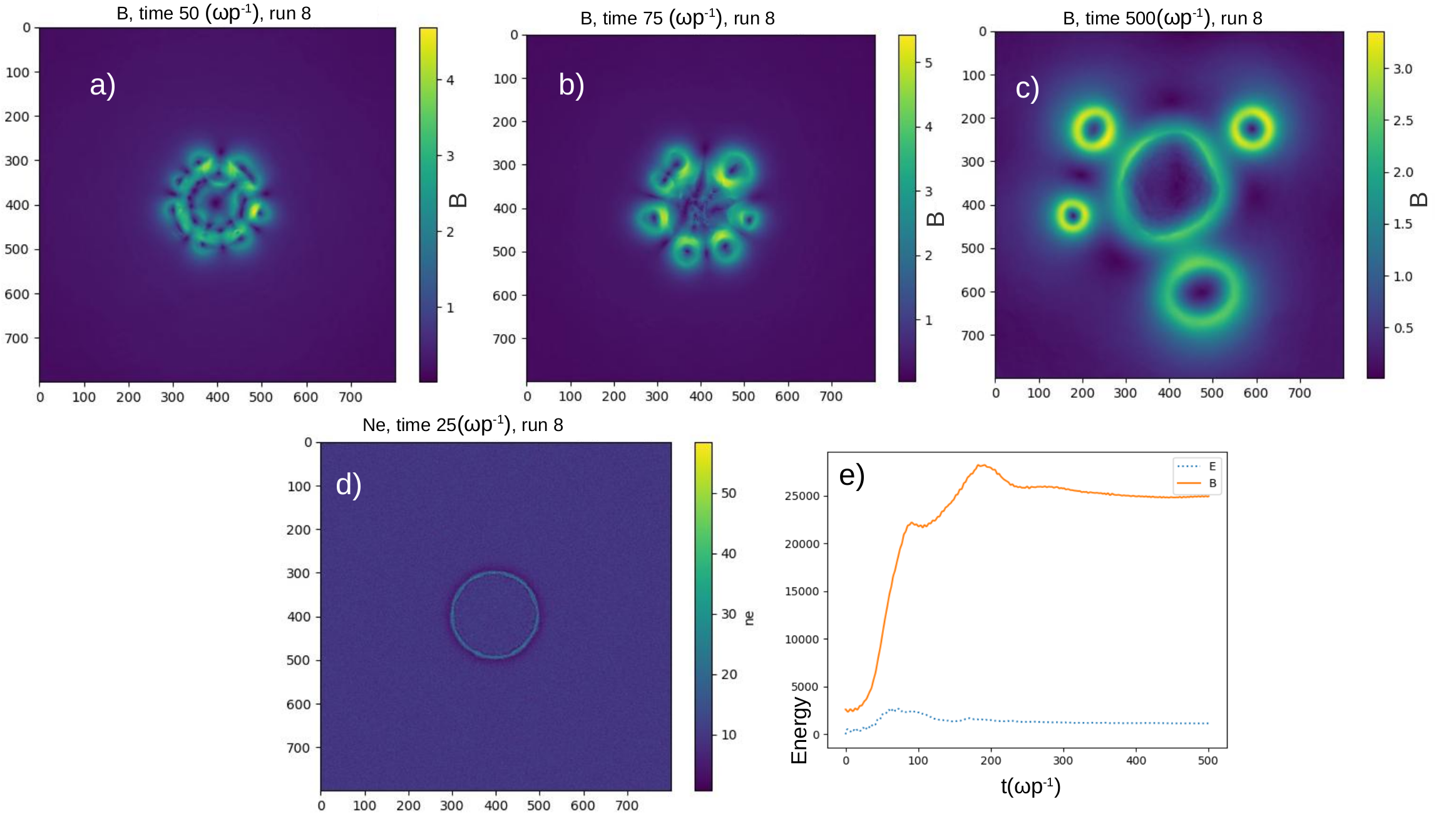
Figure 1: Magnetic field evolution for Run 8 ($\gamma_{0}=1.16$ and $b_{0}=0.01$). The initial jet velocity is $0.5\>c$ normal to the paper. (a) Magnetic field strength at $t=50$, (b) $t=75$, and (c) $t=500$. In panel (a) the field is generated and in panels (b), (c) and (d) the merging of filaments at the jet boundary is seen. (d) Electron number density at the time $t=25$. Electrons are slightly clustered around the jet. (e) Evolution of total magnetic energy (orange solid line) and electric energy (cyan dotted line).

Figure 1(d) shows the electron density distribution at time $t=25$, which is almost uniform but slightly clustered around the jet. After the saturation ($t\sim 200$), the size of the current tubes remains almost the same. There is a small saturation before $t\sim 100$ (Figure 1(e)), which is due to the saturation of the magnetic field structures inside the jet.

III.2 Saturation mechanism

The saturation we showed above may be explained by the model of KatoKato (2005). A cylindrical beam is characterized by its radius $r$ and current $I$, where $I=\pi r^{2}J$ and $J$ is the current density. The average magnetic field within the beam can be written as $B=\sqrt{2}\pi rJc=\sqrt{2}\pi I/(rc)$. Due to the coalescence of the filaments with each other, both the current and the magnetic field of the filaments increase exponentially, and the filament radius also increases. However, this growth stops when the current reaches the Alfven current $I_{A}=\left\langle I_{0}\gamma_{0}\beta_{\parallel}\right\rangle$, where $I_{0}=m_{e}c^{3}e$, $-e$ is the electron charge. $\beta_{\parallel}$ is the $z$ component of $\beta$ (velocity normalized by $c$), $\gamma=(1-\beta^{2})^{-1/2}$, and $\left\langle\right\rangle$ denotes averaging over the filament volume. This is because the movement of the particles in the current is impeded by the self-generated magnetic field.

From the Alfven current, the maximum magnetic field is calculated as:

$$B_{\rm max}=\frac{\sqrt{2}}{rc}I_{\rm A}=\frac{\sqrt{2}\left\langle\gamma\beta_{\parallel}\right\rangle}{r/I_{0}}B_{\ast}\>,$$ (1)

where $B_{\ast}$ is the magnetic field strength defined by $B_{\ast}=m_{e}c\omega_{\rm pe}e\cong 3.2\times 10^{-1}\sqrt{n_{e}}[\rm G]$.

We compare the maximum or saturated magnetic field around the jet obtained by the simulations with the theory. Since the model of KatoKato (2005) does not include background magnetic fields, we compare it with the results of Run 31, which has the same initial parameters as Run 8 except for the zero initial magnetic field ($b_{0}=0$); Run 31 shows a similar evolution to Run 8. We find that while the maximum magnetic field in the simulation at time $t=200$ is 2.5, equation (1) gives $B_{\rm max}=2.87$ for $\gamma_{0}=1.16$, $\beta_{\parallel}=0.5$, and $I_{0}=101.58$. Thus, they are close to each other. This is almost the same for Run 8 with non-zero but small $b_{0}$.

III.3 Jet and environment density

For initially non-magnetized plasma, we study the effects of different ambient densities on the jet evolution. First, we discuss analytically the growth rate of the MI. We use a fluid model of Alves et. al.Alves et al. (2015) to obtain the growth rate for different density contrasts. While they only gave results when there was no density contrast, we consider the cases where the densities are different. Here we evaluate the growth rate for the different $n_{\rm jet}/n_{\rm out}$ by considering a linear perturbation theory.

We consider two adjacent fluids of different densities; their values are represented by the indices $+$ and $-$, respectively, and their initial or unperturbed values are represented by the index 0. The velocity of the sheared plasma flow is $\vec{v}_{0}=v_{0}(x)\vec{e}_{z}$, where $\vec{e}_{z}$ is the unit vector in the $z$ direction. Considering charge and current neutrality, the equal density ($n_{0}=n_{i0}=n_{e0}$) and equal velocity ($v_{0}=v_{i0}=v_{e0}$) conditions are applied to ensure the initial equilibrium between ions ($i$) and electrons ($e$). For a fluid quantity $f$ we assign a perturbation $f=f_{0}+\delta f$ with $\delta f(x,y,t)=\delta f(x)e^{-i\omega t+iky}$, where $\omega$ ($\in\mathbb{C}$) is the frequency and $k$ ($\in\mathbb{R}$) is the wave number. All zeroth order quantities are assumed to be zero except $n_{0}(x)$ and $v_{0}(x)$. The perturbed current densities in the $x$, $y$, and $z$ directions are $\delta j_{x}=-e(1+m_{e}/m_{i})n_{0}\delta v_{ex}$, $\delta j_{y}=-e(1+m_{e}/m_{i})n_{0}\delta v_{ey}$, and $\delta j_{z}=-e(1+m_{e}/m_{i})(n_{0}\delta v_{ez}+\delta nv_{0})$, respectively. A step velocity shear and density profile of the form $v_{0}(x)=v^{-}+(v^{+}-v^{-})\mathcal{H}$ and $n_{0}(x)=n^{-}+(n^{+}-n^{-})\mathcal{H}$ are used, where $\mathcal{H}$ is a Heaviside step function. By integrating $\epsilon.\delta\mathrm{E}=0$ for $x\neq 0$, where $\epsilon_{ij}=\sum_{m=0}^{2}C_{ij,m}[\omega,k_{y},v_{0}(x),n_{0}(x))]\partial_{x^{m}}$ ($C_{ij,m}$ is constant factors of equation) and $\delta\mathrm{E}=(\delta E_{y},\delta E_{z}$), and using the continuity of $\delta E_{y}$ and $\delta E_{z}$ at the shear interface, we discover solutions that correspond to evanescent waves known as $\delta E_{y,z}=\delta E_{y,z}(0)e^{-k^{\pm}_{\bot}|x|}$. $k^{\pm}_{\bot}=\sqrt{D^{\pm}_{\bot}/c^{2}}$, $D^{\pm}_{\bot}=c^{2}k^{2}+\omega_{pe\pm}^{2}/\gamma_{0\pm}-\omega^{2}$, $\omega_{pe\pm}^{2}=e^{2}n^{\pm}(1+m_{e}/m_{i})/\epsilon_{0}m_{e}$, and $\gamma_{0\pm}=1/\sqrt{1-(v_{0}^{\pm}/c)^{2}}$. By evaluating the difference of the electric field derivatives across the shear interface, we obtain $\mathrm{I}.\delta\mathrm{E_{0}}=0$, where $\delta\mathrm{E_{0}}=(\delta E_{y}(0),\delta E_{z}(0))$, $I_{ij}=a_{ij}^{+}k_{\bot}^{+}+a_{ij}^{-}k_{\bot}^{-}$, $a^{\pm}_{11}=(\omega^{2}-\omega^{2}_{pe\pm}/\gamma_{0\pm})D^{\pm-1}_{\bot}$, $a^{\pm}_{12}=-(kv_{0}/\omega)(\omega^{2}_{pe\pm}/\gamma_{0\pm})D^{\pm-1}_{\bot}$ , $a^{\pm}_{21}=a^{\pm}_{12}$, and $a^{\pm}_{22}=-1-(k^{2}c^{2}/\omega^{2}-1)(\omega^{2}_{pe\pm}/\gamma_{0\pm})(v_{0}^{2}/c^{2})D^{\pm-1}_{\bot}$. We obtain the growth rate ${\rm Im}(\omega)$ for different $n_{+}/n_{-}$ ($n_{\rm jet}/n_{\rm out}$) by numerically solving

$$\mathrm{det}(\mathrm{I})=0$$ (2)

Figure 2(a) shows the obtained growth rate of the MI or the imaginary part of the frequency ($\omega$) for different density contrasts. The growth rate is smaller for $n_{+}/n_{-}=2$ than for $n_{+}/n_{-}=1$. For comparison, in Figure 2(b) we show our simulation results and the difference in the evolution of the magnetic field energy, when the density ratio $n_{\rm jet}/n_{\rm out}$ varies from 1.25, to 5 (Runs 31-34, Table 1). The saturation time is delayed as the ratio increases, which means that the initial growth rate is smaller for the larger $n_{\rm jet}/n_{\rm out}$. This is qualitatively consistent with Figure 2(a). We note that laser plasma experiments Ma et al. (2020) have also shown that the saturation time is delayed as $n_{\rm PDG}/n_{\rm out}$ (in which PDG stands for Plasma Density Grating. ) increases. Runs 30-34 are performed to study the evolution of the jet for the different surrounding densities (Table 1). Figure 3 are the magnetic field distributions for these runs and show the influence of the surrounding matter on the jet. As $n_{\rm jet}/n_{\rm out}$ increases from Run 30 to 34, the jet radius increases. In our simulations, the thermal velocity of the particles surrounding the jet is constant ($v_{\rm thr}=0.1\>c$). Thus, the decrease of $n_{\rm out}$ or the increase of $n_{\rm jet}/n_{\rm out}$ corresponds to the decrease of the external pressure of the jet. The difference in jet radius between Runs 30–34 indicates the importance of the external pressure for jet confinement. This effect has actually been discussed for astrophysical jets Begelman and Cioffi (1989); Gourgouliatos and Komissarov (2018).

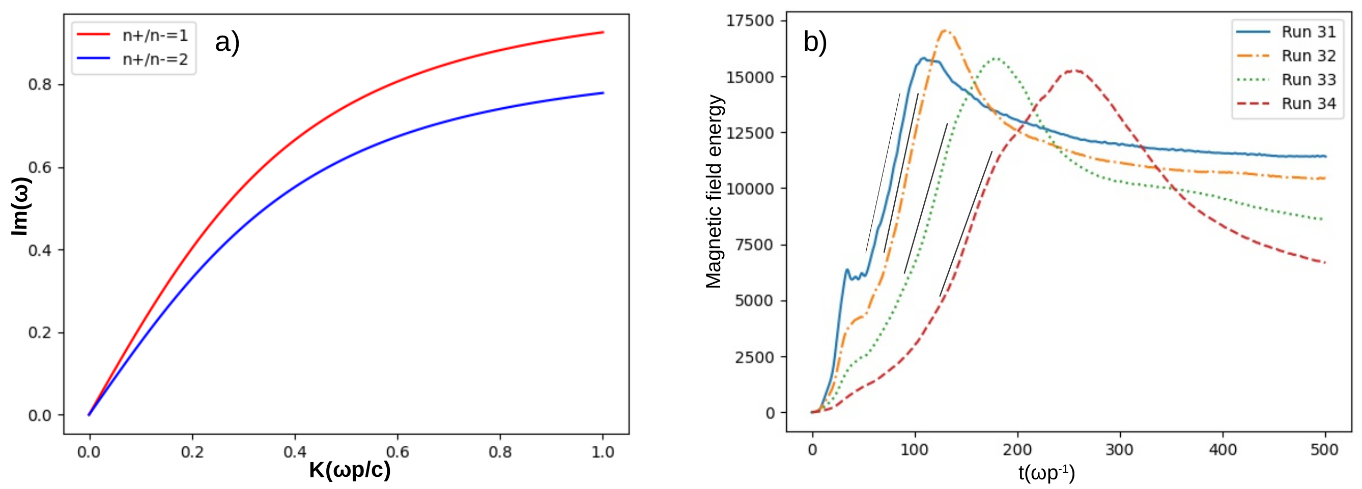
Figure 2: (a) The growth rate of the MI obtained by solving equation (2) for $n_{+}/n_{-}=1$ and 2. (b) Simulated evolution of the total magnetic field energy for different outer jet densities. The ratio $n_{\rm jet}/n_{\rm out}$ increases from Run 31 to Run 34. The results for Run 30 are almost the same as Run 31. The initial magnetic field is assumed to be 0, and the initial jet Lorentz factor is assumed to be $\gamma_{0}=1.16$. The results show that as the outer plasma density decreases, the saturation time delays and the growth rate decreases (see the gray segments representing the MI growth). There is a slight saturation around time $t=32.5$ due to instabilities in the jet and the saturation of the filaments.

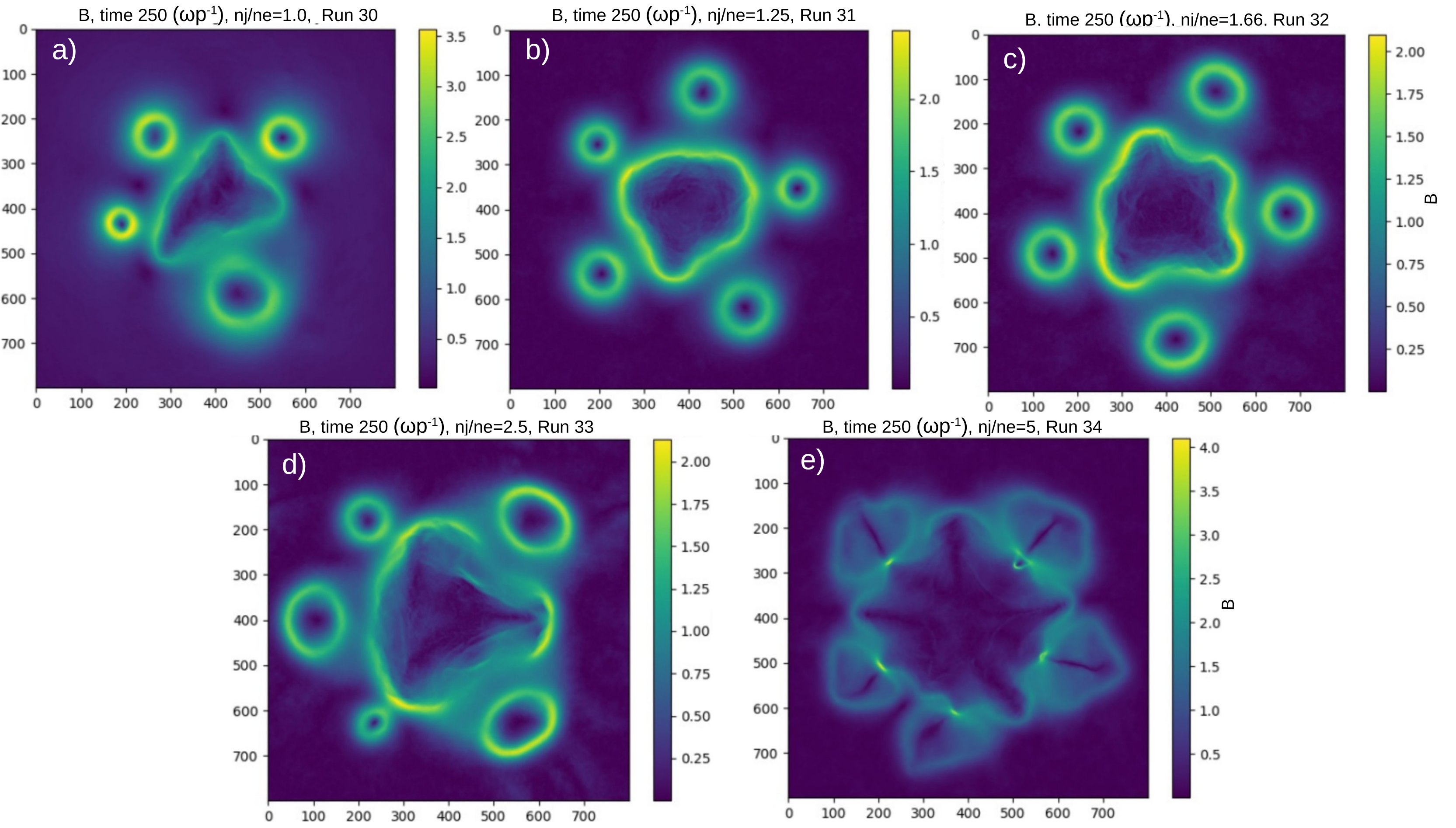
Figure 3: Distribution of the magnetic field strength for different $n_{\rm jet}/n_{\rm out}$ at $t\sim 250$ for (a) Run 30, (b) Run 31, (c) Run 32, (d) Run 33, and (e) Run 34

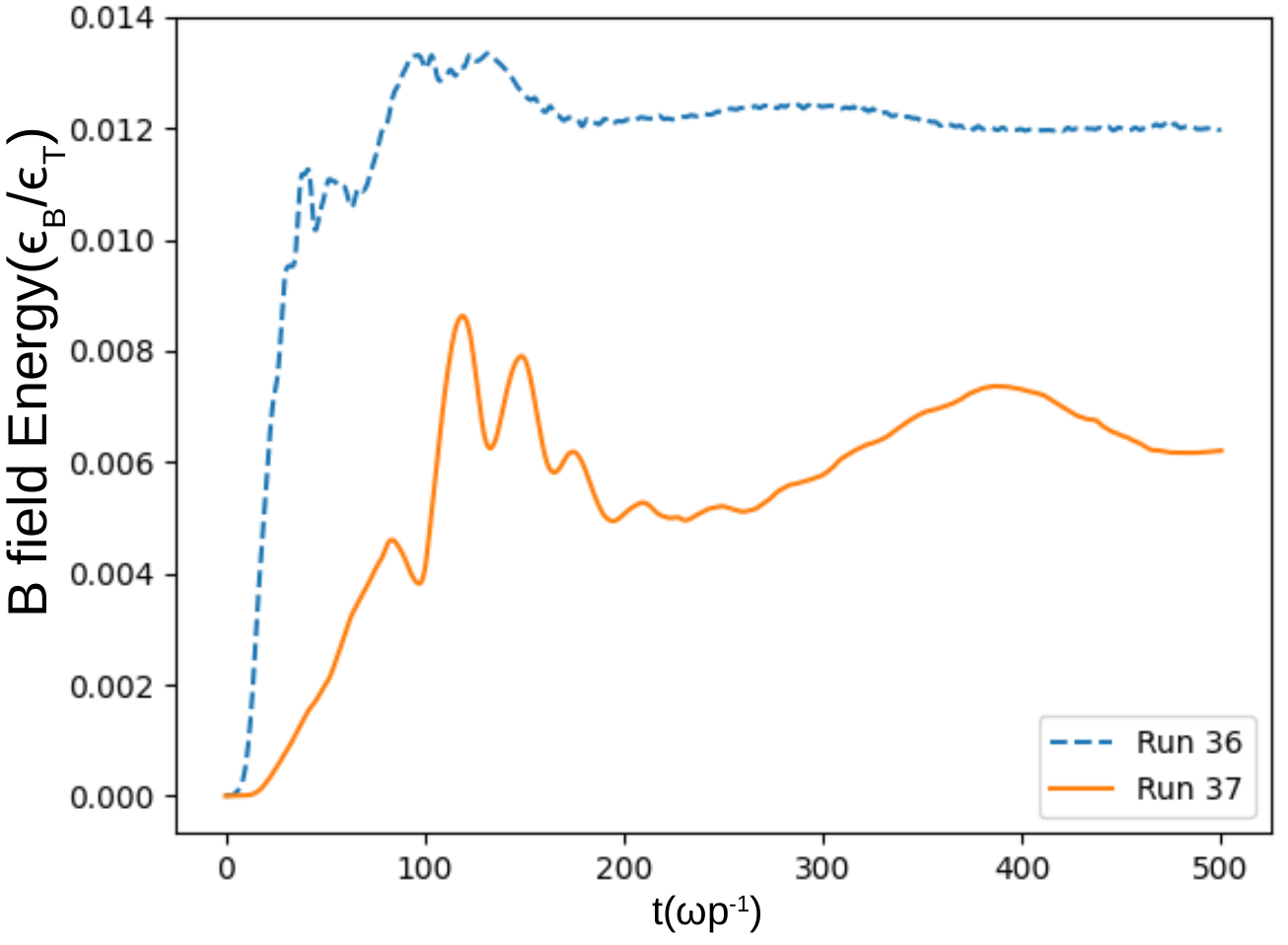
Figure 4: Evolution of magnetic field energy for different Lorentz factors ($\gamma_{0}=2$ for Run 36 and $\gamma_{0}=10$ for Run 37).

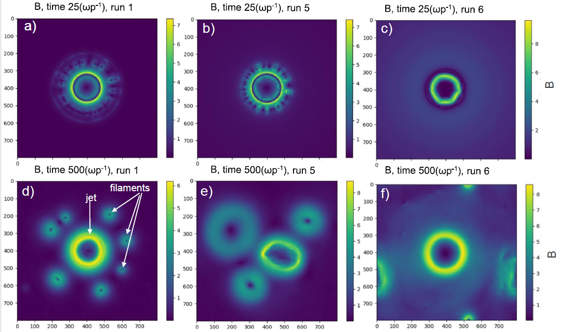
Figure 5: Distribution of the magnetic field strength. The top refers to the results at $t=25$, while the bottom refers to those at $t=500$. From the left row to the right row the results for (a), (d) Run 1, (b), (e) Run 5 and (c), (f) Run 6are shown. The initial values are $b_{0}=0$ for Run 1, $0.01$ for Run 5 and $0.05$ for Run 6. The Lorentz factor is $\gamma_{0}=2.3$ for all runs. In Run 6, panel (f), the filaments are formed far away from the jet. We note that compared to Run 8 ($\gamma_{0}=1.16$ and $b_{0}=0.01$, see Figure 1), the initial jet velocity is larger and consequently the generated magnetic field is also larger. In panel (d) the jet and some filaments are marked.

III.4 The influence of Larger Lorentz factor for non-magnetized plasma

For initially non-magnetized plasma, Alves et al.Alves et al. (2015) analytically studied the effect of the Lorentz factor on the growth rate of the MI for a plane geometry as shown in their Figure 1(b). They showed that the growth rate of the MI behaves as $\gamma_{0}^{-1/2}$ in the range $\gamma_{0}\gtrsim 2$, while it is an increasing function of $\gamma_{0}$ for $\gamma_{0}\lesssim 2$. To investigate whether their results can be applied to our jet geometry, we study the growth rate of the magnetic field energy with different jet Lorentz factors of $\gamma_{0}=2$ and $\gamma_{0}=10$ (Runs 36 and 37). We note that we give the thermal velocity in our simulations ($v_{\rm out}=v_{\rm thr}=0.1c$), and the influence is relatively strong when there is no initial magnetic field. Therefore, we make a comparison only for $\gamma_{0}\geq 2$, since the thermal velocity can be ignored. Figure 4 shows the results. Since the initial magnetic field is set to zero, the magnetic field is generated only by the motion of the jet particles. For comparison, the curve for $\gamma_{0}=2$ (Run 36) is multiplied by 10. As can be seen, the curve for $\gamma_{0}=2$ is steeper than that for $\gamma_{0}=10$ (Run 37) during the initial growth phase ($t\lesssim 30$ for Run 36 and $t\lesssim 100$ for Run 37). This shows that a very large Lorentz factor prevents rapid growth of magnetic fields. In fact, we calculate the growth rates and find that $\Gamma=0.063$ for Run 37 and $\Gamma=0.15$ for Run 36 and the ratio is $0.15/0.063=2.38$ which is consistent with the theory $(\Gamma\propto\gamma_{0}^{-1/2}$ or $\sqrt{10}/\sqrt{2}=2.24)$.

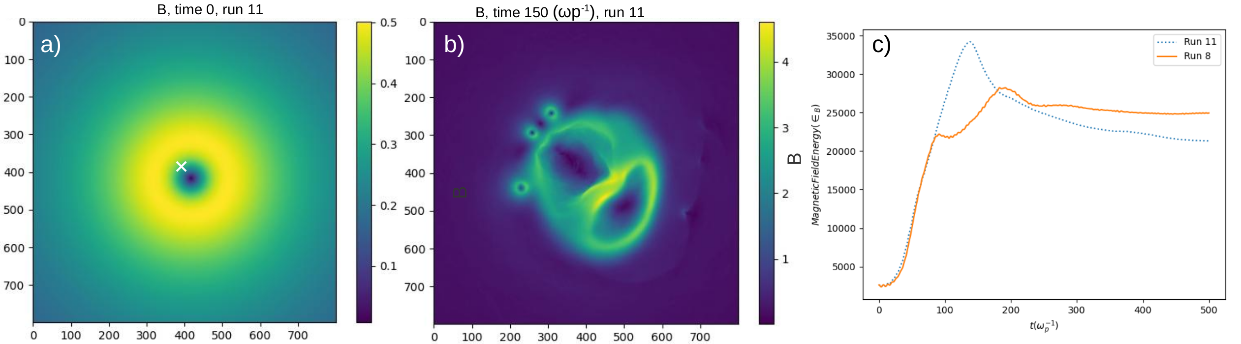
Figure 6: Effect of the off-center initial magnetic field on the instability. (a) Magnetic field distribution for Run 11 at $t=0$. The field is toroidal and surrounds the jet cross section, but is shifted +20 in the $x$, $y$ directions. The cross represents the center of the jet. (b) Magnetic field distribution for Run 11 at $t\sim 150$. No filaments are formed in the lower right corner of the jet, in contrast to the filaments in the upper left corner. (c) Evolution of the total magnetic field energy for Runs 8 (fiducial model) and 11.

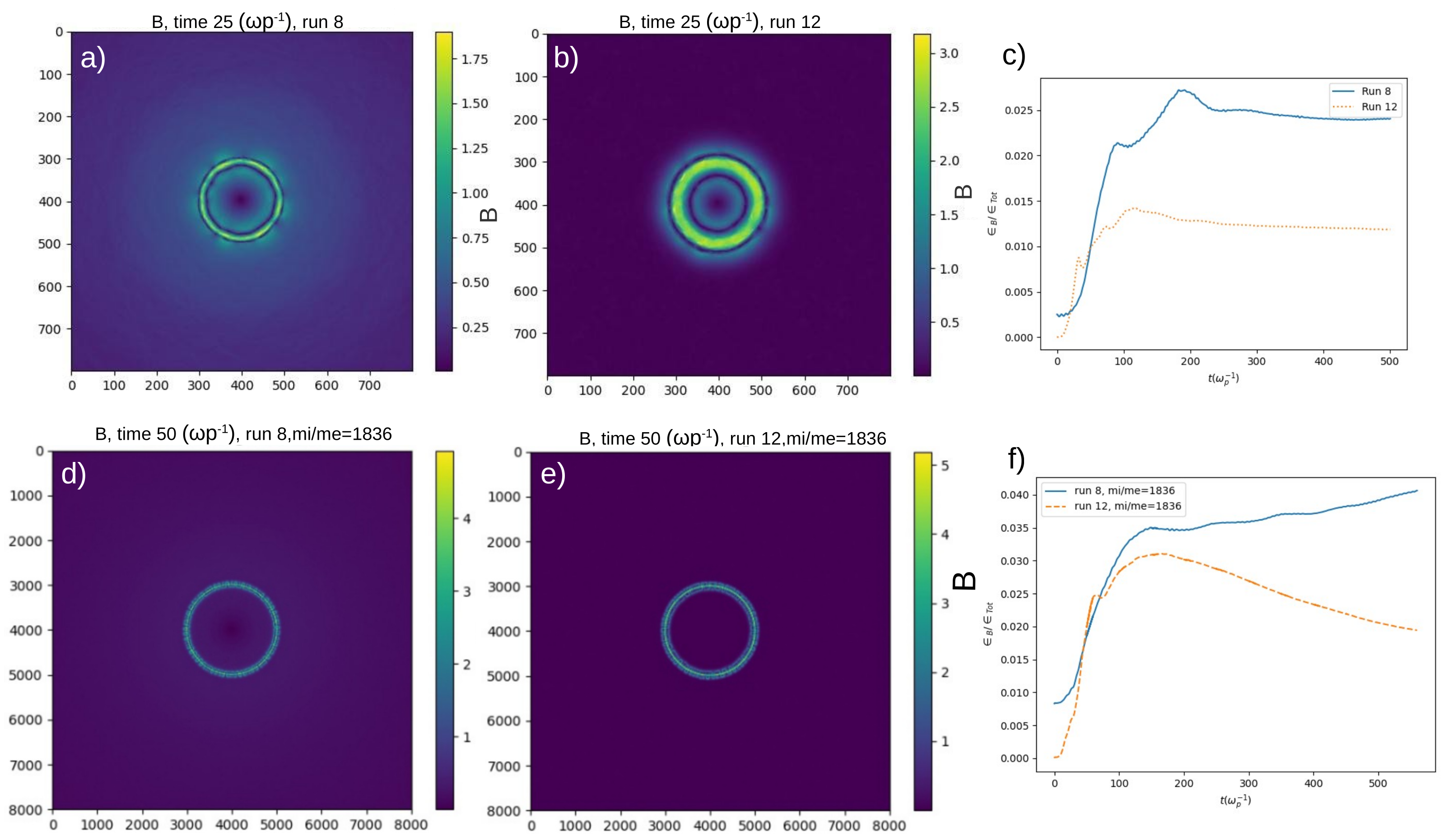
Figure 7: Effect of the initial magnetic field topology on the instability. Magnetic field distribution at time $t=25$ for the case of (a) toroidal initial magnetic field (Run 8; $\gamma_{0}=1.16$ and $b_{0}=0.01$) and (b) axial initial magnetic field (Run 12; $\gamma_{0}=1.16$ and $b_{0}=0.01$). The axial initial magnetic field generates more magnetic field at later times and also stabilizes the jet. (c) Evolution of the total magnetic field energy divided by the total energy (kinetic plus electromagnetic for Runs 8 and 12. The growth rate at $t\lesssim 25$ for Run 12 is higher than that for Run 8. Panels (d), (e), (f) are the same as panels (a), (b), (c), but for the larger size of $8000\times 8000$ and a mass ratio of 1836. The simulation time is $t=50$ for panels (d) and (e).

III.5 Initially magnetized plasma

III.5.1 Dependence of filament position on toroidal magnetic field

We consider the effect of the initial magnetic field on the evolution of the MI when the field is toroidal. We run three simulations with $b_{0}=0,0.01$ and $0.05$ (Runs 1, 5, and 6). Figures 5(a)-(c) show that the magnetic fields have been amplified by the time $t=25$; their maximum strengths are 7.5, 7.5, and 9.0, respectively. Figures 5(d)-(f) show that by $t=500$, magnetic fields have also been created in the form of filaments around the jets by the MI (see Figure 5(d) for the definition). The positions of the filaments are further away from the jet for larger $b_{0}$ because the initial field pushes the filaments out. The results complement a previous MHD studyMizuno et al. (2015).

III.5.2 Off center effects for toroidal magnetic field

To see the effect of the initial magnetic field configuration on the jet, we shifted the center of the toroidal initial magnetic field in Run 11, for which the other parameters are the same as those for Run 8. In Figure 6(a), the center is moved 20 grids to the lower right of the simulation box. At $t=150$, the side with the larger magnetic field (bottom right) does not have filaments and is more stable than the opposite side (top left) as is shown in Figure 6(b). As a result, the maximum strength of the magnetic field is larger in Run 11 than in Run 8 (Figure 6(c)).

III.5.3 Axial magnetic field

We also consider the case where the initial magnetic field is axial and oriented in the $z$ direction to see how the initial field topology affects the evolution of the magnetic field. In Figure 7 we compare the results for the axial field (Run 12) with those for the toroidal field (Run 8) at an early stage of evolution ($t=25$). The field is generated more effectively for Run 12 (Figure 7(b)) than for Run 8 (Figure 7(a)). In fact, the maximum value of the field in Figure 7(b) is 3.2, while that in Figure 7(a) is 1.9. In addition, the thickness of the magnetized ring-like region is larger in Run 12 (Figure 7(b)), which stabilizes the jet. Figure 7(c) shows that the growth rate at $t\lesssim 25$ for the run with the axial initial magnetic field (Run 12) is higher than that of the toroidal case (Run 8). Interestingly, this is in agreement with the results of MHD simulations, although MHD simulations cannot reveal the initial field growth in detail. For example, Mizuno et al.Mizuno et al. (2015) studied the growth of magnetic fields for three different initial fields (helical, toroidal, and axial) using 3D MHD simulations. They showed that the axial field leads to the most efficient growth of the magnetic field, and the next is the helical field, which includes an axial component.

Figures 7(d)–(f) are the same as Figures 7(a)–(c) but for a larger size of $8000\times 8000$ with $m_{i}/m_{e}=1836$. At $t=50$, the total magnetic field is stronger for Run 12 (Figure 7(e)) than for Run 8 (Figure 7(d)). Also, the initial growth rate of Run 12 is higher than that of Run 8 (Figure 7(f)). The results of the larger size with realistic mass ratio are at least qualitatively consistent with those of the $800\times 800$ size used in this paper.

Magnetic field energy growth for axial $\in_{B_{z}}$ and toroidal $\in_{B_{xy}}$ components is shown in Figure 8. It shows that both the initial axial (Run 12) and toroidal (Run 8) field jets generate an axial $z$ component of the magnetic field. The initial magnetic field can be ignored in the figure. The $z$ component develops initially, and the value of the axial component is much smaller than that of the toroidal component. For example, in Run 8, the $z$ component is $\in_{B_{z}}\sim 4200$ at $t\sim 160$, which is much smaller than the toroidal component ($\in_{B_{xy}}\sim 25000$ at $t\sim 160$). Later, the $z$ component decays to small values. This may be consistent with the magnetic structure in the jets being helicalGabuzda (2019b, a). In fact, Gabudza [2019] pointed out that due to the faster decay of the axial component of the magnetic field, the toroidal component should become dominant.Gabuzda (2019b) Figure 8 confirms this behavior in our simulations.

III.5.4 Sensitivity to initial parameters

Figure 9 shows the evolution of the magnetic field energy for different initial parameters. Runs 5, 8, and 10 have the toroidal initial field. For Run 10, the initial field strength $b_{0}=0.025$ is 2.5 times larger than that of our fiducial model or Run 8 ($b_{0}=0.01$). However, the saturated magnetic field energy for Run 10 at $t\sim 400$ is only 1.35 times larger than that for Run 8. On the other hand, the Lorentz factor for Run 5 ($\gamma_{0}=2.3$) is about two times larger than that for Run 8 ($\gamma_{0}=1.16$). The saturated field for Run 5 is 5.1 times larger than Run 8 at $t\sim 400$. These show that the evolution of the magnetic field is more sensitive to the Lorentz factor than to the initial magnetic field strength.

The same can be said for the cases where the initial field is axial. For example, $b_{0}=0.025$ for Run 13 while $b_{0}=0.01$ for Run 12. However, Run 13 has nearly the same profile as Run 12 in Figure 9. On the other hand, the Lorentz factor of $\gamma_{0}=2.3$ for Run 17 is about two times larger than $\gamma_{0}=1.16$ for Run 12. The saturated field for the former is 6.4 times larger than the latter ($t\sim 400$ in Figure 9).

IV Summary

We have studied the generation of the magnetic field around a jet using a two-dimensional particle code. We investigated the evolution of the field in the cross section of the jet. We focused on the effects of different initial parameters such as the density of the jet environment, the Lorentz factor, and the magnetic field strength and structures (toroidal and axial). We have compared our results with those of previous studies.

Our simulations demonstrate that, in general, magnetic fields rapidly develop due to plasma instabilities. Currents and their corresponding magnetic filaments form around the jet and merge together, resulting in amplified magnetic fields. Nevertheless, the Alfvén current limit eventually causes saturation of the field. For plasma without initial magnetization, we show that if the matter density of the jet environment is lower, there is a delay in the growth of the magnetic field. Additionally, if the Lorentz factor is higher ($\gtrsim 2$), it prevents quick growth of the magnetic fields. When a toroidal, non-zero magnetic field is present initially, it influences the instability at the boundary of the jet. A greater initial field pushes the filaments away from the jet. If the initial magnetic field is off-center, filaments are not generated on the stronger side, but they are generated on the weaker side. We also found that an axial initial magnetic field creates a thick magnetic region around the jet, which stabilizes the jet. As a result, a jet with an axial initial magnetic field is more stable than one with a troidal field.
As noted in Section II, the difference in physical scales does not allow us to quantitatively compare our simulation results with observations of real astrophysical jets. Nevertheless, our simulations suggest the jet confinement by external pressure (Section III.C) and the development of helical magnetic field (Section III.E.3), which may be consistent with the observations of astrophysical jets.

Data Availability Statement

The data that support the findings of this study are available from the corresponding author upon reasonable request.

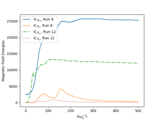
Figure 8: Axial and toroidal components of the magnetic field energy growth/saturation for different initial magnetic fields. Run 8 is for the initial toroidal magnetic field: $(b_{0},\gamma_{0})=(0.01,1.16)$. Runs 12 is for the initial axial magnetic field: $(b_{z0},\gamma_{0})=(0.01,1.16)$.

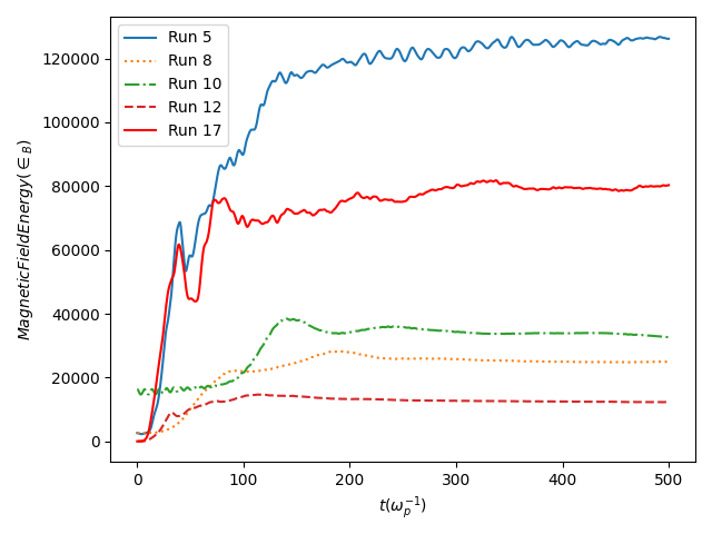
Figure 9: Magnetic field energy growth/saturation for different initial magnetic fields and jet velocities. Runs 5, 8, and 10 are for toroidal field: $(b_{0},\gamma_{0})=(0.01,2.3),(0.01,1.16),(0.025,1.16)$. Runs 12, 13, and 17 are for axial field: $(b_{0},\gamma_{0})=(0.01,1.16),(0.025,1.16),(0.01,2.3)$. The evolution of Run 13 is almost the same as that of Run 12, so it is not shown.

References

- Gabuzda (2019a) D. Gabuzda, “Evidence for helical magnetic fields associated with agn jets and the action of a cosmic battery,” galaxies 7, 1–14 (2019a).
- Weibel (1959) E. S. Weibel, “Spontaneously growing transverse waves in a plasma due to an anisotropic velocity distribution,” Phys. Rev. Lett. 2, 83–84 (1959).
- Fujita, Kato, and Okabe (2006) Y. Fujita, T. N. Kato, and N. Okabe, “Magnetic field generation by the weibel instability at temperature gradients in collisionless plasmas,” POP 13, 122901 (2006).
- Rieger and Duffy (2021) F. Rieger and P. Duffy, “Particle acceleration in shearing flows: Efficiencies and limits,” Astrophys. J. Lett. 886, 26 (2021).
- Meli and i. Nishikawa (2021) A. Meli and K. i. Nishikawa, “Particle-in-cell simulations of astrophysical relativistic jets,” Universe 7, 450 (2021).
- Alves, Zrake, and Fiuza (2018) E. P. Alves, J. Zrake, and F. Fiuza, “Efficient nonthermal particle acceleration by the kink instability in relativistic jets,” Phys. Rev. Lett. 121, 245101 (2018).
- Kato (2005) T. N. Kato, “Saturation mechanism of the weibel instability in weakly magnetized plasmas,” Physics of Plasma 12, 080705 (2005).
- Nishikawa et al. (2021) K. I. Nishikawa, I. Dutan, C. Köhn, and Y. Mizuno, “Pic methods in astrophysics: Simulations of relativistic jets and kinetic physics in astrophysical systems,” Living Rev. Comput. Astrophys. 7, 1 (2021).
- Kawashima et al. (2022) T. Kawashima, S. Ishiguro, T. Moritaka, R. Horiuchi, and K. Tomisaka, “Mushroom-instability-driven magnetic reconnections in collisionless relativistic jets,” APJ 928, 080705 (2022).
- Alves et al. (2014) E. P. Alves, T. Grismayer, R. A. Fonseca, and L. O. Silva, “Electron-scale shear instabilities: magnetic field generation and particle acceleration in astrophysical jets,” New J. Phys. 16, 035007 (2014).
- Hada et al. (2011) K. Hada, A. Doi, M. Kino, H. Nagai, Y. Hagiwara, and N. Kawaguchi, “An origin of the radio jet in m87 at the location of the central black hole,” Nature 477, 185–187 (2011).
- Alves et al. (2015) E. P. Alves, T. Grismayer, L. O. Silva, and R. A. Fonseca, “Transverse electron-scale instability in relativistic shear flows,” Phys. Rev. E 92, 021101(R) (2015).
- Ma et al. (2020) H. H. Ma, S. M. Weng, P. Li, X. F. Li, Y. X. Wang, S. H. Yew, M. Chen, P. McKenna, and Z. M. Sheng, “Growth, saturation, and collapse of laser-driven plasma density gratings,” Physics of Plasma 27, 073105 (2020).
- Begelman and Cioffi (1989) M. C. Begelman and D. F. Cioffi, “Overpressured cocoons in extragalactic radio sources,” APJL 345, L21 (1989).
- Gourgouliatos and Komissarov (2018) K. N. Gourgouliatos and S. Komissarov, “Reconfinement and loss of stability in jets from active galactic nuclei,” Nature Astronomy 2, 167–171 (2018).
- Mizuno et al. (2015) Y. Mizuno, J. L. Gomez, K.-I. Nishikawa, A. Meli, P. E. Hardee, and L. Rezzolla, “Recollimation shocks in magnetized relativistic jets,” APJ 809, 28 (2015).
- Gabuzda (2019b) D. Gabuzda, “The origin and structure of the magnetic fields and currents of agn jets,” galaxies 5, 1–11 (2019b).