Timed-Elastic-Band Based Variable Splitting for Autonomous Trajectory Planning

Abstract

Existing trajectory planning methods are struggling to handle the issue of autonomous track swinging during navigation, resulting in significant errors when reaching the destination. In this article, we address autonomous trajectory planning problems, which aims at developing innovative solutions to enhance the adaptability and robustness of unmanned systems in navigating complex and dynamic environments. We first introduce the variable splitting (VS) method as a constrained optimization method to reimagine the renowned Timed-Elastic-Band (TEB) algorithm, resulting in a novel collision avoidance approach named Timed-Elastic-Band based variable splitting (TEB-VS). The proposed TEB-VS demonstrates superior navigation stability, while maintaining nearly identical resource consumption to TEB. We then analyze the convergence of the proposed TEB-VS method. To evaluate the effectiveness and efficiency of TEB-VS, extensive experiments have been conducted using TurtleBot2 in both simulated environments and real-world datasets.

I Introduction

With the continuous advancement of machine learning technologies, various autonomous systems are becoming integral parts of human daily life, including autonomous driving vehicles, unmanned aerial vehicles, and robotic manipulators [1, 2, 3], among others. These systems contribute significantly to enhancing the efficiency of human activities, prompting extensive efforts to explore novel practical applications for autonomous technologies.

The traditional planning module in autonomous systems adopts a hierarchical structure, after map building with Simultaneous Localization and Mapping (SLAM) [4] or Visual simultaneous localization and mapping (VSLAM) [5], featuring both a global planner and a local planner. The global planner accumulates environmental information and provides a globally optimal path, typically at a slower frequency. In contrast, the local planner is responsible for quickly searching for an optimal trajectory that adheres to the global path. Well-known global planning methods, such as Dijkstra’s algorithm [6] and the A* algorithm [7], Jump Point Search algorithm [8], rapidly exploring random tree (RRT) algorithm [9], Informed-RRT* [10] and probability road map algorithm [11], are commonly employed for this purpose. In terms of local planning, Dynamic Window Approach (DWA) [12] and Timed-Elastic-Band (TEB) [13] can conceptualize the path planning problem as a multi-objective optimization problem. However, it turns out that when applied to non-convex optimization problems, the methods will remain computationally expensive.

Researchers have proposed various methods to enhance the performance of trajectory planning algorithms, particularly based on TEB and DWA algorithms. Examples of these enhanced approaches include the Improved Dynamic Window Approach (IDWA) introduced by Zhang et al. [14], Model Predictive Control with TEB (MPC-TEB) by Rosmann et al. [15], and egoTEB presented by Smith et al. [16]. It appears that one of the challenges is the difficulty in addressing the robot swing in the path, and the existing methods are not effectively mitigating this issue. Additionally, there seems to be a concern about accumulated errors during the movement process, leading to significant deviations from the intended trajectory, especially when reaching the endpoint.

Numerous optimization methods, such as Douglas-Rachford splitting (DRS) [17], Peaceman–Rachford splitting (PRS) [18], first-order primal-dual (FOPD) method [19], and alternating direction method of multipliers (ADMM)[20], leverage variable splitting and are well-suited for a range of constrained optimization problems. These techniques are particularly adept at transforming problems with inequality constraints into equivalent problems with equality constraints through variable splitting. In cases where inequality constraints are present, the solution of objective problems can be hard to directly compute.

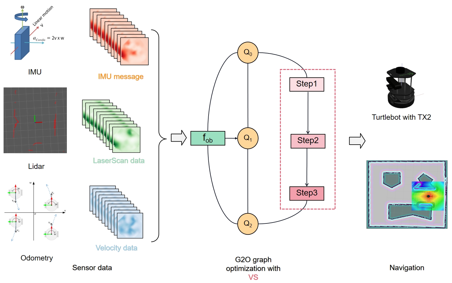
Figure 1: Our architecture: i) Real-time dynamic robot state information $Q_{i}$ is acquired from sensors, encompassing variables such as position, orientation, and other pertinent data. ii) In the method, the objective function is introduced as a new edge in the graph, replacing the original constraint. This step is pivotal for assimilating the results of the optimization process back into the overall trajectory planning framework. Steps 1-3 correspond to formulas (5a), (5b), and (5c)). iii) General Graph Optimization (G2O) [21] is employed to solve the subproblem arising in VS framework, where each vertex in the graph model denotes as a state, and edges represent objective functions. iv) The output of TEB-VS is the optimized trajectory for the robot.

In this article, we present a Timed-Elastic-Band based variable splitting (TEB-VS) method for solving autonomous trajectory planning problems. TEB-VS is highly effective for decomposing the global constrained optimization problem into several small constrained optimization problems, which has the superiority of computation time efficiency. The method is designed to be highly effective in decomposing the global constrained optimization problem into a series of local small constrained optimization problems. We also establish the convergence analysis of the TEB-VS method under mild assumptions. To assess the effectiveness and efficiency of TEB-VS, we apply the TEB-VS method to real-world datasets. The overall architecture is illustrated in Fig. 1.

II Problem Formulation

We consider general TEB sequences of $I$ robot configurations as

$$\begin{split}\Theta=\{\mathbf{x}_{0},(\mathbf{x}_{i},\Delta T_{i})\},\,i=1,\ldots,I.\end{split}$$ (1)

Here, $\Delta T_{i}$ represents the time interval, $\mathbf{x}_{i}=[x_{i},y_{i},\beta_{i}]^{\top}$ denotes the configuration of the robot pose, and $\mathbf{x}_{0}$ is an initial parameter. $x_{i}$, $y_{i}$, and $\beta_{i}$ represent the $x$-directional position, the $y$-directional position, and the orientation of the robot in the map coordinate system, respectively. In each time interval, the robot transitions from the current configuration to the next configuration in the TEB sequence $\Theta$. The primary objective is to derive the optimal TEB sequence $\Theta^{\star}$ as the trajectory.

Let $f_{i}(\Theta_{i})$ be defined as the function associated with each robot configuration $\Theta_{i}\in\Theta$. Given a set of robot configurations $\{\mathbf{x}_{i}\}_{i=0}^{I}$ and corresponding time intervals $\{\Delta T_{i}\}_{i=1}^{I}$, our objective is to perform constrained optimization.

$$\begin{split}\min_{\Theta}&F(\Theta)\\ {\mathrm{s.t.}}\ &\mathbf{c}_{k}\big{(}\mathbf{x}_{0},\mathbf{x}_{1},\ldots,\mathbf{x}_{I}\big{)}=\mathbf{0},\,k=1,\ldots,K,\\ &\mathbf{p}_{j}\big{(}\mathbf{x}_{0},\mathbf{x}_{1},\ldots,\mathbf{x}_{I}\big{)}\leq\mathbf{0},\,j=1,\ldots,J,\end{split}$$ (2)

where $F(\Theta)=\sum\gamma_{i}f_{i}(\Theta_{i})$ represents the cost function, and $\gamma_{i}$ serves as the weight for each function $f_{i}(\Theta_{i})$. The parameters $K$ and $J$ denote the number of equality and inequality constraint functions, respectively, and $\mathbf{c}_{k}$, $\mathbf{p}_{j}$ represent constraint functions—such as approximating turning radius, enforcing maximum velocities, maximum accelerations, and minimum obstacle separation.

Solving the problem (2) presents a greater challenge compared to the conventional TEB problem, as the constraint functions in (2) are nonconvex. In this following, we begin by establishing the framework of the proposed TEB-VS method.

III Methodology

In this section, we first introduce the framework of the proposed TEB-VS optimization method, and then derive the augmented TEB algorithm for solving the subproblems arising within the steps of the method. Under mild conditions, we also give the convergence analysis of the method.

III-A The General Framework

In this section, we exploit auxiliary variables to split the complex components, and introduce a barrier function $I(\mathbf{v})$ to replace the inequality constrained function. We can rewrite (2) as an equality constrained minimization problem

$$\begin{split}\begin{aligned} \min_{\Theta}&F(\Theta),\\ {\mathrm{s.t.}}\ &\mathbf{c}_{k}\big{(}\mathbf{x}_{0},\mathbf{x}_{1},\ldots,\mathbf{x}_{I}\big{)}=\mathbf{0},\,k=1,\ldots,K,\\ &\mathbf{p}_{j}\big{(}\mathbf{x}_{0},\mathbf{x}_{1},\ldots,\mathbf{x}_{I}\big{)}+\mathbf{v}_{j}=\mathbf{0},\,j=1,\ldots,J.\\ &I(\mathbf{v}_{j})=\begin{cases}0,&\mathbf{v}\geq 0,\\ \infty,&\text{otherwise}.\end{cases}\end{aligned}\end{split}$$ (3)

For simplifying the notation, we define the states $\mathbf{x}=\{\mathbf{x}_{1},\ldots,\mathbf{x}_{I}\}$, $\mathbf{v}=\{\mathbf{v}_{1},\ldots,\mathbf{v}_{J}\}$, and Lagrangian multipliers $\bm{\eta}=\{\bm{\eta}_{1},\ldots,\bm{\eta}_{J}\}$, $\bm{\zeta}=\{\bm{\zeta}_{1},\ldots,\bm{\zeta}_{K}\}$. The augmented Lagrangian function is then defined as

$$\begin{split}\begin{aligned} &\mathcal{L}(\mathbf{x},\mathbf{v};\bm{\eta},\bm{\zeta})=\sum_{i=1}^{I}\gamma_{i}f_{i}(\Theta_{i})+\sum_{j=1}^{J}\bm{\eta}_{j}^{\top}(\mathbf{p}_{j}(\mathbf{x})+\mathbf{v})\\ &+\sum_{j=1}^{J}\frac{\rho}{2}\|\mathbf{p}_{j}(\mathbf{x})+\mathbf{v}\|^{2}+\sum_{k=1}^{K}\bm{\zeta}_{k}^{\top}(\mathbf{c}_{k}(\mathbf{x}))+\sum_{k=1}^{K}\frac{\gamma}{2}\|\mathbf{c}_{k}(\mathbf{x})\|^{2},\end{aligned}\end{split}$$ (4)

where $\rho$, $\gamma$ are penalty parameters with the constraints, respectively. At each iteration, we can write

$$\mathbf{x}^{(n+1)} =\mathop{\arg\min}_{\mathbf{x}}\mathcal{L}(\mathbf{x},\mathbf{v}^{(n)};\bm{\eta}^{(n)},\bm{\zeta}^{(n)}),$$ (5a)

$$\mathbf{v}^{(n+1)} =\mathop{\arg\min}_{\mathbf{v}}\mathcal{L}(\mathbf{x}^{(n+1)},\mathbf{v};\bm{\eta}^{(n)},\bm{\zeta}^{(n)}),$$ (5b)

$$\bm{\eta}_{j}^{(n+1)} =\bm{\eta}_{j}^{(n)}+\rho(\mathbf{p}_{j}(\mathbf{x}^{(n+1)})+\mathbf{v}^{(n+1)}),$$ (5c)

$$\bm{\zeta}_{k}^{(n+1)} =\bm{\zeta}_{k}^{(n)}+\gamma\mathbf{c}_{k}(\mathbf{x}^{(n+1)}),$$ (5d)

where $n$ is the iteration number. In the objective function (2), acceleration and velocity optimization is one of the applications of Lagrangian Splitting. The velocity and acceleration can be minimax limits on velocity and acceleration. For the dual variable $\mathbf{v}$, the solution in (5b) can be computed by by

$$\mathbf{v}_{j}^{(n+1)} ={\max}\left(\mathbf{0},\,-\mathbf{p}_{j}(\mathbf{x}^{(n+1)})-\bm{\eta}_{j}^{(n)}/\rho\right).$$ (6)

The primal function (5a) is non-convex and lacks a closed-form solution. Consequently, we employ the augmented TEB method to address this challenge in the following.

III-B Augmented TEB for Solving $\mathbf{x}$-subproblem

In this section, we propose the augmented TEB algorithm for solving the $\mathbf{x}$-subproblem arising in the VS framework. Typically we have the objective function

$$\begin{split}\begin{aligned} &\mathbf{x}=\mathop{\arg\min}_{\mathbf{x}}\sum_{i=1}^{I}\gamma_{i}f_{i}(\Theta_{i})\\ &+\sum_{j=1}^{J}\frac{\rho}{2}\left\|\mathbf{p}_{j}(\mathbf{x})+\mathbf{v}+\frac{\bm{\eta}_{j}}{\rho}\right\|^{2}+\sum_{k=1}^{K}\frac{\gamma}{2}\left\|\mathbf{c}_{k}(\mathbf{x})+\frac{\bm{\zeta}_{k}}{\gamma}\right\|^{2}.\end{aligned}\end{split}$$ (7)

The problem of optimizing $\{(\mathbf{x}_{1},\Delta T_{1}),\ldots,(\mathbf{x}_{I},\Delta T_{I})\}$ can be addressed by constructing the G2O hypergraph [13, 21]. Utilizing a large-scale sparse matrix, the G2O serves as the optimization model. As depicted in Fig.1, the components of time $\{\Delta T_{i}\}$ and configuration are treated as nodes, while objective functions act as edges. The combination of nodes and edges forms the hypergraph. In the augmented TEB method, the classical constraint edges are transformed into objective functions using variable splitting. This process involves representing the edges from traditional constraints to objective functions with variable splitting techniques. The optimized edges and vertices resulting from this transformation are then incorporated into the sparse optimizer. Subsequently, the sparse optimizer generates the corresponding results.

On the premise that the other input parameters of TEB are unchanged, replacing the speed constraint to (5) as edge. In a similar manner, the VS method can be applied to handle other constraints and objectives within the trajectory planning problem. For instance, if there are constraints related to waypoints, obstacles, and the fastest path, these can be reformulated and replaced using the VS method.

III-C Convergence Analysis

In this section, we establish the convergence analysis of the method. We first make the following assumptions.

Assumption A1.

The function $F(\mathbf{x})$ is strongly amenable at $\mathbf{x}$ and $F(\mathbf{x})$ is prox-regular [22]. That is, for any $\mathbf{x}_{a}$, $\mathbf{x}_{b}$ in a neighbourhood of $\mathbf{x}$, there exists $e_{x}>0$ such that

$$\begin{split}\begin{aligned} F(\mathbf{x}_{a})\geq F(\mathbf{x}_{b})-\frac{e_{x}}{2}\|\mathbf{x}_{a}-\mathbf{x}_{b}\|_{2}^{2}+\langle\partial F(\mathbf{x}),\mathbf{x}_{a}-\mathbf{x}_{b}\rangle.\end{aligned}\end{split}$$ (8)

Assumption A2.

The sequence $\{\mathbf{x}^{(n)}\}$ generated by the augmented TEB converges to a local minimum $\mathbf{x}^{\star}$.

We then prove that the sequence $\{\mathcal{L}(\mathbf{x}^{(n)},\mathbf{v}^{(n)},\bm{\eta}^{(n)},\bm{\zeta}^{(n)})\}$ generated by TEB-VS is monotonically non-increasing in the following lemma.

Lemma 1.

Let $\{\mathbf{x}^{(n)},\mathbf{v}^{(n)},\bm{\eta}^{(n)},\bm{\zeta}^{(n)}\}$ be the sequence. If $\rho e_{c}^{2}+\gamma e_{p}^{2}>e_{x}$, and the Jacobian $\mathbf{J}_{c}$, and $\mathbf{J}_{p}$ have full-column rank with

$$\begin{split}\mathbf{\mathbf{J}}_{c}^{\top}\mathbf{\mathbf{J}}_{c}\succeq e_{c}^{2}\mathbf{I},\,\mathbf{\mathbf{J}}_{p}^{\top}\mathbf{\mathbf{J}}_{p}\succeq e_{p}^{2}\mathbf{I},\quad e_{c},e_{p}>0,\end{split}$$ (9)

Then, the sequence $\{\mathbf{x}^{(n)},\mathbf{v}^{(n)},\bm{\eta}^{(n)},\bm{\zeta}^{(n)}\}$ is nonincreasing with the iteration number $n$.

Proof.

For the $\bm{\zeta}$-subproblem, we obtain

$$\begin{split}\begin{aligned} &\mathcal{L}(\mathbf{x}^{(n+1)},\mathbf{v}^{(n+1)};\bm{\eta}^{(n+1)},\bm{\zeta}^{(n+1)})-\\ &\quad\mathcal{L}(\mathbf{x}^{(n+1)},\mathbf{v}^{(n+1)};\bm{\eta}^{(n+1)},\bm{\zeta}^{(n)})\\ &=\frac{1}{\gamma}\|\bm{\zeta}^{(n+1)}-\bm{\zeta}^{(n)}\|^{2}.\end{aligned}\end{split}$$ (10)

Similar to the $\bm{\eta}$-subproblem, we obtain

$$\begin{split}\begin{aligned} &\mathcal{L}(\mathbf{x}^{(n+1)},\!\mathbf{v}^{(n+1)};\!\bm{\eta}^{(n+1)},\!\bm{\zeta}^{(n)})\!-\!\mathcal{L}(\mathbf{x}^{(n+1)},\!\mathbf{v}^{(n+1)};\!\bm{\eta}^{(n)},\!\bm{\zeta}^{(n)})\\ &=\langle\bm{\eta}^{(n+1)},\mathbf{c}(\mathbf{x}^{(n)})+\mathbf{v}\rangle-\langle\bm{\eta}^{(n)},\mathbf{c}(\mathbf{x}^{(n)})+\mathbf{v}\rangle\\ &=\frac{1}{\rho}\|\bm{\eta}^{(n+1)}-\bm{\eta}^{(n)}\|^{2}.\end{aligned}\end{split}$$ (11)

We set $F(\mathbf{x})=\sum_{i=1}^{I}F(\mathbf{x}_{i},\Delta T_{i})$. For the $\mathbf{x}$-subproblem in (5a), we can obtain

$$\begin{split}&\mathcal{L}(\mathbf{x}^{(n)},\mathbf{v}^{(n)};\bm{\eta}^{(n)},\bm{\zeta}^{(n)})-\mathcal{L}(\mathbf{x}^{(n+1)},\mathbf{v}^{(n)};\bm{\eta}^{(n)},\bm{\zeta}^{(n)})\\ &=F(\mathbf{x}^{(n)})+\langle\bm{\eta}^{(n)},\mathbf{v}^{(n)}+\mathbf{c}(\mathbf{x}^{(n)})\rangle+\frac{\rho}{2}\|\mathbf{v}^{(n)}+\mathbf{c}(\mathbf{x}^{(n+1)})\|^{2}\\ &\,+\langle\bm{\zeta}^{(n)},\mathbf{p}(\mathbf{x}^{(n)})\rangle+\frac{\gamma}{2}\|\mathbf{p}(\mathbf{x}^{(n+1)})\|^{2}-\theta(\mathbf{x}^{(n+1)})\\ &\quad-\langle\bm{\eta}^{(n)},\mathbf{v}^{(n)}+\mathbf{c}(\mathbf{x}^{(n+1)})\rangle-\frac{\rho}{2}\|\mathbf{v}^{(n)}+\mathbf{c}(\mathbf{x}^{(n+1)})\|^{2}\\ &\qquad-\langle\bm{\zeta}^{(n)},\mathbf{p}(\mathbf{x}^{(n+1)})\rangle-\frac{\gamma}{2}\|\mathbf{p}(\mathbf{x}^{(n+1)})\|^{2}\\ &=F(\mathbf{x}^{(n)})+\langle\bm{\eta}^{(n)},\mathbf{c}(\mathbf{x}^{(n)})-\mathbf{c}(\mathbf{x}^{(n+1)})\rangle-F(\mathbf{x}^{(n+1)})\\ &\,+\rho\langle\mathbf{c}(\mathbf{x}^{(n+1)})+\mathbf{v}^{(n)},\mathbf{c}(\mathbf{x}^{(n+1)})-\mathbf{c}(\mathbf{x}^{(n)})\rangle\\ &\quad+\frac{\rho}{2}\|\mathbf{c}(\mathbf{x}^{(n+1)})-\mathbf{c}(\mathbf{x}^{(n)})\|^{2}+\frac{\gamma}{2}\|\mathbf{p}(\mathbf{x}^{(n+1)})-\mathbf{p}(\mathbf{x}^{(n)})\|^{2}\\ &\,\quad+\gamma\langle\mathbf{p}(\mathbf{x}^{(n+1)}),\mathbf{p}(\mathbf{x}^{(n+1)})-\mathbf{p}(\mathbf{x}^{(n)})\rangle\\ &\qquad+\langle\bm{\zeta}^{(n)},\mathbf{p}(\mathbf{x}^{(n)}-\mathbf{p}(\mathbf{x}^{(n+1)})\rangle\\ &>F(\mathbf{x}^{(n)})-F(\mathbf{x}^{(n+1)})\\ &\,+\langle\bm{\eta}^{(n)}+\rho(\mathbf{c}(\mathbf{x}^{(n+1)})+\mathbf{v}^{(n)}),\mathbf{J}_{c}^{\top}(\mathbf{x}^{(n)}-\mathbf{x}^{(n+1)})\rangle\\ &\quad+\langle\bm{\zeta}^{(n)}+\gamma(\mathbf{p}(\mathbf{x}^{(n+1)})),\mathbf{J}_{p}^{\top}(\mathbf{x}^{(n+1)}-\mathbf{x}^{(n)})\rangle\\ &\quad+\frac{\rho}{2}\mathbf{J}_{c}^{\top}\mathbf{J}_{c}\|\mathbf{x}^{(n+1)})-\mathbf{x}^{(n)}\|^{2}+\frac{\gamma}{2}\mathbf{J}_{p}^{\top}\mathbf{J}_{p}\|\mathbf{x}^{(n+1)})-\mathbf{x}^{(n)}\|^{2}\\ &{\geq}-\frac{e_{x}}{2}\|\mathbf{x}^{(n)}-\mathbf{x}^{(n+1)}\|^{2}++\frac{\rho e_{c}}{2}\|\mathbf{x}^{(n+1)}-\mathbf{x}^{(n)}\|^{2}\\ &\quad+\frac{\gamma\kappa_{e}}{2}\|\mathbf{x}^{(n+1)}-\mathbf{x}^{(n)}\|^{2}\\ &{\geq}\left(\frac{\rho e_{c}^{2}}{2}+\frac{\gamma e_{p}^{2}}{2}-\frac{e_{x}}{2}\right)\|\mathbf{x}^{(n+1)}-\mathbf{x}^{(n)}\|^{2},\end{split}$$ (12)

and by combining (12), (10), and (11), we get

$$\begin{split}\begin{aligned} &\mathcal{L}(\mathbf{x}^{(n+1)},\mathbf{v}^{(n+1)};\bm{\eta}^{(n+1)},\bm{\zeta}^{(n+1)})-\mathcal{L}(\mathbf{x}^{(n)},\mathbf{v}^{(n)};\bm{\eta}^{(n)},\bm{\zeta}^{(n)})\\ &\leq\frac{e_{x}-\rho_{1}e_{c}^{2}-\gamma e_{p}^{2}}{2}\|\mathbf{x}^{(n+1)}-\mathbf{x}^{(n)}\|^{2}+\frac{1}{\rho}\|\bm{\eta}^{(n+1)}-\bm{\eta}^{(n)}\|^{2}\\ &\quad+\frac{1}{\gamma}\|\bm{\zeta}^{(n+1)}-\bm{\zeta}^{(n)}\|^{2},\end{aligned}\end{split}$$ (13)

which will be nonnegative provided that $\rho e_{c}^{2}+\gamma e_{p}^{2}>e_{x}$. Thus, we get the results.   

Based on Lemma 1, Assumptions A1 and A2, we now give the convergence analysis by TEB-VS in the following theorem.

Theorem 1 (Convergence of TEB-VS).

Let Assumptions A1 and A2 be satisfied. Then, the sequence $\{\mathbf{x}^{(n)},\mathbf{v}^{(n)},\bm{\eta}^{(n)},\bm{\zeta}^{(n)}\}$ generated by TEB-VS converges to a local minimum $(\mathbf{x}^{\star},\mathbf{v}^{\star},\bm{\eta}^{\star},\bm{\zeta}^{\star})$.

Proof.

By Lemma 1, the sequence $\mathcal{L}(\mathbf{x}^{(n)},\mathbf{v}^{(n)};\bm{\eta}^{(n)},\bm{\zeta}^{(n)})$ is nonincreasing. Since $\mathcal{L}(\mathbf{x}^{(n)},\mathbf{v}^{(n)};\bm{\eta}^{(n)},\bm{\zeta}^{(n)})$ is upper bounded by $\mathcal{L}(\mathbf{x}^{(0)},\mathbf{v}^{(0)};\bm{\eta}^{(0)},\bm{\zeta}^{(0)})$, and lower bounded by $F(\mathbf{x}^{(n)})$. There exists a local minimum $\mathbf{x}^{\star}$ such that the sequence ${\mathbf{x}^{(i)}}$ converges to $\mathbf{x}_{1:T}^{\star}$. The $\mathbf{v}_{1:T}$ subproblem has a unique minimum $\mathbf{v}^{\star}$ [20]. We then deduce that the sequence $\{\mathbf{x}^{(n)},\mathbf{v}^{(n)},\bm{\eta}^{(n)},\bm{\zeta}^{(n)}\}$ converges to $(\mathbf{x}^{\star},\mathbf{v}^{\star},\bm{\eta}^{\star},\bm{\zeta}^{\star})$. We deduce the sequence $\{\mathbf{x}^{(n)},\mathbf{v}^{(n)},\bm{\eta}^{(n)},\bm{\zeta}^{(n)}\}$ generated by TEB-VS is locally convergent to $(\mathbf{x}^{\star},\mathbf{v}^{\star},\bm{\eta}^{\star},\bm{\zeta}^{\star})$.   

IV Experiment Results

In this section, we assess the performance of the proposed algorithm through simulated data and real-life trajectory planning applications. First, we introduce the algorithm and present simulation results. Next, we illustrate the practical application of the algorithm in real robots. The results are presented and analyzed in both contexts. As depicted in Fig.1, in addition to the Turtlebot2 robot chassis, which includes odometry and an inertial measurement unit (IMU), radar sensors have been incorporated to determine obstacle distances. All relevant parameters and target equations are input into the G2O framework for graph optimization, and the optimized velocity is then output to odometry to govern the robot’s movement.

IV-A Experimental Settings

Utilizing the Gazebo simulator on the Robot Operating System (ROS) platform, we construct a robot model that precisely mirrors the physical robot. All simulation experiments are conducted on Ubuntu 16.04 operating system. Initially, the model world is established using Gazebo, and subsequently, the SLAM method is employed to map this model world in Fig.2. Following the creation of the Octomap [23], three methods including DWA, TEB, and TEB-VS are individually applied for autonomous trajectory planning.

TABLE I: Velocity variation values generated by different methods

Process Velocity	Algorithm	Mean Value	Standard Deviation	Variance
	DWA	0.07790	0.05297	0.00281
Angular velocity variation in rotation	TEB	0.02431	0.04271	0.00182
	TEB-VS	0.05018	0.09003	0.0081
	DWA	0.00833	0.01887	3.56123$\times 10^{-4}$
Linear velocity variation in rotation	TEB	0.00753	0.02420	$5.85836\times 10^{-4}$
	TEB-VS	0.01115	0.02067	$4.27124\times 10^{-4}$
	DWA	0.02523	0.02746	$7.54212\times 10^{-4}$
Angular velocity variation in linear motion	TEB	0.02620	0.01483	$2.19787\times 10^{-4}$
	TEB-VS	0.01788	0.00988	9.76143$\times 10^{-5}$
	DWA	0.00417	0.01594	$2.54073\times 10^{-4}$
Linear velocity variation in linear motion	TEB	$2.58556\times 10^{-4}$	$3.6577\times 10^{-4}$	$1.33788\times 10^{-7}$
	TEB-VS	2.33244$\times 10^{-4}$	3.27672$\times 10^{-4}$	1.07369$\times 10^{-7}$

As the robot operates within a two-dimensional plane, its motion is systematically divided into two key components: linear motion and rotation. In terms of stability, particular emphasis is placed on monitoring the linear velocity and angular velocity between two consecutive configurations, whether the robot is moving in a straight line or rotating. This focus ensures a robust and stable autonomous trajectory planning process. The robot follows a trajectory from the left side of the map to the right side. Throughout this journey, its orientation undergoes a transformation from the left direction of the starting point to the right direction, providing a visual representation of the autonomous trajectory planning process. The trajectories generated by three distinct algorithms, all originating from the same starting point and concluding at the same endpoint.

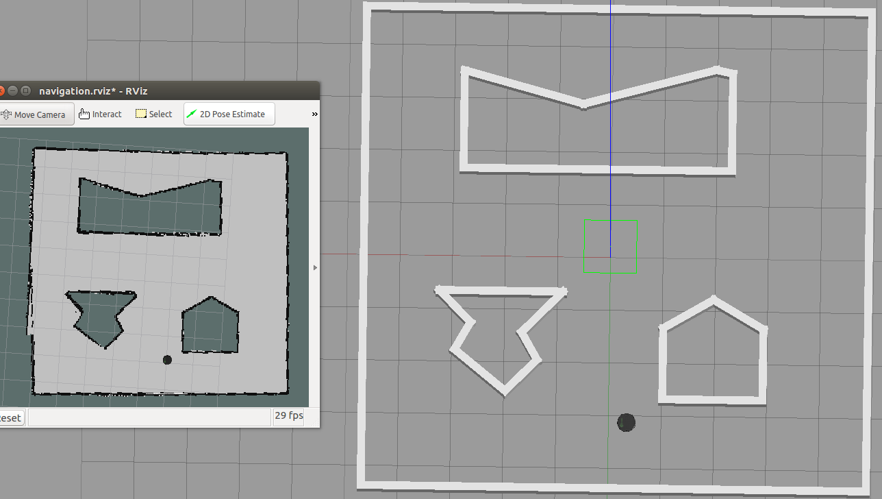
Figure 2: Gazebo world, the right part of this figure shows the simulation room by gazebo and the left part is OctoMap [23] based on this room. The black point is robot Turtlebot2. The details will also be updated on the map in real time when robot navigation in this room.

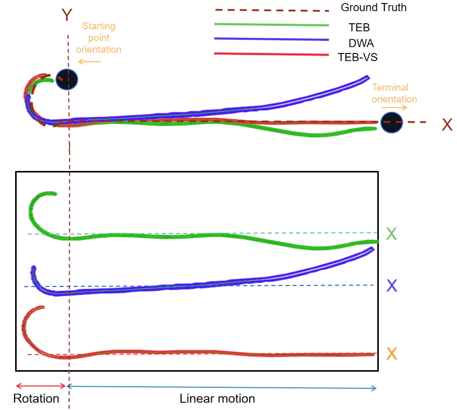
Figure 3: Autonomous trajectory planning generated by different methods. The starting point is at coordinates (2,5) with a specific orientation, and the goal is to navigate coordinates (9,5) with a different orientation in the OctoMap. There are two phases of autonomous trajectory planning motion: rotation and linear motion. The dotted lines are the ground truth. When comparing velocity stability, especially in the context of navigating the robot, it is important to distinguish between the rotational and linear processes. Special attention should be given to the left and right swing of the robot during the linear motion phase, as this significantly impact the accuracy of reaching the endpoint.

IV-B Simulation Results

We demonstrate the autonomous trajectory planning results generated by different methods in Fig.3. The method outperforms the other algorithms in terms of trajectory planning accuracy, resulting in a markedly superior trajectory. Additionally, the motion of the robot following the method exhibits smoother operation throughout the autonomous trajectory planning process.

Table I illustrates the velocity variation results. The comprehensive comparison of velocity stability shows that the TEB-VS method outperforms both TEB and DWA methods. During the linear motion, the comparative analysis between the TEB-VS and TEB methods reveals that the angular velocity variation in the rotation phase is notably greater for the proposed method. TEB-VS exhibits significantly better angular velocity variation compared to both TEB and DWA, achieving optimizations of over $46.5\%$ and $41.1\%$, respectively. Additionally, the standard deviation and variance of TEB-VS are smaller than those of TEB, indicating enhanced stability in linear motion.

In addition to comparing the running trajectories, we conducted a comparative analysis of the algorithm’s runtime performance and the robot’s trajectory planning speed. Table II presents the running time results for DWA, TEB and TEB-VS methods. Notably, given that the typical sampling frequency of the robot is generally around $1-20$Hz, the operation time for three methods remains significantly shorter than the sampling frequency. As a result, the impact on the robot’s operational efficiency is minimal.

TABLE II: Running time of simulation

Method	Running time(s)
DWA	0.00057971
TEB	0.00057971
TEB-VS	0.00171429

IV-C Real-Life Robot Results

Similar to the simulation results, comparative tests on running time and velocity variation of the robots affirm that the method’s running time is negligible, and the introduction of additional iterations has minimal impact on the algorithm’s performance. In testing the actual speed change of the Turtlebot2 robot, we observed that the stability optimization result during linear motion decreased from 46.5% in simulation to 26.7%. Despite this reduction, the outcome remains superior to that of TEB, confirming the efficacy of the method in real-world scenarios.

V Conclusion

In this article, we present the new Timed-Elastic-Band based variable splitting (TEB-VS) method to solve autonomous trajectory planning problems. We also establish the convergence of the proposed method. Through extensive experiments with a real robot, our algorithm demonstrates superior effectiveness compared to the other classical methods. The TEB-VS method exhibits a 46.5% increase in speed stability in simulation and a 26.7% increase in real-life robot experiments. Our future focus will delve into further optimizations, particularly in the realm of fastest path or trajectory optimization.

References

- [1] H. H. Kang and C. K. Ahn, “Two-stage iterative finite-memory neural network identification for unmanned aerial vehicles,” IEEE Trans. Circuits Syst. II Express Briefs, In Press, 2023.
- [2] M. Zhang, Z. Zhang, and M. Sun, “Adaptive tracking control of uncertain robotic manipulators,” IEEE Trans. Circuits Syst. II Express Briefs, 2024.
- [3] R. Gao, S. Särkkä, R. Claveria-Vega, and S. Godsill, “Autonomous tracking and state estimation with generalised group Lasso,” IEEE Trans. Cybern., vol. 52, no. 11, pp. 12 056–12 070, June 2021.
- [4] Y. Tan, H. Deng, M. Sun, M. Zhou, Y. Chen, L. Chen, C. Wang, and F. An, “A reconfigurable coprocessor for simultaneous localization and mapping algorithms in fpga,” IEEE Trans. Circuits Syst. II Express Briefs, vol. 70, no. 1, pp. 286–290, 2022.
- [5] Y. Liu, K. Huang, N. Zhao, J. Li, S. Hao, Z. Huang, X. Qi, X. Wang, L. Zhou, L. Chang, et al., “BOHA: A high performance VSLAM backend optimization hardware accelerator using recursive fine-grain H-matrix decomposition and early-computing with approximate linear solver,” IEEE Trans. Circuits Syst. II Express Briefs, In Press, 2023.
- [6] E. W. Dijkstra, “A note on two problems in connection with graphs,” Numer. Math., pp. 287–290, 1959.
- [7] P. E. Hart, N. J. Nilsson, and B. Raphael, “A formal basis for the heuristic determination of minimum cost paths,” IEEE Trans. Syst. Man Cybern. Syst., vol. 4, no. 2, pp. 100–107, 1968.
- [8] F. Duchoň, A. Babinec, M. Kajan, P. Beňo, M. Florek, T. Fico, and L. Jurišica, “Path planning with modified a star algorithm for a mobile robot,” Procedia Eng., vol. 96, pp. 59–69, 2014.
- [9] S. M. LaValle, J. J. Kuffner, B. Donald, et al., “Rapidly-exploring random trees: Progress and prospects,” Algorithmic and Comput. robotics: new directions, vol. 5, pp. 293–308, 2001.
- [10] J. D. Gammell, S. S. Srinivasa, and T. D. Barfoot, “Informed rrt*: Optimal sampling-based path planning focused via direct sampling of an admissible ellipsoidal heuristic,” in 2014 IEEE/RSJ International Conference on Intelligent Robots and Systems, 2014, pp. 2997–3004.
- [11] T. Siméon, J.-P. Laumond, and C. Nissoux, “Visibility-based probabilistic roadmaps for motion planning,” Adv. Robotics, vol. 14, no. 6, pp. 477–493, 2000.
- [12] D. Fox, W. Burgard, and S. Thrun, “The dynamic window approach to collision avoidance,” IEEE Robot. Autom. Mag., vol. 4, no. 1, pp. 23–33, 1997.
- [13] C. Rösmann, W. Feiten, T. Wösch, F. Hoffmann, and T. Bertram, “Trajectory modification considering dynamic constraints of autonomous robots,” in Proc. 7th German Conference on Robotics. VDE, 2012, pp. 1–6.
- [14] H. Zhang, L. Dou, H. Fang, and J. Chen, “Autonomous indoor exploration of mobile robots based on door-guidance and improved dynamic window approach,” in Proc. IEEE International Conference on Robotics and Biomimetics. IEEE, 2009, pp. 408–413.
- [15] C. Rösmann, F. Hoffmann, and T. Bertram, “Timed-elastic-bands for time-optimal point-to-point nonlinear model predictive control,” in Proc. European Control Conference. IEEE, 2015, pp. 3352–3357.
- [16] J. S. Smith, R. Xu, and P. Vela, “EGOTEB: Egocentric, perception space navigation using timed-elastic-bands,” in Proc. IEEE International Conference on Robotics and Automation. IEEE, 2020, pp. 2703–2709.
- [17] J. Eckstein and D. Bertsekas, “On the Douglas-Rachford splitting method and the proximal point algorithm for maximal monotone operators,” Math. Programming, vol. 55, pp. 293–318, 1992.
- [18] D. W. Peaceman and H. H. Rachford, “The numerical solution of parabolic and elliptic differential equations,” J. Soc. Indust. Appl. Math., vol. 3, no. 1, pp. 28–41, 1955.
- [19] A. Chambolle and T. Pock, “A first-order primal-dual algorithm for convex problems with applications to imaging,” J. Math. Imaging. Vis., vol. 40, no. 1, pp. 120–145, May 2011.
- [20] S. Boyd, N. Parikh, E. Chu, B. Peleato, and J. Eckstein, “Distributed optimization and statistical learning via the alternating direction method of multipliers,” Foundations and Trends in Machine Learning., vol. 3, no. 1, pp. 1–122, 2011.
- [21] R. Kummerle, G. Grisetti, H. Strasdat, K. Konolige, and W. Burgard, “G2O: A general framework for graph optimization,” in Proc. IEEE International Conference on Robotics Automation, 2011, pp. 3607–3613.
- [22] R. T. Rockafellar and R. Wets, “Variational analysis,” Berlin, Germany: Springer Verlag, 1998.
- [23] A. Hornung, K. M. Wurm, M. Bennewitz, C. Stachniss, and W. Burgard, “Octomap: an efficient probabilistic 3D mapping framework based on octrees,” Springer US, no. 3, 2013.