Computing Augustin Information via
Hybrid Geodesically Convex Optimization

Abstract

We propose a Riemannian gradient descent with the Poincaré metric to compute the order-$\alpha$ Augustin information, a widely used quantity for characterizing exponential error behaviors in information theory. We prove that the algorithm converges to the optimum at a rate of $\mathcal{O}(1/T)$. As far as we know, this is the first algorithm with a non-asymptotic optimization error guarantee for all positive orders. Numerical experimental results demonstrate the empirical efficiency of the algorithm. Our result is based on a novel hybrid analysis of Riemannian gradient descent for functions that are geodesically convex in a Riemannian metric and geodesically smooth in another.

1 Introduction

Characterizing operational quantities of interest in terms of a single-letter information-theoretic quantity is fundamental to information theory. However, certain single-letter quantities involve an optimization that is not easy to solve. This work aims to propose an optimization framework for computing an essential family of information-theoretic quantities, termed the Augustin information [4, 5, 17, 43, 32, 13, 44, 11], with the first non-asymptotic optimization error guarantee.

Consider two probability distributions $P$ and $Q$ sharing the same finite alphabet $\mathcal{Y}$. The order-$\alpha$ Rényi divergence ($\alpha\in(0,\infty)\backslash\{1\}$) is defined as [39, 42]

$$D_{\alpha}(P\|Q):=\frac{1}{\alpha-1}\log\sum_{y\in\mathcal{Y}}P^{\alpha}(y)Q^{1-\alpha}(y).$$

As $\alpha$ tends to $1$, we have

$$\lim_{\alpha\to 1}D_{\alpha}(P\|Q)=D(P\|Q),$$

where $D(P\|Q):=\mathbb{E}_{Y\sim P}\left[\log\frac{P(Y)}{Q(Y)}\right]$ is the Kullback–Leibler (KL) divergence. The KL divergence defines Shannon’s mutual information for a prior distribution $P_{X}$ on the input alphabet $\mathcal{X}$ and a conditional distribution $P_{Y|X}$ as

$$I(P_{X},P_{Y|X}) :=\min_{Q_{Y}}\mathbb{E}_{X}D(P_{Y\mid X}(\cdot\mid X)\|Q_{Y})$$

$$=D(P_{Y\mid X}\|P_{Y}|P_{X}),$$

where the minimization is over all probability distributions on $\mathcal{Y}$ and $P_{Y}=\mathbb{E}_{X}[P_{Y|X}]$. Augustin generalized Shannon’s mutual information to the order-$\alpha$ Augustin information [4, 5], defined as

$$I_{\alpha}(P_{X},P_{Y|X}):=\min_{Q_{Y}}\mathbb{E}_{X}D_{\alpha}(P_{Y\mid X}(\cdot\mid X)\|Q_{Y}).$$ (1)

The Augustin information yields a wealth of applications in information theory, including:

1. characterizing the cut-off rate of channel coding [17],

2. determining the error exponent of optimal constant compositions codes for rates below Shannon’s capacity [22, 4, 7, 5, 18, 33, 19, 12],

3. determining the strong converse exponent of channel coding for rates above Shannon’s capacity [3, 35, 20, 30, 31],

4. determining the error exponent of variable-length data compression with side information [10, 14],

5. demonstrating an achievable secrecy exponent for privacy amplification and wiretap channel coding via regular random binning [29, 40].

In spite of the operational significance of the Augustin information, computing it is not an easy task. The order-$\alpha$ Augustin information does not have a closed-form expression in general unless $\alpha=1$. The optimization problem (1) is indeed convex [42, Theorem 12] so we may consider solving the optimization problem (1) via gradient descent. However, existing non-asymptotic analyses of gradient descent assume either Lipschitzness or smoothness of the objective function [9, 34, 26]. These two conditions, which we refer to as smoothness-type conditions, are violated by the optimization problem (1) [48].

In this paper, we adopt a geodesically convex optimization approach [49, 8, 45, 1]. This approach utilizes generalizations of convexity and smoothness-type conditions for Riemannian manifolds, namely geodesic convexity, geodesic Lipschitzness, and geodesic smoothness [49, 38, 41, 47, 50, 23, 24, 15, 2]. Since the lack of standard smoothness-type conditions is the main difficulty in applying gradient descent-type methods, we may find an appropriate Riemannian metric with respect to which the objective function in the optimization problem (1) is geodesically smooth.

Indeed, we have found that the objective function is geodesically smooth with respect to a Riemannian metric called the Poincaré metric. However, numerical experiments suggest that the objective function is geodesically non-convex under this metric. This poses another challenge. Existing analyses for Riemannian gradient descent, a direct extension of vanilla gradient descent, require both geodesic convexity and geodesic smoothness under the same Riemannian metric [49, 8].

Our main theoretical contribution lies in analyzing Riemannian gradient descent under a hybrid scenario, where the objective function is geodesically convex with respect to one Riemannian metric and geodesically smooth with respect to another. We prove that under this hybrid scenario, Riemannian gradient descent converges at a rate of $\mathcal{O}(1/T)$, identical to the rate of vanilla gradient descent under the Euclidean setup.

Given that the objective function for computing the Augustin information is convex under the standard Euclidean structure and geodesically smooth under the Poincaré metric, our proposed hybrid framework offers a viable approach to solve this problem. In particular, we prove that Riemannian gradient descent with the Poincaré metric converges at a rate of $\mathcal{O}(1/T)$ for computing the Augustin information. This marks the first algorithm for computing the Augustin information that has a non-asymptotic optimization error bound for all $\alpha>0$.

Due to the page limit, we defer the proofs of lemmas and theorems in this paper to the appendix.

Notations. We denote the all-ones vector by $\mathbbm{1}$. We denote the set of vectors with non-negative entries and strictly positive entries by $\mathbb{R}^{N}_{+}$ and $\mathbb{R}^{N}_{++}$, respectively. The $i$-th entry of $x$ is denoted by $x^{(i)}$. For any function $f:\mathbb{R}\to\mathbb{R}$ and vector $x$, we define $f(x)$ as the vector whose $i$-th entry equals $f(x^{(i)})$. Hence, for example, the $i$-th entry of $\exp(x)$ is $\exp x^{(i)}$. The probability simplex in $\mathbb{R}^{N}_{+}$ is denoted by $\Delta^{N}_{+}$, and the intersection of $\mathbb{R}^{N}_{++}$ and $\Delta^{N}_{+}$ is denoted by $\Delta^{N}_{++}$. The notations $\odot$ and $\oslash$ denote entry-wise product and entry-wise division, respectively. For $x,y\in\mathbb{R}^{N}$, the partial order $x\leq y$ means $y-x\in\mathbb{R}^{N}_{+}$. For a set $S\in\mathbb{R}^{N}$, the boundary of $S$ is denoted by $\partial S$. The set $\{1,2,\ldots,N\}$ is denoted by $[N]$.

2 Related Work

2.1 Computing the Augustin Information

Nakiboğlu [32] showed that the minimizer of the optimization problem (1) satisfies a fixed-point equation and proved that the associated fixed-point iteration converges to the order-$\alpha$ Augustin information for $\alpha\in(0,1)$. Li and Cevher [28] provided a line search gradient-based algorithm to solve optimization problems on the probability simplex, which can also be used to solve the optimization problem (1). You et al. [48] proposed a gradient-based method for minimizing quantum Rényi divergences, which includes the optimization problem (1) as a special case for all $\alpha>0$. These works only guarantee asymptotic convergence of the algorithms. Analysis of the convergence rate before the presen work is still missing.

2.2 Hybrid Analysis

Antonakopoulos et al. [2] considered (Euclidean) convex and geodesically Lipschitz objective functions, analyzing the regret rates of the follow-the-regularized-leader algorithm and online mirror descent. Weber and Sra [46] considered geodesically convex and (Euclidean) smooth objective functions, analyzing the optimization error of the convex-concave procedure. The former did not consider the hybrid case of geodesic convexity and geodesic smoothness under different Riemannian metrics. The latter only analyzed a special case of the hybrid scenario we proposed. Neither of them analyzed Riemannian gradient descent.

3 Preliminaries

This chapter introduces relevant concepts in geodesic convex optimization.

3.1 Smooth Convex Optimization

If an optimization problem is convex, we may consider using (projected) gradient descent to approximate a global minimizer. Existing non-asymptotic error bounds of gradient descent require the objective function to be either Lipschitz or smooth.

Definition 3.1.

We say a function $f:\mathbb{R}^{N}\to\mathbb{R}$ is $L$-Lipschitz for some $L>0$ if for any $x,y\in\mathbb{R}^{N}$, the function satisfies

$$|f(y)-f(x)|\leq L\|y-x\|_{2}.$$

We say a function $f:\mathbb{R}^{N}\to\mathbb{R}$ is $L$-smooth for some $L>0$ if for any $x,y\in\mathbb{R}^{N}$, the function satisfies

$$f(y)\leq f(x)+\langle\nabla f(x),y-x\rangle+\frac{L}{2}\|y-x\|_{2}^{2}.$$

Given a convex optimization problem $\min_{x\in C}f(x)$, gradient descent converges at a rate of $\mathcal{O}(1/\sqrt{T})$ for the Lipschitz case and $\mathcal{O}(1/T)$ for the smoothness case, where $T$ denotes the number of iterations. However, You et al. [48, Proposition III.1] showed that the objective function in the optimization problem (1) is neither Lipschitz nor smooth.

3.2 Basics of Riemannian Geometry

An $N$-dimensional topological manifold $\mathcal{M}$ is a topological space that is Hausdorff, second countable, and locally homeomorphic to $\mathbb{R}^{N}$. The tangent space at a point $x\in\mathcal{M}$, denoted as $T_{x}\mathcal{M}$, is the set of all vectors tangent to the manifold at $x$. A Riemannian metric $\mathfrak{g}$ on $\mathcal{M}$ defines an inner product on each tangent space. The inner product on $T_{x}\mathcal{M}$ is denoted as $\langle\cdot,\cdot\rangle_{x}$. A Riemannian manifold $(\mathcal{M},\mathfrak{g})$ is a topological manifold $\mathcal{M}$ equipped with a Riemannian metric $\mathfrak{g}$. Given a Riemannian metric, the induced norm of a tangent vector $v\in T_{x}\mathcal{M}$ is given by $\|v\|_{x}:=\sqrt{\langle v,v\rangle_{x}}$. The length of a curve $\gamma:[0,1]\to\mathcal{M}$ is defined as $L(\gamma):=\int_{0}^{1}\|\gamma^{\prime}(t)\|_{\gamma(t)}\mathrm{d}t$, and the induced distance between two points $x,y\in\mathcal{M}$ is given by $d(x,y)=\inf_{\gamma}L(\gamma)$, where the infimum is taken over all curves $\gamma$ connecting $x$ and $y$. We call a curve $\gamma$ connecting $x$ and $y$ a geodesic if $L(\gamma)=d(x,y)$. For each $x\in\mathcal{M}$ and $v\in T_{x}\mathcal{M}$, there is a unique geodesic $\gamma_{v}:[0,1]\to\mathcal{M}$ such that $\gamma_{v}(0)=x$ and $\gamma_{v}^{\prime}(0)=v$ [27, Corollary 4.28]. The exponential map at a point $x\in\mathcal{M}$ is the map $\exp_{x}:T_{x}\mathcal{M}\to\mathcal{M}$ such that $\exp_{x}(v)=\gamma_{v}(1)$. The logarithmic map $\log_{x}:\mathcal{M}\to T_{x}\mathcal{M}$ at a point $x\in\mathcal{M}$ is the inverse of $\exp_{x}$. Given a differentiable function $f:\mathcal{M}\to\mathbb{R}$, the Riemannian gradient of $f$ at $x\in\mathcal{M}$ is the unique tangent vector $\mathrm{grad}f(x)$ that satisfies $\langle\mathrm{grad}f(x),v\rangle_{x}=\mathrm{d}f(x)[v]$ for all $v\in T_{x}\mathcal{M}$.

3.3 Geodesically Convex Optimization

The notions of convexity and smoothness can be extended for functions defined on Riemannian manifolds.

Definition 3.2 (Geodesic convexity, geodesic smoothness [49]).

Let $f:\mathcal{M}\to\mathbb{R}$ be a function defined on a Riemannian manifold $(\mathcal{M},\mathfrak{g})$. We say the function $f$ is geodesically convex (g-convex) on $(\mathcal{M},\mathfrak{g})$ if for every $x,y\in\mathcal{M}$, the function satisfies

$$f(y)\geq f(x)+\langle\mathrm{grad}f(x),\log_{x}y\rangle_{x},$$

We say the function $f$ is geodesically $L$-smooth (g-$L$-smooth) on $(\mathcal{M},\mathfrak{g})$ if for every $x,y\in\mathcal{M}$, the function satisfies

$$f(y)\leq f(x)+\langle\mathrm{grad}f(x),\log_{x}y\rangle_{x}+\frac{L}{2}d^{2}(x,y),$$

for some $L\geq 0$, where $d$ is the induced distance.

With the notions of the exponential map and Riemannian gradient, vanilla gradient descent can be extended to the so-called Riemannian gradient descent (RGD) [49, 8, 15], which iterates as follows

$$x_{t+1}\leftarrow\exp_{x_{t}}(-\eta\mathrm{grad}f(x_{t})),$$ (2)

where $\eta$ denotes the step size.

For Riemannian gradient descent, there exists a non-asymptotic optimization error bound analogous to that in gradient descent [49].

Theorem 3.3 ([49, Theorem 13]).

If the function to be minimized is g-convex and g-$L$-smooth on a Riemannian manifold $(\mathcal{M},\mathfrak{g})$, then RGD with step size $\eta=1/L$ converges at a rate of $\mathcal{O}(1/T)$.

4 Hybrid Analysis of Geodesically Smooth Convex Optimization

Consider the optimization problem

$$\min_{x\in\mathcal{M}}f(x),$$

where $\mathcal{M}$ is a Riemannian manifold equipped with Riemannian metrics $\mathfrak{g}$ and $\mathfrak{h}$, and $f\in\mathcal{C}^{1}(\mathcal{M})$ is a function lower bounded on $\mathcal{M}$. In this paper, we consider a hybrid geodesic optimization framework that $f$ is g-convex and g-smooth under different Riemannian metrics.

Assumption 4.1.

The function $f$ is g-convex with respect to the Riemannian metric $\mathfrak{g}$ and g-$L$-smooth with respect to the Riemannian metric $\mathfrak{h}$, i.e.,

$$f(y) \geq f(x)+\langle\mathrm{grad}_{\mathfrak{g}}f(x),\log_{\mathfrak{g}(x)}y\rangle_{{\mathfrak{g}}(x)}$$

$$f(y) \leq f(x)+\langle\mathrm{grad}_{\mathfrak{h}}f(x),\log_{\mathfrak{h}(x)}y\rangle_{{\mathfrak{h}}(x)}+\frac{L}{2}d^{2}_{\mathfrak{h}}(x,y),$$

where the subscripts $\mathfrak{g}$ and $\mathfrak{h}$ in the $\mathrm{grad}$, $\log$, $\langle\cdot,\cdot\rangle$, and $d(\cdot,\cdot)$ respectively indicate which metric the geometric quantities are associated with.

In this section, we prove that RGD with $\mathfrak{h}$ still converges at a rate of $\mathcal{O}(1/T)$ under the Assumption 4.1.

Lemma 4.2 ([8, Corollary 4.8]).

Let $f$ be g-$L$-smooth with respect to $\mathfrak{h}$ and let $x_{+}=\exp_{\mathfrak{h}(x)}\left(-\frac{1}{L}\mathrm{grad}_{\mathfrak{h}}f(x)\right)$ for some $x\in\mathcal{M}$. Then,

$$f(x_{+})-f(x)\leq-\frac{1}{2L}\|\mathrm{grad}_{\mathfrak{h}}f(x)\|_{\mathfrak{h}(x)}^{2},$$

where $\exp_{\mathfrak{h}(x)}(\cdot)$, $\mathrm{grad}_{\mathfrak{h}}f(\cdot)$, and $\|\cdot\|_{\mathfrak{h}(x)}$ are induced by $\mathfrak{h}$.

With Lemma 4.2, we can expect that RGD generates a convergent sequence for which the Riemannian gradient at the limit point vanishes.

Lemma 4.3 ([8, Corollary 4.9]).

Let $f$ be g-$L$-smooth with respect to $\mathfrak{h}$. Let $\{x_{t}\}$ be the iterates generated by RGD with the Riemannian metric $\mathfrak{h}$, initial iterate $x_{1}\in\mathcal{M}$ and step size $\eta=1/L$. Then, we have

$$\lim_{t\to\infty}\|\mathrm{grad}_{\mathfrak{h}}f(x_{t})\|_{\mathfrak{h}(x_{t})}=0.$$

The distance between two consecutive RGD iterates, $x$ and $x_{+}=\exp_{\mathfrak{h}(x)}\left(-\frac{1}{L}\mathrm{grad}_{\mathfrak{h}}f(x)\right)$, goes to zero. This is due to the fact that $d_{\mathfrak{h}}(x,y)=\|\log_{\mathfrak{h}(x)}y\|_{\mathfrak{h}(x)}$ for any $x,y\in\mathcal{M}$, and the following equation:

$$\log_{\mathfrak{h}(x)}x_{+}=-\frac{1}{L}\mathrm{grad}_{\mathfrak{h}}f(x).$$

Since the Riemannian gradients of the iterates in Lemma 4.3 vanishes, the limit point of the iterates exists.

Corollary 4.4.

The limit point $x_{\infty}:=\lim_{t\to\infty}x_{t}$ of the RGD iterates in Lemma 4.3 exists.

Then, if $x_{\infty}\in\mathcal{M}$, the Riemannian gradient (with respect to the Riemannian metric $\mathfrak{h}$) of $x_{\infty}$ is zero. This means the iterates converge to a minimizer of $f$.

Lemma 4.5.

Suppose that Assumption 4.1 holds. Let $\{x_{t}\}$ be the iterates generated by RGD with the Riemannian metric $\mathfrak{h}$, initial iterate $x_{1}\in\mathcal{M}$ and step size $\eta=1/L$. If the limit point $x_{\infty}\in\mathcal{M}$, then $x_{\infty}$ is a minimizer of $f$ on $\mathcal{M}$.

The following theorem presents the main result of this section, a non-asymptotic error bound for RGD under the hybrid geodesic optimization framework.

Theorem 4.6.

Suppose that Assumption 4.1 holds. Let $\{x_{t}\}$ be the iterates generated by RGD with the Riemannian metric $\mathfrak{h}$, initial iterate $x_{1}\in\mathcal{M}$ and step size $\eta=1/L$. For any $T\in\mathbb{N}$, we have

$$f(x_{T+1})-f(x_{\infty})\leq\frac{2L}{T}\sup_{t\in\mathbb{N}}\|(\log_{\mathfrak{g}})_{x_{t}}x_{\infty}\|^{2}_{\mathfrak{h}(x_{t})},$$

where $x_{\infty}:=\lim_{t\to\infty}x_{t}$.

The proof of Theorem 4.6 relies on the observation that

$$\langle\mathrm{grad}_{\mathfrak{h}}f(x),v\rangle_{\mathfrak{h}(x)}=\mathrm{d}f(x)[v]=\langle\mathrm{grad}_{\mathfrak{g}}f(x),v\rangle_{\mathfrak{g}(x)}.$$

We sketch the proof below.

Proof.

Let $\delta_{t}:=f(x_{t})-f(x_{\infty})$. By Lemma 4.2, we have

$$\delta_{t+1}-\delta_{t}\leq-\frac{1}{2L}\|\mathrm{grad}_{\mathfrak{h}}f(x_{t})\|_{\mathfrak{h}(x_{t})}^{2}.$$

By the g-convexity of $f$ and the Cauchy-Schwarz inequalities, we write

$$\delta_{t} \leq\langle-\mathrm{grad}_{\mathfrak{g}}f(x_{t}),(\log_{\mathfrak{g}})_{x_{t}}x_{\infty}\rangle_{\mathfrak{g}(x_{t})}$$

$$=-\mathrm{d}f(x_{t})[(\log_{\mathfrak{g}})_{x_{t}}x_{\infty}]$$

$$=\langle-\mathrm{grad}_{\mathfrak{h}}f(x_{t}),(\log_{\mathfrak{g}})_{x_{t}}x_{\infty}\rangle_{\mathfrak{h}(x_{t})}$$

$$\leq\|\mathrm{grad}_{\mathfrak{h}}f(x_{t})\|_{\mathfrak{h}(x_{t})}\|(\log_{\mathfrak{g}})_{x_{t}}x_{\infty}\|_{\mathfrak{h}(x_{t})}.$$

Combining the two inequalities above, we obtain

$$\delta_{t+1}-\delta_{t}\leq-\frac{1}{2L}\frac{\delta_{t}^{2}}{\|(\log_{\mathfrak{g}})_{x_{t}}x_{\infty}\|^{2}_{\mathfrak{h}(x_{t})}}.$$

Then, we can follow the standard analysis of gradient descent [9, Section 3.2]. The rest of the proof can be found in Appendix B. ∎

Remark 4.7.

Note that $\sup_{t\in\mathbb{N}}\|(\log_{\mathfrak{g}})_{x_{t}}x_{\infty}\|_{\mathfrak{h}(x_{t})}$ is bounded since $\lim_{t\to\infty}x_{t}=x_{\infty}$.

5 Application: Computing Augustin Information

In this section, we apply Theorem 4.6 to compute the order-$\alpha$ Augustin information (1). We begin by introducing a Riemannian metric called the Poincaré metric. We then show that the objective function of the optimization problem (1) is g-$|1-\alpha|$-smooth with respect to this Riemannian metric. Finally, we apply the main result, Theorem 4.6, with a minor adjustment regarding a boundary issue.

5.1 Poincaré Metric

Consider the manifold $\mathcal{M}=\mathbb{R}^{N}_{++}$. Let $x\in\mathcal{M}$ and $u,v\in T_{x}\mathcal{M}$. The Poincaré metric is given by

$$\langle u,v\rangle_{x}=\langle u\oslash x,v\oslash x\rangle.$$

Proposition 5.1 ([6, 37, 36]).

Given $x,y\in\mathbb{R}^{N}_{++}$ and $v\in\mathbb{R}^{N}$, we have the following:

• Riemannian distance: $d^{2}(x,y)=\|\log(y\oslash x)\|^{2}_{2}$.

• Geodesic: $\gamma(t)=x^{1-t}\odot y^{t}$, which connects $x$ and $y$.

• Exponential map: $\exp_{x}(v)=x\odot\exp(v\oslash x)$.

• Riemannian gradient: $\mathrm{grad}f(x)=x^{2}\odot\nabla f(x)$.

5.2 Geodesic Smoothness of the Objective Function

Since we consider the finite alphabet $\mathcal{Y}$ case, we can identify $P_{Y|X}$ and $Q_{Y}$ as vectors in $\Delta^{N}_{+}$. Denote $Q_{Y}$ by $x$ and view $P_{Y|X}$ as a random variable $p$ in $\Delta^{N}_{+}$. Then, the order-$\alpha$ Augustin information (1) for $p$ can be written as

$$\min_{x\in\Delta^{N}_{+}}f_{\alpha}(x),\quad f_{\alpha}(x):=\mathbb{E}_{p}D_{\alpha}(p\|x),$$ (3)

where $\alpha\in\mathbb{R}_{+}\setminus\{1\}$ and $D_{\alpha}(y\|x):=\frac{1}{\alpha-1}\log\langle y^{\alpha},x^{1-\alpha}\rangle$ is the order-$\alpha$ Rényi divergence between two probability vectors $x,y\in\Delta^{N}_{+}$.

The constraint set in the optimization problem (3) is the probability simplex $\Delta^{N}_{+}$, while the Poincaré metric is defined over the whole positive orthant $\mathbb{R}^{N}_{++}$. We address this inconsistency by the following lemma. Define

$$g_{\alpha}(x):=\langle\mathbbm{1},x\rangle+f_{\alpha}(x).$$

Lemma 5.2.

Let $f_{\alpha}$ and $g_{\alpha}$ be defined as above, we have

$$\operatorname*{\arg\min}_{x\in\mathbb{R}^{N}_{+}}g_{\alpha}(x)=\operatorname*{\arg\min}_{y\in\Delta^{N}_{+}}f_{\alpha}(y).$$

Lemma 5.3.

The function $f_{\alpha}(x)$ is geodesically $|1-\alpha|$-smooth in $\mathbb{R}^{N}_{++}$ with respect to the Poincaré metric; the function $g_{\alpha}(x)$ is geodesically $(|1-\alpha|+1)$-smooth on the set $\{x\in\mathbb{R}^{N}_{++}:x\leq\mathbbm{1}\}$ with respect to the Poincaré metric.

With Lemma 5.3, we may consider minimizing $g_{\alpha}$ on $\mathbb{R}^{N}_{+}$ via RGD with the Poincaré metric, initial iterate $x_{1}\in\mathbb{R}^{N}_{+}$ and step size $\eta=1/(|1-\alpha|+1)$, which iterates as

$$x_{t+1}=x_{t}\odot\exp\left(-\frac{1}{|1-\alpha|+1}x_{t}\odot\nabla g_{\alpha}(x_{t})\right).$$ (4)

Note that we additionally require that $x\leq\mathbbm{1}$ for the g-smoothness of $g_{\alpha}$. We justify this requirement by the following lemma.

Lemma 5.4.

The iterates $\{x_{t}\}$ generated by the iteration rule (4) satisfies $x_{t}\leq\mathbbm{1}$.

Since the function $\langle\mathbbm{1},x\rangle$ is convex in the Euclidean sense, the objective function $g_{\alpha}$ is also convex in the Euclidean sense. It is desirable to apply Theorem 4.6 to $g_{\alpha}$ with $\mathfrak{g}$ as the standard Euclidean metric and $\mathfrak{h}$ as the Poincaré metric. However, the Poincaré metric is only defined on the interior of the constraint set $\mathbb{R}^{N}_{+}$, whereas RGD for the function $g_{\alpha}(x)$ may yield iterates that violate the assumption that $\lim_{t\to\infty}x_{t}\in\mathcal{M}$ of Lemma 4.5. We show that even if the limit point falls on the boundary of $\mathbb{R}^{N}_{++}$, the limit point is still a minimizer when considering the Poincaré metric on $\mathbb{R}^{N}_{++}$.

Lemma 5.5.

Let $f\in\mathcal{C}^{1}(\mathbb{R}^{N}_{+})$ be Euclidean convex and g-$L$-smooth with respect to the Poincaré metric. Let $\{x_{t}\}$ be the iterates generated by RGD with the Poincaré metric, initial iterate $x_{1}\in\mathbb{R}^{N}_{++}$ and step size $\eta=1/L$. Then, the limit point $x_{\infty}:=\lim_{t\to\infty}x_{t}\in\mathbb{R}^{N}_{+}$ is a minimizer of $f$ on $\mathbb{R}^{N}_{+}$.

Consequently, we still have a non-asymptotic error bound for the optimization problem $\min_{x\in\mathbb{R}^{N}_{+}}g_{\alpha}(x)$.

Since the iteration rule (4) is for the optimization problem $\min_{x\in\mathbb{R}^{N}_{+}}g_{\alpha}(x)$, these iterates may fall outside the constraint set $\Delta^{N}_{+}$ of the original problem. We show that the sequence of normalized iterates still converges at a rate of $\mathcal{O}(1/T)$.

Proposition 5.6.

Let $\{x_{t}\}$ be the iterates generated by the iteration rule (4) with $x_{1}\in\Delta^{N}_{+}$. For any $T\in\mathbb{N}$, we have

$$f_{\alpha}(\overline{x}_{T+1})-f_{\alpha}(x^{\star})\leq\frac{2(|1-\alpha|+1)}{T}\sup_{t\in\mathbb{N}}\|x^{\star}\oslash x_{t}-\mathbbm{1}\|_{2}^{2},$$

where $x^{\star}\in\operatorname*{\arg\min}_{x\in\Delta^{N}_{+}}f_{\alpha}(x)$ and $\bar{x}:=\frac{x}{\|x\|_{1}}$ for any vector $x\in\mathbb{R}^{N}_{+}$.

Note that the term $\|x^{\star}\oslash x_{t}-\mathbbm{1}\|^{2}_{2}$ is bounded since $\lim_{t\to\infty}x_{t}=x_{\infty}$ (Remark 4.7).

5.3 Numerical Results

We conducted numerical experiments on the optimization problem (1) by RGD, using the explicit iteration rule (4). The experimental setting is as follows: the support cardinality of $p$ is $2^{14}$, and the parameter dimension $N$ is $2^{4}$. The random variable $p$ is uniformly generated from the probability simplex $\Delta^{N}_{+}$. We implemented all methods in Python on a machine equipped with an Intel(R) Core(TM) i7-9700 CPU running at 3.00GHz and 16.0GB memory. The elapsed time represents the actual running time of each algorithm.

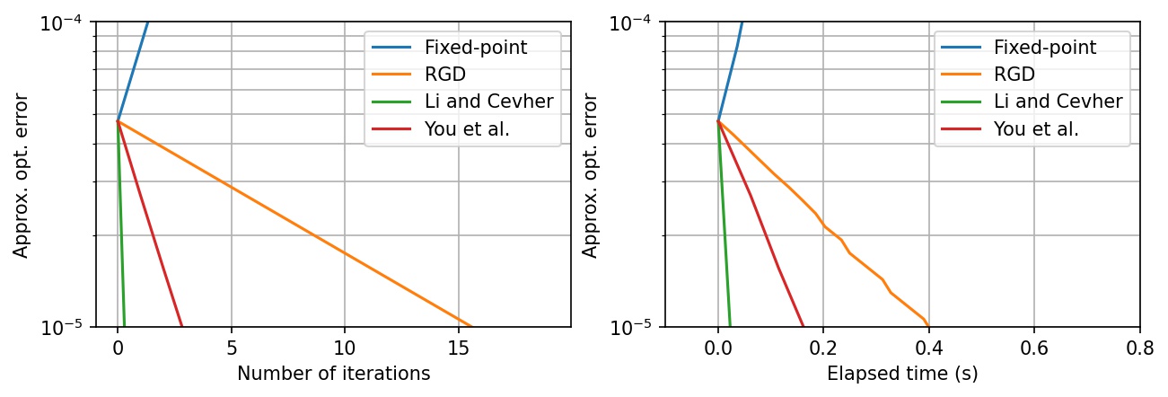
Figure 1: Convergence speeds for computing the order-$3$ Augustin information.

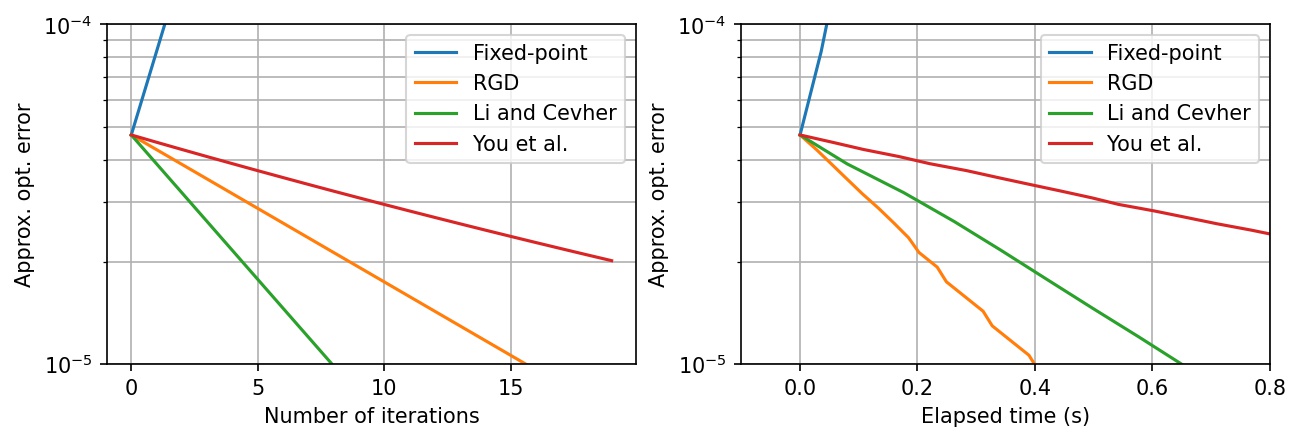
Figure 2: Slower convergence speeds for the methods proposed by Li and Cevher [28] and by You et al. [48].

Figure 1 demonstrates the results of computing the order-$3$ Augustin information using RGD, the fixed-point iteration in Nakıboğlu’s paper [32], the method proposed by Li and Cevher [28], and the method proposed by You et al. [48]. We tuned the parameters for the latter two methods to achieve faster convergence speeds. We set $\bar{\alpha}=0.4$, $r=0.7$, $\tau=0.5$ for the method proposed by Li and Cevher [28], and set $\delta_{1}=1$, $\delta=10^{-5}$, $\beta=0.99$, $\gamma=1.25$, $c=10$ for the method proposed by You et al. [48]. We approximate the optimal value based on the result obtained from the method proposed by Li and Cevher [28] after $20$ iterations.

The numerical results validate our theoretical analysis, showing that RGD converges to the optimum. The fixed-point iteration proposed by Nakiboğlu [32] diverges, as it is only guaranteed to converge for $\alpha<1$. We observe that RGD is slower than the methods proposed by Li and Cevher [28] and by You et al. [48]. However, the latter two methods guarantee only asymptotic convergence, and tuning parameters is required to achieve faster convergence. We found that slightly adjusting parameters can result in slow convergence speed for these two algorithms. Figure 2 shows that if we change $\bar{\alpha}$ from $0.4$ to $0.04$ and $c$ from $10$ to $100$, both methods become slower than RGD in terms of elapsed time. Directly comparing numerical results would be unfair, given that these two methods lack convergence rate guarantees and require tuning to get better results.

6 Conclusion

We have presented an algorithm for computing the order-$\alpha$ Augustin information with a non-asymptotic optimization error guarantee. We have shown that the objective function of the corresponding optimization problem is geodesically $|1-\alpha|$-smooth with respect to the Poincaré metric. With this observation, we propose a hybrid geodesic optimization framework for this optimization problem, and demonstrate that Riemannian gradient descent converges at a rate of $\mathcal{O}(1/T)$ under the hybrid framework.

A potential future direction could be generalizing this result for computing quantum Rényi divergences. Our framework can also be applied to other problems. For instance, the objective functions in the Kelly criterion in mathematical finance [25] and in computing the John Ellipsoid [16] are both g-smooth with respect to the Poincaré metric. Another interesting direction is to develop accelerated or stochastic gradient descent-like algorithms in this hybrid scenario.

Appendices

Appendix A Proof of Lemma 4.5

Since $x_{\infty}\in\mathcal{M}$, by Lemma 4.3, we have

$$\|\mathrm{grad}_{\mathfrak{h}}f(x_{\infty})\|_{\mathfrak{h}(x_{\infty})}=0.$$

Note that $\mathrm{grad}_{\mathfrak{h}}f(x)$ is the (Riesz) representation of the differential form $\mathrm{d}f(x)$ on the tangent space $T_{x}\mathcal{M}$ with respect to the metric $\mathfrak{h}$, and $\mathrm{grad}_{\mathfrak{g}}f(x)$ is the representation of the same differential form $\mathrm{d}f(x)$ under another metric $\mathfrak{g}$. Therefore, for every $v\in T_{x}\mathcal{M}$, we have

$$\langle\mathrm{grad}_{\mathfrak{h}}f(x),v\rangle_{\mathfrak{h}(x)}=\mathrm{d}f(x)[v]=\langle\mathrm{grad}_{\mathfrak{g}}f(x),v\rangle_{\mathfrak{g}(x)},$$

which implies

$$\|\mathrm{grad}_{\mathfrak{g}}f(x_{\infty})\|_{\mathfrak{g}(x_{\infty})}=0.$$

Since $f$ is g-convex with respect to $\mathfrak{g}$, having zero Riemannian gradient with respect to $\mathfrak{g}$ at $x$ is equivalent to $x$ being a global minimizer of $f$ on $\mathcal{M}$.

Appendix B Proof of Theorem 4.6

We have shown that

$$\delta_{t+1}-\delta_{t}\leq-\frac{1}{2L}\frac{\delta_{t}^{2}}{\|(\log_{\mathfrak{g}})_{x_{t}}x_{\infty}\|^{2}_{\mathfrak{h}(x_{t})}}.$$

Let $w_{t}:=\frac{1}{\|(\log_{\mathfrak{g}})_{x_{t}}x_{\infty}\|^{2}_{\mathfrak{h}(x_{t})}}$ and divide both sides by $\delta_{t}\delta_{t+1}$. Since the sequence $\{\delta_{t}\}$ is non-increasing, we write

$$\frac{1}{\delta_{t}}-\frac{1}{\delta_{t+1}}\leq-\frac{w_{t}}{2L}\frac{\delta_{t}}{\delta_{t+1}}\leq-\frac{w_{t}}{2L}.$$

By a telescopic sum, we get

$$-\frac{1}{\delta_{t+1}}\leq\frac{1}{\delta_{1}}-\frac{1}{\delta_{t+1}}\leq-\frac{\sum_{t}w_{t}}{2L}.$$

Therefore, we have

$$f(x_{T+1})-f(x_{\infty})\leq\frac{2L}{\sum w_{t}}\leq\frac{2L}{T}\sup_{t\in\mathbb{N}}\|(\log_{\mathfrak{g}})_{x_{t}}x_{\infty}\|^{2}_{\mathfrak{h}(x_{t})}.$$

Appendix C Proof of Lemma 5.2

Given any vector $x\in\mathbb{R}^{N}_{+}$, we can write it as $x=\lambda y$ where $\lambda=\sum_{i\in[N]}x^{(i)}$ and $y\in\Delta^{N}_{+}$. We have

$$g_{\alpha}(x)=g_{\alpha}(\lambda y)=\lambda-\log\lambda+f_{\alpha}(y).$$

Observe that

$$\frac{\partial}{\partial\lambda}g_{\alpha}=1-\frac{1}{\lambda}$$

and $g_{a}(\lambda y)$ is convex in $\lambda$. This means for every $y\in\Delta^{N}_{+}$, the function $g_{\alpha}(\lambda y)$ achieves its minimum at $\lambda=1$. Therefore, let $y^{\star}$ be a minimizer of $f_{\alpha}$ on $\Delta^{N}_{+}$, for every $\lambda>0$ and $y\in\Delta^{N}_{+}$, we have

$$f_{\alpha}(y^{\star}) \leq f_{\alpha}(y)$$

$$\Leftrightarrow 1+f_{\alpha}(y^{\star}) \leq 1+f_{\alpha}(y)$$

$$\Leftrightarrow g_{\alpha}(y^{\star}) \leq g_{\alpha}(y)\leq g_{\alpha}(\lambda y).$$

This shows that $y^{\star}$ is a minimizer of $f_{\alpha}(y)$ on $\Delta^{N}_{+}$ if and only if $x^{\star}=y^{\star}$ is a minimizer of $g_{\alpha}(x)$.

Appendix D Proof of Lemma 5.3

We will utilize the following equivalent definition of g-convexity and g-smoothness.

Definition D.1 ([49, 21]).

For a function $f:\mathcal{M}\to\mathbb{R}$ defined on $(\mathcal{M},\mathfrak{g})$, we say that $f$ is g-convex on ($\mathcal{M},\mathfrak{g}$) if for every geodesic $\gamma(t):[0,1]\to\mathcal{M}$ connecting any two points $x,y\in\mathcal{M}$, $f(\gamma(t))$ is convex in $t$ in the Euclidean sense. We say that $f$ is g-$L$-smooth ($\mathcal{M},\mathfrak{g}$) if for every geodesic $\gamma(t):[0,1]\to\mathcal{M}$ connecting any two points $x,y\in\mathcal{M}$, $f(\gamma(t))$ is $Ld^{2}(x,y)$-smooth in $t$ in the Euclidean sense.

Let $\gamma(t)$ be the geodesic connecting $x$ and $y$ for $x,y\in\mathbb{R}^{N}_{++}$. If $f_{p}(\gamma(t))$ is $Ld(x,y)$-smooth in the Euclidean sense, then the function $f_{\alpha}(\gamma(t))=\mathbb{E}_{p}f_{p}(\gamma(t))$ is also $Ld(x,y)$-smooth in the Euclidean sense. Therefore, it suffices to prove the g-smoothness for the function $f_{p}(x):=-\frac{1}{1-\alpha}\log\langle p^{\alpha},x^{1-\alpha}\rangle$ for any $p\in\mathbb{R}^{N}_{+}$.

We now prove that

$$f_{p}(\gamma(t))=-\frac{1}{1-\alpha}\log\langle p^{\alpha},\gamma(t)^{1-\alpha}\rangle$$

is $|1-\alpha|d^{2}(x,y)$-smooth in the Euclidean sense. Note that

$$\gamma^{\prime}(t)=\gamma(t)\odot\log(y\oslash x).$$

We have

$$\frac{\mathrm{d}}{\mathrm{d}t}f_{p}(\gamma(t))=-\frac{\langle p^{\alpha},\gamma(t)^{1-\alpha}\odot\log(y\oslash x)\rangle}{\langle p^{\alpha},\gamma(t)^{1-\alpha}\rangle}.$$

The second-order derivative is

$$\frac{\mathrm{d}^{2}}{{\mathrm{d}t}^{2}}f_{p}(\gamma(t)) =(1-\alpha)\bigg{[}\underbrace{\left(\frac{\langle p^{\alpha}\odot\gamma(t)^{1-\alpha},\log(y\oslash x)\rangle}{\langle p^{\alpha},\gamma(t)^{1-\alpha}\rangle}\right)^{2}}_{\text{(1)}}$$

$$-\underbrace{\frac{\langle p^{\alpha}\odot\gamma(t)^{1-\alpha},(\log(y\oslash x))^{2}\rangle}{\langle p^{\alpha},\gamma(t)^{1-\alpha}\rangle}}_{\text{(2)}}\bigg{]}.$$

Note that $p,(\log(y\oslash x))^{2}\in\mathbb{R}^{N}_{+}$ and $\gamma(t)\in\mathbb{R}^{N}_{++}$, so the quantities (1) and (2) are both non-negative. Our strategy is to show that both quantities (1) and (2) are upper bounded by $d^{2}(x,y)$, which then implies

$$\frac{\mathrm{d}^{2}}{{\mathrm{d}t}^{2}}f_{p}(\gamma(t))\in[-|1-\alpha|d^{2}(x,y),|1-\alpha|d^{2}(x,y)].$$

This gives the desired result by the fact that a function is $L$-smooth if and only if its Hessian is upper bounded by $LI$, where $I$ denotes the identity matrix.

D.1 Upper Bound of the quantity (1)

The numerator of the quantity (1) is

$$\langle p^{\alpha}\odot\gamma(t)^{1-\alpha} ,\log(y\oslash x)\rangle^{2}$$

$$\leq\left\|p^{\alpha}\odot\gamma(t)^{1-\alpha}\right\|^{2}_{2}\cdot\left\|\log(y\oslash x))\right\|^{2}_{2}$$

$$\leq\langle p^{\alpha},\gamma(t)^{1-\alpha}\rangle^{2}\left\|\log(y\oslash x))\right\|^{2}_{2}$$

$$=\langle p^{\alpha},\gamma(t)^{1-\alpha}\rangle^{2}d^{2}(x,y).$$

The first inequality is due to the Cauchy-Schwarz inequality, and the second inequality holds because $\sum(x^{(i)})^{2}\leq(\sum x^{(i)})^{2}$ when $x^{(i)}\geq 0$ for all $i\in[N]$. Thus, the quantity (1) is upper bounded by $d^{2}(x,y)$.

D.2 Upper Bound of the quantity (2)

The numerator of the quantity (2) is

$$\langle p^{\alpha}\odot\gamma(t)^{1-\alpha} ,(\log(y\oslash x))^{2}\rangle$$

$$\leq\left\|p^{\alpha}\odot\gamma(t)^{1-\alpha}\right\|_{2}\cdot\left\|(\log(y\oslash x))^{2}\right\|_{2}$$

$$\leq\langle p^{\alpha},\gamma(t)^{1-\alpha}\rangle\left\|\log(y\oslash x))\right\|_{2}^{2}$$

$$=\langle p^{\alpha},\gamma(t)^{1-\alpha}\rangle d^{2}(x,y).$$

The first inequality is due to the Cauchy-Schwarz inequality, and the second inequality is because $\sum(x^{(i)})^{2}\leq(\sum x^{(i)})^{2}$ when $x^{(i)}\geq 0$ for all $i\in[N]$. Thus, the quantity (2) is upper bounded by $d^{2}(x,y)$.

D.3 Geodesic Smoothness of $g_{\alpha}$

We only need to show that $h(x):x\mapsto\langle\mathbbm{1},x\rangle$ is g-1-smooth. By direct calculation, we have

$$\frac{\mathrm{d}^{2}}{{\mathrm{d}t}^{2}}h(\gamma(t)) =\sum(\gamma(t))^{(i)}\left(\log\frac{x^{(i)}}{y^{(i)}}\right)^{2}$$

$$\leq\sum\left(\log\frac{x^{(i)}}{y^{(i)}}\right)^{2}=d^{2}(x,y),$$

where the inequality is due to the concavity and monotonicity of $\log$, which implies

$$(\gamma(t))^{(i)}=(x^{(i)})^{1-t}(y^{(i)})^{t}\leq(1-t)x^{(i)}+ty^{(i)}\leq 1.$$

Appendix E Proof of Lemma 5.4

Let $x\leq\mathbbm{1}$, then the next iterate is

$$x_{+}=x\odot\exp\left(-\frac{1}{|1-\alpha|+1}x\odot\nabla g_{\alpha}(x)\right).$$

A direct calculation shows that $x\odot-\nabla f_{\alpha}(x)\in\Delta^{N}_{+}$, so

$$-x^{(i)}\odot\nabla^{(i)}f_{\alpha}(x)\leq 1,$$

where $\nabla^{(i)}f(x)$ is the $i$-th component of $\nabla f(x)$. By the inequality $\log(a)\leq b(a^{1/b}-1)$ for any $a,b>0$, we have

$$\log x^{(i)} \leq\frac{1}{|1-\alpha|+1}\left((x^{(i)})^{|1-\alpha|+1}-1\right)$$

$$\leq\frac{1}{|1-\alpha|+1}(x^{(i)}-1)$$

$$\leq\frac{1}{|1-\alpha|+1}\left(x^{(i)}+x^{(i)}\nabla^{(i)}f_{\alpha}(x)\right)$$

$$=\frac{1}{|1-\alpha|+1}\left(x^{(i)}\nabla^{(i)}g_{\alpha}(x)\right).$$

Therefore,

$$x^{(i)}\leq\exp\left(\frac{1}{|1-\alpha|+1}\left(x^{(i)}\nabla^{(i)}g_{\alpha}(x)\right)\right).$$

Hence,

$$x^{(i)}_{+}=x^{(i)}\exp\left(-\frac{1}{|1-\alpha|+1}\left(x^{(i)}\nabla^{(i)}g_{\alpha}(x)\right)\right)\leq 1.$$

This gives the desired result.

Appendix F Proof of Lemma 5.5

If the limit $x_{\infty}$ lies in $\mathbb{R}^{N}_{++}$, then it is a minimizer of $f(x)$ by Theorem 4.6. Assume that the limit point $x_{\infty}\in\partial\mathbb{R}^{N}_{++}$ and $x_{\infty}\notin\operatorname*{\arg\min}_{x\in\mathbb{R}^{N}_{+}}f(x)$. Then, by the first-order optimality condition, there exists some $x\in\mathbb{R}^{N}_{+}$ such that

$$\langle\nabla f(x_{\infty}),x-x_{\infty}\rangle=\sum_{i\in[N]}\nabla^{(i)}f(x_{\infty})(x^{(i)}-x^{(i)}_{\infty})<0,$$ (5)

where $\nabla^{(i)}f(x)$ is the $i$-th component of the vector $\nabla f(x)$.

By Lemma 4.3, we have

$$\|\mathrm{grad}f(x_{\infty})\|_{x_{\infty}}=\|x_{\infty}\odot\nabla f(x_{\infty})\|_{2}=0,$$

where the Riemannian gradient is with respect to the Poincaré metric. Therefore,

$$x^{(i)}_{\infty}\neq 0\Rightarrow\nabla^{(i)}f(x_{\infty})=0.$$

Combining this and the inequality (5), we get

$$\sum_{i\in[N],x^{(i)}_{\infty}=0}\nabla^{(i)}f(x_{\infty})x^{(i)}<0,$$

which means there exists some $j\in[N]$ such that

$$\nabla^{(j)}f(x_{\infty})<0\text{ and }x^{(j)}_{\infty}=0.$$

By the continuity of $\nabla f(x)$, there exists an open neighborhood $U\subset\mathbb{R}^{N}$ of $x_{\infty}$ such that for all $x\in U$

$$\nabla^{(j)}f(x)<0.$$

Since $x_{\infty}$ is the limit point of the sequence $\{x_{t}\}$, there exists $T>0$ such that $x_{t}\in U$ for all $t>T$, that is,

$$\nabla^{(j)}f(x_{t})<0.$$

However, this implies

$$-\frac{1}{L}x_{t}^{(j)}\nabla^{(j)}f(x_{t})>0\quad\forall t>T,$$

since $x_{t}\in\mathbb{R}^{N}_{++}$ and $\nabla^{(j)}f(x_{t})<0$. Therefore, by the iteration rule of RGD, we have

$$x_{t+1}^{(j)}=x_{t}^{(j)}\exp\left(-\frac{1}{L}x_{t}^{(j)}\nabla^{(j)}f(x_{t})\right)>x_{t}^{(j)}.$$

This shows that $\{x_{t}^{(j)}\}$ is increasing after $t>T$, which means this sequence cannot converge to $0$. This contradicts our assumption.

Appendix G Proof of Lemma 5.6

Since $g_{\alpha}$ is convex and g-smooth with respect to the Poincaré metric, by Theorem 4.6 and Lemma 5.5, we have

$$g_{\alpha}(x_{T+1})-g_{\alpha}(x^{\star})\leq\frac{2(|1-\alpha|+1)}{T}\sup_{t\in\mathbb{N}}\|x^{\star}\oslash x_{t}-\mathbbm{1}\|_{2}^{2}.$$

Note that for any $\lambda>0$ and a fixed $x\in\Delta^{N}_{+}$, the function $g_{\alpha}(\lambda x)$ is minimized when $\lambda=1$, as shown in Appendix C. Therefore, $x^{\star}\in\Delta^{N}_{+}$, and we have

$$f_{\alpha}(\overline{x}_{T+1})-f_{\alpha}(x^{\star}) =g_{\alpha}(\overline{x}_{T+1})-g_{\alpha}(x^{\star})$$

$$\leq g_{\alpha}(x_{T+1})-g_{\alpha}(x^{\star}).$$

References

• Absil etΒ al. [2008] P-A Absil, Robert Mahony, and Rodolphe Sepulchre. Optimization Algorithms on Matrix Manifolds. Princeton Univ. Press, 2008.
• Antonakopoulos etΒ al. [2020] Kimon Antonakopoulos, ElenaΒ Veronica Belmega, and Panayotis Mertikopoulos. Online and stochastic optimization beyond Lipschitz continuity: A Riemannian approach. In Int. Conf. Learning Representations, 2020.
• Arimoto [1973] S.Β Arimoto. On the converse to the coding theorem for discrete memoryless channels (corresp.). IEEE Trans. Inf. Theory, 19(3):357–359, May 1973. ISSN 0018-9448. doi: 10.1109/TIT.1973.1055007.
• Augustin [1969] U.Β Augustin. Error estimates for low rate codes. Zeitschrift fΓΌr Wahrscheinlichkeitstheorie und Verwandte Gebiete, 14(1):61–88, March 1969. ISSN 0178-8051. doi: 10.1007/BF00534118.
• Augustin [1978] Udo Augustin. Noisy channels. Habilitation Thesis, UniversitΓ€t Erlangen-NΓΌrnberg, 1978.
• Bhatia etΒ al. [2019] Rajendra Bhatia, Tanvi Jain, and Yongdo Lim. On the Bures–Wasserstein distance between positive definite matrices. Expo. Math., 37(2):165–191, 2019.
• Blahut [1974] Richard Blahut. Hypothesis testing and information theory. IEEE Trans. Inf. Theory, 20(4):405–417, July 1974.
• Boumal [2023] Nicolas Boumal. An Introduction to Optimization on Smooth Manifolds. Cambridge Univ. Press, 2023.
• Bubeck etΒ al. [2015] SΓ©bastien Bubeck etΒ al. Convex optimization: Algorithms and complexity. Found. Trends Mach. Learn., 8(3-4):231–357, November 2015.
• Chen etΒ al. [2017] Jun Chen, Da-ke He, Ashish Jagmohan, and LuisΒ A Lastras-MontaΓ±o. On the reliability function of variable-rate Slepian-Wolf coding. Entropy, 19(8):389, July 2017.
• Cheng and Nakiboğlu [2021] Hao-Chung Cheng and Barış Nakiboğlu. On the existence of the Augustin mean. In 2021 IEEE Information Theory Workshop (ITW), pages 1–6, 2021.
• Cheng etΒ al. [2019] Hao-Chung Cheng, Min-Hsiu Hsieh, and Marco Tomamichel. Quantum sphere-packing bounds with polynomial prefactors. IEEE Trans. Inf. Theory, 65(5):2872–2898, January 2019. doi: 10.1109/tit.2019.2891347.
• Cheng etΒ al. [2022a] Hao-Chung Cheng, LiΒ Gao, and Min-Hsiu Hsieh. Properties of noncommutative rΓ©nyi and Augustin information. Commun. Math. Phys., 390(2):501–544, March 2022a.
• Cheng etΒ al. [2022b] Hao-Chung Cheng, EricΒ P Hanson, Nilanjana Datta, and Min-Hsiu Hsieh. Duality between source coding with quantum side information and classical-quantum channel coding. IEEE Trans. Inf. Theory, 68(11):7315–7345, June 2022b.
• Chewi etΒ al. [2020] Sinho Chewi, Tyler Maunu, Philippe Rigollet, and AustinΒ J Stromme. Gradient descent algorithms for Bures-Wasserstein barycenters. In Conf. Learning Theory, pages 1276–1304, 2020.
• Cohen etΒ al. [2019] MichaelΒ B Cohen, Ben Cousins, YinΒ Tat Lee, and Xin Yang. A near-optimal algorithm for approximating the John Ellipsoid. In Conf. Learning Theory, pages 849–873, 2019.
• CsiszΓ‘r [1995] Imre CsiszΓ‘r. Generalized cutoff rates and RΓ©nyi’s information measures. IEEE Trans. Inf. Theory, 41(1):26–34, January 1995. doi: 10.1109/18.370121.
• CsiszΓ‘r and KΓΆrner [2011] Imre CsiszΓ‘r and JΓ‘nos KΓΆrner. Information Theory: Coding Theorems for Discrete Memoryless Systems. Cambridge Univ. Press, 2011.
• Dalai and Winter [2017] Marco Dalai and Andreas Winter. Constant compositions in the sphere packing bound for classical-quantum channels. IEEE Trans. Inf. Theory, 63(9):5603–5617, July 2017.
• Dueck and Korner [1979] G.Β Dueck and J.Β Korner. Reliability function of a discrete memoryless channel at rates above capacity (corresp.). IEEE Trans. Inf. Theory, 25(1):82–85, January 1979. ISSN 0018-9448. doi: 10.1109/TIT.1979.1056003.
• Han etΒ al. [2021] Andi Han, Bamdev Mishra, PratikΒ Kumar Jawanpuria, and Junbin Gao. On Riemannian optimization over positive definite matrices with the Bures-Wasserstein geometry. Adv. Neural Information Processing Systems, 34:8940–8953, December 2021.
• Haroutunian [1968] EAΒ Haroutunian. Bounds for the exponent of the probability of error for a semicontinuous memoryless channel. Problemy Peredachi Informatsii, 4(4):37–48, 1968.
• Hosseini and Sra [2015] Reshad Hosseini and Suvrit Sra. Matrix manifold optimization for Gaussian mixtures. Adv. Neural Information Processing Systems, 28, 2015.
• Hosseini and Sra [2020] Reshad Hosseini and Suvrit Sra. An alternative to EM for Gaussian mixture models: batch and stochastic Riemannian optimization. Math. Program., 181(1):187–223, May 2020.
• Kelly [1956] JohnΒ L Kelly. A new interpretation of information rate. Bell Syst. Tech. J., 35(4):917–926, July 1956.
• Lan [2020] Guanghui Lan. First-order and Stochastic Optimization Methods for Machine Learning. Springer, 2020.
• Lee [2018] JohnΒ M Lee. Introduction to Riemannian Manifolds. Springer, 2018.
• Li and Cevher [2019] Yen-Huan Li and Volkan Cevher. Convergence of the exponentiated gradient method with Armijo line search. J. Optim. Theory Appl., 181(2):588–607, May 2019.
• Mojahedian etΒ al. [2019] MohammadΒ Mahdi Mojahedian, Salman Beigi, Amin Gohari, MohammadΒ Hossein Yassaee, and MohammadΒ Reza Aref. A correlation measure based on vector-valued $L_{p}$-norms. IEEE Trans. Inf. Theory, 65(12):7985–8004, August 2019.
• Mosonyi and Ogawa [2017] M.Β Mosonyi and T.Β Ogawa. Strong converse exponent for classical-quantum channel coding. Commun. Math. Phys., 355(1):373–426, October 2017. ISSN 1432-0916. doi: 10.1007/s00220-017-2928-4.
• Mosonyi and Ogawa [2021] M.Β Mosonyi and T.Β Ogawa. Divergence radii and the strong converse exponent of classical-quantum channel coding with constant compositions. IEEE Trans. Inf. Theory, 67(3):1668–1698, December 2021.
• Nakiboğlu [2019] Barış Nakiboğlu. The Augustin capacity and center. Probl. Inf. Transm., 55:299–342, October 2019.
• Nakiboğlu [2020] BARIŞ Nakiboğlu. A simple derivation of the refined sphere packing bound under certain symmetry hypotheses. Turkish J. Math., 44(3):919–948, 2020.
• Nesterov etΒ al. [2018] Yurii Nesterov etΒ al. Lectures on Convex Optimization. Springer, 2018.
• Omura [1975] J.Β K. Omura. A lower bounding method for channel and source coding probabilities. Inf. Control., 27(2):148–177, February 1975. ISSN 0019-9958. doi: 10.1016/S0019-9958(75)90120-5.
• Pennec [2020] Xavier Pennec. Manifold-valued image processing with SPD matrices. In Riemannian Geometric Statistics in Medical Image Analysis, pages 75–134. Elsevier, 2020.
• Pennec etΒ al. [2006] Xavier Pennec, Pierre Fillard, and Nicholas Ayache. A Riemannian framework for tensor computing. Int. J. Comput. Vis., 66:41–66, January 2006.
• Rapcsak [1991] Tamas Rapcsak. Geodesic convexity in nonlinear optimization. J. Optim. Theory Appl., 69(1):169–183, April 1991.
• RΓ©nyi [1961] AlfrΓ©d RΓ©nyi. On measures of entropy and information. In Proc. 4th Berkeley Symp. Mathematical Statistics and Probability, Volume 1: Contributions to the Theory of Statistics, volumeΒ 4, pages 547–562, 1961.
• Shen etΒ al. [2023] Yu-Chen Shen, LiΒ Gao, and Hao-Chung Cheng. Privacy amplification against quantum side information via regular random binning. In 2023 59th Annu. Allerton Conference on Communication, Control, and Computing (Allerton), pages 1–8, 2023.
• Udriste [1994] Constantin Udriste. Convex functions and optimization methods on Riemannian manifolds. Springer Science & Business Media, 1994.
• van Erven and Harremoes [2014] Tim van Erven and Peter Harremoes. RΓ©nyi divergence and Kullback-Leibler divergence. IEEE Trans. Inf. Theory, 60(7):3797–3820, June 2014. doi: 10.1109/tit.2014.2320500.
• Verdu [2015] Sergio Verdu. $\alpha$-mutual information. In 2015 Information Theory and Applications Workshop (ITA), pages 1–6, 2015.
• VerdΓΊ [2021] Sergio VerdΓΊ. Error exponents and $\alpha$-mutual information. Entropy, 23(2):199, August 2021.
• Vishnoi [2018] NisheethΒ K Vishnoi. Geodesic convex optimization: Differentiation on manifolds, geodesics, and convexity. 2018. arXiv:1806.06373.
• Weber and Sra [2023] Melanie Weber and Suvrit Sra. Global optimality for Euclidean CCCP under Riemannian convexity. In Int. Conf. Machine Learning, pages 36790–36803, 2023.
• Wiesel [2012] Ami Wiesel. Geodesic convexity and covariance estimation. IEEE Trans. Signal Process., 60(12):6182–6189, September 2012.
• You etΒ al. [2022] Jun-Kai You, Hao-Chung Cheng, and Yen-Huan Li. Minimizing quantum RΓ©nyi divergences via mirror descent with Polyak step size. In 2022 IEEE Int. Symp. Information Theory (ISIT), pages 252–257, 2022.
• Zhang and Sra [2016] Hongyi Zhang and Suvrit Sra. First-order methods for geodesically convex optimization. In Conf. Learning Theory, pages 1617–1638, 2016.
• Zhang etΒ al. [2013] Teng Zhang, Ami Wiesel, and MariaΒ Sabrina Greco. Multivariate generalized Gaussian distribution: Convexity and graphical models. IEEE Trans. Signal Process., 61(16):4141–4148, June 2013.