A Local Projection Stabilised HHO Method for the Oseen Problem

Abstract

Fluid flow problems with high Reynolds number show spurious oscillations in their solution when solved using standard Galerkin finite element methods. These Oscillations can be eradicated using various stabilisation techniques. In this article, we use a local projection stabilisation for a Hybrid High-Order approximation of the Oseen problem. We prove an existence-uniqueness result under a SUPG-like norm. We derive an optimal order error estimate under this norm for equal order polynomial discretisation of velocity and pressure spaces.

Introduction

The Navier-Stokes equation models the flow of fluid in a domain. A solution to these equations is important in many engineering problems. Linearizing and time-discretizing the Navier-Stokes equation, we obtain the Oseen problem:

$$-\epsilon\Delta\boldsymbol{u}+(\boldsymbol{b}\cdot\nabla)\boldsymbol{u}+\sigma\boldsymbol{u}+\nabla p= \boldsymbol{f}\text{ in }\Omega,$$ (0.1)

$${\rm div~{}}\boldsymbol{u}= 0\text{ in }\Omega$$

$$\boldsymbol{u}= 0\text{ on }\partial\Omega,$$

where $\boldsymbol{u}$ denotes the velocity of the fluid and $p$ denotes the pressure. Here $\Omega\subset\mathbb{R}^{2}$ is a polygonal domain with boundary $\partial\Omega$. The force function $\boldsymbol{f}$ is in $[L^{2}(\Omega)]^{2}$. The viscosity coefficient is denoted by $\epsilon$, where $0<\epsilon\ll 1$. The convection coefficient $\boldsymbol{b}$ is a $[W^{1}_{\infty}(\Omega)]^{2}$ function such that ${\rm div~{}}\boldsymbol{b}=0$. The reaction coefficient is a positive constant denoted by $\sigma$ with $\sigma\leq\sigma_{0}$.

Fluid flow problems with dominant convection produce boundary and interior layers. It is well-known that the numerical solution to these problems using the usual Galerkin method cannot capture these small layers. Instead, they produce nonphysical solutions which contain spurious oscillations. To eliminate the effect of convection, one can add stabilisations. In this article, we focus on local projection stabilisation using a Hybrid High-Order approximation on general polygonal meshes.

In the last few years, there has been a growing interest in high-order polynomial approximations of solutions to PDEs on general polytopal meshes. Due to the vast literature in this area, we cite a few well-known works: the Hybridizable Discontinuous Galerkin (HDG) method in [24, 28]. The HDG has been further extended to the convection diffusion problem in [23] and the Oseen problem in [19]. The Virtual Element method (VEM) has been studied in [5, 6, 13]. The VEM has also been applied to the convection diffusion problem with SUPG stabilisation [7] and to the Oseen problem with LPS stabilisation [50]. The Weak Galerkin method is introduced in [51, 54, 55] and the Gradient Discretisation method is introduced in [40, 37, 27]. The Multiscale Hybrid-Mixed method has been studied in [2]. The focus of our article is on the Hybrid High-Order (HHO) method, originally introduced in [30, 29]. For an overview of the HHO method, we refer to [25]. HHO is a robust method based on a local polynomial reconstruction. It is independent of the dimension of the problem and suitable for local static condensation, which drastically reduces the computational cost of the matrix solver.

The HHO method is closely related to the HDG method but they differ in the choice of stabilisation, see [22] for details. In the nonconforming Virtual Element methods (ncVEM) one takes the projection of the virtual function in the stabilisation, whereas the HHO method takes a reconstruction of the function in the stabilisation. In [49], the connection of the HHO method with the virtual element method is discussed. See [9, 38, 14, 15, 48] for related works. In the lowest-order case ($k=0$), the HHO method resembles the Hybrid Mixed Mimetic family, hence the mixed-hybrid Mimetic Finite Differences, the Hybrid Finite Volume and the Mixed Finite Volume methods too, see [39, 16, 42, 35, 36]. We state the following predominant works on the HHO methods: problem with pure diffusion [30], advection-diffusion problem [26], interface problems [18], for linear PDEs, elliptic obstacle problem [21], Stokes problem [31], the Oseen problem [1] and the steady incompressible Navier Stokes equations [32].

In the study of stabilisations for fluid flow problems with high Reynolds number, the SUPG method by Hughes and Brooks [17] is the most well-known. SUPG is studied for the incompressible Navier Stokes equation in [53]. There is a wide range of stabilisation techniques in the literature, some of them are: the method of least squares [52], residual free bubbles technique [52], continuous interior penalty method [52] and the discontinuous Galerkin method [52]. In this article, we are interested in the local projection stabilisation scheme, originally introduced for the Stokes problem by Becker and Braack [3] for the Stokes problem. It has also been studied for the transport problem, scalar convection diffusion problem, the Oseen problem and the Navier stokes equations [4, 52, 11, 10, 12]. A non-conforming patchwise LPS scheme using Crouzeix-Raviart elements for the convection diffusion problem has been studied in [34] and for the Oseen problem in [8]. A generalised version of LPS has been studied by Knobloch for the convection diffusion problem [46] and also for the Oseen problem [47].

The SUPG method naturally gives an additional control on the advective derivative of velocity; however, the usual LPS schemes in [4, 10] do not provide this. Moreover, the LPS schemes in [4, 10] work through a two-level mesh approach or through enrichment. The articles [4, 10, 46, 47] need to satisfy a local inf-sup condition necessary for error analysis and stability. In this article, we employ a generalised LPS technique to design an HHO scheme for the Oseen problem motivated by the work in [1] on the HHO approximation for the Oseen problem. The additional LPS term provides control on the advective derivative. Moreover, we employ a one-level approach that does not require any enrichment of the discrete spaces and the need for a local inf-sup condition as seen in [47].

In this article, along with the LP stabilisation, we have added another velocity stabilisation to control the normal jump of the solution. This helps to further stabilize the solution. Moreover, we also need pressure stabilisation to stabilise the gradient of pressure. In a nutshell, the LPS-HHO scheme is a combination of a usual HHO method for the Oseen problem combined with the above stabilisations along with an upwind term. Comparing this article with [1], we have proven that the LPS stabilisation term in the formulation helps to prove a stability result under a stronger SUPG-like norm. Moreover, in this article, the presence of normal jump stabilisation in the discrete scheme gives epsilon robust error bounds. This can be seen in the inequality (4).

The rest of the article is organised as follows: Section 1 defines the Oseen problem along with some notation and preliminaries. Section 2 deals with discrete HHO formulation of the Oseen equations. Section 3 provides the proof for the discrete well-posedness of the system in Section 2. Section 5 provides the a priori error estimates. Numerical results are provided in Section 6. From now on, we denote by $a\lesssim b$ the expression $a\leq Cb$, where $C$ is a positive constant. The analysis is done on standard $k$th order Sobolev spaces $H^{k}(\Omega)$. Sobolev spaces with zero trace is denoted by $H^{k}_{0}(\Omega)$ with the standard norm $\left\|\cdot\right\|_{k}=\sum_{|\alpha|\leq k}\left\|D^{\alpha}\cdot\right\|_{L^{2}(\Omega)}$. $L^{2}_{0}(\Omega)$ represents the space of square integrable functions with zero mean. For $M\subset\Omega,k\geq 0$ and $1\leq p\leq\infty$, let $\|.\|_{k,p,M}$ be the norm on the $k-$th order Sobolev space $W^{k,p}(M)$. For $p=2$ we denote the norm by $\|.\|_{k,M}$.

1 Continuous Problem, Notations and Preliminaries

In this section, we introduce the weak formulation of the Oseen problem (0.1) and some preliminaries. Let $\boldsymbol{V}=[H^{1}_{0}(\Omega)]^{2}$ be the velocity space and $Q=L^{2}_{0}(\Omega)$ be the pressure space. The weak formulation for the Oseen problem (0.1) is given by: Find $\boldsymbol{u}\in\boldsymbol{V}$ and $p\in Q$ such that

$$a(\boldsymbol{u},\boldsymbol{v})-b(p,\boldsymbol{v}) =(\boldsymbol{f},\boldsymbol{v})\quad{\rm for~{}all}~{}\boldsymbol{v}\in\boldsymbol{V},$$ (1.1)

$$b(q,\boldsymbol{u}) =0\quad{\rm for~{}all}~{}q\in Q,$$

where, the bilinear forms $a(\cdot,\cdot)$ and $b(\cdot,\cdot)$ are defined as

$$a(\boldsymbol{u},\boldsymbol{v}) :=\epsilon(\nabla\boldsymbol{u},\nabla\boldsymbol{v})_{L_{2}(\Omega)}+((\boldsymbol{b}\cdot\nabla)\boldsymbol{u},\boldsymbol{v})_{L_{2}(\Omega)}+(\sigma\boldsymbol{u},\boldsymbol{v})_{L_{2}(\Omega)},$$

$$b(q,\boldsymbol{u}) :=(q,{\rm div~{}}\boldsymbol{u})_{L_{2}(\Omega)}.$$

Using the fact that ${\rm div~{}}\boldsymbol{b}=0$ and $\sigma>0$, one can show that the bilinear form $a(\boldsymbol{u},\boldsymbol{v})$ is coercive. It is well known that the bilinear form $b(q,\boldsymbol{u})$ is inf-sup stable for $\boldsymbol{u}\in[H^{1}_{0}(\Omega)]^{2}$ and $q\in L^{2}_{0}(\Omega)$. Therefore, the existence and uniqueness of the problem (1.1) can be shown using the Babuška-Brezzi condition, see [43, Chapter IV]. An equivalent formulation for (1.1) seeks $(\boldsymbol{u},p)\in\boldsymbol{V}\times Q$ such that

$$A((\boldsymbol{u},p),(\boldsymbol{v},q))=(\boldsymbol{f},\boldsymbol{v}),\quad\text{for all}\quad(\boldsymbol{v},q)\in\boldsymbol{V}\times Q,$$ (1.2)

where, the combined bilinear form is defined by

$$A((\boldsymbol{u},p),(\boldsymbol{v},q)):=a(\boldsymbol{u},\boldsymbol{v})-b(p,\boldsymbol{v})+b(q,\boldsymbol{u}).$$

The existence and uniqueness of the problem (1.2) can be proved in a similar manner. Henceforth, we will use this combined mixed formulation in our analysis.

Consider a decomposition $\mathcal{T}_{h}$ of the domain $\Omega$ into a finite collection of nonempty, disjoint, open polygons. Let $h_{T}$ denote the diameter of a polygon $T\in\mathcal{T}_{h}$. The subscript $h$ in $\mathcal{T}_{h}$ denotes the maximum diameter among all polygons $T$, that is $h:=\max_{T\in\mathcal{T}_{h}}h_{T}$. The edges/faces of a polygon $T$ are denoted by $F$. The collection of all faces (skeleton ) of the decomposition $\mathcal{T}_{h}$ is denoted by $\mathcal{F}_{h}$. The set of all interior faces is denoted by $\mathcal{F}_{h}^{i}$ and the set of all boundary faces by $\mathcal{F}_{h}^{b}$. Length of a face $F$ is denoted by $h_{F}$. We assume that the diameter of the polygons in $\mathcal{T}_{h}$ are uniformly comparable to the face lengths, that is, $h_{T}\lesssim h_{F}\lesssim h_{T}$. For a polygon $T$, let the collection of edges of $T$ be denoted by $\mathcal{F}_{T}$. We assume that there exists a constant $N$ such that $\max_{T\in\mathcal{T}_{h}}\#\mathcal{F}_{T}\leq N$. This condition restricts the polygons from having too many faces.

Next, we define the hybrid discrete spaces on the decomposition $\mathcal{T}_{h}$. For any bounded domain $S$, let $P^{k}(S)$ denote the space of polynomials defined on $S$ of degree at most $k\geq 0$. The local degrees of freedom on each polygon $T\in\mathcal{T}_{h}$ is given by

$$\underline{\boldsymbol{U}}_{T}^{k}:=\{\underline{\boldsymbol{v}}_{T}=(\boldsymbol{v}_{T},(\boldsymbol{v}_{F})_{F\in\mathcal{F}_{T}}):\boldsymbol{v}_{T}\in[P^{k}(T)]^{2}\text{ and }\boldsymbol{v}_{F}\in[P^{k}(F)]^{2},F\in\mathcal{F}_{T}\}.$$

The global degrees of freedom is given by combining the face values of $\underline{\boldsymbol{U}}_{T}^{k}$ as

$$\underline{\boldsymbol{U}}_{h}^{k}:=\{\underline{\boldsymbol{v}}_{h}=((\boldsymbol{v}_{T})_{T\in\mathcal{T}_{h}},(\boldsymbol{v}_{F})_{F\in\mathcal{F}_{h}})\}.$$

The hybrid space with zero boundary condition is defined as

$$\underline{\boldsymbol{U}}_{h,0}^{k}:=\{\underline{\boldsymbol{v}}_{h}\in\underline{\boldsymbol{U}}_{h}^{k}:\boldsymbol{v}_{F}=0\text{ for all }F\in\mathcal{F}_{h}^{b}\}.$$

The restriction of $\underline{\boldsymbol{v}}_{h}\in\underline{\boldsymbol{U}}_{T}^{k}$ on a polygon $T$ is denoted by $\boldsymbol{v}_{T}$. The local interpolation operator $\underline{\boldsymbol{I}}_{T}^{k}:[H^{1}(T)]^{2}\rightarrow\underline{\boldsymbol{U}}_{T}^{k}$ is given by

$$\underline{\boldsymbol{I}}_{T}^{k}\boldsymbol{v}:=((\pi_{T}^{k}\boldsymbol{v}),(\pi_{F}^{k}\boldsymbol{v}\rvert_{F})_{F\in\mathcal{F}_{T}}),$$

where $\pi_{T}^{k}$ and $\pi_{F}^{k}$ are $L^{2}$ orthogonal projection onto $[P^{k}(T)]^{2}$ and $[P^{k}(F)]^{2}$ respectively. In a similar manner, the global interpolation operator $\underline{\boldsymbol{I}}_{h}^{k}\boldsymbol{v}:[H^{1}(\Omega)]^{2}\rightarrow\underline{\boldsymbol{U}}_{h}^{k}$ is defined as follows

$$\underline{\boldsymbol{I}}_{h}^{k}\boldsymbol{v}:=((\pi_{T}^{k}\boldsymbol{v})_{T\in\mathcal{T}_{h}},(\pi_{F}^{k}\boldsymbol{v})_{F\in\mathcal{F}_{h}}).$$

Note that the projection operators are applied on vectors component-wise. The discrete pressure space is the usual piecewise polynomial space of degree $k$ with zero mean

$$P_{h}^{k}:=\{p_{h}\in L^{2}(\Omega):p_{h}|_{T}\in P^{k}(T)\}\cap L^{2}_{0}(\Omega).$$

We recall some standard inequalities which will be used throughout the article.

Inverse Inequality: There exists a positive constant $C$ independent of the meshsize $h_{T}$ such that for any $v_{h}\in P^{k}(T)$ we have

$$\left\|\nabla\boldsymbol{v}_{h}\right\|_{L^{2}(T)}\leq Ch_{T}^{-1}\left\|\boldsymbol{v}_{h}\right\|_{L^{2}(T)}.$$

Trace Inequality:  [28, pp. 27] There exists a positive constant $C$ independent of the meshsize $h_{T}$ such that

$$\|v\|_{L^{2}(\partial T)}\leq C(h_{T}^{-1/2}\|v\|_{L^{2}(T)}+h_{T}^{1/2}\|\nabla v\|_{L^{2}(T)})\quad\forall v\in H^{1}(T).$$

In particular, for $v_{h}\in P^{k}(T)$ and $F\in\mathcal{F}_{T}$, it holds

$$\|v_{h}\|_{L^{2}(F)}\leq Ch_{T}^{-1/2}\|v_{h}\|_{L^{2}(T)}.$$

Discrete Poincare inequality: There exists a positive constant $C$ independent of $h_{T}$ such that for $\underline{\boldsymbol{v}}_{h}\in\underline{\boldsymbol{U}}_{h,0}^{k}$ we have

$$\left\|\boldsymbol{v}_{h}\right\|\leq C\Big{(}\sum_{T\in\mathcal{T}_{h}}\left\|\nabla\boldsymbol{v}_{T}\right\|_{T}^{2}+\sum_{T\in\mathcal{T}_{h}}\sum_{F\in\mathcal{F}_{T}}\frac{1}{h_{F}}\int_{F}(\boldsymbol{v}_{F}-\boldsymbol{v}_{T})^{2}\Big{)}^{1/2}.$$ (1.3)

Approximation property of $L^{2}$ orthogonal projection:  [28, lemma 1.58] The $L^{2}$-projection $\pi_{T}^{k}$ satisfies the following approximation property: for any $\boldsymbol{v}\in H^{s}(T)$ with $s\in\{1,2,...,k+1\}$

$$\lvert\boldsymbol{v}-\pi_{T}^{k}\boldsymbol{v}\rvert_{H^{m}(T)}+h_{T}^{1/2}\lvert\boldsymbol{v}-\pi_{T}^{k}\boldsymbol{v}\rvert_{H^{m}(\partial T)}\leq Ch_{T}^{s-m}\lvert\boldsymbol{v}\rvert_{H^{s}(T)}\quad m\in\{0,1,...,s-1\}.$$ (1.4)

Let the outward unit normal component for a polygon $T\in\mathcal{T}_{h}$ be denoted by $\boldsymbol{n}_{T}$. Similarly the outward unit normal for a face $F\in\mathcal{F}_{T}$ is given by $\boldsymbol{n}_{TF}$ such that $\boldsymbol{n}_{T}\rvert_{F}=\boldsymbol{n}_{TF}$. Moreover, the normal component of the convection term on a face $F\in\mathcal{F}_{T}$ is defined as $\boldsymbol{b}_{TF}:=\boldsymbol{b}\rvert_{F}\cdot\boldsymbol{n}_{TF}$. The jump of a scalar-valued function $v$ on a face $F$ shared by two polygons $T_{1}$ and $T_{2}$ is given by

$$\left[\hskip-3.5pt\left[v\right]\hskip-3.5pt\right]=v\rvert_{T_{1}}-v\rvert_{T_{2}}.$$

The sign of $\left[\hskip-3.5pt\left[v\right]\hskip-3.5pt\right]$ is adjusted according to the direction of the outward normal. For a vector-valued function $\boldsymbol{v}=(v_{1},v_{2})$

$$\nabla\boldsymbol{v}:=\begin{pmatrix}\frac{\partial v_{1}}{\partial x}&\frac{\partial v_{1}}{\partial y}\\ \frac{\partial v_{2}}{\partial x}&\frac{\partial v_{2}}{\partial y}\end{pmatrix},\hskip 14.22636pt\frac{\partial\boldsymbol{v}}{\partial\boldsymbol{n}}:=\nabla\boldsymbol{v}\cdot\boldsymbol{n}\;\;{\rm and}\;\;(\nabla\boldsymbol{u},\nabla\boldsymbol{v})_{L^{2}(\Omega)}:=\int_{\Omega}\sum_{i,j=1}^{2}(\nabla\boldsymbol{u})_{i,j}(\nabla\boldsymbol{v})_{i,j}{\rm~{}dx}.$$

Let $|v|$ denote the modulus function of $v$. The positive and negative part of $v$ is defined as

$$v^{\oplus}:=\frac{1}{2}(|v|+v)\text{ and }v^{\ominus}:=\frac{1}{2}(|v|-v).$$

2 Discrete Oseen Problem with LPS stabilisation

In this section, we introduce the LPS stabilised discrete formulation for the Oseen problem (1.2) on the hybrid space $\underline{\boldsymbol{U}}_{h,0}^{k}\times P_{h}^{k}$. This section is divided into three sub-sections. The first part defines some reconstruction operators which are essential to define the HHO scheme. In the second part, we discuss a generalised local projection stabilisation setup. The discrete LPS-HHO scheme is defined in the third sub-section.

2.1 Local Reconstructions

We define three reconstruction operators on the local spaces $\underline{\boldsymbol{U}}_{T}^{k}$, see [1]. These will be used to define the discrete HHO bilinear form in (2.7).

Local velocity reconstruction: The velocity reconstruction operator $\boldsymbol{r}_{T}^{k+1}:\underline{\boldsymbol{U}}_{T}^{k}\rightarrow[P^{k+1}(T)]^{2}$ is defined as follows: For any $\underline{\boldsymbol{v}}_{T}\in\underline{\boldsymbol{U}}_{T}^{k}$, $\boldsymbol{r}_{T}^{k+1}\underline{\boldsymbol{v}}_{T}$ must satisfy

$$(\nabla(\boldsymbol{r}_{T}^{k+1}\underline{\boldsymbol{v}}_{T}),\nabla\boldsymbol{w})_{T} =(\nabla\boldsymbol{v}_{T},\nabla\boldsymbol{w})_{T}+\sum_{F\in\mathcal{F}_{T}}(\boldsymbol{v}_{F}-\boldsymbol{v}_{T},\nabla\boldsymbol{w}\cdot\boldsymbol{n}_{TF})_{F}\quad\forall\boldsymbol{w}\in[P^{k+1}(T)]^{2},$$ (2.1)

$$(\boldsymbol{r}_{T}^{k+1}\underline{\boldsymbol{v}}_{T},1)_{T} =(\boldsymbol{v}_{T},1)_{T}.$$

Approximation property of $\boldsymbol{r}_{T}^{k+1}$: There exists a real number $C>0$, depending on $\varrho$ but independent of $h_{T}$ such that, for all $\boldsymbol{v}\in[H^{s+1}(T)]^{2}$ for some $s\in\{0,1,\ldots,k+1\}$,

$$\|\boldsymbol{v}-\boldsymbol{r}_{T}^{k+1}\underline{\boldsymbol{I}}_{T}^{k}\boldsymbol{v}\|_{T}+h_{T}^{1/2}\|\boldsymbol{v}-\boldsymbol{r}_{T}^{k+1}\underline{\boldsymbol{I}}_{T}^{k}\boldsymbol{v}\|_{\partial T}+h_{T}\|\nabla(\boldsymbol{v}-\boldsymbol{r}_{T}^{k+1}\underline{\boldsymbol{I}}_{T}^{k}\boldsymbol{v})\|_{T}\leq Ch_{T}^{s+1}\|\boldsymbol{v}\|_{H^{s+1}(T)}.$$

For $s\in\{1,2,...,k+1\}$ and $\boldsymbol{v}\in[H^{s+1}(T)]^{2}$ we also have the approximation property

$$\|\nabla(\boldsymbol{v}-\boldsymbol{r}_{T}^{k+1}\underline{\boldsymbol{I}}_{T}^{k}\boldsymbol{v})\|_{\partial T}\leq Ch_{T}^{s-1/2}\|\boldsymbol{v}\|_{H^{s+1}(T)}.$$ (2.2)

Local advection reconstruction operator: $\boldsymbol{G}_{\boldsymbol{b},T}^{k}:\underline{\boldsymbol{U}}_{T}^{k}\rightarrow[P^{k}(T)]^{2}$ is defined as follows: For any $\underline{\boldsymbol{v}}_{T}\in\underline{\boldsymbol{U}}_{T}^{k}$

$$(\boldsymbol{G}_{\boldsymbol{b},T}^{k}(\underline{\boldsymbol{v}}_{T}),\boldsymbol{w}_{T})_{T}=(\boldsymbol{b}\cdot\nabla\boldsymbol{v}_{T},\boldsymbol{w}_{T})_{T}+\sum_{F\in\mathcal{F}_{T}}(\boldsymbol{b}_{TF}(\boldsymbol{v}_{F}-\boldsymbol{v}_{T}),\boldsymbol{w}_{T})\quad\forall\boldsymbol{w}_{T}\in[P^{k}(T)]^{2}.$$ (2.3)

Local divergence reconstruction operator: $D_{T}^{k}:\underline{\boldsymbol{U}}_{T}^{k}\rightarrow P^{k}(T)$ is defined as follows: For any $\underline{\boldsymbol{v}}_{T}\in\underline{\boldsymbol{U}}_{T}^{k}$

$$(D_{T}^{k}(\underline{\boldsymbol{v}}_{T}),q)_{T}=({\rm div~{}}\boldsymbol{v}_{T},q)_{T}+\sum_{F\in\mathcal{F}_{T}}((\boldsymbol{v}_{F}-\boldsymbol{v}_{T})\cdot\boldsymbol{n}_{TF},q)_{F}\quad\forall q\in P^{k}(T).$$ (2.4)

2.2 A local Projection Setting

Let $\mathcal{M}_{h}$ be a finite decomposition of the domain $\Omega$ into open polygons, possibly overlapping so that $\cup_{M\in\mathcal{M}_{h}}\bar{M}=\bar{\Omega}$ and each $M\in\mathcal{M}_{h}$ is a collection of $T\in\mathcal{T}_{h}$. We assume that for all $M\in\mathcal{M}_{h}$ there exists a constant $C$ such that for any $M\in\mathcal{M}_{h}$ the cardinality of the set $\{N\in\mathcal{M}_{h}:N\cap M\neq\phi\}\leq C$. Let $h_{M}$ denote the diameter of the cell $M$. We also assume that for any polygon $T\in\mathcal{T}_{h}$ inside $M\in\mathcal{M}_{h}$, $h_{M}\lesssim h_{T}$. Let $K_{M}:[L^{2}(M)]^{2}\rightarrow[P^{k-1}(M)]^{2}$ be a bounded linear operator defined by $K_{M}:=Id_{M}-\pi^{k-1}_{M}$, $Id_{M}$ being the identity map.

Let $\boldsymbol{b}_{M}$ to be a piecewise constant approximation of $\boldsymbol{b}$ on $M$ such that $\left\|\boldsymbol{b}_{M}\right\|_{0,\infty,M}\leq C\left\|\boldsymbol{b}\right\|_{0,\infty,M}$ and $\left\|\boldsymbol{b}-\boldsymbol{b}_{M}\right\|_{0,\infty,M}\leq Ch_{M}\lvert\boldsymbol{b}\rvert_{1,\infty,M}$. For each cell $T$ contained in $M$, we define a local reconstruction $\boldsymbol{G}_{\boldsymbol{b}_{M},T}:\underline{\boldsymbol{U}}_{T}^{k}\rightarrow[P^{k}(T)]^{2}$ as follows: For $\underline{\boldsymbol{v}}_{T}\in\underline{\boldsymbol{U}}_{T}^{k}$

$$(\boldsymbol{G}_{\boldsymbol{b}_{M},T}^{k}(\underline{\boldsymbol{v}}_{T}),\boldsymbol{w}_{T})_{T}=(\boldsymbol{b}_{M}\cdot\nabla\boldsymbol{v}_{T},\boldsymbol{w}_{T})_{T}+\sum_{F\in\mathcal{F}_{T}}(\boldsymbol{b}_{TF}(\boldsymbol{v}_{F}-\boldsymbol{v}_{T}),\boldsymbol{w}_{T})_{F}\quad\forall\boldsymbol{w}_{T}\in[P^{k}(T)]^{2}.$$

Define $\boldsymbol{G}_{\boldsymbol{b}_{M},M}(\underline{\boldsymbol{v}}_{h})$ such that $\boldsymbol{G}_{\boldsymbol{b}_{M},M}(\underline{\boldsymbol{v}}_{h})\rvert_{T}=\boldsymbol{G}_{\boldsymbol{b}_{M},T}(\underline{\boldsymbol{v}}_{T})$ for each $T\subset M$. In this article, we propose the following local projection stabilisation $A_{S,h}:\underline{\boldsymbol{U}}_{h,0}^{k}\times\underline{\boldsymbol{U}}_{h,0}^{k}\to\mathbb{R}$ defined by

$$A_{S,h}(\underline{\boldsymbol{v}}_{h},\underline{\boldsymbol{w}}_{h})=\sum_{M\in\mathcal{M}_{h}}\tau_{M}(K_{M}(\boldsymbol{G}_{\boldsymbol{b}_{M},M}(\underline{\boldsymbol{v}}_{h})),K_{M}(\boldsymbol{G}_{\boldsymbol{b}_{M},M}(\underline{\boldsymbol{w}}_{h})))_{M},$$ (2.5)

where $\left\|\boldsymbol{b}\right\|_{0,\infty,M}\tau_{M}\sim h_{M}$. We obtain an estimate for $\left\|\boldsymbol{G}_{\boldsymbol{b},T}^{k}(\underline{\boldsymbol{u}}_{h})-\boldsymbol{G}_{\boldsymbol{b}_{M},T}^{k}(\underline{\boldsymbol{u}}_{h})\right\|$ as follows. Using the definition of the reconstructions $\boldsymbol{G}_{\boldsymbol{b},T}$ and $\boldsymbol{G}_{\boldsymbol{b}_{M},T}$ along with the approximation property of $\boldsymbol{b}_{M}$ we get

$$\left\|\boldsymbol{G}_{\boldsymbol{b},T}^{k}(\underline{\boldsymbol{u}}_{h})-\boldsymbol{G}_{\boldsymbol{b}_{M},T}^{k}(\underline{\boldsymbol{u}}_{h})\right\|_{T}^{2} =((\boldsymbol{b}-\boldsymbol{b}_{M})\nabla\boldsymbol{u}_{T},\boldsymbol{G}_{\boldsymbol{b},T}^{k}(\underline{\boldsymbol{u}}_{h})-\boldsymbol{G}_{\boldsymbol{b}_{M},T}^{k}(\underline{\boldsymbol{u}}_{h}))_{T}$$

$$\leq Ch_{M}^{1/2}\left\|\boldsymbol{b}\right\|_{0,\infty}^{1/2}\left\|\boldsymbol{b}\right\|_{1,\infty}^{1/2}\left\|\nabla\boldsymbol{u}_{T}\right\|_{T}\left\|\boldsymbol{G}_{\boldsymbol{b},T}^{k}(\underline{\boldsymbol{u}}_{h})-\boldsymbol{G}_{\boldsymbol{b}_{M},T}^{k}(\underline{\boldsymbol{u}}_{h})\right\|_{T}.$$

This implies

$$\left\|\boldsymbol{G}_{\boldsymbol{b},T}^{k}(\underline{\boldsymbol{u}}_{h})-\boldsymbol{G}_{\boldsymbol{b}_{M},T}^{k}(\underline{\boldsymbol{u}}_{h})\right\|_{T}\leq Ch_{M}^{1/2}\left\|\boldsymbol{b}\right\|_{0,\infty}^{1/2}\left\|\boldsymbol{b}\right\|_{1,\infty}^{1/2}\left\|\nabla\boldsymbol{u}_{T}\right\|_{T}.$$ (2.6)

Remark 2.1.

Note that the decomposition $\mathcal{M}_{h}$ can be taken to be the original decomposition $\mathcal{T}_{h}$. The results proven in Sections 3 and 4 still hold with $\mathcal{M}_{h}=\mathcal{T}_{h}$. However, considering an overlapping decomposition $\mathcal{M}_{h}$ can significantly decrease the number of degrees of freedom required for the local projection and makes the local projection stabilisation more robust with respect to the choice of stabilisation parameter $\tau_{M}$, see [46].

2.3 Discrete Formulation

In this section, we introduce the discrete HHO-LPS scheme for the Oseen problem (0.1). The discrete problem is defined as follows: Find $(\underline{\boldsymbol{u}}_{h},p_{h})\in\underline{\boldsymbol{U}}_{h,0}^{k}\times P_{h}^{k}$ such that

$$A_{h}^{LP}((\underline{\boldsymbol{u}}_{h},p_{h}),(\underline{\boldsymbol{v}}_{h},q_{h}))=(\boldsymbol{f},\boldsymbol{v}_{h})\quad\forall(\underline{\boldsymbol{v}}_{h},q_{h})\in\underline{\boldsymbol{U}}_{h,0}^{k}\times P_{h}^{k},$$ (2.7)

where, the combined bilinear form $A_{h}^{LP}(\cdot,\cdot)$ consists of the following parts:

$$A_{h}^{LP}((\underline{\boldsymbol{u}}_{h},p_{h}),(\underline{\boldsymbol{v}}_{h},q_{h})) :=A_{\epsilon,h}(\underline{\boldsymbol{u}}_{h},\underline{\boldsymbol{v}}_{h})+A_{\boldsymbol{b},h}(\underline{\boldsymbol{u}}_{h},\underline{\boldsymbol{v}}_{h})+A_{\rm{st}}((\underline{\boldsymbol{u}}_{h},p_{h}),(\underline{\boldsymbol{v}}_{h},q_{h}))$$

$$\quad+B_{h}(\underline{\boldsymbol{v}}_{h},p_{h})-B_{h}(\underline{\boldsymbol{u}}_{h},q_{h}).$$ (2.8)

Now, we define each of the bilinear forms introduced above.

The viscosity bilinear form $A_{\epsilon,h}$: We use the local velocity reconstruction operator defined in (2.1) to define the viscosity term $A_{\epsilon,T}$. The local viscous bilinear form $A_{\epsilon,T}:\underline{\boldsymbol{U}}_{T}^{k}\times\underline{\boldsymbol{U}}_{T}^{k}\rightarrow\mathbb{R}$ is defined as

$$A_{\epsilon,T}(\underline{\boldsymbol{w}}_{T},\boldsymbol{v}_{T})=\epsilon(\nabla\boldsymbol{r}_{T}^{k+1}(\underline{\boldsymbol{w}}_{T}),\nabla\boldsymbol{r}_{T}^{k+1}(\underline{\boldsymbol{v}}_{T}))_{T}+S_{\epsilon,T}(\underline{\boldsymbol{w}}_{T},\underline{\boldsymbol{v}}_{T}),$$

where the local HHO stabilisation is defined as

$$S_{\epsilon,T}(\underline{\boldsymbol{w}}_{T},\underline{\boldsymbol{v}}_{T})$$

$$=\frac{\epsilon}{h_{T}}\sum_{F\in\mathcal{F}_{T}}\left(\pi_{F}^{k}(\boldsymbol{w}_{F}-\boldsymbol{w}_{T}-(r_{T}^{k+1}\underline{\boldsymbol{w}}_{T}-\pi_{T}^{k}r_{T}^{k+1}\underline{\boldsymbol{w}}_{T})),\pi_{F}^{k}(\boldsymbol{v}_{F}-\boldsymbol{v}_{T}-(r_{T}^{k+1}\underline{\boldsymbol{v}}_{T}-\pi_{T}^{k}r_{T}^{k+1}\underline{\boldsymbol{v}}_{T}))\right)_{F}.$$

The global HHO stabilisation term is given by $S_{\epsilon,h}(\underline{\boldsymbol{w}}_{h},\underline{\boldsymbol{v}}_{h})=\sum_{T\in\mathcal{T}_{h}}S_{\epsilon,T}(\underline{\boldsymbol{w}}_{T},\underline{\boldsymbol{v}}_{T})$. Summing over all $T\in\mathcal{T}_{h}$ the global viscous bilinear form $A_{\epsilon,h}$ is given by

$$A_{\epsilon,h}(\underline{\boldsymbol{w}}_{T},\underline{\boldsymbol{v}}_{T})=\sum_{T\in\mathcal{T}_{h}}A_{\epsilon,T}(\underline{\boldsymbol{w}}_{T},\underline{\boldsymbol{v}}_{T}).$$

The convection reaction bilinear form $A_{\boldsymbol{b},h}$: Define the local convection reaction bilinear form $A_{\boldsymbol{b},T}:\underline{\boldsymbol{U}}_{T}^{k}\times\underline{\boldsymbol{U}}_{T}^{k}\rightarrow\mathbb{R}$ as follows

$$A_{\boldsymbol{b},T}(\underline{\boldsymbol{w}}_{T},\underline{\boldsymbol{v}}_{T}) =-(\boldsymbol{w}_{T},G_{\boldsymbol{b},T}^{k}(\boldsymbol{v}_{T}))_{T}+\sum_{F\in\mathcal{F}_{T}}(\boldsymbol{b}_{TF}^{\ominus}(\boldsymbol{w}_{F}-\boldsymbol{w}_{T}),(\boldsymbol{v}_{F}-\boldsymbol{v}_{T}))_{F}$$

$$\quad+\sigma(\boldsymbol{w}_{T},\boldsymbol{v}_{T})_{T}.$$ (2.9)

The global convective bilinear form $A_{\boldsymbol{b},h}:\underline{\boldsymbol{U}}_{T}^{k}\times\underline{\boldsymbol{U}}_{T}^{k}\rightarrow\mathbb{R}$ is given by

$$A_{\boldsymbol{b},h}(\underline{\boldsymbol{w}}_{h},\underline{\boldsymbol{v}}_{h})=\sum_{T\in\mathcal{T}_{h}}A_{\boldsymbol{b},T}(\underline{\boldsymbol{w}}_{T},\underline{\boldsymbol{v}}_{T}).$$

The velocity-pressure bilinear form $B_{h}$: Using the definition of local divergence reconstruction in (2.4) the global velocity-pressure bilinear form $B_{h}:\underline{\boldsymbol{U}}_{h}^{k}\times P_{h}^{k}\rightarrow\mathbb{R}$ is defined as

$$B_{h}(\underline{\boldsymbol{v}}_{h},q_{h})=-\sum_{T\in\mathcal{T}_{h}}(D_{T}^{k}(\underline{\boldsymbol{v}}_{T}),q_{h})_{T}$$ (2.10)

stabilisation terms: The third term $A_{\rm{st}}(\cdot,\cdot)$ in (2.3) consists of three stabilisation terms:

$$A_{\rm{st}}((\underline{\boldsymbol{u}}_{h},p_{h}),(\underline{\boldsymbol{v}}_{h},q_{h})):=A_{S,h}(\underline{\boldsymbol{u}}_{h},\underline{\boldsymbol{v}}_{h})+A_{N,h}(\underline{\boldsymbol{u}}_{h},\underline{\boldsymbol{v}}_{h})+B_{G,h}(p_{h},q_{h}).$$

The LPS stabilisation $A_{S,h}$ is defined before in (2.5).

stabilisation for normal continuity: Since the velocity functions in $\underline{\boldsymbol{U}}_{h}^{k}$ do not provide normal continuity across faces, we enforce the following normal stabilisation:

$$A_{N,h}(\underline{\boldsymbol{v}}_{h},\underline{\boldsymbol{w}}_{h}):=\sum_{T\in\mathcal{T}_{h}}\sum_{F\in\mathcal{F}_{T}}((\boldsymbol{v}_{T}-\boldsymbol{v}_{F})\cdot\boldsymbol{n},(\boldsymbol{w}_{T}-\boldsymbol{w}_{F})\cdot\boldsymbol{n})_{F}.$$

Pressure gradient stabilisation: $B_{G,h}$ is to stabilise the pressure gradient defined as

$$B_{G,h}(q_{h},r_{h}) =\sum_{M\in\mathcal{M}_{h}}\rho_{M}(K_{M}(\nabla_{h}q_{h})),K_{M}(\nabla_{h}r_{h})))_{M},$$

where $\rho_{M}\sim h_{M}$.

3 Wellposedness of Discrete Formulation

This section deals with the stability of the bilinear form $A_{h}^{LP}(\cdot,\cdot)$ as defined in (2.3). We consider the following norms and seminorms.

Norms on $\underline{\boldsymbol{U}}_{h,0}^{k}$: For $\underline{\boldsymbol{v}}_{h}\in\underline{\boldsymbol{U}}_{h,0}^{k}$ define

$$\left\|\underline{\boldsymbol{v}}_{h}\right\|^{2}_{\rm{dG}}:=\sum_{T\in\mathcal{T}_{h}}\Big{(}\left\|\nabla\boldsymbol{v}_{T}\right\|^{2}_{T}+\sum_{F\in\mathcal{F}_{T}}\frac{1}{h_{F}}\left\|\boldsymbol{v}_{F}-\boldsymbol{v}_{T}\right\|_{F}^{2}\Big{)},$$

$$\left\|\underline{\boldsymbol{v}}_{h}\right\|^{2}_{\epsilon,h}:=A_{\epsilon,h}(\underline{\boldsymbol{v}}_{h},\underline{\boldsymbol{v}}_{h}),\quad\left\|\underline{\boldsymbol{v}}_{h}\right\|^{2}_{\boldsymbol{b}}:=\sum_{T\in\mathcal{T}_{h}}\Big{(}\sigma\left\|\boldsymbol{v}_{T}\right\|^{2}_{T}+\sum_{F\in\mathcal{F}_{T}}\int_{F}\frac{\lvert\boldsymbol{b}_{TF}\rvert}{2}(\boldsymbol{v}_{F}-\boldsymbol{v}_{T})^{2}\Big{)}.$$

In the proof of the stability of our discrete scheme, we will use the fact that the discontinuous Galerkin norm $\epsilon^{1/2}\left\|\cdot\right\|_{{\rm dG}}$ and the norm $\left\|\cdot\right\|_{\epsilon,h}$ are equivalent; see [25].

Semi-norms and norms on $\underline{\boldsymbol{U}}_{h,0}^{k}\times P_{h}^{k}$: For $(\underline{\boldsymbol{v}}_{h},q_{h})\in\underline{\boldsymbol{U}}_{h,0}^{k}\times P_{h}^{k}$ define

$$\left\|(\underline{\boldsymbol{v}}_{h},q_{h})\right\|_{\rm st}^{2}:=A_{\rm st}((\underline{\boldsymbol{v}}_{h},q_{h}),(\underline{\boldsymbol{v}}_{h},q_{h})),\quad\left\|(\underline{\boldsymbol{v}}_{h},q_{h})\right\|^{2}_{\rm supg}:=\sum_{M\in\mathcal{M}_{h}}\gamma_{M}\left\|\boldsymbol{G}_{\boldsymbol{b},M}^{k}(\underline{\boldsymbol{v}}_{h})+\nabla_{h}q_{h}\right\|^{2}_{M},$$

where,

$$\gamma_{M}=h_{M}^{2}/(\epsilon+(1+\left\|\boldsymbol{b}\right\|_{0,\infty,M})h_{M}+\sigma h_{M}^{2}).$$

There exists a constant $C$ such that $\gamma_{M}\leq C\min\{\tau_{M},\rho_{M}\}$. In our analysis, we consider the following combined norms on the space $\underline{\boldsymbol{U}}_{h,0}^{k}\times P_{h}^{k}$:

$$\left|\!\left|\!\left|(\underline{\boldsymbol{v}}_{h},q_{h})\right|\!\right|\!\right|^{2}:=\left\|\underline{\boldsymbol{v}}_{h}\right\|_{\epsilon,h}^{2}+\left\|\underline{\boldsymbol{v}}_{h}\right\|_{\boldsymbol{b}}^{2}+\left\|(\underline{\boldsymbol{v}}_{h},q_{h})\right\|^{2}_{\rm{st}}.$$

$$\left|\!\left|\!\left|(\underline{\boldsymbol{v}}_{h},q_{h})\right|\!\right|\!\right|^{2}_{\rm LP}:=\left|\!\left|\!\left|(\underline{\boldsymbol{v}}_{h},q_{h})\right|\!\right|\!\right|^{2}+\frac{1}{1+\omega}\left\|(\underline{\boldsymbol{v}}_{h},q_{h})\right\|^{2}_{\rm{supg}}+(\epsilon+\sigma)\left\|q_{h}\right\|^{2},$$ (3.1)

where $\omega=\max_{M\in\mathcal{M}_{h}}\frac{h_{M}^{2}}{\epsilon+\sigma h_{M}^{2}}$. We also assume that there exists a constant $\sigma_{0}$ such that $\sigma\leq\sigma_{0}$.

Lemma 3.1.

For given $(\underline{\boldsymbol{u}}_{h},p_{h})\in\underline{\boldsymbol{U}}_{h,0}^{k}\times P_{h}^{k}$, the bilinear form defined in (2.3) satisfies

$$A^{LP}_{h}((\underline{\boldsymbol{u}}_{h},p_{h}),(\underline{\boldsymbol{u}}_{h},p_{h}))=\left|\!\left|\!\left|(\underline{\boldsymbol{u}}_{h},p_{h})\right|\!\right|\!\right|^{2}.$$

Proof.

Take the pair $(\underline{\boldsymbol{v}}_{h},q_{h})=(\underline{\boldsymbol{u}}_{h},p_{h})$ as a test function in the definition of the bilinear form $A_{h}^{LP}(\cdot,\cdot)$ in (2.3) to obtain

$$A_{h}^{LP}((\underline{\boldsymbol{u}}_{h},p_{h}),(\underline{\boldsymbol{u}}_{h},p_{h})) =A_{\epsilon,h}(\underline{\boldsymbol{u}}_{h},\underline{\boldsymbol{u}}_{h})+A_{\boldsymbol{b},h}(\underline{\boldsymbol{u}}_{h},\underline{\boldsymbol{u}}_{h})+A_{\rm{st}}((\underline{\boldsymbol{u}}_{h},p_{h}),(\underline{\boldsymbol{u}}_{h},p_{h})).$$ (3.2)

The first and third terms of the above equation give

$$A_{\epsilon,h}(\underline{\boldsymbol{u}}_{h},\underline{\boldsymbol{u}}_{h})+A_{\rm{st}}((\underline{\boldsymbol{u}}_{h},p_{h}),(\underline{\boldsymbol{u}}_{h},p_{h}))=\left\|\underline{\boldsymbol{u}}_{h}\right\|^{2}_{\epsilon,h}+\left\|(\underline{\boldsymbol{u}}_{h},p_{h})\right\|^{2}_{\rm{st}}.$$ (3.3)

For the second term of (3.2), we use the definition of $A_{\boldsymbol{b},T}$ in (2.3) and apply the integration by parts on $(\boldsymbol{b}\cdot\nabla\underline{\boldsymbol{u}}_{T},\underline{\boldsymbol{u}}_{T})_{T}$ along with the assumption ${\rm div~{}}\boldsymbol{b}=0$ to obtain

$$A_{\boldsymbol{b},h}(\underline{\boldsymbol{u}}_{h},\underline{\boldsymbol{u}}_{h}) =\sum_{T\in\mathcal{T}_{h}}A_{\boldsymbol{b},T}(\underline{\boldsymbol{u}}_{T},\underline{\boldsymbol{u}}_{T})$$

$$=\sum_{T\in\mathcal{T}_{h}}\Big{(}-(\boldsymbol{u}_{T},G_{\boldsymbol{b},T}^{k}(\boldsymbol{u}_{T}))_{T}+\sum_{F\in\mathcal{F}_{T}}(\boldsymbol{b}_{TF}^{\ominus}(\boldsymbol{u}_{F}-\boldsymbol{u}_{T}),(\boldsymbol{u}_{F}-\boldsymbol{u}_{T}))_{F}+\sigma(\boldsymbol{u}_{T},\boldsymbol{u}_{T})_{T}\Big{)}$$

$$=\sum_{T\in\mathcal{T}_{h}}\Big{(}\sigma\left\|\boldsymbol{u}_{T}\right\|^{2}_{T}+\sum_{F\in\mathcal{F}_{T}}\frac{\lvert\boldsymbol{b}_{TF}\rvert}{2}\left\|\boldsymbol{u}_{F}-\boldsymbol{u}_{T}\right\|^{2}_{F}\Big{)}=\left\|\underline{\boldsymbol{u}}_{h}\right\|_{\boldsymbol{b}}^{2}.$$ (3.4)

Combining the above expressions (3.2), (3.3) and (3), we obtain the required result. ∎

Lemma 3.2.

For any given $(\underline{\boldsymbol{u}}_{h},p_{h})\in\underline{\boldsymbol{U}}_{h,0}^{k}\times P_{h}^{k}$, there exists $\underline{\boldsymbol{z}}_{h}\in\underline{\boldsymbol{U}}_{h,0}^{k}$ such that

$$A_{h}^{LP}((\underline{\boldsymbol{u}}_{h},p_{h}),(\underline{\boldsymbol{z}}_{h},0)) \geq\frac{1}{8}\sum_{M\in\mathcal{M}_{h}}\gamma_{M}\left\|\boldsymbol{G}_{\boldsymbol{b},M}^{k}(\underline{\boldsymbol{u}}_{h})+\nabla_{h}p_{h}\right\|_{M}^{2}-C_{1}(1+\omega)\left|\!\left|\!\left|(\underline{\boldsymbol{u}}_{h},p_{h})\right|\!\right|\!\right|^{2},$$ (3.5)

for some positive constant $C$ independent of $h$ and $\epsilon$.

Proof.

For given $(\underline{\boldsymbol{u}}_{h},p_{h})\in\underline{\boldsymbol{U}}_{h,0}^{k}\times P_{h}^{k}$, let $\boldsymbol{x}_{M}=\boldsymbol{G}_{\boldsymbol{b},M}^{k}(\underline{\boldsymbol{u}}_{T})+\nabla_{h}p_{h}\rvert_{M}$ for $M\in\mathcal{M}_{h}$. We define $\boldsymbol{z}_{M}=\gamma_{M}\pi_{M}^{k-1}\boldsymbol{x}_{M}$ on $M$ and extend to $\Omega$ by zero. Using the boundedness of $\pi_{M}^{k-1}$ we have

$$\left\|\boldsymbol{z}_{M}\right\|_{M} \leq C\gamma_{M}\left\|\boldsymbol{x}_{M}\right\|_{M}.$$ (3.6)

Now define the global function $\underline{\boldsymbol{z}}_{h}=((\boldsymbol{z}_{T})_{T\in\mathcal{T}_{h}},(\boldsymbol{z}_{F})_{F\in\mathcal{F}_{h}})$, where $\boldsymbol{z}_{T}=\sum_{M}\boldsymbol{z}_{M}|_{T}$ and $z_{F}=\boldsymbol{0}$ for all $F\in\mathcal{F}_{h}$. From the properties of the decomposition $\mathcal{M}_{h}$ and using the inverse inequality, the trace inequality and the equivalence $h_{M}\lesssim h_{F}$ we have the following bounds

$$\left\|\boldsymbol{z}_{h}\right\|^{2}\leq\sum_{M\in\mathcal{M}_{h}}\left\|\boldsymbol{z}_{h}\right\|^{2}_{M}\leq C\sum_{M\in\mathcal{M}_{h}}\left\|\boldsymbol{z}_{M}\right\|^{2}_{M},$$

$$\sum_{T\in\mathcal{T}_{h}}\left\|\nabla\boldsymbol{z}_{T}\right\|^{2}_{T}\leq C\sum_{M\in\mathcal{M}_{h}}\frac{1}{h_{M}^{2}}\left\|\boldsymbol{z}_{M}\right\|^{2}_{M},\quad\sum_{T\in\mathcal{T}}\sum_{F\in\mathcal{F}_{T}}\frac{1}{h_{F}}\left\|\boldsymbol{z}_{T}\right\|^{2}_{F}\leq C\sum_{M\in\mathcal{M}_{h}}\frac{1}{h_{M}^{2}}\left\|\boldsymbol{z}_{M}\right\|^{2}_{M}.$$ (3.7)

Taking $(\underline{\boldsymbol{z}}_{h},0)$ as a test function in the bilinear form $A_{h}^{LP}$, we have

$$A_{h}^{LP}((\underline{\boldsymbol{u}}_{h},p_{h}),(\underline{\boldsymbol{z}}_{h},0))=A_{\epsilon,h}(\underline{\boldsymbol{u}}_{h},\underline{\boldsymbol{z}}_{h})+A_{\boldsymbol{b},h}(\underline{\boldsymbol{u}}_{h},\underline{\boldsymbol{z}}_{h})+B_{h}(\underline{\boldsymbol{z}}_{h},p_{h})+A_{\rm{st}}((\underline{\boldsymbol{u}}_{h},p_{h}),(\underline{\boldsymbol{z}}_{h},0)).$$

Applying the Cauchy-Schwarz inequality on $A_{\epsilon,h}(\underline{\boldsymbol{u}}_{h},\underline{\boldsymbol{z}}_{h})$ along with the equivalence of the norms $\epsilon^{1/2}\left\|\cdot\right\|_{\rm dG}$ and $\left\|\cdot\right\|_{\epsilon,h}$, we get

$$A_{\epsilon,h}(\underline{\boldsymbol{u}}_{h},\underline{\boldsymbol{z}}_{h})\leq A_{\epsilon,h}(\underline{\boldsymbol{u}}_{h},\underline{\boldsymbol{u}}_{h})^{1/2}A_{\epsilon,h}(\underline{\boldsymbol{z}}_{h},\underline{\boldsymbol{z}}_{h})^{1/2}\leq CA_{\epsilon,h}(\underline{\boldsymbol{u}}_{h},\underline{\boldsymbol{u}}_{h})^{1/2}\epsilon^{1/2}\left\|\underline{\boldsymbol{z}}_{h}\right\|_{\rm dG}.$$ (3.8)

Now, using the definition of the DG norm, relations (3.7) and the fact that $\boldsymbol{z}_{F}=0$, we have

$$\epsilon\left\|\underline{\boldsymbol{z}}_{h}\right\|_{\rm dG}^{2}=\sum_{T\in\mathcal{T}_{h}}\Big{(}\epsilon\left\|\nabla\boldsymbol{z}_{T}\right\|^{2}_{T}+\sum_{F\in\mathcal{F}_{T}}\frac{\epsilon}{h_{F}}\left\|\boldsymbol{z}_{F}-\boldsymbol{z}_{T}\right\|^{2}\Big{)}\leq C\sum_{M\in\mathcal{M}_{h}}\frac{\epsilon}{h_{M}^{2}}\left\|\boldsymbol{z}_{M}\right\|^{2}_{M}.$$ (3.9)

Using (3.9) in (3.8) along with (3.6) and $\gamma_{M}\leq\frac{h_{M}^{2}}{\epsilon}$ we have

$$A_{\epsilon,h}(\underline{\boldsymbol{u}}_{h},\underline{\boldsymbol{z}}_{h})\leq\frac{1}{16}\sum_{M\in\mathcal{M}_{h}}\gamma_{M}\left\|\boldsymbol{x}_{M}\right\|^{2}_{M}+CA_{\epsilon,h}(\underline{\boldsymbol{u}}_{h},\underline{\boldsymbol{u}}_{h}).$$ (3.10)

Using the definition of $G_{b,T}^{k}$ in the bilinear form $A_{\boldsymbol{b},h}(\cdot,\cdot)$ of (2.3) and applying the integration by parts, we get

$$A_{\boldsymbol{b},h}(\underline{\boldsymbol{u}}_{h},\underline{\boldsymbol{z}}_{h})=\sum_{T\in\mathcal{T}_{h}}\Big{(}(\boldsymbol{G}_{\boldsymbol{b},T}^{k}(\underline{\boldsymbol{u}}_{T}),\boldsymbol{z}_{T})_{T}+\sigma(\boldsymbol{u}_{T},\boldsymbol{z}_{T})_{T}+\sum_{F\in\mathcal{F}_{T}}(\boldsymbol{b}_{TF}^{\oplus}(\boldsymbol{z}_{F}-\boldsymbol{z}_{T}),(\boldsymbol{u}_{F}-\boldsymbol{u}_{T}))_{F}\Big{)}.$$ (3.11)

Using the definition of the bilinear form $B_{h}$ in (2.10) with an integration by parts and $\boldsymbol{z}_{F}=0$, we have

$$B_{h}(\underline{\boldsymbol{z}}_{h},p_{h})=\sum_{T\in\mathcal{T}_{h}}\Big{(}(\boldsymbol{z}_{T},\nabla p_{h})-\sum_{F\in\mathcal{F}_{T}}(\boldsymbol{z}_{F}\cdot\boldsymbol{n},p_{h})_{F}\Big{)}=\sum_{T\in\mathcal{T}_{h}}(\boldsymbol{z}_{T},\nabla_{h}p_{h})_{T}.$$ (3.12)

Adding (3.11) and (3.12) we obtain

$$A_{\boldsymbol{b},h}(\underline{\boldsymbol{u}}_{h},\underline{\boldsymbol{z}}_{h})+B_{h}(\underline{\boldsymbol{z}}_{h},p_{h})$$

$$=\sum_{T\in\mathcal{T}_{h}}\Big{(}(G_{\boldsymbol{b},T}^{k}(\underline{\boldsymbol{u}}_{T})+\nabla_{h}p_{h},\boldsymbol{z}_{T})_{T}+\sigma(\boldsymbol{u}_{T},\boldsymbol{z}_{T})_{T}+\sum_{F\in\mathcal{F}_{T}}(\boldsymbol{b}_{TF}^{\oplus}(\boldsymbol{z}_{F}-\boldsymbol{z}_{T}),(\boldsymbol{u}_{F}-\boldsymbol{u}_{T}))_{F}\Big{)}.$$ (3.13)

Using the fact that $\boldsymbol{x}_{M}|_{T}=G_{\boldsymbol{b},T}^{k}(\underline{\boldsymbol{u}}_{T})+\nabla_{h}p_{h}$, the definition of $\boldsymbol{z}_{M}$ and relation (3.6) the first term in the summation of (3) becomes

$$\sum_{T\in\mathcal{T}_{h}}(G_{\boldsymbol{b},T}^{k}(\underline{\boldsymbol{u}}_{T})+\nabla_{h}p_{h},\boldsymbol{z}_{T})_{T} =\sum_{M\in\mathcal{M}_{h}}(\boldsymbol{x}_{M},\boldsymbol{z}_{M})_{M}$$

$$=\sum_{M\in\mathcal{M}_{h}}(\boldsymbol{x}_{M},\gamma_{M}\boldsymbol{x}_{M})_{M}+(\boldsymbol{x}_{M},\boldsymbol{z}_{M}-\gamma_{M}\boldsymbol{x}_{M})_{M}$$

$$=\sum_{M\in\mathcal{M}_{h}}\gamma_{M}\left\|\boldsymbol{x}_{M}\right\|^{2}_{M}-\gamma_{M}(\boldsymbol{x}_{M},K_{M}\boldsymbol{x}_{M})_{M}.$$

$$\geq\frac{1}{2}\sum_{M\in\mathcal{M}_{h}}\gamma_{M}\left\|\boldsymbol{x}_{M}\right\|^{2}_{M}-C\sum_{M\in\mathcal{M}_{h}}\gamma_{M}\left\|K_{M}(\boldsymbol{x}_{M})\right\|_{M}^{2}.$$ (3.14)

Now we estimate the second term in (3). This term can be controlled by applying the triangle inequality and then adding and subtracting the reconstruction $G_{{\boldsymbol{b}_{M}},M}$ with $\gamma_{M}\leq\min\{\tau_{M},\rho_{M}\}$ as follows

$$\sum_{M\in\mathcal{M}_{h}}\gamma_{M}\left\|K_{M}(\boldsymbol{x}_{M})\right\|_{M}^{2}$$

$$\leq\sum_{M\in\mathcal{M}_{h}}\gamma_{M}\left\|K_{M}(\boldsymbol{G}_{\boldsymbol{b},M}^{k}(\underline{\boldsymbol{u}}_{h}))\right\|_{M}^{2}+\sum_{M\in\mathcal{M}_{h}}\gamma_{M}\left\|K_{M}(\nabla_{h}p_{h})\right\|_{M}^{2}$$

$$\leq C\sum_{M\in\mathcal{M}_{h}}\tau_{M}\left\|K_{M}(\boldsymbol{G}_{\boldsymbol{b}_{M},M}^{k}(\underline{\boldsymbol{u}}_{h}))\right\|_{M}^{2}+C\sum_{M\in\mathcal{M}_{h}}\rho_{M}\left\|K_{M}(\nabla_{h}p_{h})\right\|_{M}^{2}$$

$$\quad+\sum_{M\in\mathcal{M}_{h}}\gamma_{M}\left\|K_{M}(\boldsymbol{G}_{\boldsymbol{b},M}^{k}(\underline{\boldsymbol{u}}_{h})-\boldsymbol{G}_{\boldsymbol{b}_{M},M}^{k}(\underline{\boldsymbol{u}}_{h}))\right\|_{M}^{2}.$$

$$\leq C\left|\!\left|\!\left|(\underline{\boldsymbol{u}}_{h},p_{h})\right|\!\right|\!\right|^{2}+\sum_{M\in\mathcal{M}_{h}}\gamma_{M}\left\|K_{M}(\boldsymbol{G}_{\boldsymbol{b},M}^{k}(\underline{\boldsymbol{u}}_{h})-\boldsymbol{G}_{\boldsymbol{b}_{M},M}^{k}(\underline{\boldsymbol{u}}_{h}))\right\|_{M}^{2}.$$ (3.15)

To control the second term of (3) we use the boundedness of the operator $K_{M}$, the inverse inequality, equivalence of the norms $\left\|\cdot\right\|_{\epsilon,h}$ and $\epsilon^{1/2}\left\|\cdot\right\|_{{\rm dG}}$, the estimate (2.6) and $\tau_{M}\left\|b\right\|_{0,\infty,M}\sim h_{M}$, to get

$$\sum_{M\in\mathcal{M}_{h}}\gamma_{M}\left\|K_{M}(\boldsymbol{G}_{\boldsymbol{b},M}^{k}(\underline{\boldsymbol{u}}_{h})-\boldsymbol{G}_{\boldsymbol{b}_{M},M}^{k}(\underline{\boldsymbol{u}}_{h}))\right\|_{M}^{2}$$

$$\leq C\sum_{M\in\mathcal{M}_{h}}\gamma_{M}\left\|\boldsymbol{G}_{\boldsymbol{b},M}^{k}(\underline{\boldsymbol{u}}_{h})-\boldsymbol{G}_{\boldsymbol{b}_{M},M}^{k}(\underline{\boldsymbol{u}}_{h})\right\|_{M}^{2}$$

$$\leq C\sum_{M\in\mathcal{M}_{h}}\tau_{M}h_{M}\left\|\boldsymbol{b}\right\|_{0,\infty}\left\|\boldsymbol{b}\right\|_{1,\infty}\left\|\nabla_{h}\boldsymbol{u}_{T}\right\|_{M}^{2}$$

$$\leq C\sum_{M\in\mathcal{M}_{h}}\Big{(}\frac{h_{M}^{2}\left\|\boldsymbol{b}\right\|_{1,\infty}}{\epsilon+\sigma h_{M}^{2}}\sum_{T\subset M}(\epsilon+\sigma h_{M}^{2})\left\|\nabla\boldsymbol{u}_{T}\right\|_{T}^{2}\Big{)}$$

$$\leq C\max_{M\in\mathcal{M}_{h}}\frac{h_{M}^{2}}{\epsilon+\sigma h_{M}^{2}}\Big{(}\left\|\underline{\boldsymbol{u}}_{h}\right\|_{\epsilon,h}^{2}+\left\|\underline{\boldsymbol{u}}_{h}\right\|_{\boldsymbol{b}}^{2}\Big{)}\leq C\omega\left|\!\left|\!\left|(\underline{\boldsymbol{u}}_{h},p_{h})\right|\!\right|\!\right|^{2}.$$ (3.16)

Combining (3) and (3) and putting in (3) we obtain

$$\sum_{T\in\mathcal{T}_{h}}(G_{\boldsymbol{b},T}^{k}(\underline{\boldsymbol{u}}_{T})+\nabla_{h}p_{h},\boldsymbol{z}_{T})_{T}\geq\frac{1}{2}\sum_{M\in\mathcal{M}_{h}}\gamma_{M}\left\|\boldsymbol{x}_{M}\right\|^{2}_{M}-C(1+\omega)\left|\!\left|\!\left|(\underline{\boldsymbol{u}}_{h},p_{h})\right|\!\right|\!\right|^{2}.$$ (3.17)

Using the Cauchy–Schwarz inequality, the relation (3.6) and the fact that $\gamma_{M}\leq 1/\sigma$, the second term of (3) gives

$$\sum_{T\in\mathcal{T}_{h}}\sigma(\boldsymbol{u}_{T},\boldsymbol{z}_{T})_{T} \leq C\Big{(}\sum_{M\in\mathcal{M}_{h}}\sigma\gamma_{M}^{2}\left\|\boldsymbol{x}_{M}\right\|^{2}_{M}\Big{)}^{1/2}\Big{(}\sigma\sum_{T\in\mathcal{T}_{h}}\left\|\boldsymbol{u}_{T}\right\|_{T}^{2}\Big{)}^{1/2}$$

$$\leq\frac{1}{8}\sum_{M\in\mathcal{M}_{h}}\gamma_{M}\left\|\boldsymbol{x}_{M}\right\|^{2}_{M}+C\left|\!\left|\!\left|(\underline{\boldsymbol{u}}_{h},p_{h})\right|\!\right|\!\right|^{2}.$$ (3.18)

Using $\boldsymbol{z}_{F}=0$ on each edge, $\gamma_{M}\leq h_{M}\left\|\boldsymbol{b}\right\|_{0,\infty,M}$ and (3.7), the third term in (3) gives

$$\sum_{T\in\mathcal{T}_{h}}\sum_{F\in\mathcal{F}_{T}}(\boldsymbol{b}_{TF}^{\oplus}(\boldsymbol{u}_{F}-\boldsymbol{u}_{T}),\boldsymbol{z}_{F}-\boldsymbol{z}_{T})_{F}$$

$$\leq C(\sum_{T\in\mathcal{T}_{h}}\sum_{F\in\mathcal{F}_{T}}\frac{\lvert\boldsymbol{b}\cdot\boldsymbol{n}\rvert}{2}\left\|\boldsymbol{u}_{F}-\boldsymbol{u}_{T}\right\|^{2}_{F})^{1/2}(\sum_{M\in\mathcal{M}_{h}}\gamma_{M}\left\|\boldsymbol{x}_{M}\right\|^{2}_{M})^{1/2}$$

$$\leq\frac{1}{8}\sum_{M\in\mathcal{M}_{h}}\gamma_{M}\left\|\boldsymbol{x}_{M}\right\|^{2}_{M}+C\left|\!\left|\!\left|(\underline{\boldsymbol{u}}_{h},p_{h})\right|\!\right|\!\right|^{2}.$$ (3.19)

Combining (3.17)–(3), the expression in (3) can be bounded as

$$A_{\boldsymbol{b},h}(\underline{\boldsymbol{u}}_{h},\underline{\boldsymbol{z}}_{h})+B_{h}(\underline{\boldsymbol{z}}_{h},p_{h})\geq\frac{1}{4}\sum_{M\in\mathcal{M}_{h}}\gamma_{M}\left\|\boldsymbol{x}_{M}\right\|^{2}_{M}-C(1+\omega)\left|\!\left|\!\left|(\underline{\boldsymbol{u}}_{h},p_{h})\right|\!\right|\!\right|^{2}.$$ (3.20)

The last term remaining in $A_{h}^{LP}((\underline{\boldsymbol{u}}_{h},p_{h}),(\underline{\boldsymbol{z}}_{h},0))$ is

$$A_{\rm{st}}((\underline{\boldsymbol{u}}_{h},p_{h}),(\underline{\boldsymbol{z}}_{h},0))=A_{S,h}(\underline{\boldsymbol{u}}_{h},\underline{\boldsymbol{z}}_{h})+A_{N,h}(\underline{\boldsymbol{u}}_{h},\underline{\boldsymbol{z}}_{h}).$$

Using the definition of the reconstruction $G_{\boldsymbol{b}_{M},M}^{k}$ and (3.7), we have the following estimate

$$\left\|\boldsymbol{G}_{\boldsymbol{b}_{M},M}^{k}(\underline{\boldsymbol{z}}_{T})\right\|_{T}^{2} =(\boldsymbol{b}_{M}\cdot\nabla\boldsymbol{z}_{T},\boldsymbol{G}_{\boldsymbol{b}_{M},M}^{k}(\boldsymbol{z}_{T}))_{T}+\sum_{F\in\mathcal{F}_{T}}(\boldsymbol{b}\cdot\boldsymbol{n}(\boldsymbol{z}_{F}-\boldsymbol{z}_{T}),\boldsymbol{G}_{\boldsymbol{b}_{M},M}^{k}(\boldsymbol{z}_{T}))_{F}$$

$$\leq C\frac{\left\|\boldsymbol{b}\right\|_{0,\infty,M}\gamma_{M}}{h_{T}}\left\|\boldsymbol{x}_{M}\right\|_{M}\left\|\boldsymbol{G}_{\boldsymbol{b}_{M},M}^{k}(\underline{\boldsymbol{z}}_{T})\right\|_{T}.$$

The LPS stabilisation term can now be estimated using the last inequality and boundedness of the operator $K_{M}$ with $\gamma_{M}\leq\tau_{M}$ and $\tau_{M}\left\|\boldsymbol{b}\right\|_{0,\infty,M}\sim h_{M}$ as follows

$$A_{S,h}(\underline{\boldsymbol{u}}_{h},\underline{\boldsymbol{z}}_{h}) =\sum_{M\in\mathcal{M}_{h}}\tau_{M}\Big{(}K_{M}(\boldsymbol{G}_{\boldsymbol{b}_{M},M}^{k}(\underline{\boldsymbol{u}}_{h})),K_{M}(\boldsymbol{G}_{\boldsymbol{b}_{M},M}^{k}(\underline{\boldsymbol{z}}_{h}))\Big{)}_{M}$$

$$\leq(\sum_{M\in\mathcal{M}_{h}}\tau_{M}\left\|K_{M}(\boldsymbol{G}_{\boldsymbol{b}_{M},M}^{k}(\underline{\boldsymbol{u}}_{h}))\right\|^{2}_{M})^{1/2}(\sum_{M\in\mathcal{M}_{h}}\tau_{M}\left\|K_{M}(\boldsymbol{G}_{\boldsymbol{b}_{M},M}^{k}(\underline{\boldsymbol{z}}_{h}))\right\|^{2}_{M})^{1/2}$$

$$\leq(\sum_{M\in\mathcal{M}_{h}}\tau_{M}\left\|K_{M}(\boldsymbol{G}_{\boldsymbol{b}_{M},M}^{k}(\underline{\boldsymbol{u}}_{h}))\right\|^{2}_{M})^{1/2}(\sum_{M\in\mathcal{M}_{h}}\frac{\tau_{M}\left\|\boldsymbol{b}\right\|^{2}_{0,\infty,M}\gamma_{M}^{2}}{h_{M}^{2}}\left\|\boldsymbol{x}_{M}\right\|_{M}^{2})^{1/2}$$

$$\leq\frac{1}{16}\sum_{M\in\mathcal{M}_{h}}\gamma_{M}\left\|\boldsymbol{x}_{M}\right\|^{2}_{M}+CA_{S,h}(\underline{\boldsymbol{u}}_{h},\underline{\boldsymbol{u}}_{h}).$$ (3.21)

The normal stabilisation term can be handled using $\boldsymbol{z}_{F}=0$, $\gamma_{M}\leq h_{M}$, and (3.7)

$$A_{N,h}(\underline{\boldsymbol{u}}_{h},\underline{\boldsymbol{z}}_{h}) =\sum_{T\in\mathcal{T}_{h}}\sum_{F\in\mathcal{F}_{T}}((\boldsymbol{u}_{T}-\boldsymbol{u}_{F})\cdot\boldsymbol{n},(\boldsymbol{z}_{T})\cdot\boldsymbol{n})_{F}$$

$$\leq\frac{1}{16}\sum_{M\in\mathcal{M}_{h}}\gamma_{M}\left\|\boldsymbol{x}_{M}\right\|^{2}_{M}+CA_{N,h}(\underline{\boldsymbol{u}}_{h},\underline{\boldsymbol{u}}_{h}).$$ (3.22)

Combining the inequalities (3.10), (3.20)–(3) we finally get (3.5). ∎

Lemma 3.3.

For given $(\underline{\boldsymbol{u}}_{h},p_{h})\in\underline{\boldsymbol{U}}_{h,0}^{k}\times P_{h}^{k}$, there exists $\tilde{\underline{\boldsymbol{z}}}_{h}\in\underline{\boldsymbol{U}}_{h,0}^{k}$ such that

$$A_{h}^{LP}((\underline{\boldsymbol{u}}_{h},p_{h}),(\tilde{\underline{\boldsymbol{z}}}_{h},0))\geq\frac{1}{2}\left\|p_{h}\right\|^{2}-\tilde{C}\Big{(}\left|\!\left|\!\left|(\underline{\boldsymbol{u}}_{h},p_{h})\right|\!\right|\!\right|^{2}+\left\|\boldsymbol{u}_{h}\right\|^{2}\Big{)},$$ (3.23)

for some positive constant $\tilde{C}$ independent of $h$ and $\epsilon$.

Proof.

For any fixed $p_{h}\in P_{h}^{k}$, take $\tilde{\underline{\boldsymbol{z}}}_{h}\in\underline{\boldsymbol{U}}_{h,0}^{k}$ such that

$$D_{h}^{k}(\tilde{\underline{\boldsymbol{z}}}_{h})=-p_{h}\quad and\quad\left\|\tilde{\underline{\boldsymbol{z}}}_{h}\right\|_{{\rm dG}}+\left\|\tilde{z}_{h}\right\|\leq C\left\|p_{h}\right\|,$$ (3.24)

see(7.4) for details. Taking $(\tilde{\underline{\boldsymbol{z}}}_{h},0)$ as a test function, we obtain

$$A_{h}^{LP}((\underline{\boldsymbol{u}}_{h},p_{h}),(\tilde{\underline{\boldsymbol{z}}}_{h},0))=A_{\epsilon,h}(\underline{\boldsymbol{u}}_{h},\tilde{\underline{\boldsymbol{z}}}_{h})+A_{\boldsymbol{b},h}(\underline{\boldsymbol{u}}_{h},\tilde{\underline{\boldsymbol{z}}}_{h})+B_{h}(\tilde{\underline{\boldsymbol{z}}}_{h},p_{h})+A_{\rm{st}}((\underline{\boldsymbol{u}}_{h},p_{h}),(\tilde{\underline{\boldsymbol{z}}}_{h},0)).$$

Using the equivalence of the norms $\left\|\cdot\right\|_{\epsilon,h}$ and $\epsilon^{1/2}\left\|\cdot\right\|_{{\rm dG}}$, the Cauchy–Schwarz inequlity and the bound for $\tilde{\underline{\boldsymbol{z}}}_{h}$ in (3.24), we obtain an estimate for the viscous term as

$$A_{\epsilon,h}(\underline{\boldsymbol{u}}_{h},\tilde{\underline{\boldsymbol{z}}}_{h})\leq CA_{\epsilon,h}(\underline{\boldsymbol{u}}_{h},\underline{\boldsymbol{u}}_{h})^{1/2}\epsilon^{1/2}\left\|\tilde{\underline{\boldsymbol{z}}}_{h}\right\|_{{\rm dG}}\leq\frac{1}{6}\left\|p_{h}\right\|^{2}+C\left\|\underline{\boldsymbol{u}}_{h}\right\|^{2}_{\epsilon,h}.$$ (3.25)

Using the definition of the bilinear form $A_{\boldsymbol{b},T}$ in (2.3), the Cauchy–Schwarz inequality, trace inequality and the fact that $\left\|G_{\boldsymbol{b},T}^{k}(\tilde{\underline{\boldsymbol{z}}}_{T})\right\|_{T}\leq C\left\|\tilde{\underline{\boldsymbol{z}}}_{T}\right\|_{\rm dG}$, we get the estimate for the advection term as

$$A_{\boldsymbol{b},T}(\underline{\boldsymbol{u}}_{T},\tilde{\underline{\boldsymbol{z}}}_{T}) =-(\boldsymbol{u}_{T},G_{\boldsymbol{b},T}^{k}(\tilde{\underline{\boldsymbol{z}}}_{T}))_{T}+\sum_{F\in\mathcal{F}_{T}}(\boldsymbol{b}_{TF}^{\ominus}(\boldsymbol{u}_{F}-\boldsymbol{u}_{T}),(\tilde{\underline{\boldsymbol{z}}}_{F}-\tilde{\underline{\boldsymbol{z}}}_{T}))_{F}+\sigma(\boldsymbol{u}_{T},\tilde{\underline{\boldsymbol{z}}}_{T})_{T}$$

$$\leq C\left\|\underline{\boldsymbol{u}}_{h}\right\|_{\boldsymbol{b},h}\Big{(}\left\|\tilde{\underline{\boldsymbol{z}}}_{h}\right\|_{\rm dG}+(\sum_{T\in\mathcal{T}_{h}}\left\|\tilde{\underline{\boldsymbol{z}}}_{T}\right\|^{2}_{T})^{1/2}\Big{)}\leq\frac{1}{6}\left\|p_{h}\right\|^{2}+C\left\|\underline{\boldsymbol{u}}_{h}\right\|^{2}_{\boldsymbol{b}}+C\left\|\boldsymbol{u}_{h}\right\|^{2}.$$ (3.26)

Using the definition of advection reconstruction for the LPS term and applying the trace and Cauchy–Schwarz inequalities, we obtain $\left\|G_{\boldsymbol{b}_{M},T}^{k}(\tilde{\underline{\boldsymbol{z}}}_{T})\right\|_{T}\leq C\left\|\tilde{\underline{\boldsymbol{z}}}_{T}\right\|_{\rm dG}$. This along with the boundedness of the operator $K_{M}$ and (3.24) yield

$$A_{S,h}(\underline{\boldsymbol{u}}_{h},\underline{\boldsymbol{z}}_{h})\leq C(A_{S,h}(\underline{\boldsymbol{u}}_{h},\underline{\boldsymbol{u}}_{h}))^{1/2}\left\|p_{h}\right\|.$$

Applying the Cauchy-Schwarz inequality and (3.24) on the normal stabilisation term, we have

$$A_{N,h}(\underline{\boldsymbol{u}}_{h},\underline{\boldsymbol{z}}_{h})\leq C(A_{N,h}(\underline{\boldsymbol{u}}_{h},\underline{\boldsymbol{u}}_{h}))^{1/2}\left\|p_{h}\right\|.$$

Combining the last two inequalities, we obtain

$$A_{\rm st}((\underline{\boldsymbol{u}}_{h},p_{h}),(\tilde{\underline{\boldsymbol{z}}}_{h},0))\leq\frac{1}{6}\left\|p_{h}\right\|^{2}+C\left\|(\underline{\boldsymbol{u}}_{h},p_{h})\right\|^{2}_{\rm st}.$$ (3.27)

The choice of $\tilde{\underline{\boldsymbol{z}}}_{h}$ in (3.24) and the definition of $B_{h}$ provide $B_{h}(\tilde{\underline{\boldsymbol{z}}}_{h},p_{h})=\left\|p_{h}\right\|^{2}$. Combining this with (3.25)–(3.27), we arrive at (3.23). ∎

Theorem 3.4.

There exists $\beta>0$ independent of $h$ and $\epsilon$ such that

$$\sup_{(\underline{\boldsymbol{v}}_{h},q_{h})\in\underline{\boldsymbol{U}}_{h,0}^{k}\times P_{h}^{k}}\frac{A_{h}^{LP}((\underline{\boldsymbol{u}}_{h},p_{h}),(\underline{\boldsymbol{v}}_{h},q_{h}))}{\left|\!\left|\!\left|(\underline{\boldsymbol{v}}_{h},q_{h})\right|\!\right|\!\right|_{LP}}\geq\beta\left|\!\left|\!\left|(\underline{\boldsymbol{u}}_{h},p_{h})\right|\!\right|\!\right|_{LP}\quad\forall(\underline{\boldsymbol{u}}_{h},p_{h})\in\underline{\boldsymbol{U}}_{h,0}^{k}\times P_{h}^{k}.$$

Proof.

Using the discrete Poincaré inequality (1.3), we have the following

$$(\epsilon+\sigma)\left\|\boldsymbol{u}_{h}\right\|^{2} \leq C\Big{(}\sum_{T\in\mathcal{T}_{h}}\epsilon\left\|\nabla\boldsymbol{u}_{T}\right\|_{T}^{2}+\sum_{T\in\mathcal{T}_{h}}\sum_{F\in\mathcal{F}_{T}}\frac{\epsilon}{h_{F}}\int_{F}(\boldsymbol{u}_{F}-\boldsymbol{u}_{T})^{2}\Big{)}+\sigma\left\|\boldsymbol{u}_{h}\right\|^{2}$$

$$\leq C\Big{(}\left\|\underline{\boldsymbol{u}}_{h}\right\|^{2}_{\epsilon,h}+\sigma\left\|\boldsymbol{u}_{h}\right\|^{2}\Big{)}.$$

Multiplying (3.23) by $2(\epsilon+\sigma)$ and then applying the last inequality, we have

$$A_{h}^{LP}((\underline{\boldsymbol{u}}_{h},p_{h}),2(\epsilon+\sigma)(\tilde{\underline{\boldsymbol{z}}}_{h},0)) \geq(\epsilon+\sigma)\left\|p_{h}\right\|^{2}-\tilde{C}_{1}\left|\!\left|\!\left|(\underline{\boldsymbol{u}}_{h},p_{h})\right|\!\right|\!\right|^{2},$$ (3.28)

for some positive constant $\tilde{C}_{1}$ independent of $\epsilon$ and $\sigma$ (as both $\epsilon$ and $\sigma$ are bounded from above).

Now taking $(\underline{\boldsymbol{v}}_{h},q_{h})=(\underline{\boldsymbol{u}}_{h},p_{h})+\frac{1}{1+8C_{1}+\tilde{C}_{1}}\Big{(}\frac{8}{1+\omega}(\underline{\boldsymbol{z}}_{h},0)+2(\epsilon+\sigma)(\tilde{\underline{\boldsymbol{z}}}_{h},0)\Big{)}$ with $C_{1}$ and $\underline{\boldsymbol{z}}_{h}$ as in (3.5) and $\tilde{C}_{1}$, $\tilde{\underline{\boldsymbol{z}}}_{h}$ as in (3.28) we get

$$A_{h}^{LP}((\underline{\boldsymbol{u}}_{h},p_{h}),(\underline{\boldsymbol{v}}_{h},q_{h})) \geq\frac{1}{1+8C_{1}+\tilde{C}_{1}}\left|\!\left|\!\left|(\underline{\boldsymbol{u}}_{h},p_{h})\right|\!\right|\!\right|_{LP}^{2}.$$ (3.29)

Using the properties of $\underline{\boldsymbol{z}}_{h}$ in (3.6)–(3.7) we have

$$\left|\!\left|\!\left|(\underline{\boldsymbol{z}}_{h},0)\right|\!\right|\!\right|_{LP}\leq C\left\|(\underline{\boldsymbol{u}}_{h},p_{h})\right\|_{{\rm supg}}$$

In a similar manner using (3.24) we have

$$\left|\!\left|\!\left|(\tilde{\underline{\boldsymbol{z}}}_{h},0)\right|\!\right|\!\right|_{LP}\leq C\left\|p_{h}\right\|.$$

The triangle inequality along with the last two inequalities yields

$$\left|\!\left|\!\left|(\underline{\boldsymbol{v}}_{h},q_{h})\right|\!\right|\!\right|_{LP} \leq\left|\!\left|\!\left|(\underline{\boldsymbol{u}}_{h},p_{h})\right|\!\right|\!\right|_{LP}+\frac{1}{1+8C+\tilde{C}_{1}}\Big{(}\frac{8}{1+\omega}\left|\!\left|\!\left|(\underline{\boldsymbol{z}}_{h},0)\right|\!\right|\!\right|_{LP}+2(\epsilon+\sigma)\left|\!\left|\!\left|(\tilde{\underline{\boldsymbol{z}}}_{h},0)\right|\!\right|\!\right|_{LP}\Big{)}$$

$$\leq C\left|\!\left|\!\left|(\underline{\boldsymbol{u}}_{h},p_{h})\right|\!\right|\!\right|_{LP}.$$ (3.30)

Hence, combining (3.29) and (3) the theorem follows. ∎

4 A Priori Error Estimates

This section deals with the a priori error analysis for the discrete solution of velocity and pressure from (2.7). We employ the approximation results in (1.4) to compute the a priori error under the $\left|\!\left|\!\left|\cdot\right|\!\right|\!\right|_{{\rm LP}}$ norm.

Theorem 4.1.

Let $(\boldsymbol{u},p)\in\boldsymbol{V}\times Q$ be the solution to the continuous problem (1.2) and $(\underline{\boldsymbol{u}}_{h},p_{h})\in\underline{\boldsymbol{U}}_{h,0}^{k}\times P_{h}^{k}$ be the solution to the discrete problem (2.7). Assume that $\boldsymbol{u}\in\boldsymbol{V}\cap[H^{k+2}(\mathcal{T}_{h})]^{2}$ such that $\Delta\boldsymbol{u}\in L^{2}(\Omega)$, and $\boldsymbol{u}\in H^{k+1}(\mathcal{M}_{h})$. Assume $p\in H^{1}(\Omega)\cap H^{k+1}(\mathcal{M}_{h})$. Then, the following result holds

$$\left|\!\left|\!\left|(\underline{\boldsymbol{I}}_{h}^{k}\boldsymbol{u}-\underline{\boldsymbol{u}}_{h},\pi_{h}^{k}p-p_{h})\right|\!\right|\!\right|_{{\rm LP}}\leq C\Big{(}\sum_{T\in\mathcal{T}_{h}}\epsilon h_{T}^{2(k+1)}\lvert\boldsymbol{u}\rvert_{k+2,T}^{2}+h_{T}^{2k+1}(\lvert p\rvert_{k+1,T}^{2}+\lvert\boldsymbol{u}\rvert_{k+1,T}^{2})\Big{)}^{1/2},$$ (4.1)

for some positive constant C that does not depend on $h$ and $\epsilon$.

Proof.

For simplicity of notation, set $(\tilde{\underline{\boldsymbol{u}}}_{h},\tilde{p}_{h})=(\underline{\boldsymbol{I}}_{h}^{k}\boldsymbol{u},\pi_{h}^{k}p)\in\underline{\boldsymbol{U}}_{h,0}^{k}\times P_{h}^{k}$. Then the error $(\tilde{\underline{\boldsymbol{u}}}_{h}-\underline{\boldsymbol{u}}_{h},\tilde{p}_{h}-p_{h})\in\underline{\boldsymbol{U}}_{h,0}^{k}\times P_{h}^{k}$. Now applying Theorem 3.4 we have

$$\left|\!\left|\!\left|(\tilde{\underline{\boldsymbol{u}}}_{h}-\underline{\boldsymbol{u}}_{h},\tilde{p}_{h}-p_{h})\right|\!\right|\!\right|_{{\rm LP}}\leq\frac{1}{\beta}\sup_{(\underline{\boldsymbol{v}}_{h},q_{h})\in\underline{\boldsymbol{U}}_{h,0}^{k}\times P_{h}^{k}}\frac{A_{h}^{LP}((\underline{\boldsymbol{u}}_{h}-\tilde{\underline{\boldsymbol{u}}}_{h},p_{h}-\tilde{p}_{h}),(\underline{\boldsymbol{v}}_{h},q_{h}))}{\left|\!\left|\!\left|(\underline{\boldsymbol{v}}_{h},q_{h})\right|\!\right|\!\right|_{{\rm LP}}}.$$ (4.2)

We estimate each of the terms in the above bilinear form $A_{h}^{LP}$. Using the definition of discrete problem (2.7), we have

$$A_{h}^{LP}((\underline{\boldsymbol{u}}_{h}-\tilde{\underline{\boldsymbol{u}}}_{h},p_{h}-\tilde{p}_{h}),(\underline{\boldsymbol{v}}_{h},q_{h}))=(\boldsymbol{f},\boldsymbol{v}_{h})-A_{h}^{LP}((\tilde{\underline{\boldsymbol{u}}}_{h},\tilde{p}_{h}),(\underline{\boldsymbol{v}}_{h},q_{h})).$$ (4.3)

Since $\Delta\boldsymbol{u}\in[L^{2}(\Omega)]^{2}$ and $\underline{\boldsymbol{v}}_{h}\in\underline{\boldsymbol{U}}_{h,0}^{k}$, the following identity holds

$$\sum_{T\in\mathcal{T}_{h}}\sum_{F\in\mathcal{F}_{T}}\epsilon(\boldsymbol{v}_{F},\nabla\boldsymbol{u}\cdot\boldsymbol{n}_{TF})_{F}=0.$$

Multiplying the first equation in (0.1) by $\boldsymbol{v}_{h}$, applying the integration by parts on $(\Delta\boldsymbol{u},\boldsymbol{v}_{h})_{T}$ and using the previous identity, we obtain

$$(\boldsymbol{f},\boldsymbol{v}_{h})=\sum_{T\in\mathcal{T}_{h}}\Big{(}\epsilon(\nabla\boldsymbol{u},\nabla\boldsymbol{v}_{T})_{T}+\sum_{F\in\mathcal{F}_{T}}\epsilon(\boldsymbol{v}_{F}-\boldsymbol{v}_{T},\nabla\boldsymbol{u}\cdot\boldsymbol{n}_{TF})_{F}+(\boldsymbol{b}\cdot\nabla\boldsymbol{u},\boldsymbol{v}_{T})_{T}+\sigma(\boldsymbol{u},\boldsymbol{v}_{T})_{T}\Big{)}+(\boldsymbol{v}_{h},\nabla p).$$ (4.4)

Now, using the expression of $(\boldsymbol{f},\boldsymbol{v}_{h})$ in (4.4) and the definition of $A_{h}^{LP}((\tilde{\underline{\boldsymbol{u}}}_{h},\tilde{p}_{h}),(\underline{\boldsymbol{v}}_{h},q_{h}))$, (4.3) can be rewritten as

$$A_{h}^{LP}((\underline{\boldsymbol{u}}_{h}-\tilde{\underline{\boldsymbol{u}}}_{h},p_{h}-\tilde{p}_{h}),(\underline{\boldsymbol{v}}_{h},q_{h}))$$

$$=\sum_{T\in\mathcal{T}_{h}}\Big{(}\epsilon(\nabla\boldsymbol{u},\nabla\boldsymbol{v}_{T})_{T}+\sum_{F\in\mathcal{F}_{T}}\epsilon(\boldsymbol{v}_{F}-\boldsymbol{v}_{T},\nabla\boldsymbol{u}\cdot\boldsymbol{n})_{F}-A_{\epsilon,T}(\tilde{\underline{\boldsymbol{u}}}_{T},\underline{\boldsymbol{v}}_{T})\Big{)}$$

$$\quad+\sum_{T\in\mathcal{T}_{h}}\Big{(}(\boldsymbol{b}\cdot\nabla\boldsymbol{u},\boldsymbol{v}_{T})_{T}+\sigma(\boldsymbol{u},\boldsymbol{v}_{T})_{T}-A_{\boldsymbol{b},T}(\tilde{\underline{\boldsymbol{u}}}_{T},\underline{\boldsymbol{v}}_{T})\Big{)}$$

$$\qquad+\Big{(}(\boldsymbol{v}_{h},\nabla p)-B_{h}(\underline{\boldsymbol{v}}_{h},\tilde{p}_{h})\Big{)}+B_{h}(\tilde{\underline{\boldsymbol{u}}}_{h},q_{h})-A_{\rm{st}}((\tilde{\underline{\boldsymbol{u}}}_{h},\tilde{p}_{h}),(\underline{\boldsymbol{v}}_{h},q_{h}))$$

$$=:E_{1}+E_{2}+E_{3}+E_{4}-E_{5}.$$ (4.5)

We estimate each of the above five terms of (4) starting with the diffusion consistency term $E_{1}$. Using the definition of the reconstruction operator $\boldsymbol{r}_{T}^{k+1}$ in (2.1) with $\boldsymbol{w}=\nabla r_{T}^{k+1}\tilde{\underline{\boldsymbol{u}}}_{T}$ we have

$$(\nabla\boldsymbol{r}_{T}^{k+1}\underline{\boldsymbol{v}}_{T},\nabla\boldsymbol{r}_{T}^{k+1}\tilde{\underline{\boldsymbol{u}}}_{T})_{T}=(\nabla\boldsymbol{v}_{T},\nabla\boldsymbol{r}_{T}^{k+1}\tilde{\underline{\boldsymbol{u}}}_{T})+\sum_{F\in\mathcal{F}_{T}}(\boldsymbol{v}_{F}-\boldsymbol{v}_{T},\nabla\boldsymbol{r}_{T}^{k+1}\tilde{\underline{\boldsymbol{u}}}_{T}\cdot\boldsymbol{n}_{TF})_{F}.$$ (4.6)

Using (4.6), the first summation $E_{1}$ in (4) can be written as

$$\sum_{T\in\mathcal{T}_{h}}\Big{(}\epsilon(\nabla\boldsymbol{u},\nabla\boldsymbol{v}_{T})_{T}+\sum_{F\in\mathcal{F}_{T}}\epsilon(\boldsymbol{v}_{F}-\boldsymbol{v}_{T},\nabla\boldsymbol{u}\cdot\boldsymbol{n})_{F}-A_{\epsilon,T}(\tilde{\underline{\boldsymbol{u}}}_{T},\underline{\boldsymbol{v}}_{T})\Big{)}$$

$$=\sum_{T\in\mathcal{T}_{h}}\Big{(}\epsilon(\nabla(\boldsymbol{u}-\boldsymbol{r}_{T}^{k+1}\tilde{\underline{\boldsymbol{u}}}_{T}),\nabla\boldsymbol{v}_{T})_{T}+\sum_{F\in\mathcal{F}_{T}}\epsilon(\nabla(\boldsymbol{u}-\boldsymbol{r}_{T}^{k+1}\tilde{\underline{\boldsymbol{u}}}_{T})\cdot\boldsymbol{n},\boldsymbol{v}_{F}-\boldsymbol{v}_{T})_{F}-S_{\epsilon,T}(\tilde{\underline{\boldsymbol{u}}}_{T},\underline{\boldsymbol{v}}_{T})\Big{)}.$$ (4.7)

The velocity reconstruction operator satisfies $\boldsymbol{r}_{T}^{k+1}\underline{\boldsymbol{I}}_{T}^{k}\boldsymbol{u}=\pi_{T}^{1,k+1}\boldsymbol{u}$, see [25, defn 1.39]. Using this, the first term inside the summation of (4) vanishes. The second term of (4) can be controlled using the approximation property of $\boldsymbol{r}_{T}^{k+1}$ in (2.2) along with the Cauchy–Schwarz inequality and equivalence of the norms $\left\|\cdot\right\|_{\epsilon,h}$ and $\left\|\cdot\right\|_{\rm dG}$ as

$$\sum_{F\in\mathcal{F}_{T}}\epsilon(\nabla(\boldsymbol{u}-\boldsymbol{r}_{T}^{k+1}\tilde{\underline{\boldsymbol{u}}}_{T})\cdot\boldsymbol{n},\boldsymbol{v}_{F}-\boldsymbol{v}_{T})_{F}\leq C\epsilon^{1/2}h_{T}^{(k+1)}\lvert\boldsymbol{u}\rvert_{k+2,T}\left\|\underline{\boldsymbol{v}}_{h}\right\|_{\epsilon,T}.$$

Using this and summing over all $T\in\mathcal{T}_{h}$, we have

$$\sum_{T\in\mathcal{T}_{h}}\sum_{F\in\mathcal{F}_{T}}\epsilon(\nabla(\boldsymbol{u}-\boldsymbol{r}_{T}^{k+1}\tilde{\underline{\boldsymbol{u}}}_{T})\cdot\boldsymbol{n},\boldsymbol{v}_{F}-\boldsymbol{v}_{T})_{F}\leq C\Big{(}\sum_{T\in\mathcal{T}_{h}}\epsilon h_{T}^{2(k+1)}\lvert\boldsymbol{u}\rvert^{2}_{k+2,T}\Big{)}^{1/2}\left\|\underline{\boldsymbol{v}}_{h}\right\|_{\epsilon,h}.$$ (4.8)

Since $S_{\epsilon,h}(\tilde{\underline{\boldsymbol{u}}}_{h},\tilde{\underline{\boldsymbol{u}}}_{h})\leq C\sum_{T\in\mathcal{T}_{h}}\epsilon h_{T}^{2(k+1)}\lvert\boldsymbol{u}\rvert^{2}_{k+2,T}$ (see [1]), the third term of (4) can be controlled by using the definition of $S_{\epsilon,h}$ and the Cauchy-Schwarz inequality

$$S_{\epsilon,h}(\tilde{\underline{\boldsymbol{u}}}_{h},\underline{\boldsymbol{v}}_{h})\leq S_{\epsilon,h}(\tilde{\underline{\boldsymbol{u}}}_{h},\tilde{\underline{\boldsymbol{u}}}_{h})^{1/2}S_{\epsilon,h}(\underline{\boldsymbol{v}}_{h},\underline{\boldsymbol{v}}_{h})^{1/2}\leq C\Big{(}\sum_{T\in\mathcal{T}_{h}}\epsilon h_{T}^{2(k+1)}\lvert\boldsymbol{u}\rvert^{2}_{k+2,T}\Big{)}^{1/2}\left\|\underline{\boldsymbol{v}}_{h}\right\|_{\epsilon,h}.$$ (4.9)

Combining (4)–(4.9) we have

$$E_{1}\leq C\Big{(}\sum_{T\in\mathcal{T}_{h}}\epsilon h_{T}^{2(k+1)}\lvert\boldsymbol{u}\rvert^{2}_{k+2,T}\Big{)}^{1/2}\left\|\underline{\boldsymbol{v}}_{h}\right\|_{\epsilon,h}.$$ (4.10)

Now we estimate the term $E_{2}$ in (4). Applying an integration by parts on $(\boldsymbol{b}\cdot\nabla\boldsymbol{u},\boldsymbol{v}_{T})_{T}$, using the definition of $A_{\boldsymbol{b},T}(\tilde{\underline{\boldsymbol{u}}}_{T},\underline{\boldsymbol{v}}_{T})$ and the fact that $((\boldsymbol{b}\cdot\boldsymbol{n})\left[\hskip-3.5pt\left[\boldsymbol{u}\right]\hskip-3.5pt\right],\boldsymbol{v}_{F})_{F}=0$ for all $F\in\mathcal{F}_{h}$ we have

$$\sum_{T\in\mathcal{T}_{h}}\Big{(}(\boldsymbol{b}\cdot\nabla\boldsymbol{u},\boldsymbol{v}_{T})_{T}+\sigma(\boldsymbol{u},\boldsymbol{v}_{T})_{T}-A_{\boldsymbol{b},T}(\tilde{\underline{\boldsymbol{u}}}_{T},\underline{\boldsymbol{v}}_{T})\Big{)}$$

$$=\sum_{T\in\mathcal{T}_{h}}\Big{(}-(\boldsymbol{u},\boldsymbol{b}\cdot\nabla\boldsymbol{v}_{T})_{T}+\sum_{F\in\mathcal{F}_{T}}((\boldsymbol{b}\cdot\boldsymbol{n})\boldsymbol{u},\boldsymbol{v}_{T})_{F}+\sigma(\boldsymbol{u},\boldsymbol{v}_{T})_{T}-A_{\boldsymbol{b},T}(\tilde{\underline{\boldsymbol{u}}}_{T},\underline{\boldsymbol{v}}_{T})\Big{)}$$

$$=\sum_{T\in\mathcal{T}_{h}}-(\boldsymbol{u}-\tilde{\boldsymbol{u}}_{T},\boldsymbol{b}\cdot\nabla\boldsymbol{v}_{T})_{T}+\sum_{T\in\mathcal{T}_{h}}\sum_{F\in\mathcal{F}_{T}}(\boldsymbol{b}\cdot\boldsymbol{n}(\boldsymbol{u}-\tilde{\boldsymbol{u}}_{T}),\boldsymbol{v}_{F}-\boldsymbol{v}_{T})_{F}$$

$$\quad-\sum_{T\in\mathcal{T}_{h}}\sum_{F\in\mathcal{F}_{T}}\Big{(}(\boldsymbol{b}\cdot\boldsymbol{n})^{\ominus}(\tilde{\boldsymbol{u}}_{F}-\tilde{\boldsymbol{u}}_{T}),(\boldsymbol{v}_{F}-\boldsymbol{v}_{T})\Big{)}_{F}+\sum_{T\in\mathcal{T}_{h}}\sigma(\boldsymbol{u}-\tilde{\boldsymbol{u}}_{T},\boldsymbol{v}_{T})_{T}.$$ (4.11)

Let $\boldsymbol{b}_{T}$ be a $P_{0}$ approximation of $\boldsymbol{b}$ on $T$. Since $\pi_{T}^{k}$ is the $L^{2}$ projection, $(\boldsymbol{b}_{T}\cdot\nabla\boldsymbol{v}_{T},\boldsymbol{u}-\tilde{\boldsymbol{u}}_{T})_{T}=0$ for all $T\in\mathcal{T}_{h}$. We subtract this from the first term in (4) and use (1.4) to get

$$\sum_{T\in\mathcal{T}_{h}}(\boldsymbol{u}-\tilde{\boldsymbol{u}}_{T},(\boldsymbol{b}-\boldsymbol{b}_{T})\cdot\nabla\boldsymbol{v}_{T})_{T} \leq C\Big{(}\sum_{T\in\mathcal{T}_{h}}h_{T}^{2k+2}\lvert\boldsymbol{u}\rvert^{2}_{k+1,T}\Big{)}^{1/2}\Big{(}\sum_{T\in\mathcal{T}_{h}}\left\|\boldsymbol{v}_{T}\right\|^{2}_{T}\Big{)}^{1/2}$$

$$\leq C\Big{(}\sum_{T\in\mathcal{T}_{h}}h_{T}^{2k+2}\lvert\boldsymbol{u}\rvert^{2}_{k+1,T}\Big{)}^{1/2}\left\|\underline{\boldsymbol{v}}_{h}\right\|_{\boldsymbol{b},h}.$$ (4.12)

Using the approximation estimates in (1.4), the Cauchy–Schwarz inequality and the trace inequality, the second term in (4) gives

$$\sum_{T\in\mathcal{T}_{h}}\sum_{F\in\mathcal{F}_{T}}(\boldsymbol{b}\cdot\boldsymbol{n}(\boldsymbol{u}-\tilde{\boldsymbol{u}}_{T}),\boldsymbol{v}_{F}-\boldsymbol{v}_{T})_{F} \leq C\Big{(}\sum_{T\in\mathcal{T}_{h}}h_{T}^{2k+1}\lvert\boldsymbol{u}\rvert^{2}_{k+1,T}\Big{)}^{1/2}\Big{(}\sum_{T\in\mathcal{T}_{h}}\sum_{F\in\mathcal{F}_{T}}\frac{\lvert\boldsymbol{b}\cdot\boldsymbol{n}\rvert}{2}\left\|\boldsymbol{v}_{F}-\boldsymbol{v}_{T}\right\|_{F}^{2}\Big{)}^{1/2}$$

$$\leq C\Big{(}\sum_{T\in\mathcal{T}_{h}}h_{T}^{2k+1}\lvert\boldsymbol{u}\rvert^{2}_{k+1,T}\Big{)}^{1/2}\left\|\underline{\boldsymbol{v}}_{h}\right\|_{\boldsymbol{b},h}.$$ (4.13)

The third term of (4) is the upwind stabilisation term which can be controlled in a manner similar to (4) as

$$\sum_{T\in\mathcal{T}_{h}}\sum_{F\in\mathcal{F}_{T}}\Big{(}(\boldsymbol{b}\cdot\boldsymbol{n})^{\ominus}(\tilde{\boldsymbol{u}}_{F}-\tilde{\boldsymbol{u}}_{T}),(\boldsymbol{v}_{F}-\boldsymbol{v}_{T})\Big{)}_{F}\leq C\Big{(}\sum_{T\in\mathcal{T}_{h}}h_{T}^{2k+1}\lvert\boldsymbol{u}\rvert^{2}_{k+1,T}\Big{)}^{1/2}\left\|\underline{\boldsymbol{v}}_{h}\right\|_{\boldsymbol{b},h}.$$ (4.14)

The last term in (4) is the reaction term which can be simply bounded as

$$\sigma(\boldsymbol{u}-\tilde{\boldsymbol{u}}_{T},\boldsymbol{v}_{T})_{T}\leq C\Big{(}\sum_{T\in\mathcal{T}_{h}}h_{T}^{2(k+1)}\lvert\boldsymbol{u}\rvert^{2}_{k+1,T}\Big{)}^{1/2}\left\|\underline{\boldsymbol{v}}_{h}\right\|_{\boldsymbol{b},h}.$$ (4.15)

Combining the estimates (4)–(4.15)we get

$$E_{2}\leq C\Big{(}\sum_{T\in\mathcal{T}_{h}}h_{T}^{2k+1}\lvert\boldsymbol{u}\rvert^{2}_{k+1,T}\Big{)}^{1/2}\left\|\underline{\boldsymbol{v}}_{h}\right\|_{\boldsymbol{b},h}.$$ (4.16)

The third term of the consistency error in (4) is $E_{3}=(\boldsymbol{v}_{h},\nabla p)-B_{h}(\underline{\boldsymbol{v}}_{h},\tilde{p}_{h})$. Using the definition of the bilinear form $B_{h}$ and using $(\nabla\cdot\boldsymbol{v}_{T},\pi_{T}^{k}p)_{T}=(\nabla\cdot\boldsymbol{v}_{T},p)_{T}$ we arrive at

$$B_{h}(\underline{\boldsymbol{v}}_{h},\tilde{p}_{h}) =\sum_{T\in\mathcal{T}_{h}}\Big{(}-(\nabla\cdot\boldsymbol{v}_{T},\tilde{p}_{T})_{T}-\sum_{F\in\mathcal{F}_{T}}((\boldsymbol{v}_{F}-\boldsymbol{v}_{T})\cdot\boldsymbol{n}_{TF},\tilde{p}_{T})_{F}\Big{)}$$

$$=\sum_{T\in\mathcal{T}_{h}}\Big{(}-(\nabla\cdot\boldsymbol{v}_{T},p)_{T}-\sum_{F\in\mathcal{F}_{T}}((\boldsymbol{v}_{F}-\boldsymbol{v}_{T})\cdot\boldsymbol{n}_{TF},\tilde{p}_{T})_{F}\Big{)}.$$

Since $p\in H^{1}(\Omega)$ and $\boldsymbol{v}_{F}=0$ on $\partial\Omega$, we have $\sum_{T\in\mathcal{T}_{h}}\sum_{F\in\mathcal{F}_{T}}(\boldsymbol{v}_{F}\cdot\boldsymbol{n}_{TF},p)_{F}=0$. Using this, along with an integration by parts on $(\boldsymbol{v}_{T},\nabla p)_{T}$, we obtain

$$(\boldsymbol{v}_{h},\nabla p)=\sum_{T\in\mathcal{T}_{h}}\Big{(}-(\nabla\cdot\boldsymbol{v}_{T},p)_{T}-\sum_{F\in\mathcal{F}_{T}}((\boldsymbol{v}_{F}-\boldsymbol{v}_{T})\cdot\boldsymbol{n}_{TF},p)_{F}\Big{)}.$$

Combining the last two inequalities, $E_{3}$ becomes

$$E_{3}=(\boldsymbol{v}_{h},\nabla p)-B_{h}(\underline{\boldsymbol{v}}_{h},\tilde{p}_{h}) =\sum_{T\in\mathcal{T}_{h}}\sum_{F\in\mathcal{F}_{T}}((\boldsymbol{v}_{F}-\boldsymbol{v}_{T})\cdot\boldsymbol{n}_{TF},\tilde{p}-p)_{F}$$

$$\leq C\Big{(}\sum_{T\in\mathcal{T}_{h}}h_{T}^{2k+1}\lvert p\rvert^{2}_{k+1,T}\Big{)}^{1/2}\Big{(}\sum_{T\in\mathcal{T}_{h}}\sum_{F\in\mathcal{F}_{T}}\left\|(\boldsymbol{v}_{F}-\boldsymbol{v}_{T})\cdot\boldsymbol{n}_{TF}\right\|^{2}_{F}\Big{)}^{1/2}$$

$$\leq C\Big{(}\sum_{T\in\mathcal{T}_{h}}h_{T}^{2k+1}\lvert p\rvert^{2}_{k+1,T}\Big{)}^{1/2}\Big{(}A_{N,h}(\underline{\boldsymbol{v}}_{h},\underline{\boldsymbol{v}}_{h})\Big{)}^{1/2}.$$ (4.17)

The fourth term $E_{4}$ in (4) is $B_{h}(\tilde{\underline{\boldsymbol{u}}}_{h},q_{h})$. This term can be proved to be zero using the fact that $D_{T}^{k}\underline{\boldsymbol{I}}_{T}^{k}\boldsymbol{u}=\pi_{T}^{k}({\rm div~{}}\boldsymbol{u})$ and ${\rm div~{}}\boldsymbol{u}=0$

$$E_{4}=B_{h}(\tilde{\underline{\boldsymbol{u}}}_{h},q_{h}) =-\sum_{T\in\mathcal{T}_{h}}(D_{T}^{k}(\underline{\boldsymbol{I}}_{T}^{k}\boldsymbol{u}),q_{h})_{T}=-\sum_{T\in\mathcal{T}_{h}}(\pi_{T}^{k}({\rm div~{}}\boldsymbol{u}),q_{h})_{T}=0.$$ (4.18)

The last term of (4) is the stabilisation term $E_{5}=A_{\rm{st}}(\cdot,\cdot)$ which has the following three components

$$A_{\rm{st}}((\tilde{\underline{\boldsymbol{u}}}_{h},\tilde{p}_{h}),(\underline{\boldsymbol{v}}_{h},q_{h}))=A_{S,h}(\tilde{\underline{\boldsymbol{u}}}_{h},\underline{\boldsymbol{v}}_{h})+A_{N,h}(\tilde{\underline{\boldsymbol{u}}}_{h},\underline{\boldsymbol{v}}_{h})+B_{G,h}(\tilde{p}_{h},q_{h}).$$ (4.19)

The first term of (4.19) is the LPS stabilisation defined in (2.5). Using the orthogonality of $\pi_{M}^{k-1}$, we have

$$A_{S,h}(\tilde{\underline{\boldsymbol{u}}}_{h},\underline{\boldsymbol{v}}_{h})=\tau_{M}(G_{\boldsymbol{b}_{M},M}(\underline{\boldsymbol{I}}_{T}^{k}(\boldsymbol{u})),K_{M}(\boldsymbol{G}_{\boldsymbol{b}_{M},M}(\underline{\boldsymbol{v}}_{h})))_{M}.$$

We use some intermediate steps to estimate the above term. Applying the integration by parts (twice) and using the projection property of $\pi_{T}^{k}$, we obtain for $T\subset M$

$$(\boldsymbol{b}_{M}\cdot\nabla\pi_{T}^{k}\boldsymbol{u},K_{M}(\boldsymbol{G}_{\boldsymbol{b}_{M},M}(\underline{\boldsymbol{v}}_{h})))_{T}$$

$$=-(\pi_{T}^{k}\boldsymbol{u},\boldsymbol{b}_{M}\cdot\nabla K_{M}(\boldsymbol{G}_{\boldsymbol{b}_{M},M}(\underline{\boldsymbol{v}}_{h})))_{T}+\sum_{F\in\mathcal{F}_{T}}((\boldsymbol{b}_{M}\cdot\boldsymbol{n})\pi_{T}^{k}\boldsymbol{u},K_{M}(\boldsymbol{G}_{\boldsymbol{b}_{M},M}(\underline{\boldsymbol{v}}_{h})))_{F}$$

$$=-(\boldsymbol{u},\boldsymbol{b}_{M}\cdot\nabla K_{M}(\boldsymbol{G}_{\boldsymbol{b}_{M},M}(\underline{\boldsymbol{v}}_{h})))_{T}+\sum_{F\in\mathcal{F}_{T}}((\boldsymbol{b}_{M}\cdot\boldsymbol{n})\pi_{T}^{k}\boldsymbol{u},K_{M}(\boldsymbol{G}_{\boldsymbol{b}_{M},M}(\underline{\boldsymbol{v}}_{h})))_{F}$$

$$=(\boldsymbol{b}_{M}\cdot\nabla\boldsymbol{u},K_{M}(\boldsymbol{G}_{\boldsymbol{b}_{M},M}(\underline{\boldsymbol{v}}_{h})))_{T}+\sum_{F\in\mathcal{F}_{T}}((\boldsymbol{b}_{M}\cdot\boldsymbol{n})(\pi_{T}^{k}\boldsymbol{u}-\boldsymbol{u}),K_{M}(\boldsymbol{G}_{\boldsymbol{b}_{M},M}(\underline{\boldsymbol{v}}_{h})))_{F}.$$ (4.20)

Using the definition $G_{\boldsymbol{b}_{M},T}(\underline{\boldsymbol{I}}_{T}^{k}(\boldsymbol{u}))$ and the above equality (4.20), we obtain

$$(G_{\boldsymbol{b}_{M},T}(\underline{\boldsymbol{I}}_{T}^{k}(\boldsymbol{u})),K_{M}(\boldsymbol{G}_{\boldsymbol{b}_{M},M}(\underline{\boldsymbol{v}}_{h})))_{T}$$

$$=(\boldsymbol{b}_{M}\cdot\nabla\pi_{T}^{k}\boldsymbol{u},K_{M}(\boldsymbol{G}_{\boldsymbol{b}_{M},M}(\underline{\boldsymbol{v}}_{h})))_{T}+\sum_{F\in\mathcal{F}_{T}}((\boldsymbol{b}\cdot\boldsymbol{n})(\pi_{F}^{k}\boldsymbol{u}-\pi_{T}^{k}\boldsymbol{u}),K_{M}(\boldsymbol{G}_{\boldsymbol{b}_{M},M}(\underline{\boldsymbol{v}}_{h})))_{F}$$

$$=(\boldsymbol{b}_{M}\cdot\nabla\boldsymbol{u},K_{M}(\boldsymbol{G}_{\boldsymbol{b}_{M},M}(\underline{\boldsymbol{v}}_{h})))_{T}+\sum_{F\in\mathcal{F}_{T}}((\boldsymbol{b}\cdot\boldsymbol{n})(\pi_{F}^{k}\boldsymbol{u}-\pi_{T}^{k}\boldsymbol{u}),K_{M}(\boldsymbol{G}_{\boldsymbol{b}_{M},M}(\underline{\boldsymbol{v}}_{h})))_{F}$$

$$+\sum_{F\in\mathcal{F}_{T}}((\boldsymbol{b}_{M}\cdot\boldsymbol{n})(\pi_{T}^{k}\boldsymbol{u}-\boldsymbol{u}),K_{M}(\boldsymbol{G}_{\boldsymbol{b}_{M},M}(\underline{\boldsymbol{v}}_{h})))_{F}.$$ (4.21)

Summing the last equation over all $T\subset M$ and applying $(\pi_{M}^{k-1}(\boldsymbol{b}_{M}\cdot\nabla\boldsymbol{u}),K_{M}(\boldsymbol{G}_{\boldsymbol{b}_{M},M}(\underline{\boldsymbol{v}}_{h})))_{M}=0$ along with the approximation properties of $\pi_{T}^{k}$, $\pi_{M}^{k-1}$ and $\pi_{F}^{k}$, we get

$$\tau_{M}(K_{M}(\boldsymbol{G}_{\boldsymbol{b}_{M},M}(\tilde{\underline{\boldsymbol{u}}}_{h})),K_{M}(\boldsymbol{G}_{\boldsymbol{b}_{M},M}(\underline{\boldsymbol{v}}_{h})))_{M}$$

$$=\tau_{M}\Big{(}(\boldsymbol{b}_{M}\cdot\nabla\boldsymbol{u},K_{M}(\boldsymbol{G}_{\boldsymbol{b}_{M},M}(\underline{\boldsymbol{v}}_{h})))_{M}+\sum_{T\subset M}\sum_{F\in\mathcal{F}_{T}}((\boldsymbol{b}\cdot\boldsymbol{n})(\pi_{F}^{k}\boldsymbol{u}-\pi_{T}^{k}\boldsymbol{u}),K_{M}(\boldsymbol{G}_{\boldsymbol{b}_{M},M}(\underline{\boldsymbol{v}}_{h})))_{F}$$

$$\qquad+\sum_{T\subset M}\sum_{F\in\mathcal{F}_{T}}((\boldsymbol{b}_{M}\cdot\boldsymbol{n})(\pi_{T}^{k}\boldsymbol{u}-\boldsymbol{u}),K_{M}(\boldsymbol{G}_{\boldsymbol{b}_{M},M}(\underline{\boldsymbol{v}}_{h})))_{F}\Big{)}$$

$$\leq Ch_{M}^{k+1/2}\lvert\boldsymbol{u}\rvert_{k+1,M}\tau_{M}^{1/2}\left\|K_{M}(\boldsymbol{G}_{\boldsymbol{b}_{M},M}(\underline{\boldsymbol{v}}_{h}))\right\|_{M}.$$

Using this the LPS stabilisation term can be bounded as

$$A_{S,h}(\tilde{\underline{\boldsymbol{u}}}_{h},\underline{\boldsymbol{v}}_{h})\leq C\Big{(}\sum_{T\in\mathcal{T}_{h}}h_{T}^{2k+1}\lvert\boldsymbol{u}\rvert^{2}_{k+1,T}\Big{)}^{1/2}A_{S,h}(\underline{\boldsymbol{v}}_{h},\underline{\boldsymbol{v}}_{h})^{1/2}.$$ (4.22)

The normal jump stabilisation term $A_{N,h}$ can be controlled using the approximation property of $\pi_{T}^{k}$ in (1.4) and boundedness of $\pi_{F}^{k}$ as follows

$$A_{N,h}(\tilde{\underline{\boldsymbol{u}}}_{h},\underline{\boldsymbol{v}}_{h}) =\sum_{T\in\mathcal{T}_{h}}\sum_{F\in\mathcal{F}_{T}}\int_{F}((\pi_{F}^{k}\boldsymbol{u}-\pi_{T}^{k}\boldsymbol{u})\cdot\boldsymbol{n},(\boldsymbol{v}_{F}-\boldsymbol{v}_{T})\cdot\boldsymbol{n})_{F}$$

$$=\sum_{T\in\mathcal{T}_{h}}\sum_{F\in\mathcal{F}_{T}}\int_{F}(\pi_{F}^{k}(\boldsymbol{u}-\pi_{T}^{k}\boldsymbol{u})\cdot\boldsymbol{n},(\boldsymbol{v}_{F}-\boldsymbol{v}_{T})\cdot\boldsymbol{n})_{F}$$

$$\leq C\Big{(}\sum_{T\in\mathcal{T}_{h}}h_{T}^{2k+1}\lvert\boldsymbol{u}\rvert^{2}_{k+1}\Big{)}^{1/2}A_{N,h}(\underline{\boldsymbol{v}}_{h},\underline{\boldsymbol{v}}_{h})^{1/2}.$$ (4.23)

The approximation property of $K_{M}$ gives $\left\|K_{M}(\nabla p)\right\|_{M}\leq Ch_{M}^{k}\left\|p\right\|_{k+1,M}$. Using this and the boundedness of the operator $K_{M}$ along with the approximation properties of $\pi_{T}^{k}$, we get

$$B_{G,h}(\tilde{p}_{h},q_{h}) \leq B_{G,h}(\tilde{p}_{h},\tilde{p}_{h})^{1/2}B_{G,h}(q_{h},q_{h})^{1/2}$$

$$\leq\Big{(}\rho_{M}^{1/2}\left\|K_{M}(\nabla(p-\tilde{p}_{h}))\right\|_{M}+\rho_{M}^{1/2}\left\|K_{M}(\nabla p)\right\|_{M}\Big{)}B_{G,h}(q_{h},q_{h})^{1/2}$$

$$\leq C\Big{(}\sum_{T\in\mathcal{T}_{h}}h_{T}^{2k+1}\lvert p\rvert_{k+1}^{2}\Big{)}^{1/2}B_{G,h}(q_{h},q_{h})^{1/2}.$$ (4.24)

Combining (4.22)–(4), the stabilisation term in (4) can be bounded as

$$A_{\rm{st}}((\tilde{\underline{\boldsymbol{u}}}_{h},\tilde{p}_{h}),(\underline{\boldsymbol{v}}_{h},q_{h}))\leq C\Big{(}\sum_{T\in\mathcal{T}_{h}}h_{T}^{2k+1}\lvert\boldsymbol{u}\rvert^{2}_{k+1}+h_{T}^{2k+1}\lvert p\rvert_{k+1}^{2}\Big{)}^{1/2}A_{\rm{st}}((\underline{\boldsymbol{v}}_{h},q_{h}),(\underline{\boldsymbol{v}}_{h},q_{h}))^{1/2}.$$ (4.25)

Finally, combining (4.2), (4.10),(4.16)–(4.18) and (4.25), we obtain (4.1). ∎

Remark 4.2.

The analysis performed in (4.18) shows that the normal jump stabilisation term $A_{N,h}(\cdot,\cdot)$ is essential for error analysis. Comparing the analysis of this term with [1, pg-1332 ] shows that there is a presence of $\epsilon$ in the denominator. In our analysis, we have bypassed this by taking the normal jump stabilisation term. Moreover adding this term, the numerical experiments show a less oscillatory solution.

Remark 4.3.

Note that if $\mathcal{M}_{h}=\mathcal{T}_{h}$ then the regularity assumption on the velocity and pressure spaces can be taken to be $[H^{k+1}(\mathcal{T}_{h})]^{2}$ and $H^{k+1}(\mathcal{T}_{h})$ respectively. Moreover for $\mathcal{M}_{h}=\mathcal{T}_{h}$ the pressure gradient stabilisation term $B_{G,h}(p_{h},q_{h})=0$ since $K_{T}(\nabla p_{h})=0$.

5 Numerical Results

In this section, we perform some numerical experiments for the HHO approximation of the Oseen problem (1.1) to validate the a priori results obtained in Theorem 4.1. The experiments are performed for the case $\mathcal{M}_{h}=\mathcal{T}_{h}$. Let the error be denoted by $(\underline{\boldsymbol{e}}_{h}^{\boldsymbol{u}},e_{h}^{p}):=(\underline{\boldsymbol{I}}_{h}^{k}\boldsymbol{u}-\underline{\boldsymbol{u}}_{h},\pi_{h}^{k}p-p_{h})$. In the following numerical experiment we compute the error w.r.t. the LPS norm $\left|\!\left|\!\left|(\underline{\boldsymbol{e}}_{h}^{\boldsymbol{u}},e_{h}^{p})\right|\!\right|\!\right|_{\rm LP}$ as defined in (3.1). We compute the empirical rate of convergence using the formula

$$\texttt{rate}(\ell):=\log\big{(}|\!|\!|(\underline{\boldsymbol{e}}_{h_{\ell}}^{\boldsymbol{u}},e_{h_{\ell}}^{p})|\!|\!|_{\rm LP}/|\!|\!|(\underline{\boldsymbol{e}}_{h_{\ell-1}}^{\boldsymbol{u}},e_{h_{\ell-1}}^{p})|\!|\!|_{\rm LP}\big{)}/\log\big{(}h_{\ell}/h_{\ell-1}\big{)}\text{ for }\ell=1,2,3,\ldots,$$

where $|\!|\!|(\underline{\boldsymbol{e}}_{h_{\ell}}^{\boldsymbol{u}},e_{h_{\ell}}^{p})|\!|\!|_{\rm LP}$ and $|\!|\!|(\underline{\boldsymbol{e}}_{h_{\ell-1}}^{\boldsymbol{u}},e_{h_{\ell-1}}^{p})|\!|\!|_{\rm LP}$ are the errors associated to the two consecutive meshsizes $h_{\ell}$ and $h_{\ell-1}$, respectively. We adopted some of the basic implementation methodologies for the HHO methods from [25, 20, 44].

Example 5.1.

Consider the Oseen problem (0.1), the convection term $\boldsymbol{b}=(1,1)$ and the reaction term $\sigma=1$ with homogeneous Dirichlet boundary condition on the square domain $\Omega=(0,1)^{2}$. We consider the force function to be $\boldsymbol{f}:=-\epsilon\Delta\boldsymbol{u}+(\boldsymbol{b}\cdot\nabla)\boldsymbol{u}+\sigma\boldsymbol{u}+\nabla p$, where the exact solution for velocity and pressure are given by

$$u(x,y)=\begin{bmatrix}2x^{2}y(2y-1)(x-1)^{2}(y-1)\\ -2xy^{2}(2x-1)(x-1)(y-1)^{2}\end{bmatrix},$$

$$p(x,y)=2\cos(x)\sin(y)-2\sin(1)(1-\cos(1)).$$

The numerical tests are performed on the triangular, Cartesian and hexagonal mesh families, see Figure 1 [44]. We consider the triangular and Cartesian mesh families from [45], and the hexagonal mesh family from [33]. In Figure 2, we plotted the error $\left|\!\left|\!\left|(\underline{\boldsymbol{e}}_{h}^{\boldsymbol{u}},e_{h}^{p})\right|\!\right|\!\right|_{\rm LP}$ of Theorem 4.1 as a function of meshsize $h$ for polynomial degrees $k=0,1,2,3$ with $\epsilon=10^{-8}$. We observe that the convergence rates for the errors are approximately $h^{k+1/2}$ for $\epsilon=10^{-8}$. This confirms the theoretical results obtained in Theorem 4.1.

(a)

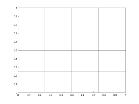
(b)

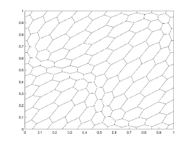
(c)

Figure 1: (A) Triangular, (B) Cartesian and (C) hexagonal initial meshes.

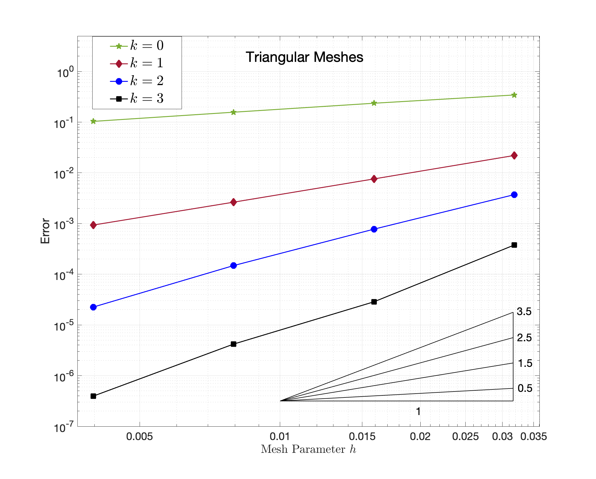
(a)

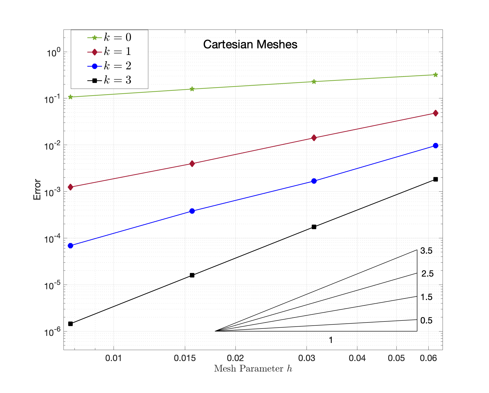
(b)

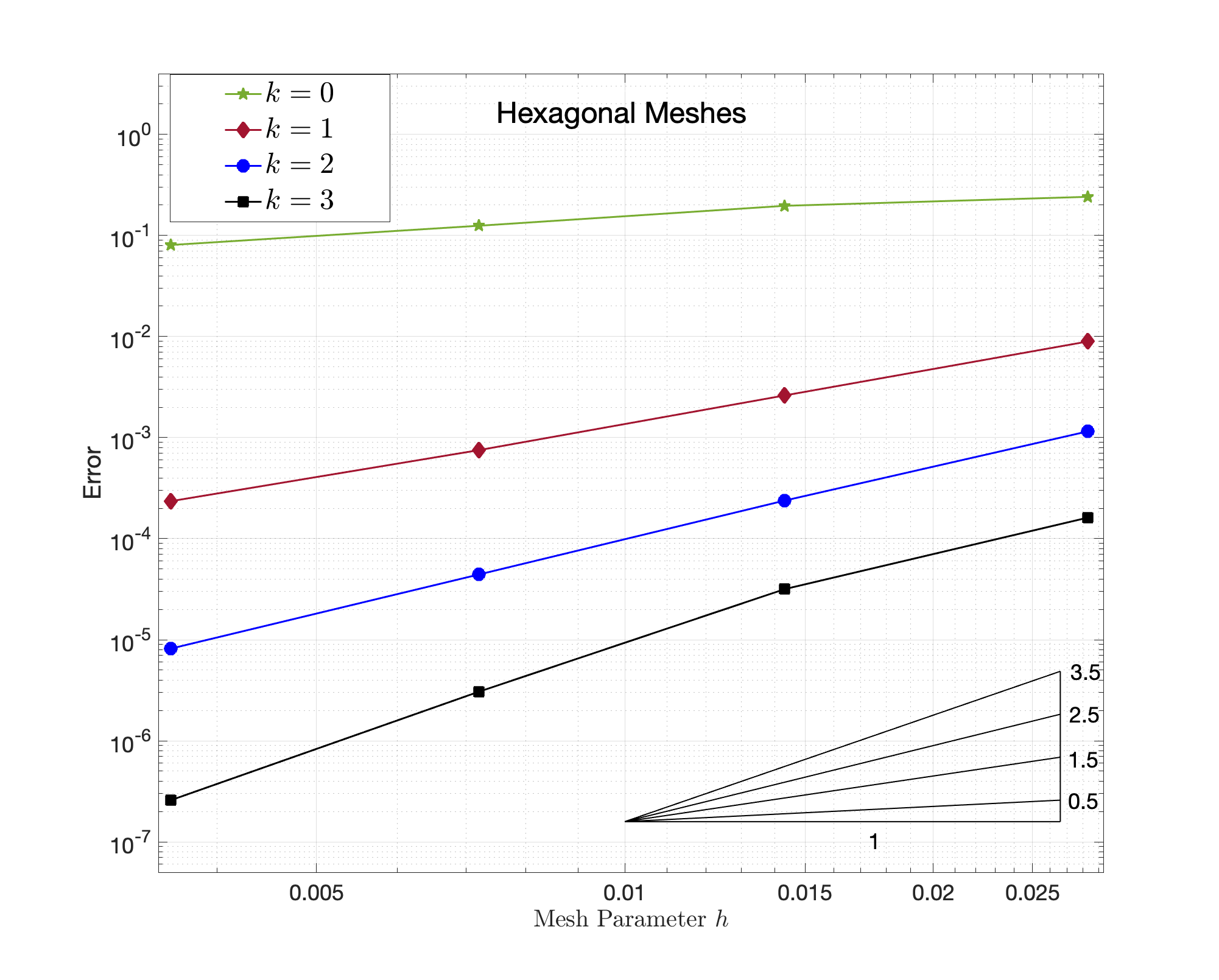
(c)

Figure 2: Convergence histories for the error of Example 5.1 on the (A) triangular, (B) Cartesian, and (C) hexagonal meshes for $\epsilon=10^{-8}$.

Example 5.2 (Boundary layer problem).

Consider the test problem (0.1) for $\epsilon=10^{-2}$ with $\boldsymbol{b}=(1,1)$ and $\sigma=1$. Let the exact solution of velocity and pressure be given by

$$u(x,y)=\begin{bmatrix}2x^{2}y(e^{\lambda(x-1)}-1)^{2}(e^{\lambda(y-1)}-1)^{2}+2x^{2}y^{2}\lambda e^{z(y-1)}(e^{z(x-1)}-1)^{2}(e^{\lambda(y-1)}-1)\\ 2xy^{2}(e^{\lambda(x-1)}-1)^{2}(e^{\lambda(y-1)}-1)^{2}+2x^{2}y^{2}\lambda e^{\lambda(x-1)}(e^{\lambda(x-1)}-1)(e^{\lambda(y-1)}-1)^{2}\end{bmatrix},$$

$$p(x,y)=e^{x+y}-(e-1)^{2},$$

where $\lambda=\frac{1}{2\sqrt{\epsilon}}$.

With the above problem setups, we perform numerical tests on the triangular, Cartesian and hexagonal mesh families as described in the previous Example 5.1. In Figure 3, we plotted the error $\left|\!\left|\!\left|(\underline{\boldsymbol{e}}_{h}^{\boldsymbol{u}},e_{h}^{p})\right|\!\right|\!\right|_{\rm LP}$ as a function of meshsize $h$ for polynomial degrees $k=1,2,3$ with $\epsilon=10^{-2}$. The convergence rates are approximately $h^{k+1/2}$ for $\epsilon=10^{-2}$. Moreover, we observe that the boundary layer problem with $\epsilon\leq 10^{-3}$ or less shows sub-optimal convergence rate as our meshes are not fine enough to capture the layer.

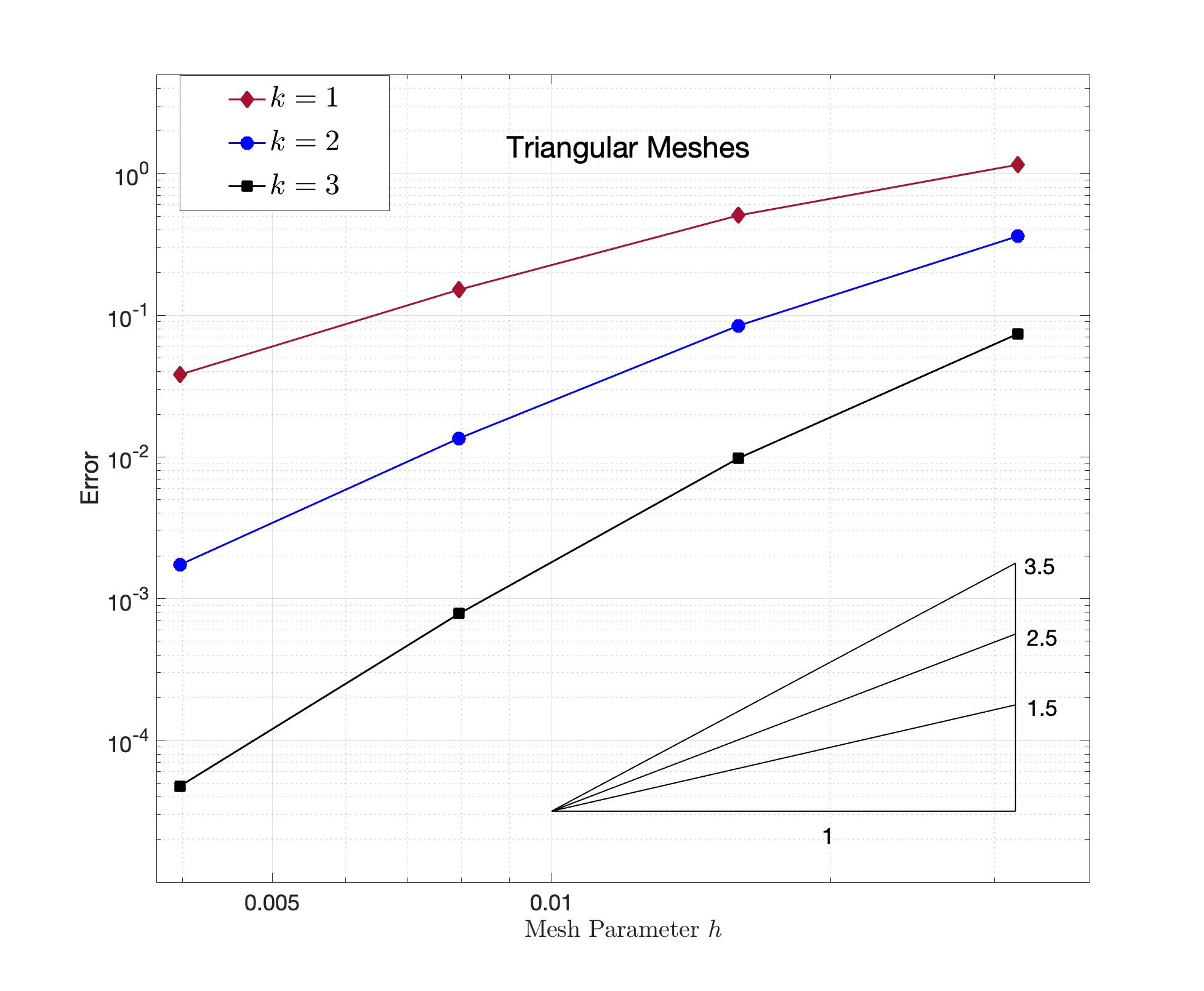
(a)

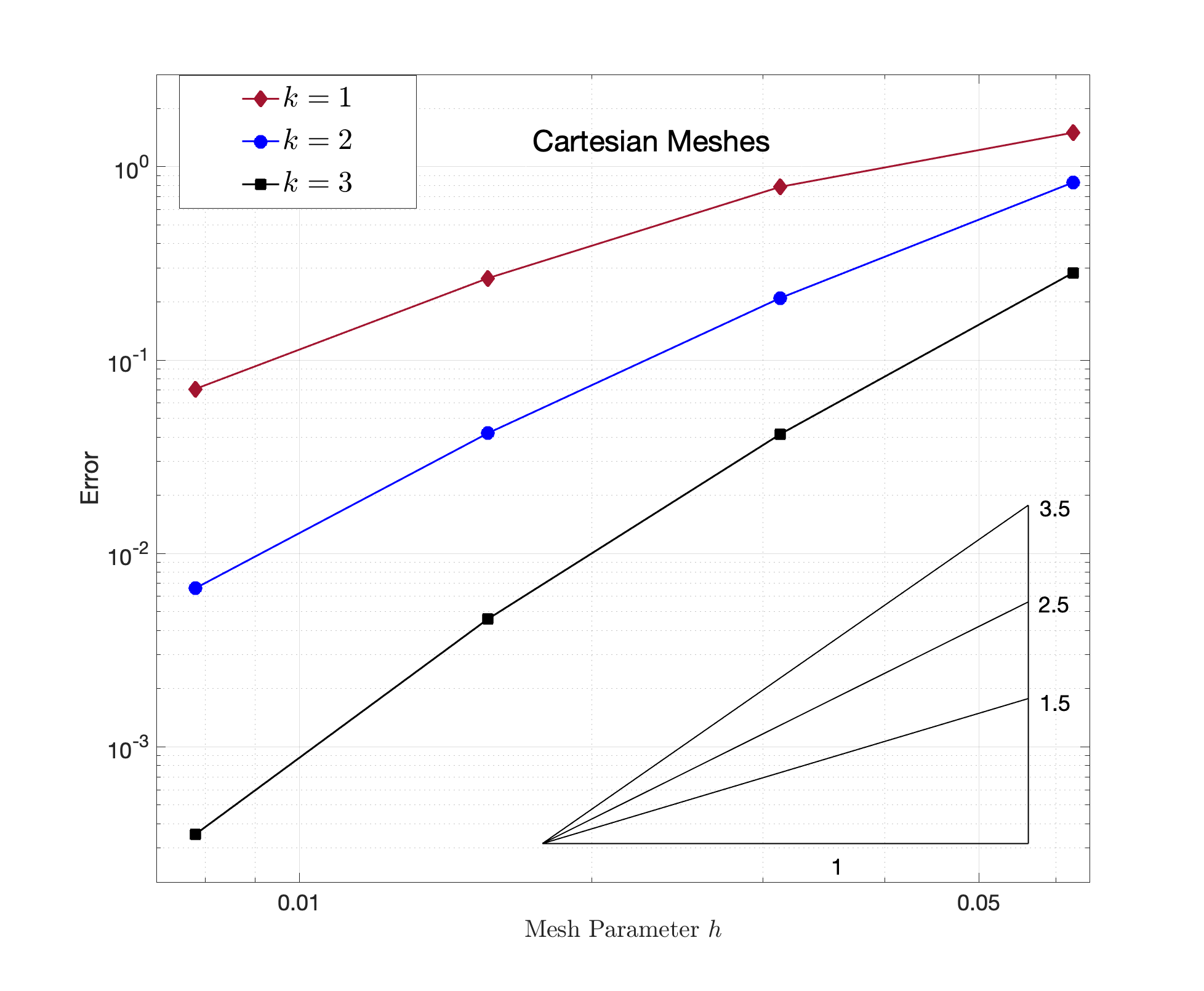
(b)

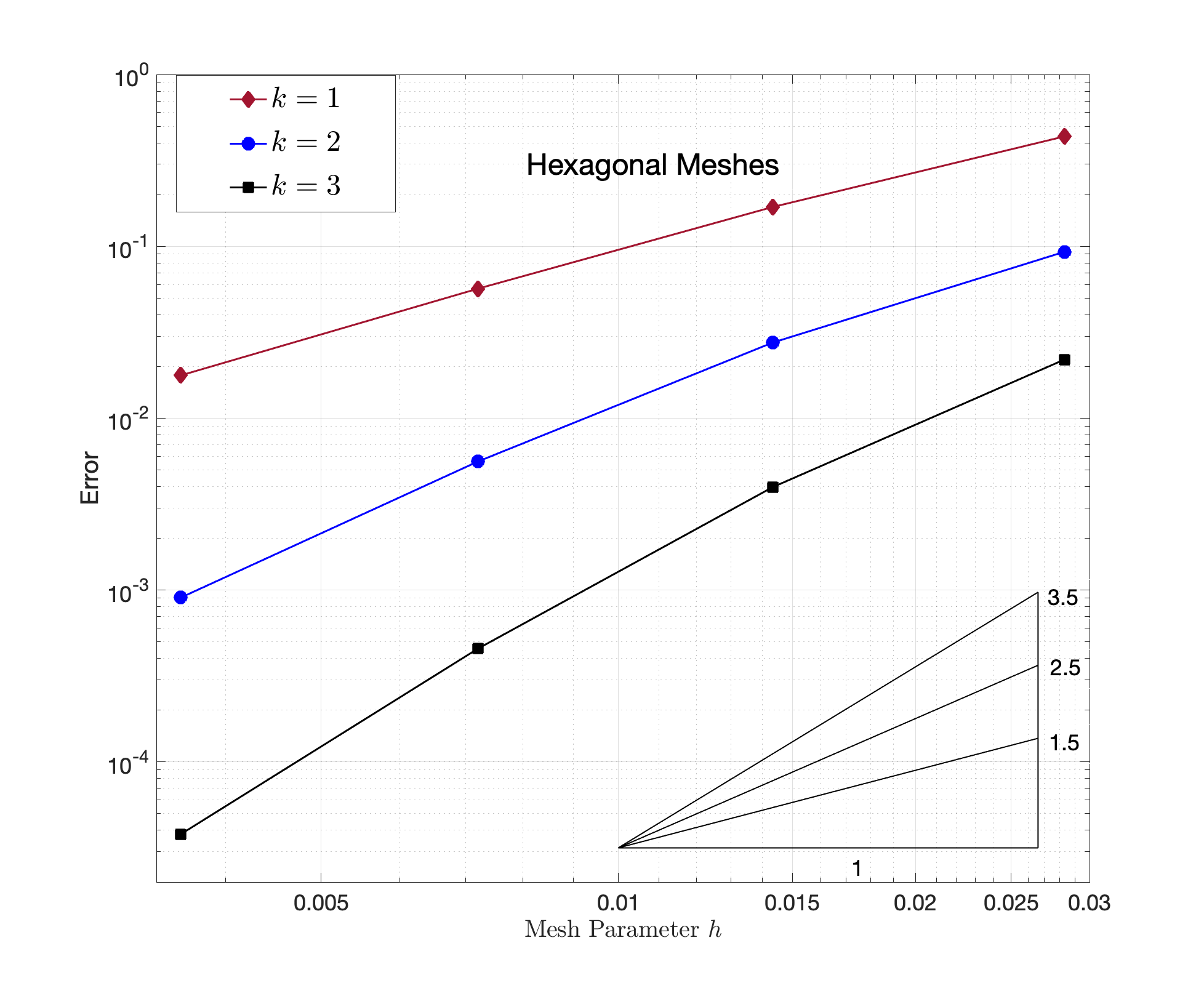
(c)

Figure 3: Convergence histories for the error of Example 5.2 on the (A) triangular, (B) Cartesian, and (C) hexagonal meshes for $\epsilon=10^{-2}$.

6 Conclusions

In this article, we have considered a local projection stabilised Hybrid High-Order method for the Oseen problem. We have proved a strong stability result for our discrete formulation under the SUPG norm. The error analysis shows the optimal order of convergence $(k+1/2)$, assuming that the velocity and the pressure have regularity $H^{k+1}$ globally and $H^{k+2}$ locally. This analysis can be extended to three dimensions with an appropriate change in the mesh structure. The first numerical experiment shows that the optimal order of convergence is achieved. The second example shows that the boundary layer is also captured. It is our presumption that the issue of suboptimal convergence rate in example 5.2 with $\epsilon\leq 10^{-3}$ can be resolved using an adaptive approach. This will be considered in future work.

Acknowledgements
The first author acknowledges the DST-SERB-MATRICS grant MTR/2023/000681 for financial support.

7 Appendix

Note that the global divergence reconstruction operator $D_{h}^{k}$ defined as $D_{h}^{k}\rvert_{T}=D_{T}^{k}$ produces globally $L^{2}_{0}(\Omega)$ function. This can be checked simply by taking $p=1$ on each cell $T\in\mathcal{T}_{h}$ and using the fact that $\boldsymbol{v}_{F}=0$ on the boundary edges for a hybrid function $\underline{\boldsymbol{v}}_{h}=(\underline{\boldsymbol{v}}_{T},\underline{\boldsymbol{v}}_{F})\in\underline{\boldsymbol{U}}_{h,0}^{k}$.

$$\sum_{T\in\mathcal{T}_{h}}(D_{T}^{k}\underline{\boldsymbol{v}}_{T},1)_{T}=\sum_{T\in\mathcal{T}_{h}}\sum_{F\in\mathcal{F}_{T}}(\boldsymbol{v}_{F}\cdot\boldsymbol{n},1)_{F}=0.$$

Along with this $D_{h}^{k}$ is also a continuous linear surjective operator from $\underline{\boldsymbol{U}}_{h,0}^{k}$ to $P_{h}^{k}$. Moreover, we have the following lemma.

Lemma 7.1.

There exists $\alpha>0$ independent of meshsize such that for all $p_{h}\in P_{h}^{k}$ we have the following

$$\sup_{\underline{\boldsymbol{v}}_{h}\in\underline{\boldsymbol{U}}_{0,h}^{k}}\frac{B_{h}(\underline{\boldsymbol{v}}_{h},p_{h})}{\left\|\underline{\boldsymbol{v}}_{h}\right\|_{{\rm dG}}+(\sum_{T\in\mathcal{T}_{h}}\left\|\underline{\boldsymbol{v}}_{T}\right\|^{2}_{T})^{1/2}}\geq\alpha\left\|p_{h}\right\|.$$ (7.1)

Proof.

It is well known that the velocity/pressure pair $[H^{1}_{0}(\Omega)]^{2}/L^{2}_{0}(\Omega)$ is stable and the continuous divergence operator is surjective. Therefore, for any $p_{h}\in P_{h}^{k}$ one can have a unique $\boldsymbol{v}\in\boldsymbol{V}$ such that $\left\|\boldsymbol{v}\right\|_{1}\leq C\left\|p_{h}\right\|$ and ${\rm div~{}}\boldsymbol{v}=-p_{h}$. Using this and the relation $\pi_{T}^{k}({\rm div~{}}\boldsymbol{v})=D_{T}^{k}(\underline{\boldsymbol{I}}_{h}(\boldsymbol{v}))$ we get

$$\left\|p_{h}\right\|^{2}_{\Omega}=(-{\rm div~{}}\boldsymbol{v},p_{h})_{\Omega}=B_{h}(\underline{\boldsymbol{I}}_{h}^{k}(\boldsymbol{v}),p_{h})$$ (7.2)

Moreover, using the approximation properties of $\pi_{T}^{k}$ and $\pi_{F}^{k}$ we have

$$\left\|\underline{\boldsymbol{I}}_{h}(\boldsymbol{v})\right\|^{2}_{{\rm dG}}+\sum_{T\in\mathcal{T}_{h}}\left\|\underline{\boldsymbol{I}}_{T}(\boldsymbol{v})\right\|^{2}_{T}$$

$$=\sum_{T\in\mathcal{T}_{h}}\Big{(}\left\|\underline{\boldsymbol{I}}_{T}(\boldsymbol{v})\right\|^{2}_{T}+\left\|\nabla\underline{\boldsymbol{I}}_{T}(\boldsymbol{v})\right\|^{2}_{T}+\sum_{F\in\mathcal{F}_{T}}\int_{F}\frac{1}{h_{F}}(\pi_{F}^{k}(\boldsymbol{v})-\pi_{T}^{k}(\boldsymbol{v}))^{2}\Big{)}$$

$$\leq C\left\|\boldsymbol{v}\right\|_{1}^{2}\leq C\left\|p_{h}\right\|^{2}$$ (7.3)

Using the relations (7.2) and (7) we arrive at (7.1) with $\alpha=1/C$. ∎

Since $P_{h}^{k}$ is a reflexive space and the discrete divergence operator $D_{h}$ is surjective, the converse of the Lemma A.42 in [41] says that for any $p_{h}\in P_{h}^{k}$ there exists $\underline{\boldsymbol{v}}_{h}\in\underline{\boldsymbol{U}}_{0,h}^{k}$ such that

$$D_{h}^{k}(\underline{\boldsymbol{v}}_{h})=p_{h}\quad\text{and}\quad\left\|\underline{\boldsymbol{v}}_{h}\right\|_{{\rm dG}}^{2}+\sum_{T\in\mathcal{T}_{h}}\left\|\boldsymbol{v}\right\|^{2}_{T}\leq C\left\|p_{h}\right\|^{2},~{}\text{C depends on }\Omega.$$ (7.4)

References

• [1] J. Aghili and D. A. Di Pietro, An advection-robust hybrid high-order method for the Oseen problem, J. Sci. Comput., 77 (2018), pp. 1310–1338.
• [2] R. Araya, C. Harder, D. Paredes, and F. Valentin, Multiscale hybrid-mixed method, SIAM J. Numer. Anal., 51 (2013), pp. 3505–3531.
• [3] R. Becker and M. Braack, A finite element pressure gradient stabilization for the Stokes equations based on local projections, Calcolo, 38 (2001), pp. 173–199.
• [4] R. Becker and M. Braack, A two-level stabilization scheme for the Navier-Stokes equations, in Numerical mathematics and advanced applications, Springer, Berlin, 2004, pp. 123–130.
• [5] L. Beirão da Veiga, F. Brezzi, A. Cangiani, G. Manzini, L. D. Marini, and A. Russo, Basic principles of virtual element methods, Math. Models Methods Appl. Sci., 23 (2013), pp. 199–214.
• [6] L. Beirão da Veiga, F. Brezzi, and L. D. Marini, Virtual elements for linear elasticity problems, SIAM J. Numer. Anal., 51 (2013), pp. 794–812.
• [7] S. Berrone, A. Borio, and G. Manzini, SUPG stabilization for the nonconforming virtual element method for advection-diffusion-reaction equations, Comput. Methods Appl. Mech. Engrg., 340 (2018), pp. 500–529.
• [8] R. Biswas, A. K. Dond, and T. Gudi, Edge patch-wise local projection stabilized nonconforming fem for the oseen problem, Computational Methods in Applied Mathematics, 19 (2019), pp. 189–214.
• [9] J. Bonelle and A. Ern, Analysis of compatible discrete operator schemes for elliptic problems on polyhedral meshes, ESAIM Math. Model. Numer. Anal., 48 (2014), pp. 553–581.
• [10] M. Braack and E. Burman, Local projection stabilization for the Oseen problem and its interpretation as a variational multiscale method, SIAM J. Numer. Anal., 43 (2006), pp. 2544–2566.
• [11] M. Braack and T. Richter, Solutions of 3d navier–stokes benchmark problems with adaptive finite elements, Computers and Fluids, 35 (2006), pp. 372–392.
• [12] M. Braack and T. Richter, Stabilized finite elements for 3D reactive flows, Internat. J. Numer. Methods Fluids, 51 (2006), pp. 981–999.
• [13] F. Brezzi, R. S. Falk, and L. D. Marini, Basic principles of mixed virtual element methods, ESAIM Math. Model. Numer. Anal., 48 (2014), pp. 1227–1240.
• [14] F. Brezzi, K. Lipnikov, and M. Shashkov, Convergence of the mimetic finite difference method for diffusion problems on polyhedral meshes, SIAM J. Numer. Anal., 43 (2005), pp. 1872–1896.
• [15] F. Brezzi, K. Lipnikov, M. Shashkov, and V. Simoncini, A new discretization methodology for diffusion problems on generalized polyhedral meshes, Comput. Methods Appl. Mech. Engrg., 196 (2007), pp. 3682–3692.
• [16] F. Brezzi, K. Lipnikov, and V. Simoncini, A family of mimetic finite difference methods on polygonal and polyhedral meshes, Math. Models Methods Appl. Sci., 15 (2005), pp. 1533–1551.
• [17] A. N. Brooks and T. J. R. Hughes, Streamline upwind/Petrov-Galerkin formulations for convection dominated flows with particular emphasis on the incompressible Navier-Stokes equations, Comput. Methods Appl. Mech. Engrg., 32 (1982), pp. 199–259. FENOMECH ”81, Part I (Stuttgart, 1981).
• [18] E. Burman and A. Ern, An unfitted hybrid high-order method for elliptic interface problems, SIAM J. Numer. Anal., 56 (2018), pp. 1525–1546.
• [19] A. Cesmelioglu, B. Cockburn, N. C. Nguyen, and J. Peraire, Analysis of HDG methods for Oseen equations, J. Sci. Comput., 55 (2013), pp. 392–431.
• [20] M. Cicuttin, D. A. Di Pietro, and A. Ern, Implementation of discontinuous skeletal methods on arbitrary-dimensional, polytopal meshes using generic programming, J. Comput. Appl. Math., 344 (2018), pp. 852–874.
• [21] M. Cicuttin, A. Ern, and T. Gudi, Hybrid high-order methods for the elliptic obstacle problem, J. Sci. Comput., 83 (2020), pp. Paper No. 8, 18.
• [22] B. Cockburn, D. A. Di Pietro, and A. Ern, Bridging the hybrid high-order and hybridizable discontinuous Galerkin methods, ESAIM Math. Model. Numer. Anal., 50 (2016), pp. 635–650.
• [23] B. Cockburn, B. Dong, J. Guzmán, M. Restelli, and R. Sacco, A hybridizable discontinuous Galerkin method for steady-state convection-diffusion-reaction problems, SIAM J. Sci. Comput., 31 (2009), pp. 3827–3846.
• [24] B. Cockburn, J. Gopalakrishnan, and R. Lazarov, Unified hybridization of discontinuous Galerkin, mixed, and continuous Galerkin methods for second order elliptic problems, SIAM J. Numer. Anal., 47 (2009), pp. 1319–1365.
• [25] D. A. Di Pietro and J. Droniou, The Hybrid High-Order Method for Polytopal Meshes: Design, Analysis, and Applications, Springer International Publishing, 2020.
• [26] D. A. Di Pietro, J. Droniou, and A. Ern, A discontinuous-skeletal method for advection-diffusion-reaction on general meshes, SIAM J. Numer. Anal., 53 (2015), pp. 2135–2157.
• [27] D. A. Di Pietro, J. Droniou, and G. Manzini, Discontinuous skeletal gradient discretisation methods on polytopal meshes, J. Comput. Phys., 355 (2018), pp. 397–425.
• [28] D. A. Di Pietro and A. Ern, Mathematical aspects of discontinuous Galerkin methods, vol. 69 of Mathématiques & Applications (Berlin) [Mathematics & Applications], Springer, Heidelberg, 2012.
• [29] D. A. Di Pietro and A. Ern, A hybrid high-order locking-free method for linear elasticity on general meshes, Comput. Methods Appl. Mech. Engrg., 283 (2015), pp. 1–21.
• [30] D. A. Di Pietro, A. Ern, and S. Lemaire, An arbitrary-order and compact-stencil discretization of diffusion on general meshes based on local reconstruction operators, Comput. Methods Appl. Math., 14 (2014), pp. 461–472.
• [31] D. A. Di Pietro, A. Ern, A. Linke, and F. Schieweck, A discontinuous skeletal method for the viscosity-dependent Stokes problem, Comput. Methods Appl. Mech. Engrg., 306 (2016), pp. 175–195.
• [32] D. A. Di Pietro and S. Krell, A hybrid high-order method for the steady incompressible Navier-Stokes problem, J. Sci. Comput., 74 (2018), pp. 1677–1705.
• [33] D. A. Di Pietro and S. Lemaire, An extension of the Crouzeix-Raviart space to general meshes with application to quasi-incompressible linear elasticity and Stokes flow, Math. Comp., 84 (2015), pp. 1–31.
• [34] A. K. Dond and T. Gudi, Patch-wise local projection stabilized finite element methods for convection-diffusion-reaction problems, Numer. Methods Partial Differential Equations, 35 (2019), pp. 638–663.
• [35] J. Droniou, Finite volume schemes for diffusion equations: introduction to and review of modern methods, Math. Models Methods Appl. Sci., 24 (2014), pp. 1575–1619.
• [36] J. Droniou and R. Eymard, A mixed finite volume scheme for anisotropic diffusion problems on any grid, Numer. Math., 105 (2006), pp. 35–71.
• [37] J. Droniou, R. Eymard, T. Gallouët, C. Guichard, and R. Herbin, The gradient discretisation method, vol. 82 of Mathématiques & Applications (Berlin) [Mathematics & Applications], Springer, Cham, 2018.
• [38] J. Droniou, R. Eymard, T. Gallouët, and R. Herbin, A unified approach to mimetic finite difference, hybrid finite volume and mixed finite volume methods, Math. Models Methods Appl. Sci., 20 (2010), pp. 265–295.
• [39]  , A unified approach to mimetic finite difference, hybrid finite volume and mixed finite volume methods, Math. Models Methods Appl. Sci., 20 (2010), pp. 265–295.
• [40] J. Droniou, R. Eymard, and R. Herbin, Gradient schemes: generic tools for the numerical analysis of diffusion equations, ESAIM Math. Model. Numer. Anal., 50 (2016), pp. 749–781.
• [41] A. Ern and J.-L. Guermond, Theory and practice of finite elements, vol. 159 of Applied Mathematical Sciences, Springer-Verlag, New York, 2004.
• [42] R. Eymard, T. Gallouët, and R. Herbin, Discretization of heterogeneous and anisotropic diffusion problems on general nonconforming meshes SUSHI: a scheme using stabilization and hybrid interfaces, IMA J. Numer. Anal., 30 (2010), pp. 1009–1043.
• [43] V. Girault and P.-A. Raviart, Finite element methods for Navier-Stokes equations, vol. 5 of Springer Series in Computational Mathematics, Springer-Verlag, Berlin, 1986. Theory and algorithms.
• [44] T. Gudi, G. Mallik, and T. Pramanick, A hybrid high-order method for quasilinear elliptic problems of nonmonotone type, Accepted in SIAM J. Numer. Anal., (2022).
• [45] R. Herbin and F. Hubert, Benchmark on discretization schemes for anisotropic diffusion problems on general grids, in Finite volumes for complex applications V, John Wiley & Sons, 2008, pp. 659–692.
• [46] P. Knobloch, A generalization of the local projection stabilization for convection-diffusion-reaction equations, SIAM J. Numer. Anal., 48 (2010), pp. 659–680.
• [47] P. Knobloch and L. Tobiska, Improved stability and error analysis for a class of local projection stabilizations applied to the Oseen problem, Numer. Methods Partial Differential Equations, 29 (2013), pp. 206–225.
• [48] Y. Kuznetsov, K. Lipnikov, and M. Shashkov, The mimetic finite difference method on polygonal meshes for diffusion-type problems, Comput. Geosci., 8 (2004), pp. 301–324 (2005).
• [49] S. Lemaire, Bridging the hybrid high-order and virtual element methods, IMA J. Numer. Anal., 41 (2021), pp. 549–593.
• [50] Y. Li, M. Feng, and Y. Luo, A new local projection stabilization virtual element method for the Oseen problem on polygonal meshes, Adv. Comput. Math., 48 (2022), p. Paper No. 30.
• [51] L. Mu, J. Wang, and X. Ye, Weak Galerkin finite element methods on polytopal meshes, Int. J. Numer. Anal. Model., 12 (2015), pp. 31–53.
• [52] H.-G. Roos, M. Stynes, and L. Tobiska, Robust numerical methods for singularly perturbed differential equations, vol. 24 of Springer Series in Computational Mathematics, Springer-Verlag, Berlin, second ed., 2008. Convection-diffusion-reaction and flow problems.
• [53] L. Tobiska and R. Verfürth, Analysis of a streamline diffusion finite element method for the Stokes and Navier-Stokes equations, SIAM J. Numer. Anal., 33 (1996), pp. 107–127.
• [54] J. Wang and X. Ye, A weak Galerkin finite element method for second-order elliptic problems, J. Comput. Appl. Math., 241 (2013), pp. 103–115.
• [55]  , A weak Galerkin mixed finite element method for second order elliptic problems, Math. Comp., 83 (2014), pp. 2101–2126.