Discounted Adaptive Online Prediction

Abstract

Online learning is not always about memorizing everything. Since the future can be statistically very different from the past, a critical challenge is to gracefully forget the history while new data comes in. To formalize this intuition, we revisit the classical notion of discounted regret using recently developed techniques in adaptive online learning. Our main result is a new algorithm that adapts to the complexity of both the loss sequence and the comparator, improving the widespread non-adaptive algorithm – gradient descent with a constant learning rate. In particular, our theoretical guarantee does not require any structural assumption beyond convexity, and the algorithm is provably robust to suboptimal hyperparameter tuning. We further demonstrate such benefits through online conformal prediction, a downstream online learning task with set-membership decisions.

1 Introduction

A typical workflow of sequential decision making consists of two stages: offline design and online fine-tuning. The offline stage gives us an initial policy to work with, utilizing a variety of priors such as domain knowledge, offline dataset and inductive bias. The online stage corrects the time-dependent imperfection of such priors, by refining the policy using sequentially revealed data. Taking a convex stateless abstraction, we will study the problem as Online Convex Optimization (OCO) [30, 47]. It is a two-person repeated game between us (the player) and an adversarial environment, with the following per-round interaction protocol.

1. We make a prediction $x_{t}\in\mathcal{X}$ using past observations, where $\mathcal{X}$ is a closed and convex subset of $\mathbb{R}^{d}$.

2. The environment picks a convex loss function $l_{t}:\mathcal{X}\rightarrow\mathbb{R}$, arbitrarily depending on our prediction history $x_{1},\ldots,x_{t}$.

3. We observe a subgradient $g_{t}\in\partial l_{t}(x_{t})$ and suffer the loss $l_{t}(x_{t})$.

4. The environment determines whether the game stops or not. If the game stops, let $T$ be the total number of rounds.

Intuitively, $x_{t}$ corresponds to the parameter of a decision making policy, which might be thought as the weight of a machine learning model. The initial prediction $x_{1}$ encodes the offline priors, while the progression of the $x_{t}$ sequence captures the online fine-tuning process. Different from the standard settings of OCO, we do not explicitly assume anything beyond convexity: the domain $\mathcal{X}$ does not need to be bounded, and the loss functions are not necessarily Lipschitz/curved/smooth.

Of particular importance is the performance metric, which ultimately determines the behavior of our prediction algorithm. The default one is to upper-bound the static regret over the entire time horizon [57],

$$\mathrm{Regret}_{T}(l_{1:T},u)\mathrel{\mathop{:}}=\sum_{t=1}^{T}l_{t}(x_{t})-\sum_{t=1}^{T}l_{t}(u),$$ (1)

but quite clearly, its strength hinges on an implicit stationarity assumption on the environment: there has to be a fixed prediction $u\in\mathcal{X}$ called a comparator that works well throughout the game, which is often too good to be true in the online fine-tuning task we aim for. One could consider nonstationary performance metrics instead, most notably the Zinkevich-style dynamic regret [57] and the strongly adaptive regret [21]. Although both of them are nontrivial problems extensively studied in recent theoretical works, associated optimal algorithms require increasing computation per round. This poses a critical barrier for computation-constrained long horizon applications.

Diverging from these approaches, the present work revisits a “legacy” nonstationary performance metric called the discounted regret: with a discount factor $\lambda\in(0,1]$, define

$$\mathrm{Regret}^{\lambda}_{T}(l_{1:T},u)\mathrel{\mathop{:}}=\sum_{t=1}^{T}\lambda^{T-t}\left[{l_{t}(x_{t})-l_{t}(u)}\right].$$ (2)

It is a generalization of the undiscounted Eq.(1), with $\lambda=1$ recovering the latter. Since the weight of the past decays quickly, it is possible to upper-bound such a performance metric while forgetting much of the history. This controls the computational complexity, and meanwhile, the algorithm can stay sufficiently agile.

To further justify the importance of this approach, let us take a closer look at its background. Since discounting is such a natural idea, it is not surprising that the discounted regret was studied in a number of early works, e.g., [12]. Although the community shifted away from it, the associated algorithmic insight has thrived on its own. For example, an extremely prevalent practice in nonstationary decision making (sometimes called continual learning [2]) is Online Gradient Descent (OGD) with constant learning rate (LR). From a theoretical perspective (Section 3.1), if the loss functions $l_{1:T}$ are Lipschitz and the domain $\mathcal{X}$ is bounded, then constant-LR OGD guarantees a minimax optimal upper bound on the discounted regret Eq.(2), rather than the standard undiscounted regret Eq.(1). The latter is deeply associated to convergence, which in turn requires the learning rate to shrink to zero.

The main goal of this paper is to design an adaptive algorithm that further improves this popular OGD baseline. In standard online learning terms [47, Chapter 4.2 and 9], an algorithm is adaptive if its regret bound depends on the complexity of the actual problem instance, rather than its conservative overestimate. Precisely, we study the discounted regret Eq.(2): instead of upper-bounding its worst case value $\sup_{l_{1:T},u}\mathrm{Regret}_{T}^{\lambda}(l_{1:T},u)$ under artificial assumptions, we will upper-bound $\mathrm{Regret}_{T}^{\lambda}(l_{1:T},u)$ itself by a function of both the observed gradients $g_{1},\ldots,g_{T}$ and the comparator $u\in\mathcal{X}$. Such a fine-grained approach ensures that the discounted regret bound of our algorithm is almost never worse than the minimax optimal bound of constant-LR OGD, and can improve the latter when the environment is “easy”, e.g., when the offline priors are good. On the practical side, there is another key strength: our algorithm gradually forgets the past online data but not the offline priors, whereas constant-LR OGD forgets everything altogether.

1.1 Contribution

This paper presents two types of new results, ($i$) discounted online learning theory, and ($ii$) applications in Online Conformal Prediction (OCP).

• First, we consider the OCO problem with discounted regret Eq.(2). Defining the effective time horizon $H=\sum_{t=1}^{T}\lambda^{2(T-t)}$ and the effective gradient variance $V=\sum_{t=1}^{T}\lambda^{2(T-t)}\left\|{g_{t}}\right\|^{2}$, we develop a new algorithm that virtually guarantees (see Theorem 4 for the details)

  $$\mathrm{Regret}^{\lambda}_{T}(l_{1:T},u)\leq\tilde{O}\left({\left\|{u-x_{1}}\right\|\sqrt{V}}\right),$$

  matching an instance-dependent $\Omega(\left\|{u-x_{1}}\right\|\sqrt{V})$ lower bound. In comparison, constant-LR OGD achieves an $O(DG\sqrt{H})$ upper bound assuming $D$-bounded domain and $G$-Lipschitz losses – our result improves that while removing both assumptions.

  The key to our result is a simple rescaling trick, which converts scale-free undiscounted regret bounds to their discounted analogues. In this way, advances in stationary online learning can be exploited quite easily in the general nonstationary setting, which provides a compelling alternative to the standard aggregation approach there (e.g., the meta-expert framework that minimizes the dynamic regret and the strongly adaptive regret, surveyed in Appendix A).

• Second, we move to OCP, a downstream online learning task with confidence set predictions. To combat the distribution shifts commonly found in practice, recent works [27, 28, 10] developed the application of nonstationary OCO algorithms (such as constant-LR OGD) to this setting. The twist is that besides appropriate regret bounds, one has to establish coverage guarantees as well, i.e., bounding the magnitude of the cumulative gradient sum over a sliding time window.

  For this problem, we demonstrate various quantitative strengths of our discounted OCO approach. In particular, the gradient adaptivity in OCO leads to the adaptivity to the targeted miscoverage rate in OCP, and the comparator adaptivity in OCO allows removing the “oracle tuning” assumption from existing works. In terms of the techniques, since our algorithm is built on the Follow the Regularized Leader (FTRL) framework rather than OGD, the associated coverage guarantee follows naturally from the stability of its iterates. Such an FTRL-based analytical strategy could be of independent interest.

Finally, we demonstrate the practicality of our algorithm through OCP experiments.

1.2 Notation

Throughout this paper, $\left\|{\cdot}\right\|$ denotes the Euclidean norm. $\Pi_{\mathcal{X}}(x)$ is the Euclidean projection of $x$ onto a closed convex set $\mathcal{X}$. The diameter of a set $\mathcal{X}$ is $\sup_{x,y\in\mathcal{X}}\left\|{x-y}\right\|$.

For two integers $a\leq b$, $[a:b]$ is the set of all integers $c$ such that $a\leq c\leq b$. The brackets are removed when on the subscript, denoting a tuple with indices in $[a:b]$. If $a>b$, then the product $\prod_{i=a}^{b}\lambda_{i}\mathrel{\mathop{:}}=1$. $0$ represents a zero vector whose dimension depends on the context. $\log$ means natural logarithm.

We define the imaginary error function as $\mathrm{erfi}(x)\mathrel{\mathop{:}}=\int_{0}^{x}\exp(u^{2})du$; this is scaled by $\sqrt{\pi}/2$ from the conventional definition, thus can also be queried from standard software packages like SciPy and JAX.

2 Related work

Discounted regret

Motivated by the intuition that “the recent history is more important than the distant past”, the discounted regret has been studied by a rich line of works [12, 24, 19, 37, 11, 7]. Most of them were before the burst of adaptive online learning, although the under-appreciated [37] presented ideas that foreshadowed some of the later developments. Recently, the study of dynamic regret and strongly adaptive regret has taken over the field of nonstationary online learning, which we summarize in Appendix A. These are indeed very valuable topics, but we believe that the discounted regret could still be a useful alternative, especially due to the associated simplicity and computational efficiency. Through a modern adaptive treatment, we hope to renew the interest of the field in this classical metric, which then benefits downstream applications such as OCP.

Another remark is that discounting on a data stream is tightly connected to filtering and sliding windows in signal processing [46] and theoretical computer science [20]. The relation of our results to such fields could be investigated in future works.

Adaptive online learning

Adaptive OCO in the stationary setting has been mainly studied from two angles. The famous AdaGrad [22, 40] achieves the adaptivity to the loss functions $l_{1:T}$, while parameter-free online learning [51, 42, 43, 26, 54] concerns the adaptivity to the comparator $u$. A number of recent works achieve them both [15, 17, 41, 13, 34, 59], which our work builds on.

Comparison with DL optimizers

As we will show, discounted OCO algorithms employ Exponential Moving Average (EMA) under the hood. This is an important idea in deep learning (DL) optimization, as exemplified by the empirical success of RMSProp [52] and Adam [36], and the enormous literature that tries to explain it. A notable issue here is the appeared mismatch between the two intuitions: DL is usually modeled as a (stationary and non-convex) stochastic optimization problem that requires convergence [49, 38], whereas EMA is employed (at least in discounted OCO algorithms) for the “forgettive and non-convergent” behavior. Reconciling this conflict is an important problem for DL optimization, which this work does not consider. Instead, we focus on the well-posed problem of nonstationary online learning, where non-convergence is indeed necessary.

3 Discounted adaptivity

Setting

We study the OCO problem defined at the beginning of the paper, with a slightly generalized discounted regret. Instead of having a fixed discount factor $\lambda\in(0,1]$ throughout the game, let us consider a sequence of discount factors $\lambda_{1},\ldots,\lambda_{T}\in(0,\infty)$, and the $t$-th one is revealed at the end of the $(t+1)$-th round (for all $t\leq 0$, let $\lambda_{t}=1$). In this setting, the weight of the past can possibly increase. Accordingly, we define the generalized discounted regret as

$$\mathrm{Regret}^{\lambda_{1:T}}_{T}(l_{1:T},u)\mathrel{\mathop{:}}=\sum_{t=1}^{T}\left({\prod_{i=t}^{T-1}\lambda_{i}}\right)\left[{l_{t}(x_{t})-l_{t}(u)}\right],$$ (3)

which recovers Eq.(2) as its fixed-$\lambda<1$ special case. Throughout this paper, we will treat $\lambda_{1:T}$ as part of the problem description and focus on bounding Eq.(3), but in practice, a meta-learning approach might be applied on top to select $\lambda_{1:T}$ online.

3.1 Preliminary

Intuitively, the main difference between the discounted regret Eq.(3) and the standard undiscounted regret Eq.(1) is the effective time horizon. Instead of the maximum length $T$, in the $t$-th round we care about an exponentially weighted look-back window of length

$$H_{t}\mathrel{\mathop{:}}=\sum_{i=1}^{t}\left({\prod_{j=i}^{t-1}\lambda^{2}_{j}}\right),$$ (4)

which is roughly $\min[(1-\lambda^{2})^{-1},T]$ in the fixed-$\lambda$ special case. For later use, we also define the discounted gradient variance $V_{t}$ and the discounted Lipschitz constant $G_{t}$,

$$V_{t}\mathrel{\mathop{:}}=\sum_{i=1}^{t}\left({\prod_{j=i}^{t-1}\lambda_{j}^{2}}\right)\left\|{g_{i}}\right\|^{2},\quad G_{t}\mathrel{\mathop{:}}=\max_{i\in[1:t]}\left({\prod_{j=i}^{t-1}\lambda_{j}}\right)\left\|{g_{i}}\right\|.$$ (5)

A classical wisdom in online learning is that for gradient descent, the learning rates could be set proportional to the inverse square root of the time horizon. Combining it with $H_{t}$ above, it is likely a folklore that non-adaptive OGD can be generalized easily to the discounted setting. Let us make it concrete.

Online Gradient Descent

Consider the OGD update rule: after observing the loss gradient $g_{t}$, we pick a learning rate $\eta_{t}$, take a gradient step and project the update back to the domain $\mathcal{X}$, i.e.,

$$x_{t+1}=\Pi_{\mathcal{X}}\left({x_{t}-\eta_{t}g_{t}}\right).$$

Throughout this section, the initialization $x_{1}$ is fixed at the origin. This is without loss of generality, since a different initialization can be implemented by simply shifting the coordinates. We call an algorithm non-adaptive if its regret bound is on the worst case, $\sup_{l_{1:T},u}\mathrm{Regret}^{\lambda_{1:T}}_{T}(l_{1:T},u)$. This implies that $\eta_{t}$ only depends on the historical discount factors, and our baseline (constant-LR OGD) is the most notable example.

Theorem 1 (Abridged Theorem 6 and 7).

If the loss functions are all $G$-Lipschitz, the diameter of the domain is at most $D$, and the discount factor $\lambda_{t}=\lambda\in(0,1)$, then OGD with a constant learning rate $\eta_{t}=\frac{D}{G}\sqrt{1-\lambda^{2}}$ guarantees for all $T=\Omega(\frac{1}{1-\lambda})$,

$$\sup_{l_{1:T},u}\mathrm{Regret}^{\lambda}_{T}(l_{1:T},u)=O\left({DG\sqrt{H_{T}}}\right).$$

Conversely, fix any variance budget $V\in(0,G^{2}H_{T}]$, and any comparator $u$ such that $u,-u\in\mathcal{X}$. For any algorithm, there exists a loss sequence such that $V_{T}$ defined in Eq.(5) satisfies $V_{T}=V$, and

$$\max\left[{\mathrm{Regret}^{\lambda_{1:T}}_{T}(l_{1:T},u),\mathrm{Regret}^{\lambda_{1:T}}_{T}(l_{1:T},-u)}\right]=\Omega\left({\left\|{u}\right\|\sqrt{V_{T}}}\right).$$

Picking the domain $\mathcal{X}$ as a norm ball centered at the origin, one could see that the worst case bound of constant-LR OGD is optimal under the Lipschitzness and bounded-domain assumptions. Such a result forms the theoretical foundation of this common practice. Meanwhile, there is an instance-dependent gap that illustrates a natural direction to improve the algorithm: removing the supremum, can we directly achieve

$$\mathrm{Regret}^{\lambda_{1:T}}_{T}(l_{1:T},u)=O\left({\left\|{u}\right\|\sqrt{V_{T}}}\right),$$ (6)

without any extra assumption at all? If successful, such a bound will never be worse than the $O(DG\sqrt{H_{T}})$ bound of constant-LR OGD (under the same assumptions), while the algorithm could be agnostic to both $D$ and $G$. This is the key strength of adaptive online learning: without imposing any artificial structural assumption, the algorithm performs as if it knows the “correct” assumption from the beginning.

3.2 Main result

To pursue Eq.(6), our main idea is the following rescaling trick.

• In the undiscounted setting ($\lambda_{t}=1$), Eq.(6) has been almost achieved by a number of recent works [17, 41, 34, 55] modulo necessary residual factors. For any algorithm $\mathcal{A}$ (possibly taken from these works), let $\mathrm{Regret}_{T,\mathcal{A}}(g_{1:T},u)$ denote its undiscounted static regret with respect to linear losses $\left\langle g_{t},\cdot\right\rangle$ and comparator $u$, c.f., Eq.(1).

• Next, consider the discounted regret Eq.(3). We take an aforementioned algorithm $\mathcal{A}$ and apply it to a sequence of surrogate loss gradients $\hat{g}_{1:T}$, where

  $$\hat{g}_{t}=\left({\prod_{i=1}^{t-1}\lambda_{i}^{-1}}\right)g_{t}.$$ (7)

  If $\lambda_{1},\ldots,\lambda_{T}<1$, this amounts to “upweighting” recent losses, or equivalently, “forgetting” older ones. The generated prediction sequence $x_{1:T}$ satisfies a discounted regret bound that scales with $\mathrm{Regret}_{T,\mathcal{A}}\left({\hat{g}_{1:T},u}\right)$, the undiscounted regret of the base algorithm $\mathcal{A}$ on $\hat{g}_{1:T}$.

  $$\mathrm{Regret}^{\lambda_{1:T}}_{T}(l_{1:T},u) =\left({\prod_{t=1}^{T-1}\lambda_{t}}\right)\cdot\sum_{t=1}^{T}\left({\prod_{i=1}^{t-1}\lambda^{-1}_{i}}\right)\left[{l_{t}(x_{t})-l_{t}(u)}\right]$$

  $$\leq\left({\prod_{t=1}^{T-1}\lambda_{t}}\right)\mathrm{Regret}_{T,\mathcal{A}}\left({\hat{g}_{1:T},u}\right).$$ (8)

  This might seem trivially simple, but we will show that using the right base algorithm $\mathcal{A}$ leads to a range of practically desirable properties, which are in our opinion not obvious beforehand.

Within this trick, a particular challenge is that even if all the actual loss functions $l_{t}$ are Lipschitz in a time-uniform manner ($\exists G,s.t.,\max_{t}\left\|{g_{t}}\right\|\leq G$), the surrogate loss functions $\left\langle\hat{g}_{t},\cdot\right\rangle$ are not. Therefore, the base algorithm $\mathcal{A}$ cannot rely on any a priori knowledge or estimate of the time-uniform Lipschitz constant, similar to the classical scale-free property [44]. To make this concrete, we first forego the adaptivity to the comparator $u$ and analyze an example based on the famous AdaGrad [22]. The result is visually appealing, as all the annoying residual factors required by the full generality of our problem (simultaneous adaptivity to both $l_{1:T}$ and $u$) are gone. The algorithm itself will be a building block of our main results.

Gradient adaptive OGD

Proposed for the undiscounted setting, AdaGrad [22] symbolizes OGD with gradient-dependent learning rates. Using it as the base algorithm $\mathcal{A}$ leads to the following RMSProp-like prediction rule and its discounted regret bound.

Theorem 2.

If the diameter of $\mathcal{X}$ is at most $D$, then OGD with learning rate $\eta_{t}=DV_{t}^{-1/2}$ guarantees for all $T\in\mathbb{N}_{+}$ and loss sequence $l_{1:T}$,

$$\sup_{u}\mathrm{Regret}^{\lambda_{1:T}}_{T}(l_{1:T},u)\leq\frac{3}{2}D\sqrt{V_{T}}.$$

As one would hope for, the bound strictly improves constant-LR OGD while matching the lower bound on the $\sqrt{V_{T}}$ dependence. It is tempting to seek an even better learning rate $\eta_{t}$ that improves the remaining $D$ to $\left\|{u}\right\|$, but such a direction leads to a dead end (Remark B.1). To solve this problem, we will resort to the Follow the Regularized Leader (FTRL) framework [47, Chapter 7] instead of OGD. The key intuition [25, 34] is that, FTRL is stronger since it memorizes the initialization, whereas OGD (without extra regularization) does not.

Simultaneous adaptivity

To achieve simultaneous adaptivity to both $l_{1:T}$ and $u$, things can get subtle. As mentioned earlier, there are a number of choices for the base algorithm $\mathcal{A}$. We will adopt the latest version from [59], which offers an important benefit (no explicit $T$-dependence, Remark B.4). Without loss of generality, let us assume the domain $\mathcal{X}=\mathbb{R}^{d}$. The undiscounted algorithm from [59] is surveyed in Appendix B.2 for easier reference.

Overall, our discounted algorithm employs the polar-decomposition technique from [15]: using polar coordinates, predicting $x_{t}\in\mathbb{R}^{d}$ can be decomposed into two independent tasks, learning the good direction $u/\left\|{u}\right\|$ and the good magnitude $\left\|{u}\right\|$. The direction is learned by the RMSProp-like algorithm from Theorem 2, while the magnitude is learned by a discounted variant of the $\mathrm{erfi}$-potential learner [59, Algorithm 1] that operates on the positive real line $[0,\infty)$. This magnitude learner itself will be important for our downstream application, therefore we present its pseudocode as Algorithm 1.

Algorithm 1 1D magnitude learner on $[0,\infty)$.

0:  Hyperparameter $\varepsilon>0$ (default $\varepsilon=1$).

1:  Initialize parameters $v_{1}=0$, $s_{1}=0$, $h_{1}=0$.

2:  for $t=1,2,\ldots$ do

3:     If $h_{t}=0$, define the unprojected prediction $\tilde{x}_{t}=0$. Otherwise, with $\mathrm{erfi}(x)\mathrel{\mathop{:}}=\int_{0}^{x}\exp(u^{2})du$ (which can be queried from SciPy and JAX),

$$\tilde{x}_{t}=\varepsilon\cdot\mathrm{erfi}\left({\frac{s_{t}}{2\sqrt{v_{t}+2h_{t}s_{t}+16h^{2}_{t}}}}\right)-\frac{\varepsilon h_{t}}{\sqrt{v_{t}+2h_{t}s_{t}+16h_{t}^{2}}}\exp\left[{\frac{s_{t}^{2}}{4(v_{t}+2h_{t}s_{t}+16h_{t}^{2})}}\right].$$

4:     Predict $x_{t}=\Pi_{[0,\infty)}\left({\tilde{x}_{t}}\right)$, the projection of $\tilde{x}_{t}$ to the domain $[0,\infty)$.

5:     Receive the 1D loss gradient $g_{t}\in\mathbb{R}$ and the discount factor $\lambda_{t-1}\in(0,\infty)$.

6:      Clip $g_{t}$ by defining $g_{t,\mathrm{clip}}=\Pi_{[-\lambda_{t-1}h_{t},\lambda_{t-1}h_{t}]}\left({g_{t}}\right)$, and update $h_{t+1}=\max\left({\lambda_{t-1}h_{t},\left|{g_{t}}\right|}\right)$.

7:      If $g_{t,\mathrm{clip}}\tilde{x}_{t}<g_{t,\mathrm{clip}}x_{t}$, define a surrogate loss gradient $\tilde{g}_{t,\mathrm{clip}}=0$. Otherwise, $\tilde{g}_{t,\mathrm{clip}}=g_{t,\mathrm{clip}}$.

8:     Update $v_{t+1}=\lambda_{t-1}^{2}v_{t}+\tilde{g}^{2}_{t,\mathrm{clip}}$, $s_{t+1}=\lambda_{t-1}s_{t}-\tilde{g}_{t,\mathrm{clip}}$.

9:  end for

Algorithm 1 has the following intuition. At its center is a special instance of FTRL, which generates the prediction $x_{t}$ using the discounted gradient variance $v_{t}$, the discounted gradient sum $s_{t}$, and the discounted Lipschitz constant $h_{t}$. Complementing this core component, two additional ideas are applied to fix certain technical problems: ($i$) the unconstrained-to-constrained reduction from [15, 18], and ($ii$) the hint-and-clipping technique from [17]. The readers are referred to Appendix B.2 for a detailed explanation. The point is that understanding the inner workings of the algorithm is not strictly necessary to proceed: we treat the result from [59] as a black box and wrap it using the rescaling trick. In summary, this yields the following theorem proved in Appendix B.3.

Theorem 3.

Given any hyperparameter $\varepsilon>0$, Algorithm 1 guarantees for all time horizon $T\in\mathbb{N}_{+}$, loss sequence $l_{1:T}$, comparator $u\in[0,\infty)$ and stability window length $\tau\in[1:T]$,

$$\mathrm{Regret}^{\lambda_{1:T}}_{T}(l_{1:T},u)\leq\varepsilon\sqrt{V_{T}+2G_{T}S+16G_{T}^{2}}+u\left({S+G_{T}}\right)+\left({\max_{t\in[T-\tau+1:T]}x_{t}}\right)G_{T}+\left({\prod_{t=T-\tau}^{T-1}\lambda_{t}}\right)\left({\max_{t\in[1:T-\tau]}x_{t}}\right)G_{T-\tau},$$

where

$$S=8G_{T}\left({1+\sqrt{\log(2u\varepsilon^{-1}+1)}}\right)^{2}+2\sqrt{V_{T}+16G_{T}^{2}}\left({1+\sqrt{\log(2u\varepsilon^{-1}+1)}}\right).$$

This result might seem a bit intimidating, so let us take a few steps to interpret it. In particular, we want to justify the appropriate asymptotic regime to consider ($V_{T}\gg G_{T}^{2}$ and $u\gg\varepsilon$), such that our main result on $\mathbb{R}^{d}$ (Theorem 4) can use the big-Oh notation to improve clarity.

• First, one would typically expect $V_{T}\gg G_{T}^{2}$, since when $\lambda_{t}=\lambda\in(0,1)$ and $\left|{g_{t}}\right|=G$ for all $t$, we have $G_{T}=G$ and $V_{T}=H_{T}G^{2}\approx(1-\lambda^{2})^{-1}G^{2}$. As long as the discount factor $\lambda_{t}$ is close enough to $1$, the condition $V_{T}\gg G_{T}^{2}$ is likely to hold for general/practical gradient sequences as well.

• Second, the hyperparameter $\varepsilon$ serves as a prior guess of the comparator $u$. If the guess is correct ($\varepsilon=u$), then by assuming $V_{T}\gg G_{T}^{2}$ and $\max_{t\in[1:T]}x_{t}=O(u)$ (roughly speaking, the predictions are stable), the regret bound becomes

  $$\mathrm{Regret}^{\lambda_{1:T}}_{T}(l_{1:T},u)=O\left({u\sqrt{V_{T}}}\right),$$ (9)

  exactly matching the lower bound. Realistically such an “oracle tuning” is illegal, since $\varepsilon$ is selected at the beginning of the game, while reasonable comparators $u$ are hidden before all the loss functions are revealed. This is where our algorithm truly shines: as long as $\varepsilon$ is moderately small, i.e., $O(u)$, we would have the $O(uS)$ term dominating the regret bound, which only suffers a multiplicative logarithmic penalty relative to the impossible oracle-optimal rate Eq.(9). In comparison, it is well-known that the regret bound of constant-LR OGD with learning rate $\eta$ depends polynomially on $\eta$ and $\eta^{-1}$ (c.f., the proof of Theorem 6), which means our algorithm is provably more robust to suboptimal hyperparameter tuning.

• Third, we explain the use of $\tau$. In nonstationary environments, the range of $x_{t}$ can vary significantly over time, therefore a time-uniform characterization of its stability ($\max_{t\in[1:T]}x_{t}$, Remark B.2) could be overly conservative. We use a stability window of arbitrary length $\tau$ to divide the time horizon into two parts: the earlier part is forgotten rapidly (due to the $\prod_{t=T-\tau}^{T-1}\lambda_{t}$ multiplier), so only the later part really matters.

Example 1.

Suppose again that $\lambda_{t}=\lambda\in(0,1)$. If $\lambda\approx 1$, the “forgetting” multiplier can be approximated by

$$\prod_{t=T-\tau}^{T-1}\lambda_{t}=\lambda^{\tau}=\lambda^{\frac{1}{1-\lambda}\cdot(1-\lambda)\tau}\approx e^{(\lambda-1)\tau}.$$ (Lemma B.1)

Consider $\lambda=0.99$ for example: $\tau=700$ ensures $\lambda^{\tau}\approx e^{-7}<10^{-3}$. That is, if the past range of $x_{t}$ is negligible after a $10^{-3}$-attenuation, then our regret bound only depends on the “localized stability” $\max_{t\in[T-699,T]}x_{t}$ evaluated in the recent 700 rounds, which is a small fraction in (let us say) $T\approx\textrm{million}$. More intuitively, it means “past mistakes do not matter”.

Given the 1D magnitude learner and its guarantee, the extension to $\mathbb{R}^{d}$ is now standard [15]. We defer the pseudocode to Appendix B.3.

Theorem 4 (Main result).

Given any hyperparameter $\varepsilon>0$, Algorithm 3 in Appendix B.3 guarantees for all $T\in\mathbb{N}_{+}$, loss gradients $g_{1:T}$ and comparator $u\in\mathbb{R}^{d}$,

$$\mathrm{Regret}^{\lambda_{1:T}}_{T}(l_{1:T},u)\leq O\left({\left\|{u}\right\|\sqrt{V_{T}\log(\left\|{u}\right\|\varepsilon^{-1})}\vee\left\|{u}\right\|G_{T}\log(\left\|{u}\right\|\varepsilon^{-1})}\right)+\left({\max_{t\in[1:T]}x_{t}}\right)G_{T},$$

where $O(\cdot)$ is in the regime of large $V_{T}$ $(V_{T}\gg G_{T})$ and large $\left\|{u}\right\|$ $(\left\|{u}\right\|\gg\varepsilon)$. Furthermore, for $u=0$,

$$\mathrm{Regret}^{\lambda_{1:T}}_{T}(l_{1:T},0)\leq O\left({\varepsilon\sqrt{V_{T}}}\right)+\left({\max_{t\in[1:T]}x_{t}}\right)G_{T}.$$

Similar to Theorem 3, the iterate stability term can be split into two parts using an arbitrary $\tau$. The important message is that if the iterates are indeed stable ($\max_{t\in[1:T]}x_{t}=O(\left\|{u}\right\|)$) and we suppress all the logarithmic factors with $\tilde{O}(\cdot)$, then

$$\mathrm{Regret}^{\lambda_{1:T}}_{T}(l_{1:T},u)\leq\tilde{O}\left({\left\|{u}\right\|\sqrt{V_{T}}}\right).$$

It matches the lower bound and improves all the aforementioned algorithms. Granted, there are several nuances in this statement, but they are in general necessary even in the undiscounted special case [47, Chapter 9].

Finally, we summarize a range of practical strengths. As shown earlier, the proposed algorithm is robust to hyperparameter tuning. Observations and mistakes from the distant past (which are possibly misleading for the future) are appropriately forgotten, such that the algorithm runs “consistently” over its lifetime. Compared to the typical aggregation framework in nonstationary online learning [21, 58], our algorithm runs faster and never explicitly restarts (although we require given discount factors to “softly” restart). In addition, compared to constant-LR OGD that also tries to minimize the discounted regret, our algorithm makes a better use of the offline knowledge – this is so important that we have to discuss it further.

On the initialization

So far we have fixed the initialization $x_{1}$ to $0$. This makes the bounds cleaner but hides a crucial consideration. Suppose we have a ML model that “almost” explains the environment, except just a small amount of noise. Formulated as OCO, it could mean that the optimal prediction sequence $x^{*}_{t}\in\operatorname*{arg\,min}_{x}l_{t}(x)$ satisfies

$$x^{*}_{t}=\bar{x}+\delta_{t},$$

where the time-invariant $\bar{x}$ can be obtained through offline pre-training, and the noise $\delta_{t}$ is small and only revealed online. Naturally, our algorithm could initialize at $x_{1}=\bar{x}$, such that the discounted regret bound becomes $\tilde{O}\left({\left\|{u-\bar{x}}\right\|\sqrt{V_{T}}}\right)$. If the noise $\delta_{t}\approx\delta$ over a sufficiently long look-back window at $T$, then with respect to $u=\bar{x}+\delta$ (which approximates the optimal prediction sequence $\{x^{*}_{t}\}$), our regret is simply $\tilde{O}\left({\left\|{\delta}\right\|\sqrt{V_{T}}}\right)$. In other words, our online prediction performance nicely scales with the accuracy of the pre-trained model over sliding time windows.

In contrast, even if initialized properly, constant-LR OGD does not exhibit solid theoretical improvement. This is fundamentally related to FTRL versus OGD: through the incremental steps, OGD quickly loses track of everything in the past, while our algorithm has a “regularization module” that always remembers the initialization (even though past gradients are forgotten).

4 Online conformal prediction

Next, we consider an application that complements the theory. Conformal prediction [53] is a framework that quantifies the uncertainty of black box ML models. We study its online version [27, 6, 28, 56, 10], where no statistical assumptions (e.g., exchangeability) are imposed at all. Our setting follows the nicely written [10, Section 2], and the readers are referred to [1, 50] for additional background.

4.1 Preliminary

Similar to OCO, OCP is again a two-person repeated game. Let a constant $\alpha\in(0,1)$ be the targeted miscoverage rate fixed before the game starts. At the beginning of the $t$-th round, we receive a set-valued function $\mathcal{C}_{t}:\mathbb{R}_{\geq 0}\rightarrow 2^{\mathcal{Y}}$ mapping any radius parameter $r\in[0,\infty)$ to a subset $\mathcal{C}_{t}(r)$ of the label space $\mathcal{Y}$. The $\mathcal{C}_{t}$ function is nested: for any $r^{\prime}>r$, we have $\mathcal{C}_{t}(r)\subset\mathcal{C}_{t}(r^{\prime})\subset\mathcal{Y}$. Then,

1. We pick a radius parameter $r_{t}\in[0,\infty)$ and output the prediction set $\mathcal{C}_{t}(r_{t})$.

2. The environment reveals the optimal radius $r^{*}_{t}\in[0,\infty)$. Intuitively, our prediction set $\mathcal{C}_{t}(r_{t})$ is “large enough” only if $r_{t}>r^{*}_{t}$.

3. Our performance is evaluated by the pinball loss $l^{(\alpha,*)}_{t}(r_{t})$, where for all $r\in[0,\infty)$,

   $$l^{(\alpha,*)}_{t}(r)\mathrel{\mathop{:}}=\begin{cases}\alpha(r-r_{t}^{*}),&r>r^{*}_{t},\\ (\alpha-1)(r-r^{*}_{t}),&\textrm{else}.\end{cases}$$ (10)

Here is a simple 1D forecasting example. Suppose there is a base ML model that in each round makes a prediction $\hat{x}_{t}\in\mathbb{R}$ of the true time series $x^{*}_{t}\in\mathbb{R}$. On top of that, we “wrap” such a point prediction $x_{t}$ by a confidence set prediction $\mathcal{C}_{t}(r_{t})=(\hat{x}_{t}-r_{t},\hat{x}_{t}+r_{t})$. Ideally we want $\mathcal{C}_{t}(r_{t})$ to cover the true series $x^{*}_{t}$, and this can be checked after $x^{*}_{t}$ is revealed. That is, by defining the optimal radius $r^{*}_{t}=\left|{x^{*}_{t}-\hat{x}_{t}}\right|$, we claim success if $r_{t}>r^{*}_{t}$.

Quite naturally, since $r^{*}_{t}$ is arbitrary, it is impossible to ensure coverage unless $r_{t}$ is meaninglessly large. A reasonable objective is then asking our empirical (marginal) coverage rate to be approximately $1-\alpha$, which amounts to showing

$$\left|{\frac{1}{T}\sum_{t=1}^{T}\bm{1}\left[{r_{t}\leq r^{*}_{t}}\right]-\alpha}\right|=o(1),$$ (11)

and this is beautifully equivalent to characterizing the cumulative subgradients of the pinball loss, $\left|{\sum_{t=1}^{T}\partial l^{(\alpha,*)}_{t}(r_{t})}\right|=o(T)$. One catch is that there are trivial predictors satisfying Eq.(11) [6], so one needs an extra measure to rule them out. Such a “secondary objective” can be the regret bound on the pinball loss,

$$\sum_{t=1}^{T}l^{(\alpha,*)}_{t}(r_{t})-\sum_{t=1}^{T}l^{(\alpha,*)}_{t}(u)=o(T),$$ (12)

which motivates using OCO algorithms such as OGD to select $r_{t}$.

How does nonstationarity enter the picture? Since the proposal of OCP in [27], the main emphasis is on problems with distribution shifts, which traditional conformal prediction methods based on exchangeability and data splitting have trouble dealing with. For example, the popular ACI algorithm [27] essentially uses constant-LR OGD – as we have shown, this is inconsistent with minimizing the standard regret Eq.(12), and the “right” OCO performance metric that justifies it could be a nonstationary one (e.g., the discounted regret). In a similar spirit, [28, 10] apply dynamic and strongly adaptive OCO algorithms, effectively analyzing the subinterval variants of Eq.(11) and Eq.(12).

Another key ingredient of OCP is assuming the optimal radius $\max_{t}r^{*}_{t}\leq D$ for some $D>0$, which is often reasonable in practice and important for the coverage guarantee. As opposed to prior works [6, 10] that require knowing $D$ at the beginning to initialize properly, we seek an adaptive algorithm agnostic to this oracle knowledge.

Our goal

Overall, we aim to show that without knowing $D$, applying Algorithm 1 leads to discounted adaptive versions of the marginal coverage bound Eq.(11) and the regret bound Eq.(12). This offers advantages over the ACI-like approach that tackles similar sliding window objectives using constant-LR OGD. Along the way, we demonstrate how the structure of OCP allows controlling the iterate stability of Algorithm 1 (or generally, FTRL algorithms), which then makes the proof of coverage fairly easy.

4.2 Main result

Beyond pinball loss

From now on, define $\mathcal{A}_{CP}$ as the OCP algorithm that uses Algorithm 1 to select $r_{t}$ (see Appendix C.1 for pseudocode). We make a major generalization: instead of using subgradients of the pinball loss Eq.(10) to update Algorithm 1, we use subgradients $g^{*}_{t}\in\partial f^{*}_{t}(r_{t})$, where $f^{*}_{t}(r)$ is any convex function minimized at $r^{*}_{t}$, and right at $r_{t}=r^{*}_{t}$ we have $g^{*}_{t}\leq 0$ without loss of generality. This includes the pinball loss $l^{(\alpha,*)}_{t}(r)$ as a special case. Notably, $f^{*}_{t}(r)$ does not need to be globally Lipschitz, which unleashes the full power of our base algorithm. Put together, $\mathcal{A}_{CP}$ takes a confidence hyperparameter $\varepsilon$ and a sequence of discount factors $\lambda_{1:T}$ determined by our objectives. We assume $\max_{t}r^{*}_{t}\leq D$, but $D$ is unknown by $\mathcal{A}_{CP}$.

Strength of FTRL

The key to our result is Lemma 4.1 connecting the prediction $r_{t+1}$ to the discounted coverage metric

$$S^{*}_{t}\mathrel{\mathop{:}}=-\sum_{i=1}^{t}\left({\prod_{j=i}^{t-1}\lambda_{j}}\right)g^{*}_{i}.$$ (13)

If $\lambda_{t}=1$ for all $t$ and we use the pinball loss to define $g^{*}_{1:T}$, then $\left|{S^{*}_{T}}\right|/T$ recovers Eq.(11). The point is that if $\lambda_{t}=\lambda<1$, then just like the intuition throughout this paper, Eq.(13) is essentially a sliding window coverage metric. Associated algorithm would gradually forget the past, which intuitively counters the distribution shifts.

Lemma 4.1 (Abridged Lemma C.2).

$\mathcal{A}_{CP}$ guarantees for all $t\in\mathbb{N}_{+}$,

$$\left|{S^{*}_{t}}\right|\leq O\left({\sqrt{V^{*}_{t}\log(r_{t+1}\varepsilon^{-1})}\vee G^{*}_{t}\log(r_{t+1}\varepsilon^{-1})}\right),$$

where $V^{*}_{t}$ and $G^{*}_{t}$ are defined on the OCP loss gradients using Eq.(5), and $O(\cdot)$ is in the regime of $r_{t+1}\gg\varepsilon$.

The proof of this lemma is a bit involved, but the high level idea is very simple: if we use a FTRL algorithm (rather than OGD) as the OCO subroutine for OCP, then the radius prediction is roughly $r_{t+1}\approx\psi(S^{*}_{t}/\sqrt{V^{*}_{t}})$ for some prediction function $\psi$ (if the algorithm is not adaptive enough then the denominator is $\sqrt{H_{t}}$ instead), which means $S^{*}_{t}\approx\sqrt{V^{*}_{t}}\psi^{-1}(r_{t+1})=O(\sqrt{H_{t}})$. Dividing both sides by $H_{t}$ yields the desirable coverage guarantee. In comparison, the parallel analysis using OGD can be much more complicated (e.g., the grouping argument in [10]) due to the absence of $S^{*}_{t}$ in the explicit update rule. Such an analytical strength of FTRL seems to be overlooked in the OCP literature.

We also note that although the above lemma depends only logarithmically on $r_{t+1}$, without any problem structure the latter could still be large (exponential in $t$), which invalidates this approach. The remaining step is showing that if the underlying optimal radius $r^{*}_{t}$ is time-uniformly bounded by $D$, then even without knowing $D$, we could replace $r_{t+1}$ in the above lemma by $O(D)$. Intuitively it should make sense; materializing it carefully gives us the final result.

Theorem 5.

Without knowing $D$, $\mathcal{A}_{CP}$ guarantees that for all $T\in\mathbb{N}_{+}$, we have the discounted coverage bound

$$\left|{S^{*}_{T}}\right|\leq O\left({\sqrt{V^{*}_{T}\log(D\varepsilon^{-1})}\vee G^{*}_{T}\log(D\varepsilon^{-1})}\right),$$

and the discounted regret bound from Theorem 3.

To interpret this result, let us focus on the coverage bound, since the discount regret bound has been discussed extensively in Section 3. First, consider the pinball loss and the undiscounted setting $\lambda_{t}=1$, where our bound can be directly compared to prior works. For OGD, [27, Proposition 1] shows that the learning rate $\eta=D/\sqrt{T}$ (as suggested by regret minimization) achieves $\left|{S^{*}_{T}}\right|=O(\sqrt{T})$, while [10, Theorem 2] shows that $\eta_{t}=D/\sqrt{V_{t}}$ (i.e., AdaGrad) achieves $\left|{S^{*}_{T}}\right|=O(\alpha^{-2}T^{3/4}\log T)$. Although the latter is empirically strong, the theory is a bit unsatisfying as one would expect the gradient adaptive approach to be a “pure upgrade” (plus, the bound blows up as $\alpha\rightarrow 0$). Our Theorem 5 is in some sense the “right fix”, as essentially, $\left|{S^{*}_{T}}\right|=\tilde{O}(\sqrt{V^{*}_{T}})\leq\tilde{O}(\sqrt{T})$. This is primarily due to the strength of FTRL over OGD, which we hope to demonstrate. Besides, our algorithm also improves the regret bound of these baselines while being agnostic to $D$.

All these algorithms can be extended to the sliding window setting (e.g., the algorithm from [27] becomes constant-LR OGD, which is the version actually applied in practice), and the above comparison still roughly holds. There is just one catch: OGD algorithms make coverage guarantees on “exact sliding windows” $[T-H+1:T]$ of length $H$, whereas our algorithm bounds coverage on a slightly different “exponential window” of effective length $H_{T}$, Eq.(13). Nonetheless, all these algorithms also guarantee certain discounted regret bounds, which are still comparable like in Section 3.

Adaptivity in OCP

Next, we discuss the benefits of adaptivity more concretely in OCP. Suppose again that $\lambda_{t}=1$ and we use the pinball loss. Then, instead of the non-adaptive bound $\left|{S^{*}_{T}}\right|=O(\sqrt{T})$, we have

$$\left|{S^{*}_{T}}\right|=\tilde{O}\left({\sqrt{V^{*}_{T}}}\right)=\tilde{O}\left({\sqrt{\alpha^{2}\sum_{t=1}^{T}\bm{1}[r_{t}>r^{*}_{t}]+(\alpha-1)^{2}\sum_{t=1}^{T}\bm{1}[r_{t}\leq r^{*}_{t}]}}\right).$$

Since asymptotically the miscoverage rate is $\alpha$, we have $\sum_{t=1}^{T}\bm{1}[r_{t}\leq r^{*}_{t}]\approx\alpha T$, which means the bound is roughly $\tilde{O}\left({\sqrt{\alpha(1-\alpha)T}}\right)$. That is, the gradient adaptivity in OCO translates to the target rate adaptivity in OCP.

In terms of the sample complexity, the OGD baseline requires at least $\varepsilon^{-2}$ rounds to guarantee an empirical marginal coverage rate within $[\alpha-\varepsilon,\alpha+\varepsilon]$, while our algorithm requires at least $\alpha\varepsilon^{2}$ rounds. Very concretely, in a typical setting of $\alpha=0.1$ (i.e., we want $90\%$ confidence sets), our algorithm only requires $\frac{1}{10}$ as many samples compared to the OGD baseline. Besides the coverage bound, such an $\alpha$-dependent saving applies to the regret bound as well.

Initialization in OCP

Finally, we comment on the role of initialization in OCP, mirroring the discussion at the end of Section 3. There, the idea is that FTRL always remembers the initialization, therefore we might inject prior knowledge by choosing it properly. A possibly interesting observation is that initializing at $r_{1}=0$ is a sensible choice in OCP. It always “drags” the radius prediction towards zero, such that intuitively, “within all the candidate prediction sets satisfying the coverage and regret bounds, we pick the smallest one”.

5 Experiment

We now demonstrate the practicality of our algorithm in OCP experiments. Our setup builds on the great work of [10]. Except our own algorithms, we adopt the implementation of the baselines and the evaluation procedure from there. Details are deferred to Appendix D.

Setup

We consider image classification in a sequential setting, where each image is subject to a corruption of time-varying strength. Given a base machine learning model that generates the $\mathcal{C}_{t}$ function (by scoring all the possible labels), the goal of OCP is to select the radius parameter $r_{t}$, which yields a set of predicted labels. Ideally, we want such a set to contain the true label, while being as small as possible. The targeted miscoverage rate $\alpha$ is selected as $0.1$.

We test three versions of our algorithm: MagL-D is our Algorithm 1 with $\varepsilon=1$ and $\lambda_{t}=0.999$; MagL is its undiscounted version ($\lambda_{t}=1$); and MagDis is a much simplified variant of Algorithm 1 that basically sets $h_{t}=0$. We are aware that a possible complaint towards our approach is that the algorithm is too complicated, but as we will show, this simplified version presented as Algorithm 5 also demonstrates strong empirical performance despite losing the performance guarantee.

The baselines we test are summarized in Table 1, following the implementation of [10]. In particular, Sf-Ogd [10] is equivalent to AdaGrad with oracle tuning: by definition it requires knowing the maximum possible radius $D$ to set the learning rate, and in practice, $D$ is estimated from an offline dataset (which is a form of oracle tuning from the theoretical perspective). To test the effect of such tuning, we create another baseline called “Simple OGD”, which is simply Sf-Ogd with its estimate of $D$ set to 1. We emphasize that despite its name, Simple OGD is still a gradient adaptive algorithm.

Four metrics are evaluated, and we define them formally in Appendix D. First, the average coverage measures the empirical coverage rate over the entire time horizon. Similarly, the average width refers to the average size of the prediction set, also over the entire time horizon. Ideally we want the average coverage to be close to $1-\alpha=0.9$, and if that is satisfied, lower average width is better. Different from these two, the local coverage error ($\mathrm{LCE}_{100}$) measures the deviation of the local empirical coverage rate (over the “worst” sliding time window of length $100$) from the target rate $0.9$ – this is arguably the most important metric (due to the distribution shifts), and lower is better. Finally, we also test the runtime of all the algorithms, normalized by that of Simple OGD.

Method	Avg. Coverage	Avg. Width	$\mathrm{LCE}_{100}$	Runtime
Simple OGD	$\mathbf{0.899}$	$125.0$	$0.11$	$\mathbf{1.00\pm 0.03}$
Sf-Ogd	$\mathbf{0.899}$	$124.5$	$0.09$	$1.05\pm 0.03$
Saocp	$0.883$	$119.2$	$0.10$	$11.07\pm 0.19$
SplitConformal	$0.843$	$129.5$	$0.47$	$1.57\pm 0.04$
NExConformal	$0.892$	$123.0$	$0.14$	$2.22\pm 0.02$
Faci	$0.889$	$123.4$	$0.12$	$2.98\pm 0.07$
Faci-S	$0.892$	$124.7$	$0.11$	$2.17\pm 0.07$
Alg. 1: MagL-D	0.884	$\mathbf{118.5}$	0.08	$1.06\pm 0.03$
Alg. 2: MagL	$0.894$	122.1	0.09	$1.05\pm 0.02$
Alg. 5: MagDis	0.888	122.1	$\mathbf{0.07}$	$1.02\pm 0.04$

Table 1: Performance of different methods. Baselines are colored in black, while our algorithms are colored in blue. The best performer in each metric is bolded and the second-best is underlined. The runtime, plus/minus its standard deviation, is normalized by the mean of Simple OGD’s runtime; averages are take over ten trials per algorithm.

Result

The results are summarized in Table 1. Among all the algorithms tested, our algorithms achieve the lowest local coverage error ($\mathrm{LCE}_{100}$). In terms of metrics on the entire time horizon, our algorithms also demonstrate competitive performance compared to the baselines: although the average coverage is worse than that of Simple OGD and Sf-Ogd, the average width is lower. In addition, our algorithms run almost as fast as Simple OGD and Sf-Ogd, and importantly, they are significantly faster than Saocp [10] which is an aggregation algorithm that minimizes the strongly adaptive regret.

By comparing the three versions of our algorithm, as one would expect, the discounted version (MagL-D) improves the undiscounted version (MagL). Remarkably, the much simplified MagDis achieves competitive performance despite the lack of performance guarantees.

6 Conclusion

This work revisits the classical notion of discounted regret using recently developed techniques in adaptive online learning. In particular, we propose a discounted “simultaneously” adaptive algorithm (with respect to both the loss sequence and the comparator), with demonstrated practical benefits in online conformal prediction. Along the way, we propose ($i$) a simple rescaling trick to minimize the discounted regret; and ($ii$) a FTRL-based analytical strategy to guarantee coverage in online conformal prediction. Such techniques could be of independent interest.

Moving forward, we hope the present work can help reviving the community’s interest in the discounted regret. For nonstationary online learning, it is a simpler metric to study than the alternatives (the dynamic regret [57] and the strongly adaptive regret [21]), while offering certain computational and statistical advantages (Appendix A). More broadly, there are recent works [14, 4] suggesting its connection to deep learning optimization (e.g., Adam). This could be an exciting direction for future research.

Appendix

Organization

Appendix A surveys the related topic of dynamic and strongly adaptive regret. Appendix B and C contain the details of discounted online learning and the OCP application, respectively. Details of the experiments are presented in Appendix D.

Appendix A Dynamic and strongly adaptive regret

This section surveys the recent predominant approach in nonstationary online learning, namely the aggregation-type algorithms that minimize either the dynamic regret or the strongly adaptive regret. We discuss the main idea behind these algorithms, as well as the possible practical concerns.

Definition

For clarity, let us assume the diameter of the domain $\mathcal{X}$ is at most $D$.

• Generalizing the undiscounted static regret Eq.(1), the Zinkevich-style dynamic regret [57, 58, 60, 61, 8, 9, 34, 39, 55] allows the comparator $u\in\mathcal{X}$ to be time-varying. Formally, the goal is to upper-bound

  $$\mathrm{Regret}_{T}(l_{1:T},u_{1:T})\mathrel{\mathop{:}}=\sum_{t=1}^{T}l_{t}(x_{t})-\sum_{t=1}^{T}l_{t}(u_{t}),$$

  for all comparator sequences $u_{1},\ldots,u_{T}$. If the losses are $G$-Lipschitz, then a typical dynamic regret bound has the form

  $$\mathrm{Regret}_{T}(l_{1:T},u_{1:T})\leq\tilde{O}\left({G\sqrt{DP_{u}T}}\right),$$

  where $P_{u}\mathrel{\mathop{:}}=\sum_{t=1}^{T-1}\left\|{u_{t}-u_{t+1}}\right\|$ is called the path length of the $u_{1:T}$ sequence.

• Alternatively, the (strongly) adaptive regret [32, 21, 3, 35, 18, 39] generalizes the undiscounted static regret Eq.(1) to subintervals of the time horizon. Formally, for a time interval $\mathcal{I}\subset[1:T]$, we define

  $$\mathrm{Regret}_{\mathcal{I}}(l_{\mathcal{I}},u)\mathrel{\mathop{:}}=\sum_{t\in\mathcal{I}}l_{t}(x_{t})-\sum_{t\in\mathcal{I}}l_{t}(u),$$

  and with $G$-Lipschitz losses, the typical goal is to show that simultaneously on all time intervals $\mathcal{I}$,

  $$\mathrm{Regret}_{\mathcal{I}}(l_{\mathcal{I}},u)\leq\tilde{O}\left({DG\sqrt{\left|{\mathcal{I}}\right|}}\right),$$

  regardless of the specific loss sequence and the comparator. Note that the name “strongly adaptive” is due to historical reasons; in general it is narrower that the recent concept of adaptive online learning in the literature. The latter (adopted in this work) refers to achieving instance-dependent performance guarantees.

Hidden in the above definitions is an implicit dependence on the nonstationarity of the environment. Taking the dynamic regret for example, the standard follow-up reasoning is bounding the total loss of the algorithm, $\sum_{t=1}^{T}l_{t}(x_{t})$, through the oracle inequality,

$$\sum_{t=1}^{T}l_{t}(x_{t})\leq\inf_{u_{1:T}}\left[{\sum_{t=1}^{T}l_{t}(u_{t})+\tilde{O}\left({G\sqrt{DP_{u}T}}\right)}\right].$$

Although the dynamic regret bound holds for all comparator sequences $u_{1:T}$, the only important ones are those with low total loss, $\sum_{t=1}^{T}l_{t}(u_{t})$. In this way, the path length $P_{u}$ of the “important comparator sequence” essentially measures the variation of the loss sequence $l_{1:T}$.

Algorithm

Due to the intricate connections between these two performance metrics [60, 18, 8], all known algorithms that minimize either of them share the same two-level compositional design philosophy:

1. The low level maintains a class of “base online learning algorithms” in parallel, each targeting a different “nonstationarity level” of the environment that is possibly correct.

2. The high level aggregates these base algorithms, in order to adapt to the true nonstationarity level unknown beforehand.

Within this procedure, a particularly important consideration is the range of targeted nonstationarity levels. This determines the amount of base algorithms maintained at the same time, thus affects the overall statistical and computational performance.

Practical concern

Following the above reasoning, we argue that minimizing either the dynamic regret or the strongly adaptive regret requires targeting a wide range of nonstationarity levels, which is sometimes impractical. For example, in the dynamic regret, the path length $P_{u}$ of the “important comparator sequence” can take any value from $\Theta(1)$ to $\Theta(T)$, whose ratio grows with $T$. From the computational perspective, the consequence is that the standard model selection approach on an exponentially spaced grid of $P_{u}$ requires maintaining $O(\log t)$ base algorithms in the $t$-th round, making the entire algorithm slower over time. Furthermore, excessively conflicting beliefs $P_{u}=\Theta(1)$ and $P_{u}=\Theta(T)$ are maintained simultaneously, with the former advocating convergence and the latter on the exact contrary. As we demonstrate shortly, this may cause “statistical failures”: even in periodic environments where $P_{u}=\Theta(T)$ is the only “correct belief”, the algorithm may still be deceived by the possibility of $P_{u}=\Theta(1)$ and converge to trivial time-invariant decisions.

Possible example of failure

Consider a 1D OCO problem inspired by time series forecasting, where the loss functions $l_{1:T}$ are the quadratic loss with respect to a ground truth $z_{1:T}$ sequence. That is,

$$l_{t}(x)=\left({x-z_{t}}\right)^{2}.$$

Let the ground truth be a unit square wave with period $2H$: $z_{t}=(-1)^{\left\lfloor{(t-1)/H}\right\rfloor}$. Furthermore, we set the domain $\mathcal{X}=[-2,2]$, such that the Lipschitz constant $G=6$.

Consider any algorithm with an optimal $P_{u}$-dependent dynamic regret bound, or an optimal strongly adaptive regret bound for 1D OCO (with bounded domain and Lipschitz losses). Then, as a consequence, the algorithm also guarantees a sublinear static regret bound,

$$\sum_{t=1}^{T}l_{t}(x_{t})\leq\min_{u\in\mathcal{X}}\sum_{t=1}^{T}l_{t}(u)+o(T).$$

Suppose the time horizon $T$ is a multiple of $2H$. Then,

$$\sum_{t=1}^{T}l_{t}(u)=\frac{T}{2}\left({u-1}\right)^{2}+\frac{T}{2}\left({u+1}\right)^{2}=T(u^{2}+1),$$

which means that the optimal fixed comparator is $u=0$. It suggests that the $x_{t}$ sequence generated by the algorithm converges to the trivial time-invariant prediction $0$ in the long run, even though the ground truth $z_{t}$ does not converge. (Technically, the algorithm can do better by “learning” the periodicity of the ground truth and “changing the direction” accordingly, e.g., always predicting a nonzero $x_{t}$ of the same sign as $z_{t}$. However, since the algorithm is designed for adversarial environments which are not necessarily periodic, such a strategic behavior is unlikely to hold.) To be more specific, we expect the $x_{t}$ sequence to track the ground truth $z_{t}$ sequence, but less and less responsively as $t$ increases (which could be called “degradation”), and eventually $x_{t}$ converges to $0$.

We performed preliminary numerical experiments to validate this hypothesis. The expected degradation is clearly observed on the algorithm from [34], but for the structurally simpler meta-expert algorithm from [58], the degradation of the $x_{t}$ sequence is not significant given the scale of our preliminary experiments. We defer a thorough investigation of this problem to future works.

Takeaway

Back to our main argument, we aim to show that for a nonstationary online learning algorithm, it could be impractical to simultaneously maintain a wide range of beliefs on the correct nonstationarity level (of the environment). In some sense, this is on the contrary of a common perception of the field (i.e., the adaptivity to the true nonstationarity level is always better). Our study of discounted algorithms is partially motivated by this idea: such discounted algorithms only target one nonstationarity level, which is specified by the given discount factor.

Appendix B Detail of Section 3

Appendix B.1 contains omitted proofs from Section 3, excluding the analysis of our main algorithm. Appendix B.2 introduces the undiscounted algorithm from [59] and its guarantees; these are applied to our reduction from Section 3.2. Appendix B.3 proves our main result, i.e., discounted regret bounds that adapt simultaneously to $l_{1:T}$ and $u$.

B.1 Preliminary proofs

We first prove an auxiliary lemma.

Lemma B.1.

For all $\lambda\in(0,1)$, $\lambda^{\frac{1}{1-\lambda}}\leq e^{-1}$. Moreover, $\lim_{\lambda\rightarrow 1^{-}}\lambda^{\frac{1}{1-\lambda}}=e^{-1}$.

Proof of Lemma B.1.

For the first part of the lemma, taking $\log$ on both sides, it suffices to show

$$\frac{1}{1-\lambda}\log\lambda\leq-1.$$

This holds due to $\log\lambda\leq\lambda-1$. The second part is due to $\lim_{\lambda\rightarrow 1^{-}}(1-\lambda)^{-1}\log\lambda=-1$. ∎

The following theorem characterizes non-adaptive OGD.

Theorem 6.

If the loss functions are all $G$-Lipschitz and the diameter of the domain $\mathrm{diam}(\mathcal{X})$ is at most $D$, then OGD with learning rate $\eta_{t}=DG^{-1}H^{-1/2}_{t}$ guarantees for all $T\in\mathbb{N}_{+}$,

$$\sup_{l_{1:T},u}\mathrm{Regret}^{\lambda_{1:T}}_{T}(l_{1:T},u)\leq\frac{3}{2}DG\sqrt{H_{T}}.$$

Furthermore, if the discount factor $\lambda_{t}=\lambda$ for some $\lambda\in(0,1)$, then OGD with a time-invariant learning rate $\eta_{t}=DG^{-1}\sqrt{1-\lambda^{2}}$ guarantees for all $T\geq\frac{1}{2}(1-\lambda)^{-1}$,

$$\sup_{l_{1:T},u}\mathrm{Regret}^{\lambda}_{T}(l_{1:T},u)\leq\frac{3}{2}\frac{DG}{\sqrt{1-\lambda^{2}}}\leq\frac{3}{2\sqrt{1-e^{-1}}}DG\sqrt{H_{T}}.$$

Proof of Theorem 6.

We start with the first part of the theorem. The standard analysis of gradient descent centers around the descent lemma [47, Lemma 2.12],

$$\left\langle g_{t},x_{t}-u\right\rangle\leq\frac{1}{2\eta_{t}}\left\|{x_{t}-u}\right\|^{2}-\frac{1}{2\eta_{t}}\left\|{x_{t+1}-u}\right\|^{2}+\frac{\eta_{t}}{2}\left\|{g_{t}}\right\|^{2}.$$

Applying convexity and taking a telescopic sum,

$$\mathrm{Regret}^{\lambda_{1:T}}_{T}(l_{1:T},u)$$

$$=~{} \sum_{t=1}^{T}\left({\prod_{i=t}^{T-1}\lambda_{i}}\right)\left[{l_{t}(x_{t})-l_{t}(u)}\right]$$

$$\leq~{} \sum_{t=1}^{T}\left({\prod_{i=t}^{T-1}\lambda_{i}}\right)\left\langle g_{t},x_{t}-u\right\rangle$$

$$\leq~{} \sum_{t=1}^{T}\left({\prod_{i=t}^{T-1}\lambda_{i}}\right)\left({\frac{1}{2\eta_{t}}\left\|{x_{t}-u}\right\|^{2}-\frac{1}{2\eta_{t}}\left\|{x_{t+1}-u}\right\|^{2}+\frac{\eta_{t}}{2}\left\|{g_{t}}\right\|^{2}}\right)$$

$$=~{} \frac{1}{2\eta_{1}}\left\|{x_{1}-u}\right\|^{2}\left({\prod_{i=1}^{T-1}\lambda_{i}}\right)+\frac{1}{2}\sum_{t=2}^{T}\left({\frac{1}{\eta_{t}}-\frac{\lambda_{t-1}}{\eta_{t-1}}}\right)\left({\prod_{i=t}^{T-1}\lambda_{i}}\right)\left\|{x_{t}-u}\right\|^{2}+\sum_{t=1}^{T}\frac{\eta_{t}}{2}\left({\prod_{i=t}^{T-1}\lambda_{i}}\right)\left\|{g_{t}}\right\|^{2}.$$ (14)

Now, consider the second sum on the RHS. Notice that $H_{t}=\lambda^{2}_{t-1}H_{t-1}+1$,

$$\frac{1}{\eta_{t}}-\frac{\lambda_{t-1}}{\eta_{t-1}}=\frac{G}{D}\left({\sqrt{H_{t}}-\lambda_{t-1}\sqrt{H_{t-1}}}\right)=\frac{G}{D}\left({\sqrt{\lambda^{2}_{t-1}H_{t-1}+1}-\sqrt{\lambda^{2}_{t-1}H_{t-1}}}\right)\geq 0.$$

Therefore, we can apply the diameter condition $\left\|{x_{t}-u}\right\|\leq D$ (and the Lipschitzness $\left\|{g_{t}}\right\|\leq G$ as well), and use a telescopic sum again to obtain

$$\mathrm{Regret}^{\lambda_{1:T}}_{T}(l_{1:T},u) \leq\frac{D^{2}}{2\eta_{1}}\left({\prod_{i=1}^{T-1}\lambda_{i}}\right)+\frac{D^{2}}{2}\sum_{t=2}^{T}\left({\frac{1}{\eta_{t}}-\frac{\lambda_{t-1}}{\eta_{t-1}}}\right)\left({\prod_{i=t}^{T-1}\lambda_{i}}\right)+\frac{G^{2}}{2}\sum_{t=1}^{T}\eta_{t}\left({\prod_{i=t}^{T-1}\lambda_{i}}\right)$$

$$=\frac{D^{2}}{2\eta_{T}}+\frac{G^{2}}{2}\sum_{t=1}^{T}\eta_{t}\left({\prod_{i=t}^{T-1}\lambda_{i}}\right)$$

$$=\frac{1}{2}DG\sqrt{H_{T}}+\frac{1}{2}DG\sum_{t=1}^{T}H_{t}^{-1/2}\left({\prod_{i=t}^{T-1}\lambda_{i}}\right).$$

To proceed, define

$$\mathrm{Sum}_{T}\mathrel{\mathop{:}}=\sum_{t=1}^{T}H_{t}^{-1/2}\left({\prod_{i=t}^{T-1}\lambda_{i}}\right).$$

We now show that $\mathrm{Sum}_{T}\leq 2\sqrt{H_{T}}$ by induction.

• When $T=1$, we have $H_{1}=1$ and $\mathrm{Sum}_{1}=H_{1}^{-1/2}=1$, therefore $\mathrm{Sum}_{1}\leq 2\sqrt{H_{1}}$.

• When $T>1$, starting from the induction hypothesis $\mathrm{Sum}_{T-1}\leq 2\sqrt{H_{T-1}}$,

  $$\mathrm{Sum}_{T}=H_{T}^{-1/2}+\lambda_{T-1}\mathrm{Sum}_{T-1}\leq H_{T}^{-1/2}+2\lambda_{T-1}\sqrt{H_{T-1}}.$$

  Applying $H_{T}=\lambda^{2}_{T-1}H_{T-1}+1$,

  $$\mathrm{Sum}_{T}\leq(\lambda^{2}_{T-1}H_{T-1}+1)^{-1/2}+2\sqrt{\lambda^{2}_{T-1}H_{T-1}}\leq 2\sqrt{\lambda^{2}_{T-1}H_{T-1}+1}=2\sqrt{H_{T}},$$

  where the inequality is due to the concavity of square root.

Combining everything above leads to the first part of the theorem.

As for the second part (time-invariant $\lambda<1$), we follow the same procedure until Eq.(14). The learning rate $\eta_{t}$ is independent of $t$; denote it as $\eta=DG^{-1}\sqrt{1-\lambda^{2}}$. Then,

$$\mathrm{Regret}^{\lambda}_{T}(l_{1:T},u) \leq\frac{\lambda^{T-1}}{2\eta}\left\|{x_{1}-u}\right\|^{2}+\frac{1-\lambda}{2\eta}\sum_{t=2}^{T}\lambda^{T-t}\left\|{x_{t}-u}\right\|^{2}+\frac{\eta}{2}\sum_{t=1}^{T}\lambda^{T-t}\left\|{g_{t}}\right\|^{2}$$

$$\leq\frac{D^{2}\lambda^{T-1}}{2\eta}+\frac{D^{2}(1-\lambda)}{2\eta}\sum_{t=2}^{T}\lambda^{T-t}+\frac{\eta G^{2}}{2}\sum_{t=1}^{T}\lambda^{T-t}$$

$$=\frac{D^{2}\lambda^{T-1}}{2\eta}+\frac{D^{2}(1-\lambda)}{2\eta}\frac{1-\lambda^{T-1}}{1-\lambda}+\frac{\eta G^{2}}{2}\frac{1-\lambda^{T}}{1-\lambda}$$

$$\leq\frac{DG}{2\sqrt{1-\lambda^{2}}}+\frac{DG\sqrt{1-\lambda^{2}}}{2(1-\lambda)}$$

$$\leq\frac{3}{2}\frac{DG}{\sqrt{1-\lambda^{2}}}. 1-\lambda^{2}\leq 2(1-\lambda)$$ ()

Following the definition of $H_{T}$, in the case of time-invariant $\lambda<1$,

$$H_{T}=\frac{1-\lambda^{2T}}{1-\lambda^{2}}.$$

Due to Lemma B.1, if $T\geq\frac{1}{2}(1-\lambda)^{-1}$, we have $\lambda^{2T}\leq e^{-1}$, therefore

$$\frac{1}{\sqrt{1-\lambda^{2}}}\leq\sqrt{\frac{H_{T}}{1-e^{-1}}}.$$

Combining the above completes the proof. ∎

Accompanying the upper bounds, the following theorem characterizes an instance-dependent discounted regret lower bound.

Theorem 7.

Consider any combination of time horizon $T\in\mathbb{N}_{+}$, discount factors $\lambda_{1:T}$, Lipschitz constant $G>0$, and variance budget $V\in\left(0,G^{2}H_{T}\right]$, where $H_{T}$ is defined in Eq.(4). Furthermore, consider any nonzero $u\in\mathcal{X}$ that satisfies $-u\in\mathcal{X}$. For any OCO algorithm that possibly depends on these quantities, there exists a sequence of linear losses $l_{t}(x)=\left\langle g_{t},x\right\rangle$ such that $\left\|{g_{t}}\right\|\leq G$ for all $t\in[1:T]$,

$$V=\sum_{t=1}^{T}\left({\prod_{i=t}^{T-1}\lambda_{i}^{2}}\right)\left\|{g_{t}}\right\|^{2},$$

and

$$\max\left[{\mathrm{Regret}^{\lambda_{1:T}}_{T}(l_{1:T},u),\mathrm{Regret}^{\lambda_{1:T}}_{T}(l_{1:T},-u)}\right]\geq\frac{1}{\sqrt{2}}\left\|{u}\right\|\sqrt{V}.$$

Proof of Theorem 7.

The proof is a mild generalization of the undiscounted argument, e.g., [47, Theorem 5.1]. We provide it here for completeness.

We first define a random sequence of loss gradients. Let $\varepsilon_{1},\ldots,\varepsilon_{T}$ be a sequence of iid Rademacher random variables: $\varepsilon_{t}$ equals $\pm 1$ with probability $\frac{1}{2}$ each. Also, let

$$L=\sqrt{\frac{V}{\sum_{t=1}^{T}\prod_{i=t}^{T-1}\lambda_{i}^{2}}}.$$

Then, we define the loss gradient sequence $\tilde{g}_{1:T}$ as $\tilde{g}_{t}=L\varepsilon_{t}\frac{u}{\left\|{u}\right\|}$. Notice that $L\leq G$.

Now consider the regret with respect to $\tilde{l}_{1:T}$, the random linear losses induced by the random gradient sequence $\tilde{g}_{1:T}$.

$$\mathrm{Regret}^{\lambda_{1:T}}_{T}\left({\tilde{l}_{1:T},u}\right)=\sum_{t=1}^{T}\left({\prod_{i=t}^{T-1}\lambda_{i}}\right)\left\langle\tilde{g}_{t},x_{t}-u\right\rangle=\sum_{t=1}^{T}\left({\prod_{i=t}^{T-1}\lambda_{i}}\right)\frac{L}{\left\|{u}\right\|}\left\langle u,x_{t}\right\rangle\varepsilon_{t}-\sum_{t=1}^{T}\left({\prod_{i=t}^{T-1}\lambda_{i}}\right)L\left\|{u}\right\|\varepsilon_{t}.$$

$$\mathrm{Regret}^{\lambda_{1:T}}_{T}\left({\tilde{l}_{1:T},-u}\right)=\sum_{t=1}^{T}\left({\prod_{i=t}^{T-1}\lambda_{i}}\right)\left\langle\tilde{g}_{t},x_{t}+u\right\rangle=\sum_{t=1}^{T}\left({\prod_{i=t}^{T-1}\lambda_{i}}\right)\frac{L}{\left\|{u}\right\|}\left\langle u,x_{t}\right\rangle\varepsilon_{t}+\sum_{t=1}^{T}\left({\prod_{i=t}^{T-1}\lambda_{i}}\right)L\left\|{u}\right\|\varepsilon_{t}.$$

Therefore,

$$\mathbb{E}\left[{\max\left[{\mathrm{Regret}^{\lambda_{1:T}}_{T}(\tilde{l}_{1:T},u),\mathrm{Regret}^{\lambda_{1:T}}_{T}(\tilde{l}_{1:T},-u)}\right]}\right]$$

$$=~{} \mathbb{E}\left[{\sum_{t=1}^{T}\left({\prod_{i=t}^{T-1}\lambda_{i}}\right)\frac{L}{\left\|{u}\right\|}\left\langle u,x_{t}\right\rangle\varepsilon_{t}}\right]+\mathbb{E}\left[{\max\left[{-\sum_{t=1}^{T}\left({\prod_{i=t}^{T-1}\lambda_{i}}\right)L\left\|{u}\right\|\varepsilon_{t},\sum_{t=1}^{T}\left({\prod_{i=t}^{T-1}\lambda_{i}}\right)L\left\|{u}\right\|\varepsilon_{t}}\right]}\right]$$

$$=~{} \sum_{t=1}^{T}\left({\prod_{i=t}^{T-1}\lambda_{i}}\right)\frac{L}{\left\|{u}\right\|}\mathbb{E}\left[{\left\langle u,x_{t}\right\rangle\varepsilon_{t}}\right]+L\left\|{u}\right\|\mathbb{E}\left[{\left|{\sum_{t=1}^{T}\left({\prod_{i=t}^{T-1}\lambda_{i}}\right)\varepsilon_{t}}\right|}\right]$$

$$=~{} L\left\|{u}\right\|\mathbb{E}\left[{\left|{\sum_{t=1}^{T}\left({\prod_{i=t}^{T-1}\lambda_{i}}\right)\varepsilon_{t}}\right|}\right]$$

$$\geq~{} \frac{1}{\sqrt{2}}L\left\|{u}\right\|\sqrt{\sum_{t=1}^{T}\left({\prod_{i=t}^{T-1}\lambda^{2}_{i}}\right)}$$ (Khintchine inequality [29])

$$=~{} \frac{1}{\sqrt{2}}\left\|{u}\right\|\sqrt{V}.$$

Finally, note that the above lower-bounds the expectation. There exists a loss gradient sequence $g_{1:T}$ with $g_{t}\in\{Lu/\left\|{u}\right\|,-Lu/\left\|{u}\right\|\}$, such that $\max\left[{\mathrm{Regret}^{\lambda_{1:T}}_{T}(l_{1:T},u),\mathrm{Regret}^{\lambda_{1:T}}_{T}(l_{1:T},-u)}\right]\geq\frac{1}{\sqrt{2}}\left\|{u}\right\|\sqrt{V}$. ∎

The next theorem, presented in Section 3.2, analyzes gradient adaptive OGD.

See 2

Proof of Theorem 2.

As shown in [47, Chapter 4.2], applying OGD with the undiscounted gradient-dependent learning rate

$$\eta_{t}=\frac{D}{\sqrt{\sum_{i=1}^{t}\left\|{\hat{g}_{i}}\right\|^{2}}}$$ (15)

to surrogate linear losses $\left\langle\hat{g}_{t},\cdot\right\rangle$ guarantees the undiscounted regret bound

$$\sum_{t=1}^{T}\left\langle\hat{g}_{t},x_{t}-u\right\rangle\leq\frac{3}{2}D\sqrt{\sum_{t=1}^{T}\left\|{\hat{g}_{t}}\right\|^{2}}.$$

For the discounted setting, we follow the rescaling trick from Section 3.2. First, consider the effective prediction rule when $\hat{g}_{t}$ is defined according to Eq.(7).

$$x_{t+1} =\Pi_{\mathcal{X}}\left({x_{t}-\frac{D}{\sqrt{\sum_{i=1}^{t}\left\|{\hat{g}_{i}}\right\|^{2}}}\hat{g}_{t}}\right)$$

$$=\Pi_{\mathcal{X}}\left[{x_{t}-\frac{D}{\sqrt{\sum_{i=1}^{t}\left({\prod_{j=1}^{i-1}\lambda_{j}^{-2}}\right)\left\|{g_{i}}\right\|^{2}}}\left({\prod_{i=1}^{t-1}\lambda_{i}^{-1}}\right)g_{t}}\right]$$

$$=\Pi_{\mathcal{X}}\left[{x_{t}-\frac{D}{\sqrt{\sum_{i=1}^{t}\left({\prod_{j=i}^{t-1}\lambda_{j}^{2}}\right)\left\|{g_{i}}\right\|^{2}}}g_{t}}\right],$$

which is exactly the prediction rule this theorem proposes. As for the regret bound, we have

$$\sum_{t=1}^{T}\left\langle\hat{g}_{t},x_{t}-u\right\rangle\leq\frac{3}{2}D\sqrt{\sum_{t=1}^{T}\left\|{\hat{g}_{t}}\right\|^{2}}=\frac{3}{2}D\sqrt{\sum_{t=1}^{T}\left({\prod_{i=1}^{t-1}\lambda_{i}^{-2}}\right)\left\|{g_{t}}\right\|^{2}}.$$

Plugging it into Eq.(8) and using the definition of $V_{T}$ from Eq.(5) complete the proof. ∎

Remark B.1 (Failure of OGD).

As mentioned in Section 3.2, one might suspect that OGD with an even better learning rate than Theorem 2 (i.e., possibly using the oracle knowledge of $\left\|{u}\right\|$) can further improve the regret bound to $O(\left\|{u}\right\|\sqrt{V_{T}})$, matching the lower bound (Theorem 7). We now explain where this intuition could come from, and why it is misleading.

Consider the undiscounted setting ($\lambda_{t}=1$). For any scaling factor $\alpha$, it is well-known that OGD with learning rate $\eta=\alpha G^{-1}T^{-1/2}$ achieves the undiscounted regret bound $O\left({(\alpha+\left\|{u}\right\|^{2}\alpha^{-1})G\sqrt{T}}\right)$ [47, Chapter 2.1], which becomes $O(\left\|{u}\right\|G\sqrt{T})$ if the oracle tuning $\alpha=\left\|{u}\right\|$ is allowed. This might suggest that the remaining suboptimality of Theorem 2 can be closed by a similar oracle tuning, i.e., setting

$$\eta_{t}=\frac{\left\|{u}\right\|}{\sqrt{V_{t}}}.$$ (16)

However, such an analogy misses a key point: the aforementioned nice property of “$\alpha$-scaled OGD” only holds with time-invariant learning rates, and therefore, it can be found that OGD with the time-varying learning rate Eq.(16) does not yield the $O(\left\|{u}\right\|G\sqrt{V_{T}})$ bound we aim for, let alone the impossibility of oracle tuning. Broadly speaking, it is known (but sometimes overlooked) that OGD has certain fundamental incompatibility with time-varying learning rates, but this can be fixed by an extra regularization centered at the origin [44, 25, 34]. Such a procedure encodes the initialization into the algorithm, which essentially makes it similar to FTRL.

B.2 Algorithm from [59]

In this subsection we introduce the algorithm from [59] and its guarantee. Proposed for the undiscounted setting ($\lambda_{t}=1$), it achieves a scale-free regret bound that simultaneously adapts to both the loss sequence and the comparator.

Following the polar-decomposition technique from [15], the main component of this algorithm is a subroutine (a standalone one dimensional OCO algorithm) that operates on the positive real line $[0,\infty)$. We present the pseudocode of this subroutine as Algorithm 2. Technically it is a combination of [59, Algorithm 1 $+$ (part of) Algorithm 2] and [17, Algorithm 2]. Except the choice of the $\Phi$ function which uses an unusual continuous-time analysis, everything else is somewhat standard in the community. Here is an overview of the idea.

Algorithm 2 ([59, Algorithm 1 and 2] $+$ [17, Algorithm 2]) Undiscounted 1D magnitude learner on $[0,\infty)$.

0:  Hyperparameter $\varepsilon>0$ (default $\varepsilon=1$).

1:  Initialize parameters $v_{1}=0$, $s_{1}=0$, $h_{1}=0$. Define the following $(h,\varepsilon)$-parameterized potential function $\Phi_{h,\varepsilon}(v,s)$ with two input arguments $v$ and $s$.

$$\Phi_{h,\varepsilon}(v,s)\mathrel{\mathop{:}}=\varepsilon\sqrt{v+2hs+16h^{2}}\left({2\int_{0}^{\frac{s}{2\sqrt{v+2hs+16h^{2}}}}\mathrm{erfi}(u)du-1}\right).$$

2:  for $t=1,2,\ldots$ do

3:     If $h_{t}=0$, define an unprojected prediction $\tilde{x}_{t}=0$; otherwise, define

$$\tilde{x}_{t} =\partial_{2}\Phi_{h_{t},\varepsilon}(v_{t},s_{t})$$

$$=\varepsilon\cdot\mathrm{erfi}\left({\frac{s_{t}}{2\sqrt{v_{t}+2h_{t}s_{t}+16h^{2}_{t}}}}\right)-\frac{\varepsilon h_{t}}{\sqrt{v_{t}+2h_{t}s_{t}+16h_{t}^{2}}}\exp\left[{\frac{s_{t}^{2}}{4(v_{t}+2h_{t}s_{t}+16h_{t}^{2})}}\right].$$

4:     Predict $x_{t}=\Pi_{[0,\infty)}\left({\tilde{x}_{t}}\right)$, the projection of $\tilde{x}_{t}$ to the domain $[0,\infty)$.

5:     Receive the loss gradient $g_{t}\in\mathbb{R}$.

6:     Clip the gradient by defining $g_{t,\mathrm{clip}}=\Pi_{[-h_{t},h_{t}]}\left({g_{t}}\right)$, and let $h_{t+1}=\max\left({h_{t},\left|{g_{t}}\right|}\right)$.

7:     Define a surrogate loss gradient $\tilde{g}_{t,\mathrm{clip}}\in\mathbb{R}$, where

$$\tilde{g}_{t,\mathrm{clip}}=\begin{cases}g_{t,\mathrm{clip}},&g_{t,\mathrm{clip}}\tilde{x}_{t}\geq g_{t,\mathrm{clip}}x_{t},\\ 0,&\textrm{else}.\end{cases}$$

8:     Update $v_{t+1}=v_{t}+\tilde{g}^{2}_{t,\mathrm{clip}}$, $s_{t+1}=s_{t}-\tilde{g}_{t,\mathrm{clip}}$.

9:  end for

• The core component is the potential function $\Phi_{h,\varepsilon}(v,s)$ that takes two input arguments, the observed gradient variance $v$ and the observed gradient sum $s$. For now let us briefly suppress the dependence on auxiliary parameters $h$ and $\varepsilon$. At the beginning of the $t$-th round, with the observations of past gradients $g_{1:t-1}$, we “ideally” (there are two twists explained later) would like to define its summaries (sometimes called sufficient statistics)

  $$v_{t}=\sum_{i=1}^{t-1}g^{2}_{i},\quad s_{t}=-\sum_{i=1}^{t-1}g_{i},$$

  and predict $x_{t}=\partial_{2}\Phi(v_{t},s_{t})$, i.e., the partial derivative of the potential function $\Phi$ with respect to its second argument, evaluated at the pair $(v_{t},s_{t})$. This is the standard procedure of the “potential method” [12, 42, 41] in online learning, which is associated to a well-established analytical strategy [42]. Equivalently, one may also interpret this procedure as Follow the Regularized Leader (FTRL) [47, Chapter 7.3] with linearized losses: the potential function $\Phi$ is essentially the convex conjugate of a FTRL regularizer [54, Section 3.1].

  A bit more on the design of $\Phi$: the intuition is that $h$ is typically much smaller than $v$ and $s$, so if we set $h=0$ (rigorously this is not allowed since the prediction would be a bit too aggressive; but just for our intuitive discussion this is fine), then the potential function is morally

  $$\Phi(v,s)\approx\varepsilon\sqrt{v}\left({2\int_{0}^{\frac{s}{2\sqrt{v}}}\mathrm{erfi}(u)du-1}\right),$$

  which is associated to the prediction function

  $$\partial_{2}\Phi(v,s)\approx\varepsilon\cdot\mathrm{erfi}\left({\frac{s}{2\sqrt{v}}}\right)=\varepsilon\int_{0}^{s/\sqrt{4v}}\exp(u^{2})du.$$

  The use of the $\mathrm{erfi}$ function might seem obscure, but essentially it is rooted in a recent trend [23, 54, 31] connecting online learning to stochastic calculus: we scale the OCO game towards its continuous-time limit and solve the obtained Backward Heat Equation. Prior to this trend, the predominant idea was using [42, 43, 41]

  $$\Phi(v,s)\approx\frac{\varepsilon}{\sqrt{v}}\exp\left({\frac{s^{2}}{\mathrm{constant}\cdot v}}\right),$$ (17)

  $$\partial_{2}\Phi(v,s)\approx\varepsilon\frac{\mathrm{constant}\cdot s}{v^{3/2}}\exp\left({\frac{s^{2}}{\mathrm{constant}\cdot v}}\right).$$

  It can be shown that the $\mathrm{erfi}$ prediction rule is quantitatively stronger, and quite importantly, it makes the hyperparameter $\varepsilon$ “unitless” [59, Section 5]. In contrast, in the more classical potential function Eq.(17), $\varepsilon$ carries the unit of “gradient squared”, which means the algorithm requires a guess of the time-uniform Lipschitz constant $\max_{t}\left\|{g_{t}}\right\|$ at the beginning of the game. Due to the discussion in Section 3.2 (right after introducing the rescaling trick), this suffers from certain suboptimality (Remark B.4) when applied with rescaling.

• Although most of the heavy lifting is handled by the choice of $\Phi$, a remaining issue is that with $h\neq 0$, the prediction $x_{t}=\partial_{2}\Phi(v_{t},s_{t})$ is not necessarily positive, which violates the domain constraint $[0,\infty)$. To fix this issue, we adopt the technique from [15, 18] which has become a standard tool for the community: predict $x_{t}=\Pi_{[0,\infty)}(\tilde{x}_{t})$ which is the projection of $\tilde{x}_{t}=\partial_{2}\Phi(v_{t},s_{t})$ to the domain $[0,\infty)$, and update the sufficient statistics $(v_{t+1},s_{t+1})$ using a surrogate loss gradient $\tilde{g}_{t,\mathrm{clip}}$ (Line 7 of Algorithm 2) instead of $g_{t,\mathrm{clip}}$ (the clipping will be explained later; for now we might regard $g_{t,\mathrm{clip}}=g_{t}$, the actual gradient).

  The intuition behind Line 7 is that, if the unprojected prediction $\tilde{x}_{t}=\partial_{2}\Phi(v_{t},s_{t})$ is already negative and the actual loss gradient $g_{t,\mathrm{clip}}$ encourages it to be “more negative”, then we set $\tilde{g}_{t,\mathrm{clip}}=0$ in the update of the $(v_{t+1},s_{t+1})$ pair to avoid this undesirable behavior (unprojected prediction drifting away from the domain). In other situations, it is fine to use $g_{t,\mathrm{clip}}$ directly in the update of $(v_{t+1},s_{t+1})$, therefore we simply set $\tilde{g}_{t,\mathrm{clip}}=g_{t,\mathrm{clip}}$.

  Rigorously, [18, Theorem 2] shows that for all comparator $u\in[0,\infty)$, $\left\langle g_{t,\mathrm{clip}},x_{t}-u\right\rangle\leq\left\langle\tilde{g}_{t,\mathrm{clip}},\tilde{x}_{t}-u\right\rangle$. That is, as long as the unprojected prediction sequence $\tilde{x}_{1:T}$ guarantees a good regret bound (in an improper manner, i.e., violating the domain constraint), then the projected prediction sequence $x_{1:T}$ also guarantees a good regret bound, but properly.

• Another twist is related to updating the auxiliary parameter $h$, which was previously ignored. Due to the typical limitation of FTRL algorithms, we have to guess the range of $g_{t}$ (i.e., a time-varying Lipschitz constant $G_{t}$ such that $\left\|{g_{t}}\right\|\leq G_{t}$) right before making the prediction $x_{t}$, and $h_{t}$ serves as this guess. [17] suggests using the range of past loss gradients $h_{t}=\max_{i\in[1:t-1]}\left|{g_{i}}\right|$ to guess that $\left|{g_{t}}\right|\leq h_{t}$. Surely this could be wrong: in that case ($\left|{g_{t}}\right|>h_{t}$), we clip $g_{t}$ to $[-h_{t},h_{t}]$ before sending it to the $(v_{t+1},s_{t+1})$ update.

  We also clarify a possible confusion related to “guessing the Lipschitzness”. We have argued that if an algorithm requires guessing the time-uniform Lipschitz constant $\max_{t}\left\|{g_{t}}\right\|$ at the beginning of the game, then it does not serve as a good base algorithm $\mathcal{A}$ in our rescaling trick. The use of $h_{t}$ is different: it is updated online as a guess of $\left\|{g_{t}}\right\|$, which is fine (to apply with rescaling).

In terms of the concrete guarantee, the following theorem characterizes the undiscounted regret bound of Algorithm 2. The proof is a straightforward corollary of [59, Lemma B.2] and [18, Theorem 2], therefore omitted.

Theorem 8 ([18, 59]).

Algorithm 2 guarantees for all time horizon $T\in\mathbb{N}_{+}$, loss gradients $g_{1:T}$ and comparator $u\in[0,\infty)$,

$$\sum_{t=1}^{T}g_{t}(x_{t}-u)\leq\varepsilon\sqrt{\sum_{t=1}^{T}g^{2}_{t}+2GS+16G^{2}}+uS+\sum_{t=1}^{T}\left|{g_{t}-g_{t,\mathrm{clip}}}\right|\left|{x_{t}-u}\right|,$$

where $G=\max_{t\in[1:T]}\left|{g_{t}}\right|$ and

$$S=8G\left({1+\sqrt{\log(2u\varepsilon^{-1}+1)}}\right)^{2}+2\sqrt{\sum_{t=1}^{T}g^{2}_{t}+16G^{2}}\left({1+\sqrt{\log(2u\varepsilon^{-1}+1)}}\right).$$

Remark B.2 (Iterate stability).

The above bound has an iterate stability term $\sum_{t=1}^{T}\left|{g_{t}-g_{t,\mathrm{clip}}}\right|\left|{x_{t}-u}\right|$, which can be further upper-bounded by $(u+\max_{t\in[1:T]}x_{t})G_{T}$. Similar characterizations of stability have appeared broadly in stochastic optimization before [45, 33, 48]. For the general adversarial setting we consider, [17] suggests using artificial constraints to trade $\max_{t}x_{t}$ for terms that only depend on $g_{1:T}$ and $u$. We do not take this route because ($i$) it makes our discounted algorithm more complicated but does not seem to improve the performance; and ($ii$) even without artificial constraints, the prediction magnitude is indeed controlled in our main application (online conformal prediction), and possibly in the downstream stochastic setting as well (following [48]).

Given the above undiscounted 1D subroutine, we can extend it to $\mathbb{R}^{d}$ following the standard polar-decomposition technique [15]. Overall, the algorithm becomes the $\lambda_{t}=1$ special case of Algorithm 3 (our main algorithm presented in Section B.3). This is as expected, since the discounted setting is a strict generalization. The following theorem is essentially [59, Theorem 2 $+$ the discussion after that].

Theorem 9 ([59]).

With $\lambda_{t}=1$ for all $t$, Algorithm 3 from Section B.3 guarantees for all $T\in\mathbb{N}_{+}$, loss gradients $g_{1:T}$ and comparator $u\in\mathbb{R}^{d}$,

$$\sum_{t=1}^{T}\left\langle g_{t},x_{t}-u\right\rangle\leq O\left({\left\|{u}\right\|\sqrt{V_{T}\log(\left\|{u}\right\|\varepsilon^{-1})}\vee\left\|{u}\right\|G_{T}\log(\left\|{u}\right\|\varepsilon^{-1})}\right)+\sum_{t=1}^{T}\left\|{g_{t}-g_{t,\mathrm{clip}}}\right\|\left\|{x_{t}-u}\right\|,$$

where $V_{T}$ and $G_{T}$ are defined in Eq.(5), and $O(\cdot)$ is in the regime of large $V_{T}$ $(V_{T}\gg G_{T})$ and large $\left\|{u}\right\|$ $(\left\|{u}\right\|\gg\varepsilon)$. Furthermore, if the comparator $u=0$, we have

$$\sum_{t=1}^{T}\left\langle g_{t},x_{t}\right\rangle\leq O\left({\varepsilon\sqrt{V_{T}}}\right)+\sum_{t=1}^{T}\left\|{g_{t}-g_{t,\mathrm{clip}}}\right\|\left\|{x_{t}}\right\|.$$

B.3 Analysis of the main algorithm

This subsection presents our main discounted algorithm and its regret bound. We start from its 1D magnitude learner.

See 3

Proof of Theorem 3.

The proof mostly follows from carefully checking the equivalence of the following two algorithms: ($i$) Algorithm 1 (the discounted algorithm) on a sequence of loss gradients $g_{1:T}$, and ($ii$) Algorithm 2 (the undiscounted algorithm) on the sequence of scaled surrogate gradients, $\left({\prod_{i=1}^{t-1}\lambda_{i}^{-1}}\right)g_{t};\forall t\in[1:T]$. Since the quantities in Algorithm 1 and 2 follow the same notation, we separate them by adding a superscript $D$ on quantities in Algorithm 1, and $ND$ in their Algorithm 2 counterparts.

We show this by induction: suppose for some $t\in[1:T]$, we have

$$s^{D}_{t}=\left({\prod_{i=1}^{t-2}\lambda_{i}}\right)s^{ND}_{t},\quad v^{D}_{t}=\left({\prod_{i=1}^{t-2}\lambda^{2}_{i}}\right)v^{ND}_{t},\quad h^{D}_{t}=\left({\prod_{i=1}^{t-2}\lambda_{i}}\right)h^{ND}_{t}.$$

Such an induction hypothesis holds for $t=1$. Then, from the prediction rules (and the fact that all the discount factors are strictly positive), the unprojected predictions $\tilde{x}^{D}_{t}=\tilde{x}^{ND}_{t}$, and the projected predictions $x^{D}_{t}=x^{ND}_{t}$.

Now consider the gradient clipping. Since $g_{t}^{ND}=\left({\prod_{i=1}^{t-1}\lambda_{i}^{-1}}\right)g^{D}_{t}$,

$$g^{ND}_{t,\mathrm{clip}} =\Pi_{[-h^{ND}_{t},h^{ND}_{t}]}\left({g^{ND}_{t}}\right)$$

$$=c^{-1}\Pi_{[-ch^{ND}_{t},ch^{ND}_{t}]}\left({cg^{ND}_{t}}\right) \forall c>0$$ ()

$$=\left({\prod_{i=1}^{t-1}\lambda^{-1}_{i}}\right)\Pi_{[-\lambda_{t-1}h^{D}_{t},\lambda_{t-1}h^{D}_{t}]}\left({g^{D}_{t}}\right) c=\prod_{i=1}^{t-1}\lambda_{i}$$ ()

$$=\left({\prod_{i=1}^{t-1}\lambda^{-1}_{i}}\right)g^{D}_{t,\mathrm{clip}}.$$

Then, due to $x^{D}_{t}=x^{ND}_{t}$ and $\tilde{x}^{D}_{t}=\tilde{x}^{ND}_{t}$, we have $\tilde{g}_{t,\mathrm{clip}}^{ND}=\left({\prod_{i=1}^{t-1}\lambda_{i}^{-1}}\right)\tilde{g}^{D}_{t,\mathrm{clip}}$.

Finally, consider the updates of $s^{D}_{t+1}$, $v^{D}_{t+1}$ and $h^{D}_{t+1}$, as well as their Algorithm 2 counterparts.

$$s^{D}_{t+1}=\lambda_{t-1}s^{D}_{t}-\tilde{g}^{D}_{t,\mathrm{clip}}=\left({\prod_{i=1}^{t-1}\lambda_{i}}\right)s^{ND}_{t}-\left({\prod_{i=1}^{t-1}\lambda_{i}}\right)\tilde{g}^{ND}_{t,\mathrm{clip}}=\left({\prod_{i=1}^{t-1}\lambda_{i}}\right)\left({s^{ND}_{t}-\tilde{g}^{ND}_{t,\mathrm{clip}}}\right)=\left({\prod_{i=1}^{t-1}\lambda_{i}}\right)s^{ND}_{t+1}.$$

Similarly,

$$v^{D}_{t+1}=\left({\prod_{i=1}^{t-1}\lambda^{2}_{i}}\right)v^{ND}_{t+1},$$

$$h^{D}_{t+1}=\max\left({\lambda_{t-1}h^{D}_{t},\left|{g^{D}_{t}}\right|}\right)=\max\left[{\left({\prod_{i=1}^{t-1}\lambda_{i}}\right)h^{ND}_{t},\left({\prod_{i=1}^{t-1}\lambda_{i}}\right)\left|{g^{ND}_{t}}\right|}\right]=\left({\prod_{i=1}^{t-1}\lambda_{i}}\right)h^{ND}_{t+1}.$$

That is, the induction hypothesis holds for $t+1$, and therefore we have shown the equivalence of the considered two algorithms.

As for the regret bound of Algorithm 1, combining the reduction Eq.(8) and the regret bound of Algorithm 2 (Theorem 8 from Appendix B.2) immediately gives us

$$\mathrm{Regret}^{\lambda_{1:T}}_{T}(l_{1:T},u)\leq\varepsilon\sqrt{V_{T}+2G_{T}S+16G_{T}^{2}}+uS+\left({\prod_{t=1}^{T-1}\lambda_{t}}\right)\sum_{t=1}^{T}\left({\prod_{i=1}^{t-1}\lambda^{-1}_{i}}\right)\left|{g_{t}-g_{t,\mathrm{clip}}}\right|\left|{x_{t}-u}\right|,$$

where

$$S=8G_{T}\left({1+\sqrt{\log(2u\varepsilon^{-1}+1)}}\right)^{2}+2\sqrt{V_{T}+16G_{T}^{2}}\left({1+\sqrt{\log(2u\varepsilon^{-1}+1)}}\right).$$

The remaining clipping error term can be bounded similarly as [17, Theorem 2]. For any $\tau\in[1:T]$,

$$\sum_{t=1}^{T-\tau}\left({\prod_{i=1}^{t-1}\lambda^{-1}_{i}}\right)\left|{g_{t}-g_{t,\mathrm{clip}}}\right|\left|{x_{t}-u}\right| \leq\max_{t\in[1:T-\tau]}\left|{x_{t}-u}\right|\sum_{t=1}^{T-\tau}\left({\prod_{i=1}^{t-1}\lambda^{-1}_{i}}\right)\left|{g_{t}-g_{t,\mathrm{clip}}}\right|$$

$$=\max_{t\in[1:T-\tau]}\left|{x_{t}-u}\right|\sum_{t=1}^{T-\tau}\left({\prod_{i=1}^{t-1}\lambda^{-1}_{i}}\right)\left({h_{t+1}-\lambda_{t-1}h_{t}}\right)$$ (from Algorithm 1)

$$=\max_{t\in[1:T-\tau]}\left|{x_{t}-u}\right|\sum_{t=1}^{T-\tau}\left[{\left({\prod_{i=1}^{t-1}\lambda^{-1}_{i}}\right)h_{t+1}-\left({\prod_{i=1}^{t-2}\lambda^{-1}_{i}}\right)h_{t}}\right]$$

$$=\max_{t\in[1:T-\tau]}\left|{x_{t}-u}\right|\left[{\left({\prod_{i=1}^{T-\tau-1}\lambda^{-1}_{i}}\right)h_{T-\tau+1}-h_{1}}\right]$$

$$\leq\left({\max_{t\in[1:T-\tau]}x_{t}+u}\right)\left({\prod_{i=1}^{T-\tau-1}\lambda^{-1}_{i}}\right)h_{T-\tau+1}.$$

Similarly,

$$\sum_{t=T-\tau+1}^{T}\left({\prod_{i=1}^{t-1}\lambda^{-1}_{i}}\right)\left|{g_{t}-g_{t,\mathrm{clip}}}\right|\left|{x_{t}-u}\right|\leq\left({\max_{t\in[T-\tau+1:T]}x_{t}+u}\right)\left[{\left({\prod_{i=1}^{T-1}\lambda^{-1}_{i}}\right)h_{T+1}-\left({\prod_{i=1}^{T-\tau-1}\lambda^{-1}_{i}}\right)h_{T-\tau+1}}\right].$$

Finally, multiplying $\prod_{t=1}^{T-1}\lambda_{t}$ and using $G_{T}=h_{T+1}$ and $G_{T-\tau}=h_{T-\tau+1}$ complete the proof. ∎

As for the extension to $\mathbb{R}^{d}$ following [16], we present the pseudocode as Algorithm 3. There is a small twist: when applying Algorithm 1 as the 1D subroutine, in its Line 6 we set $g_{t,\mathrm{clip}}=g_{t}$, and $h_{t+1}$ is given by the meta-algorithm. That is, the gradient clipping is handled on the high level (Algorithm 3) rather than the low level (Algorithm 1).

Algorithm 3 Discounted adaptivity on $\mathbb{R}^{d}$.

1:  Define $\mathcal{A}_{1d}$ as a minor variant of Algorithm 1 (with hyperparameter $\varepsilon$), where its Line 6 is replaced by: “Set $g_{t,\mathrm{clip}}=g_{t}$, and receive a hint $h_{t+1}$.”

2:  Define $\mathcal{A}_{\mathsf{B}}$ as the algorithm from Theorem 2, on the $d$-dimensional unit $L_{2}$ norm ball (with $D=2$).

3:  Initialize $h_{1}=0$.

4:  for $t=1,2,\ldots$ do

5:     Query $\mathcal{A}_{1d}$ for its prediction $y_{t}\in\mathbb{R}$.

6:     Query $\mathcal{A}_{\mathsf{B}}$ for its prediction $w_{t}\in\mathbb{R}^{d}$; $\left\|{w_{t}}\right\|\leq 1$.

7:     Predict $x_{t}=w_{t}y_{t}$, receive the loss gradient $g_{t}\in\mathbb{R}^{d}$ and the discount factor $\lambda_{t}\in(0,\infty)$.

8:     Update $h_{t+1}=\max\left({\lambda_{t-1}h_{t},\left\|{g_{t}}\right\|}\right)$, and define $g_{t,\mathrm{clip}}=g_{t}\lambda_{t-1}h_{t}/h_{t+1}$ (if $h_{t+1}=0$ then $g_{t,\mathrm{clip}}=0$).

9:     Send $\left\langle g_{t,\mathrm{clip}},w_{t}\right\rangle$ and $g_{t,\mathrm{clip}}$ as the surrogate loss gradients to $\mathcal{A}_{1d}$ and $\mathcal{A}_{\mathsf{B}}$, respectively.

10:     Send the discount factor $\lambda_{t}$ to $\mathcal{A}_{1d}$ and $\mathcal{A}_{\mathsf{B}}$.

11:     Send the hint $h_{t+1}$ to $\mathcal{A}_{1d}$.

12:  end for

Algorithm 3 induces our main theorem (Theorem 4). The proof combines the undiscounted regret bound (Theorem 9) and our rescaling trick. It is almost the same as the above proof of Theorem 3, therefore omitted.

Remark B.3 (Importance of forgetting).

Different from the undiscounted algorithm in [59], the above discounted generalization rapidly forgets the past observations (which could be misleading for the future). Such an idea might even be useful in stochastic convex optimization as well, in particular regarding functions with spatially inhomogeneous Lipschitzness. An example is the quadratic function, which is both strongly convex and smooth. Globally it is not Lipschitz, but near its minimizer the Lipschitz constant is small. When optimizing such a function, if an optimization algorithm internally estimates the Lipschitz constant from its historical observations, then this estimate could be overly conservative as the iterates move closer to the minimizer. An intuitive solution is to gradually forget the past, just like the idea of discounted online learning algorithms. Rigorously characterizing this intuition could be an exciting direction, which we defer to future works.

Remark B.4 (Benefit of [59]).

We used [59] as the base algorithm in our scaling trick, but there are other options [41, 34]. The problem of such alternatives is that, they still need an estimate of the time-uniform Lipschitz constant at the beginning of the game, due to certain unit inconsistency (discussed in Appendix B.2, e.g., Eq.(17)). In the undiscounted setting, they guarantee

$$\sum_{t=1}^{T}\left\langle g_{t},x_{t}-u\right\rangle\leq O\left({\left\|{u}\right\|\sqrt{V_{T}\log(\left\|{u}\right\|T)}\vee\left\|{u}\right\|G_{T}\log(\left\|{u}\right\|T)}\right)+\sum_{t=1}^{T}\left\|{g_{t}-g_{t,\mathrm{clip}}}\right\|\left\|{x_{t}-u}\right\|,$$

as opposed to Theorem 9 in this paper. After the scaling trick, the $T$ dependence in this bound will be transferred to the obtained discounted regret bound, such that the latter also depends on the end time $T$. In other words, such a discounted regret bound is not “lifetime consistent”.

Appendix C Detail of Section 4

This section presents omitted details of our OCP application. First, we present the pseudocode of $\mathcal{A}_{CP}$ in Appendix C.1, with the notations (relevant quantities are with the superscipt $*$) from the OCP setting. All the concrete proofs are presented in Appendix C.2.

C.1 Pseudocode of OCP algorithm

The pseudocode of $\mathcal{A}_{CP}$ is Algorithm 4. This is equivalent to directly applying Algorithm 1, our main 1D OCO algorithm, to the setting of Section 4.

Algorithm 4 The proposed OCP algorithm $\mathcal{A}_{CP}$.

0:  Hyperparameter $\varepsilon>0$ (default $\varepsilon=1$).

1:  Initialize $S^{*}_{0,\mathrm{clip}}=0$, $V^{*}_{0,\mathrm{clip}}=0$, $G^{*}_{0}=0$.

2:  for $t=1,2,\ldots$ do

3:     If $G^{*}_{t-1}=0$, define the unprojected prediction $\tilde{r}_{t}=0$. Otherwise,

$$\tilde{r}_{t}=\varepsilon\cdot\mathrm{erfi}\left({\frac{S^{*}_{t-1,\mathrm{clip}}}{2\sqrt{V^{*}_{t-1,\mathrm{clip}}+2G^{*}_{t-1}S^{*}_{t-1,\mathrm{clip}}+16\left({G^{*}_{t-1}}\right)^{2}}}}\right)\\ -\frac{\varepsilon G^{*}_{t-1}}{\sqrt{V^{*}_{t-1,\mathrm{clip}}+2G^{*}_{t-1}S^{*}_{t-1,\mathrm{clip}}+16\left({G^{*}_{t-1}}\right)^{2}}}\exp\left[{\frac{\left({S^{*}_{t-1,\mathrm{clip}}}\right)^{2}}{4\left({V^{*}_{t-1,\mathrm{clip}}+2G^{*}_{t-1}S^{*}_{t-1,\mathrm{clip}}+16\left({G^{*}_{t-1}}\right)^{2}}\right)}}\right].$$

4:     Predict $r_{t}=\Pi_{[0,\infty)}\left({\tilde{r}_{t}}\right)$.

5:     Receive the OCP loss gradient $g^{*}_{t}\in\mathbb{R}$ and the discount factor $\lambda_{t-1}\in(0,\infty)$.

6:     Clip $g^{*}_{t}$ by defining

$$g^{*}_{t,\mathrm{clip}}=\Pi_{[-\lambda_{t-1}G^{*}_{t-1},\lambda_{t-1}G^{*}_{t-1}]}\left({g^{*}_{t}}\right).$$

7:     Compute running statistics of past observations,

$$S^{*}_{t,\mathrm{clip}}=-\sum_{i=1}^{t}\left({\prod_{j=i}^{t-1}\lambda_{j}}\right)g^{*}_{i,\mathrm{clip}},\quad V^{*}_{t,\mathrm{clip}}=\sum_{i=1}^{t}\left({\prod_{j=i}^{t-1}\lambda_{j}^{2}}\right)\left\|{g^{*}_{i,\mathrm{clip}}}\right\|^{2},\quad G^{*}_{t}=\max_{i\in[1:t]}\left({\prod_{j=i}^{t-1}\lambda_{j}}\right)\left\|{g^{*}_{i}}\right\|.$$

8:  end for

In particular, the problem structure of OCP allows removing the surrogate loss construction (Line 7 of Algorithm 1), which makes the algorithm slightly simpler. To see this, notice that the surrogate loss $\tilde{g}_{t,\mathrm{clip}}$ there is only needed (i.e., does not equal $g_{t,\mathrm{clip}}$) when the unprojected prediction $\tilde{x}_{t}<0$ and the projected prediction $x_{t}=0$. In the OCP notation, this means that our radius prediction $r_{t}=0\leq r^{*}_{t}$, therefore the subgradient $g^{*}_{t}$ evaluated at $r_{t}$ satisfies $g^{*}_{t}\leq 0$. Back to the notation of Algorithm 1, we have $g_{t}\leq 0$, therefore after clipping $g_{t,\mathrm{clip}}\leq 0$. Putting things together,

$$g_{t,\mathrm{clip}}\left({\tilde{x}_{t}-x_{t}}\right)\geq 0.$$

That is, the condition in Algorithm 1 that triggers $\tilde{g}_{t,\mathrm{clip}}=0$ is impossible, therefore $\tilde{g}_{t,\mathrm{clip}}$ always equals $g_{t,\mathrm{clip}}$.

C.2 Omitted proofs

Moving to the analysis, we first prove the key lemma connecting the prediction magnitude of $\mathcal{A}_{CP}$ to the coverage metric $S^{*}_{t}$, Eq.(13). This is divided into two steps.

• First (Lemma C.1), we approximate the prediction rule of $\mathcal{A}_{CP}$, such that $r_{t+1}$ characterizes the discounted sum of clipped gradients

  $$S^{*}_{t,\mathrm{clip}}=-\sum_{i=1}^{t}\left({\prod_{j=i}^{t-1}\lambda_{j}}\right)g^{*}_{i,\mathrm{clip}},$$ (18)

  which is an internal quantity of Algorithm 4.

• The second step (Lemma C.2) is connecting $S^{*}_{t,\mathrm{clip}}$ to the unclipped version $S^{*}_{t}$, Eq.(13). This is the version presented in the main paper.

Lemma C.1.

Consider $S^{*}_{t,\mathrm{clip}}$ from Eq.(18). $\mathcal{A}_{CP}$ (Algorithm 4) guarantees for all $t$,

$$\left|{S^{*}_{t,\mathrm{clip}}}\right|\leq 2\sqrt{V^{*}_{t,\mathrm{clip}}}\left({1+\sqrt{\log\left({1+2r_{t+1}\varepsilon^{-1}}\right)}}\right)+13G^{*}_{t}\left({1+\sqrt{\log\left({1+2r_{t+1}\varepsilon^{-1}}\right)}}\right)^{2},$$

where $V^{*}_{t,\mathrm{clip}}$ and $G^{*}_{t}$ are internal quantities of Algorithm 4.

Proof of Lemma C.1.

Throughout this proof we will consider the internal variables of Algorithm 4. The superscript $*$ are always removed to simplify the notation. Assume without loss of generality that internally in Algorithm 4, $G_{t}\neq 0$ for the considered $t$. Otherwise, all the gradients $g_{1},\ldots,g_{t}$ are zero, which makes the statement of the lemma obvious.

To upper-bound $S_{t,\mathrm{clip}}$, the analysis is somewhat similar to the control of Fenchel conjugate in [59, Lemma B.1], although the latter serves a different purpose. Consider the input argument of the $\mathrm{erfi}$ function in the definition of $r_{t+1}$. There are two cases.

• Case 1: $S_{t,\mathrm{clip}}<2\sqrt{V_{t,\mathrm{clip}}+2G_{t}S_{t,\mathrm{clip}}+16G^{2}_{t}}$.

  With straightforward algebra,

  $$S^{2}_{t,\mathrm{clip}}-8G_{t}S_{t,\mathrm{clip}}-4\left({V_{t,\mathrm{clip}}+16G^{2}_{t}}\right)<0,$$

  $$S_{t,\mathrm{clip}}\leq 4G_{t}+\sqrt{16G^{2}_{t}+4\left({V_{t,\mathrm{clip}}+16G_{t}^{2}}\right)}\leq 2\sqrt{V_{t,\mathrm{clip}}}+13G_{t}.$$

• Case 2: $S_{t,\mathrm{clip}}\geq 2\sqrt{V_{t,\mathrm{clip}}+2G_{t}S_{t,\mathrm{clip}}+16G^{2}_{t}}$.

  Since $G_{t}\neq 0$, Algorithm 4 predicts $r_{t+1}=\Pi_{[0,\infty)}(\tilde{r}_{t+1})$, where

  $$\tilde{r}_{t+1} =\varepsilon\cdot\mathrm{erfi}\left({\frac{S_{t,\mathrm{clip}}}{2\sqrt{V_{t,\mathrm{clip}}+2G_{t}S_{t,\mathrm{clip}}+16G^{2}_{t}}}}\right)$$

  $$\quad\quad-\frac{\varepsilon G_{t}}{\sqrt{V_{t,\mathrm{clip}}+2G_{t}S_{t,\mathrm{clip}}+16G_{t}^{2}}}\exp\left[{\frac{S_{t,\mathrm{clip}}^{2}}{4(V_{t,\mathrm{clip}}+2G_{t}S_{t,\mathrm{clip}}+16G_{t}^{2})}}\right].$$

  Due to a lower estimate of the $\mathrm{erfi}$ function [59, Lemma A.3], for all $x\geq 1$, $\mathrm{erfi}(x)\geq\exp(x^{2})/2x$. Then,

  $$\mathrm{erfi}\left({\frac{S_{t,\mathrm{clip}}}{2\sqrt{V_{t,\mathrm{clip}}+2G_{t}S_{t,\mathrm{clip}}+16G^{2}_{t}}}}\right)\geq\frac{\sqrt{V_{t,\mathrm{clip}}+2G_{t}S_{t,\mathrm{clip}}+16G^{2}_{t}}}{S_{t,\mathrm{clip}}}\exp\left[{\frac{S_{t,\mathrm{clip}}^{2}}{4(V_{t,\mathrm{clip}}+2G_{t}S_{t,\mathrm{clip}}+16G_{t}^{2})}}\right],$$

  and simple algebra characterizes the multiplier on the RHS,

  $$\frac{\sqrt{V_{t,\mathrm{clip}}+2G_{t}S_{t,\mathrm{clip}}+16G^{2}_{t}}}{S_{t,\mathrm{clip}}}-\frac{2G_{t}}{\sqrt{V_{t,\mathrm{clip}}+2G_{t}S_{t,\mathrm{clip}}+16G_{t}^{2}}}$$

  $$=~{} \frac{V_{t,\mathrm{clip}}+16G_{t}^{2}}{S_{t,\mathrm{clip}}\sqrt{V_{t,\mathrm{clip}}+2G_{t}S_{t,\mathrm{clip}}+16G_{t}^{2}}}\geq 0.$$

  Therefore,

  $$r_{t+1} \geq\tilde{r}_{t+1}$$

  $$\geq\frac{\varepsilon}{2}\mathrm{erfi}\left({\frac{S_{t,\mathrm{clip}}}{2\sqrt{V_{t,\mathrm{clip}}+2G_{t}S_{t,\mathrm{clip}}+16G^{2}_{t}}}}\right)+\varepsilon\exp\left[{\frac{S_{t,\mathrm{clip}}^{2}}{4(V_{t,\mathrm{clip}}+2G_{t}S_{t,\mathrm{clip}}+16G_{t}^{2})}}\right]$$

  $$\quad\quad\times\left({\frac{\sqrt{V_{t,\mathrm{clip}}+2G_{t}S_{t,\mathrm{clip}}+16G^{2}_{t}}}{2S_{t,\mathrm{clip}}}-\frac{G_{t}}{\sqrt{V_{t,\mathrm{clip}}+2G_{t}S_{t,\mathrm{clip}}+16G_{t}^{2}}}}\right)$$

  $$\geq\frac{\varepsilon}{2}\mathrm{erfi}\left({\frac{S_{t,\mathrm{clip}}}{2\sqrt{V_{t,\mathrm{clip}}+2G_{t}S_{t,\mathrm{clip}}+16G^{2}_{t}}}}\right).$$

  Due to another estimate of $\mathrm{erfi}^{-1}$ [59, Lemma A.4], for all $x\geq 0$ we have $\mathrm{erfi}^{-1}(x)\leq 1+\sqrt{\log(x+1)}$. Then,

  $$S_{t,\mathrm{clip}} \leq 2\sqrt{V_{t,\mathrm{clip}}+2G_{t}S_{t,\mathrm{clip}}+16G_{t}^{2}}\cdot\mathrm{erfi}^{-1}\left({2r_{t+1}\varepsilon^{-1}}\right)$$

  $$\leq 2\sqrt{V_{t,\mathrm{clip}}+2G_{t}S_{t,\mathrm{clip}}+16G_{t}^{2}}\left({1+\sqrt{\log\left({1+2r_{t+1}\varepsilon^{-1}}\right)}}\right).$$

  Similar to the algebra of Case 1,

  $$S_{t,\mathrm{clip}}\leq 2\sqrt{V_{t,\mathrm{clip}}}\left({1+\sqrt{\log\left({1+2r_{t+1}\varepsilon^{-1}}\right)}}\right)+13G_{t}\left({1+\sqrt{\log\left({1+2r_{t+1}\varepsilon^{-1}}\right)}}\right)^{2}.$$

Combining the two cases, we have

$$S_{t,\mathrm{clip}}\leq 2\sqrt{V_{t,\mathrm{clip}}}\left({1+\sqrt{\log\left({1+2r_{t+1}\varepsilon^{-1}}\right)}}\right)+13G_{t}\left({1+\sqrt{\log\left({1+2r_{t+1}\varepsilon^{-1}}\right)}}\right)^{2}.$$

That is, $S_{t,\mathrm{clip}}$ is now bounded from the above by $\tilde{O}(\sqrt{V_{t,\mathrm{clip}}})$.

On the other side, we now consider bounding $S_{t,\mathrm{clip}}$ from below. This is a classical induction argument similar to [59, Lemma 4.1]. Consider any time index $i\in[1:t]$,

• If $S_{i-1,\mathrm{clip}}\leq 0$, then according to the prediction rule of Algorithm 4, we have $r_{i}=0$ regardless of the value of $G_{i-1}$. Then, due to the structure of OCP, we have $g_{i}\leq 0$, thus $g_{i,\mathrm{clip}}\leq 0$ and $S_{i,\mathrm{clip}}=\lambda_{i-1}S_{i-1,\mathrm{clip}}-g_{i,\mathrm{clip}}\geq\lambda_{i-1}S_{i-1,\mathrm{clip}}$.

• If $S_{i-1,\mathrm{clip}}>0$, then $S_{i,\mathrm{clip}}\geq\lambda_{i-1}S_{i-1,\mathrm{clip}}-\left|{g_{i,\mathrm{clip}}}\right|\geq-G_{i}$.

Combining these two and using an induction from $S_{0,\mathrm{clip}}=0$, we have $S_{t,\mathrm{clip}}\geq-G_{t}$.

Summarizing the above completes the proof. ∎

The following lemma is the full version of Lemma 4.1 presented in Section 4; we further use $V^{*}_{t,\mathrm{clip}}\leq V^{*}_{t}$ there.

Lemma C.2.

$\mathcal{A}_{CP}$ guarantees for all $t$,

$$\left|{S^{*}_{t}}\right|\leq 2\sqrt{V^{*}_{t,\mathrm{clip}}}\left({1+\sqrt{\log\left({1+2r_{t+1}\varepsilon^{-1}}\right)}}\right)+14G^{*}_{t}\left({1+\sqrt{\log\left({1+2r_{t+1}\varepsilon^{-1}}\right)}}\right)^{2},$$

where $V^{*}_{t,\mathrm{clip}}$ and $G^{*}_{t}$ are internal quantities of Algorithm 4.

Proof of Lemma C.2.

Given Lemma C.1, the remaining task is connecting $|S^{*}_{t,\mathrm{clip}}|$ to $\left|{S^{*}_{t}}\right|$. To this end,

$$\left|{S^{*}_{t}}\right|\leq\left|{S^{*}_{t,\mathrm{clip}}}\right|+\sum_{i=1}^{t}\left({\prod_{j=i}^{t-1}\lambda_{j}}\right)\left|{g^{*}_{i}-g^{*}_{i,\mathrm{clip}}}\right|,$$

and the sum on the RHS is at most $G^{*}_{t}$ following the proof of Theorem 3. ∎

The next lemma exploits the bounded domain assumption.

Lemma C.3.

If $max_{t}r^{*}_{t}\leq D$, then without knowing $D$, $\mathcal{A}_{CP}$ guarantees for all $t$,

$$\left|{S^{*}_{t}}\right|\leq 2\sqrt{V^{*}_{t,\mathrm{clip}}}\left({1+\sqrt{\log\left({1+2D\varepsilon^{-1}}\right)}}\right)+15G^{*}_{t}\left({1+\sqrt{\log\left({1+2D\varepsilon^{-1}}\right)}}\right)^{2},$$

where $V^{*}_{t,\mathrm{clip}}$ and $G^{*}_{t}$ are internal quantities of Algorithm 4.

Proof of Lemma C.3.

Consider $S^{*}_{t,\mathrm{clip}}$ defined in Eq.(18). We now use induction to show that

$$\left|{S^{*}_{t,\mathrm{clip}}}\right|\leq 2\sqrt{V^{*}_{t,\mathrm{clip}}}\left({1+\sqrt{\log\left({1+2D\varepsilon^{-1}}\right)}}\right)+14G^{*}_{t}\left({1+\sqrt{\log\left({1+2D\varepsilon^{-1}}\right)}}\right)^{2},$$

and after that, we complete the proof using $\left|{S^{*}_{t}}\right|\leq\left|{S^{*}_{t,\mathrm{clip}}}\right|+G^{*}_{t}$, just like Lemma C.2.

Concretely, note that such a statement on $\left|{S^{*}_{t,\mathrm{clip}}}\right|$ trivially holds for $t=1$. Then, suppose it holds for any $t$. In the $t+1$-th round, there are two cases.

• Case 1: $r_{t+1}\leq D$.

  Due to Lemma C.1, we have

  $$\left|{S^{*}_{t,\mathrm{clip}}}\right| \leq 2\sqrt{V^{*}_{t,\mathrm{clip}}}\left({1+\sqrt{\log\left({1+2r_{t+1}\varepsilon^{-1}}\right)}}\right)+13G^{*}_{t}\left({1+\sqrt{\log\left({1+2r_{t+1}\varepsilon^{-1}}\right)}}\right)^{2}$$

  $$\leq 2\sqrt{V^{*}_{t,\mathrm{clip}}}\left({1+\sqrt{\log\left({1+2D\varepsilon^{-1}}\right)}}\right)+13G^{*}_{t}\left({1+\sqrt{\log\left({1+2D\varepsilon^{-1}}\right)}}\right)^{2}.$$

  $$\left|{S^{*}_{t+1,\mathrm{clip}}}\right| \leq\lambda_{t}\left|{S^{*}_{t,\mathrm{clip}}}\right|+\left|{g^{*}_{t+1,\mathrm{clip}}}\right|$$

  $$=2\sqrt{\lambda_{t}^{2}V^{*}_{t,\mathrm{clip}}}\left({1+\sqrt{\log\left({1+2D\varepsilon^{-1}}\right)}}\right)+13\lambda_{t}G^{*}_{t}\left({1+\sqrt{\log\left({1+2D\varepsilon^{-1}}\right)}}\right)^{2}+\left|{g^{*}_{t+1,\mathrm{clip}}}\right|$$

  $$\leq 2\sqrt{V^{*}_{t+1,\mathrm{clip}}}\left({1+\sqrt{\log\left({1+2D\varepsilon^{-1}}\right)}}\right)+14G^{*}_{t+1}\left({1+\sqrt{\log\left({1+2D\varepsilon^{-1}}\right)}}\right)^{2}.$$

• Case 2: $r_{t+1}>D$.

  In this case, $r_{t+1}>r^{*}_{t+1}$ so the OCP gradient $g^{*}_{t+1}\geq 0$, and the clipped gradient $g^{*}_{t+1,\mathrm{clip}}\geq 0$. Meanwhile, in order to have $r_{t+1}>D\geq 0$, we must have $S^{*}_{t,\mathrm{clip}}\geq 0$ from the prediction rule. Then, due to the same signs of $g^{*}_{t+1,\mathrm{clip}}$ and $S^{*}_{t,\mathrm{clip}}$, we have

  $$\left|{S^{*}_{t+1,\mathrm{clip}}}\right| =\left|{\lambda_{t}S^{*}_{t,\mathrm{clip}}-g^{*}_{t+1,\mathrm{clip}}}\right|$$

  $$\leq\lambda_{t}\left|{S^{*}_{t,\mathrm{clip}}}\right|\vee\left|{g^{*}_{t+1,\mathrm{clip}}}\right|$$

  $$\leq 2\sqrt{\lambda^{2}_{t}V^{*}_{t,\mathrm{clip}}}\left({1+\sqrt{\log\left({1+2D\varepsilon^{-1}}\right)}}\right)+14\lambda_{t}G^{*}_{t}\left({1+\sqrt{\log\left({1+2D\varepsilon^{-1}}\right)}}\right)^{2}$$

  $$\leq 2\sqrt{V^{*}_{t+1,\mathrm{clip}}}\left({1+\sqrt{\log\left({1+2D\varepsilon^{-1}}\right)}}\right)+14G^{*}_{t+1}\left({1+\sqrt{\log\left({1+2D\varepsilon^{-1}}\right)}}\right)^{2}.$$

Combining the two cases, the induction statement holds in the $t+1$-th round. Finally we use $\left|{S^{*}_{t}}\right|\leq\left|{S^{*}_{t,\mathrm{clip}}}\right|+G^{*}_{t}$. ∎

With everything above, Theorem 5 is a simple corollary.

See 5

Proof of Theorem 5.

The regret bound trivially applies. The coverage bound follows from Lemma C.3 and the fact that $V^{*}_{t,\mathrm{clip}}\leq V^{*}_{t}$. Then we consider the asymptotic regime of $D\gg\varepsilon$. ∎

Appendix D Detail of experiment

This section presents details of our experiment. Our setup builds on the great work of [10].

Setup

We test our OCP algorithm (Algorithm 4, which is based on OCO Algorithm 1 and 2) in the context of classifying altered images that arrive in a sequential manner. Given a parameterized prediction set $\mathcal{C}_{t}(\cdot)$ dependent on the label provided by a base ML model, at each time step our algorithms predict the radius $r_{t}$ that corresponds to the uncertainty of the base model’s prediction, resulting in the prediction set $\mathcal{C}_{t}(r_{t})$. We adopt the procedure, code, and base model from [10]. Given a sequence of images, we expect that if images are increasingly “corrupted” by blur, noise, and other factors, the prediction set size must increase to account for the deviation from the base model’s training distribution. We hypothesize that the rate of such a distribution shift also affects the OCP algorithms’ performance, thus we test the cases where the corruption levels shift suddenly versus gradually.

Our algorithms are specifically designed to not use knowledge of the maximum magnitude $D$ of the optimal radius $r^{*}_{t}$ (i.e., the maximum uncertainty level). In some prediction scenarios, it is conceivable that $D$ is impossible to know a priori and thus cannot be used as a hyperparameter. In contrast, certain algorithms from the literature use an empirical estimate of $D$ from an offline dataset, which amounts to “oracle tuning”. These include the Strongly Adaptive Online Conformal Prediction (Saocp) and Scale-Free Online Gradient Descent (Sf-Ogd) proposed by [10]. In our study, we create a modified version of Sf-Ogd called “Simple OGD”, that does not use such an oracle tuning. The only hyperparameter that we set is the learning rate, which we set to 1 for Simple OGD. Note that despite the name, Simple OGD is also gradient adaptive, which differs from the ACI algorithm from [27].

Algorithm 5 Modified 1D magnitude learner on $[0,\infty)$.

0:  Hyperparameter $\varepsilon>0$.

1:  Initialize parameters $v_{1}>0$, $s_{1}=0$.

2:  for $t=1,2,\ldots$ do

3:     Define the unprojected prediction $\tilde{x}_{t}$,

$$\tilde{x}_{t}=\varepsilon\cdot\mathrm{erfi}\left({\frac{s_{t}}{2\sqrt{v_{t}}}}\right).$$

4:     Predict $x_{t}=\Pi_{[0,\infty)}\left({\tilde{x}_{t}}\right)$, the projection of $\tilde{x}_{t}$ to the domain $[0,\infty)$.

5:     Receive the 1D loss gradient $g_{t}\in\mathbb{R}$ and the discount factor $\lambda_{t-1}\in(0,\infty)$.

6:     If $g_{t}\tilde{x}_{t}<g_{t}x_{t}$, define a surrogate loss gradient $\tilde{g}_{t}=0$. Otherwise, $\tilde{g}_{t}=g_{t}$.

7:     Update $v_{t+1}=\lambda_{t-1}^{2}v_{t}+\tilde{g}^{2}_{t}$, $s_{t+1}=\lambda_{t-1}s_{t}-\tilde{g}_{t}$.

8:  end for

Baselines

We perform OCP for ten different algorithms:

1. MagL-D: We test our Algorithm 1 with $\varepsilon=1$ and discount factor $\lambda_{t}=0.999$, which we name MagL-D (Magnitude Learner with Lipschitz Constant Estimate and Discounting).

2. MagL: We test Algorithm 2, the undiscounted algorithm that uses the running estimate of the Lipschitz constant, $h_{t}$, with $\varepsilon=1$. We name this algorithm MagL (Magnitude Learner with Lipschitz constant estimate).

3. MagDis: We also test Algorithm 5 with $\varepsilon=1$ and $\lambda_{t}=0.999$, which is a simplified version of Algorithm 1 that essentially sets $h_{t}=0$, does not clip $g_{t}$, and initializes $v_{t}>0$. We name this algorithm MagDis (Magnitude Learner with Discounting).

Using the implementation from [10], we also obtain results for Saocp, Sf-Ogd, Simple OGD, Standard Split Conformal Prediction (SCP) [53], Non-Exchangeable SCP (NExCP) [5], Fully-Adaptive Conformal Inference (Faci) [28], and Faci-S [10].

Metrics

We choose a targeted coverage rate of 90% for all experiments, which means $\alpha=0.1$. To quantify the algorithms’ performance, we follow the definitions from [10] to evaluate the coverage (local and average), prediction width (local and average), worst-case local coverage error ($\mathrm{LCE}_{k}$), and runtime. They are defined as follows.

• First, let $Y_{t}$ be the true label of the $t$-th image, and for brevity, let $\widehat{C}_{t}\leftarrow\mathcal{C}_{t}(r_{t})$ be the $t$-th prediction set over the labels. Then, $\mathrm{err}_{t}$ is the indicator function of miscoverage at time $t$:

  $$\mathrm{err}_{t}\mathrel{\mathop{:}}=\bm{1}\left[Y_{t}\notin\widehat{C}_{t}\right],$$

  where $\mathrm{err}_{t}=1$ if the prediction set $\widehat{C}_{t}$ does not include the true label $Y_{t}$.

• Local Coverage Over any sliding window, $k$, the local coverage is defined as:

  $$\mathrm{Local\,Coverage}(t)\mathrel{\mathop{:}}=\frac{1}{k}\sum_{i=t}^{t+k-1}\left({1-\mathrm{err}_{i}}\right).$$

  For all trials, we used an interval length of $k=100$.

• Average Coverage The average coverage is similarly defined, but averaged over the total time steps $T$. For all experiments, $T=6011$.

  $$\mathrm{Avg.\,Coverage}:=\frac{1}{T}\sum^{T}_{i=0}\left(1-\mathrm{err}_{i}\right).$$

• Local Width The local width is the cardinality of $\widehat{C}_{t}$, averaged over the length $k$ time window:

  $$\mathrm{Local\,Width}(t)\mathrel{\mathop{:}}=\frac{1}{k}\sum_{i=t}^{t+k-1}\left|\widehat{C}_{t}\right|.$$

  It is compared to the “best fixed” local width defined as follows. If we let $C^{*}_{t}\leftarrow\mathcal{C}_{t}(r^{*}_{t})$ denote the optimal prediction set had we known the optimal radius $r^{*}_{t}$ beforehand, then the best fixed local width $\mathrm{Local\,Width}^{*}(t)$ is defined as the $1-\alpha$ quantile of $\left\{\left|{C^{*}_{i}}\right|;i\in[t:t+k-1]\right\}$.

• Average Width Similarly, the average width is defined as:

  $$\mathrm{Avg.Width}:=\frac{1}{T}\sum^{T}_{t=1}\left|\widehat{C}_{t}\right|.$$

• Local Coverage Error (LCE) The LCE over the sliding window of length $k$ is defined as:

  $$\mathrm{LCE}_{k}:=\max_{\tau,\tau+k-1\subseteq[1,T]}\left|\alpha-\frac{1}{k}\sum_{t=\tau}^{\tau+k-1}\mathrm{err}_{t}\right|.$$

  Essentially, it means the largest deviation of the empirical miscoverage rate (evaluated over sliding time windows of length $k$) from the targeted miscoverage rate $\alpha$.

Main results

Our main results are shown in Figure 1 and Table 1 (Section 5). The purpose of Figure 1 is to demonstrate the dependence of the local coverage and the local width on (1) sudden and (2) gradual distribution shifts (i.e., the time-varying corruption level). The purpose of Table 1 is to summarize the performance of our algorithms and compare them to the baselines; the results there correspond to the case of sudden distribution shift.

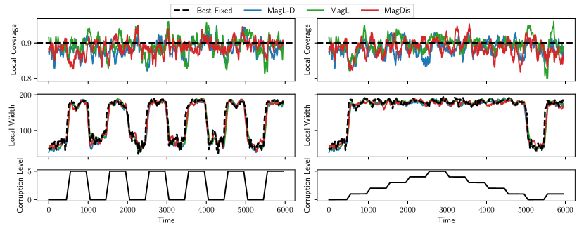
Figure 1: The local coverage (first row), local width (second row), and corresponding corruption level (third row) of our algorithms. Results are obtained using corrupted versions of TinyImageNet, with time-varying corruption level (distribution shift). (Left) Results for sudden changes in corruption level. (Right) Results for gradual changes in corruption level. The distribution shifts every 500 steps. Moving averages are plotted with a window size of 100 time steps ($k=100$).

Figure 1 justifies the validity of our algorithms. Specifically, the local coverage of our algorithms fluctuate around the target coverage of 0.9 for both sudden and gradual distribution shifts. Similarly, the local width approximately replicates the best fixed local width, $\mathrm{Local\,Width}^{*}(t)$, as shown in Figure 1 (middle row).

Hyperparameter sensitivity

We also test the algorithms’ sensitivities to the offline estimate of $D$, which we denote as $D_{\mathrm{est}}$. The baselines Saocp and Sf-Ogd require this parameter to initialize, while Simple OGD and all three of our algorithms do not. To this end, we rerun the experiments above and change the ratio of $D_{\mathrm{est}}$ to the true value $D$. The following settings are tested:

$$\frac{D_{\mathrm{est}}}{D}=\begin{Bmatrix}10^{-3},&10^{-2},&10^{-1},&10^{0},&10^{1},&10^{2},&10^{3}\end{Bmatrix}.$$

We plot the influence of $D_{\mathrm{est}}$ on the average coverage and the average width in Figure 2. For these experiments, we use the case when image corruptions are sudden. Coverage being much larger or much less than 0.9 is not a desirable behavior; given satisfactory coverage, lower width is desirable.

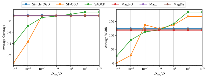
(a)

Figure 2: The average coverage (first row) and average width (second row) as a function of the estimated maximum radius, $D_{\mathrm{est}}$ relative to the true radius $D$. The performance of Sf-Ogd and Saocp [10] are sensitive to $D_{\mathrm{est}}/D$. Averages are taken over the entire time horizon, where the total time steps $T=6011$.

As $D_{\mathrm{est}}/D$ increases, both the average coverage and average width increase for Saocp and Sf-Ogd. In the opposite direction, the average coverage and average width also decrease as $D_{\mathrm{est}}/D$ decrease for Saocp and Sf-Ogd. When $D_{\mathrm{est}}=D$, Simple OGD and Sf-Ogd have approximately equivalent performance. This is not to say that using an offline estimate of $D_{\mathrm{est}}/D$ does not improve performance. The catch is that, for the particular experimental dataset, setting the learning rate to 1 in Simple OGD coincidentally just happens to be a well-picked learning rate, given the true value of the maximum radius magnitude $D$. In contrast, our magnitude learners remain fixed under variations in $D_{\mathrm{est}}/D$, since they do not need $D_{\mathrm{est}}$ to initialize. The baselines SCP, NExCP, Faci, and Faci-S are not presented in Figure 2 as to better highlight the performance of Saocp, OGD, and our magnitude learners. Benchmarks on these additional baselines can be found in [10].

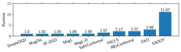
Figure 3: The runtime per time step of each algorithm, normalized to the runtime of Simple OGD. The runtime of Saocp is longest due to it being a meta-algorithm that initializes Sf-Ogd on each time step.

Runtime

We also measure the time for each algorithm to complete a single prediction. Runtime results are provided in Figure 3. The results are normalized relative to the runtime of Simple OGD. Note the runtime standard deviations in Table 1. Accounting for standard deviations, the runtime differences between Simple OGD, Sf-Ogd, MagL, and MagDis are negligible. The runtime of Saocp is longest due to it being a meta-algorithm that initializes Sf-Ogd on each time step, c.f., Appendix A.

References

• AB [23] Anastasios N Angelopoulos and Stephen Bates. Conformal prediction: A gentle introduction. Foundations and Trends® in Machine Learning, 16(4):494–591, 2023.
• ABVR+ [23] David Abel, André Barreto, Benjamin Van Roy, Doina Precup, Hado van Hasselt, and Satinder Singh. A definition of continual reinforcement learning. arXiv preprint arXiv:2307.11046, 2023.
• AKCV [16] Dmitry Adamskiy, Wouter M Koolen, Alexey Chernov, and Vladimir Vovk. A closer look at adaptive regret. Journal of Machine Learning Research, 17(1):706–726, 2016.
• AZKD [24] Kwangjun Ahn, Zhiyu Zhang, Yunbum Kook, and Yan Dai. Understanding Adam optimizer via online learning of updates: Adam is FTRL in disguise. arXiv preprint arXiv:2402.01567, 2024.
• BCRT [23] Rina Foygel Barber, Emmanuel J Candes, Aaditya Ramdas, and Ryan J Tibshirani. Conformal prediction beyond exchangeability. The Annals of Statistics, 51(2):816–845, 2023.
• BGJ+ [22] Osbert Bastani, Varun Gupta, Christopher Jung, Georgy Noarov, Ramya Ramalingam, and Aaron Roth. Practical adversarial multivalid conformal prediction. Advances in Neural Information Processing Systems, 35:29362–29373, 2022.
• BS [19] Noam Brown and Tuomas Sandholm. Solving imperfect-information games via discounted regret minimization. In Proceedings of the AAAI Conference on Artificial Intelligence, volume 33, pages 1829–1836, 2019.
• BW [21] Dheeraj Baby and Yu-Xiang Wang. Optimal dynamic regret in exp-concave online learning. In Conference on Learning Theory, pages 359–409. PMLR, 2021.
• BW [22] Dheeraj Baby and Yu-Xiang Wang. Optimal dynamic regret in proper online learning with strongly convex losses and beyond. In International Conference on Artificial Intelligence and Statistics, pages 1805–1845. PMLR, 2022.
• BWXB [23] Aadyot Bhatnagar, Huan Wang, Caiming Xiong, and Yu Bai. Improved online conformal prediction via strongly adaptive online learning. In International Conference on Machine Learning, pages 2337–2363. PMLR, 2023.
• CBGLS [12] Nicolo Cesa-Bianchi, Pierre Gaillard, Gábor Lugosi, and Gilles Stoltz. Mirror descent meets fixed share (and feels no regret). Advances in Neural Information Processing Systems, 25, 2012.
• CBL [06] Nicolo Cesa-Bianchi and Gábor Lugosi. Prediction, learning, and games. Cambridge university press, 2006.
• CLW [21] Liyu Chen, Haipeng Luo, and Chen-Yu Wei. Impossible tuning made possible: A new expert algorithm and its applications. In Conference on Learning Theory, pages 1216–1259. PMLR, 2021.
• CMO [23] Ashok Cutkosky, Harsh Mehta, and Francesco Orabona. Optimal, stochastic, non-smooth, non-convex optimization through online-to-non-convex conversion. In International Conference on Machine Learning, pages 6643–6670. PMLR, 2023.
• CO [18] Ashok Cutkosky and Francesco Orabona. Black-box reductions for parameter-free online learning in banach spaces. In Conference On Learning Theory, pages 1493–1529. PMLR, 2018.
• Cut [18] Ashok Cutkosky. Algorithms and Lower Bounds for Parameter-free Online Learning. Stanford University, 2018.
• Cut [19] Ashok Cutkosky. Artificial constraints and hints for unbounded online learning. In Conference on Learning Theory, pages 874–894. PMLR, 2019.
• Cut [20] Ashok Cutkosky. Parameter-free, dynamic, and strongly-adaptive online learning. In International Conference on Machine Learning, pages 2250–2259. PMLR, 2020.
• CZ [10] Alexey Chernov and Fedor Zhdanov. Prediction with expert advice under discounted loss. In International Conference on Algorithmic Learning Theory, pages 255–269. Springer, 2010.
• DGIM [02] Mayur Datar, Aristides Gionis, Piotr Indyk, and Rajeev Motwani. Maintaining stream statistics over sliding windows. SIAM journal on computing, 31(6):1794–1813, 2002.
• DGSS [15] Amit Daniely, Alon Gonen, and Shai Shalev-Shwartz. Strongly adaptive online learning. In International Conference on Machine Learning, pages 1405–1411. PMLR, 2015.
• DHS [11] John Duchi, Elad Hazan, and Yoram Singer. Adaptive subgradient methods for online learning and stochastic optimization. Journal of Machine Learning Research, 12(7), 2011.
• DK [20] Nadejda Drenska and Robert V Kohn. Prediction with expert advice: A PDE perspective. Journal of Nonlinear Science, 30(1):137–173, 2020.
• FH [08] Yoav Freund and Daniel Hsu. A new hedging algorithm and its application to inferring latent random variables. arXiv preprint arXiv:0806.4802, 2008.
• FHPF [22] Huang Fang, Nicholas JA Harvey, Victor S Portella, and Michael P Friedlander. Online mirror descent and dual averaging: keeping pace in the dynamic case. Journal of Machine Learning Research, 23(1):5271–5308, 2022.
• FKMS [17] Dylan J Foster, Satyen Kale, Mehryar Mohri, and Karthik Sridharan. Parameter-free online learning via model selection. Advances in Neural Information Processing Systems, 30, 2017.
• GC [21] Isaac Gibbs and Emmanuel Candes. Adaptive conformal inference under distribution shift. Advances in Neural Information Processing Systems, 34:1660–1672, 2021.
• GC [22] Isaac Gibbs and Emmanuel Candès. Conformal inference for online prediction with arbitrary distribution shifts. arXiv preprint arXiv:2208.08401, 2022.
• Haa [81] Uffe Haagerup. The best constants in the khintchine inequality. Studia Mathematica, 70(3):231–283, 1981.
• Haz [22] Elad Hazan. Introduction to online convex optimization. MIT Press, 2022.
• HLPR [23] Nicholas JA Harvey, Christopher Liaw, Edwin Perkins, and Sikander Randhawa. Optimal anytime regret with two experts. Mathematical Statistics and Learning, 6(1):87–142, 2023.
• HS [09] Elad Hazan and Comandur Seshadhri. Efficient learning algorithms for changing environments. In International Conference on Machine Learning, pages 393–400, 2009.
• IHC [23] Maor Ivgi, Oliver Hinder, and Yair Carmon. Dog is SGD’s best friend: A parameter-free dynamic step size schedule. In International Conference on Machine Learning, pages 14465–14499. PMLR, 2023.
• JC [22] Andrew Jacobsen and Ashok Cutkosky. Parameter-free mirror descent. In Conference on Learning Theory, pages 4160–4211. PMLR, 2022.
• JOWW [17] Kwang-Sung Jun, Francesco Orabona, Stephen Wright, and Rebecca Willett. Improved strongly adaptive online learning using coin betting. In Artificial Intelligence and Statistics, pages 943–951. PMLR, 2017.
• KB [14] Diederik P Kingma and Jimmy Ba. Adam: A method for stochastic optimization. arXiv preprint arXiv:1412.6980, 2014.
• KP [11] Michael Kapralov and Rina Panigrahy. Prediction strategies without loss. Advances in Neural Information Processing Systems, 24, 2011.
• KW [52] Jack Kiefer and Jacob Wolfowitz. Stochastic estimation of the maximum of a regression function. The Annals of Mathematical Statistics, pages 462–466, 1952.
• LH [23] Zhou Lu and Elad Hazan. On the computational efficiency of adaptive and dynamic regret minimization. arXiv preprint arXiv:2207.00646, 2023.
• McM [17] H Brendan McMahan. A survey of algorithms and analysis for adaptive online learning. Journal of Machine Learning Research, 18(1):3117–3166, 2017.
• MK [20] Zakaria Mhammedi and Wouter M Koolen. Lipschitz and comparator-norm adaptivity in online learning. In Conference on Learning Theory, pages 2858–2887. PMLR, 2020.
• MO [14] H Brendan McMahan and Francesco Orabona. Unconstrained online linear learning in hilbert spaces: Minimax algorithms and normal approximations. In Conference on Learning Theory, pages 1020–1039. PMLR, 2014.
• OP [16] Francesco Orabona and Dávid Pál. Coin betting and parameter-free online learning. Advances in Neural Information Processing Systems, 29, 2016.
• OP [18] Francesco Orabona and Dávid Pál. Scale-free online learning. Theoretical Computer Science, 716:50–69, 2018.
• OP [21] Francesco Orabona and Dávid Pál. Parameter-free stochastic optimization of variationally coherent functions. arXiv preprint arXiv:2102.00236, 2021.
• Opp [99] Alan V Oppenheim. Discrete-time signal processing. Pearson Education, 1999.
• [47] Francesco Orabona. A modern introduction to online learning. arXiv preprint arXiv:1912.13213, 2023.
• [48] Francesco Orabona. Normalized gradients for all. arXiv preprint arXiv:2308.05621, 2023.
• RM [51] Herbert Robbins and Sutton Monro. A stochastic approximation method. The annals of mathematical statistics, pages 400–407, 1951.
• Rot [22] Aaron Roth. Uncertain: Modern topics in uncertainty estimation, 2022.
• SM [12] Matthew Streeter and Brendan Mcmahan. No-regret algorithms for unconstrained online convex optimization. Advances in Neural Information Processing Systems, 25, 2012.
• TH+ [12] Tijmen Tieleman, Geoffrey Hinton, et al. Lecture 6.5-rmsprop: Divide the gradient by a running average of its recent magnitude. COURSERA: Neural networks for machine learning, 4(2):26–31, 2012.
• VGS [05] Vladimir Vovk, Alexander Gammerman, and Glenn Shafer. Algorithmic learning in a random world, volume 29. Springer, 2005.
• ZCP [22] Zhiyu Zhang, Ashok Cutkosky, and Ioannis Paschalidis. PDE-based optimal strategy for unconstrained online learning. In International Conference on Machine Learning, pages 26085–26115. PMLR, 2022.
• ZCP [23] Zhiyu Zhang, Ashok Cutkosky, and Ioannis Ch Paschalidis. Unconstrained dynamic regret via sparse coding. arXiv preprint arXiv:2301.13349, 2023.
• ZFG+ [22] Margaux Zaffran, Olivier Féron, Yannig Goude, Julie Josse, and Aymeric Dieuleveut. Adaptive conformal predictions for time series. In International Conference on Machine Learning, pages 25834–25866. PMLR, 2022.
• Zin [03] Martin Zinkevich. Online convex programming and generalized infinitesimal gradient ascent. In International Conference on Machine Learning, pages 928–936, 2003.
• ZLZ [18] Lijun Zhang, Shiyin Lu, and Zhi-Hua Zhou. Adaptive online learning in dynamic environments. Advances in neural information processing systems, 31, 2018.
• ZYCP [23] Zhiyu Zhang, Heng Yang, Ashok Cutkosky, and Ioannis Ch Paschalidis. Improving adaptive online learning using refined discretization. arXiv preprint arXiv:2309.16044, 2023.
• ZYZ [18] Lijun Zhang, Tianbao Yang, and Zhi-Hua Zhou. Dynamic regret of strongly adaptive methods. In International Conference on Machine Learning, pages 5882–5891. PMLR, 2018.
• ZZZZ [20] Peng Zhao, Yu-Jie Zhang, Lijun Zhang, and Zhi-Hua Zhou. Dynamic regret of convex and smooth functions. Advances in Neural Information Processing Systems, 33:12510–12520, 2020.