Entangling two exciton modes using exciton optomechanics

Abstract

Exciton optomechanics, bridging cavity exciton polaritons and optomechanics, opens new opportunities for the study of light-matter strong interactions and nonlinearities, due to the rich nonlinear couplings among excitons, phonons, and photons. Here, we propose to entangle two exciton modes in an exciton-optomechanical system, which consists of a semiconductor optomechanical microcavity integrated with two quantum wells. The quantum wells support two exciton modes, which simultaneously couple to an optical cavity mode via a linear coupling, and the cavity mode also couples to a mechanical vibration mode via a dispersive optomechanical interaction, accounting for both the radiation pressure and the photoelastic effect. We show that by strongly driving the microcavity with a red-detuned laser field and when the two exciton modes are respectively resonant with the Stokes and anti-Stokes sidebands scattered by the mechanical motion, stationary entanglement between the two exciton modes can be established under currently available parameters. The entanglement is robust against various dissipations of the system and can be achieved at room temperature for a mechanical quality factor higher than $\sim 10^{4}$.

I Introduction

Semiconductor optomechanical microcavities integrated with quantum wells (QWs) can simultaneously confine photons, phonons and excitons in a compact mode volume and achieve strong coupling among them review ; EOM1 ; EOM2 ; EOM3 . This novel hybrid system is termed as exciton optomechanics review . The strong coupling between excitons and microcavity photons leads to exciton polaritons Hopfield58 ; Weisbuch92 , a type of half-matter half-light bosons with a very small effective mass Keeling07 ; Deng10 . In the past decades, significant progress has been made in exciton polaritons in both fundamental physics and practical applications, e.g., Bose-Einstein condensation BEC1 ; BEC2 , light emitting diodes Tsintzos08 , and low-threshold room-temperature polariton lasers Imamoglu96 ; Christopoulos07 ; Kena-Cohen10 have been achieved.

The dual light-matter nature of exciton polaritons also leads to a tunable and strongly enhanced polariton-mechanics coupling Barg18 ; Kobecki22 , because the exciton-phonon interaction can be much stronger Bir ; EOM3 than the two types of the optomechanical interaction, i.e., radiation pressure MA14 and photoelasticity Perrin13 ; Favero14 . A near-unity single-polariton quantum cooperativity is promising to be achieved using current semiconductor resonator platforms EOM3 . Moreover, in such a semiconductor configuration, exciton polaritons can be efficiently pumped by the electrical current, which offers an additional effective means to control the system dynamics Schneider13 ; Bhattacharya13 ; Bhattacharya14 , and the exciton component can bring in rich nonlinearities to the system, including the exciton-exciton and -phonon interactions. Meanwhile, highly monochromatic phonons at gigahertz can be generated by bulk acoustic wave resonators and effectively injected into the microcavity to modulate the polaritonic states Santos21 . Coherent mechanical self-oscillation can be achieved via the polariton drive and the phonon laser Fainstein20 and the microwave-optical conversion Santos23 have been realized in this hybrid system.

Exciton optomechanics exhibits a wealth of unexplored physics and prospective applications that can be uncovered by combining quantum optics and semiconductor physics. However, so far research in this field has predominantly focused on the classical phenomena, and the quantum effects have been rarely explored review ; EOM3 . Here, we present a quantum theory for achieving stationary entanglement of two exciton modes by exploiting the dispersive optomechanical interaction in an exciton-optomechanical system, which contains two QWs supporting two exciton modes. Specifically, a strong red-detuned laser is used to drive the microcavity, which effectively cools the mechanical mode by activating the optomechanical anti-Stokes scattering. The Stokes scattering is also activated by keeping one of the exciton modes resonant with the Stokes sideband, which creates entanglement. When the other exciton mode is further resonant with the anti-Stokes sideband, the two exciton modes become entangled. The entanglement is in the steady state and robust against various dissipations of the system and bath temperature, and can survive even at room temperature for a mechanical quality factor reaching about $10^{4}$.

The paper is organized as follows. In Sec. II, we introduce the exciton-optomechanical system involving an optomechanical cavity and two exciton modes, and provide its Hamiltonian and the corresponding quantum Langevin equations (QLEs). We further show how to linearize the dynamics and achieve the steady-state entanglement of the two exciton modes. In Sec. III, we present the results of the exciton-exciton entanglement and analyze the impact of the couplings and dissipations of the system on the entanglement. In particular, we provide the conditions under which room-temperature exciton entanglement can be achieved. Finally, we conclude in Sec. IV .

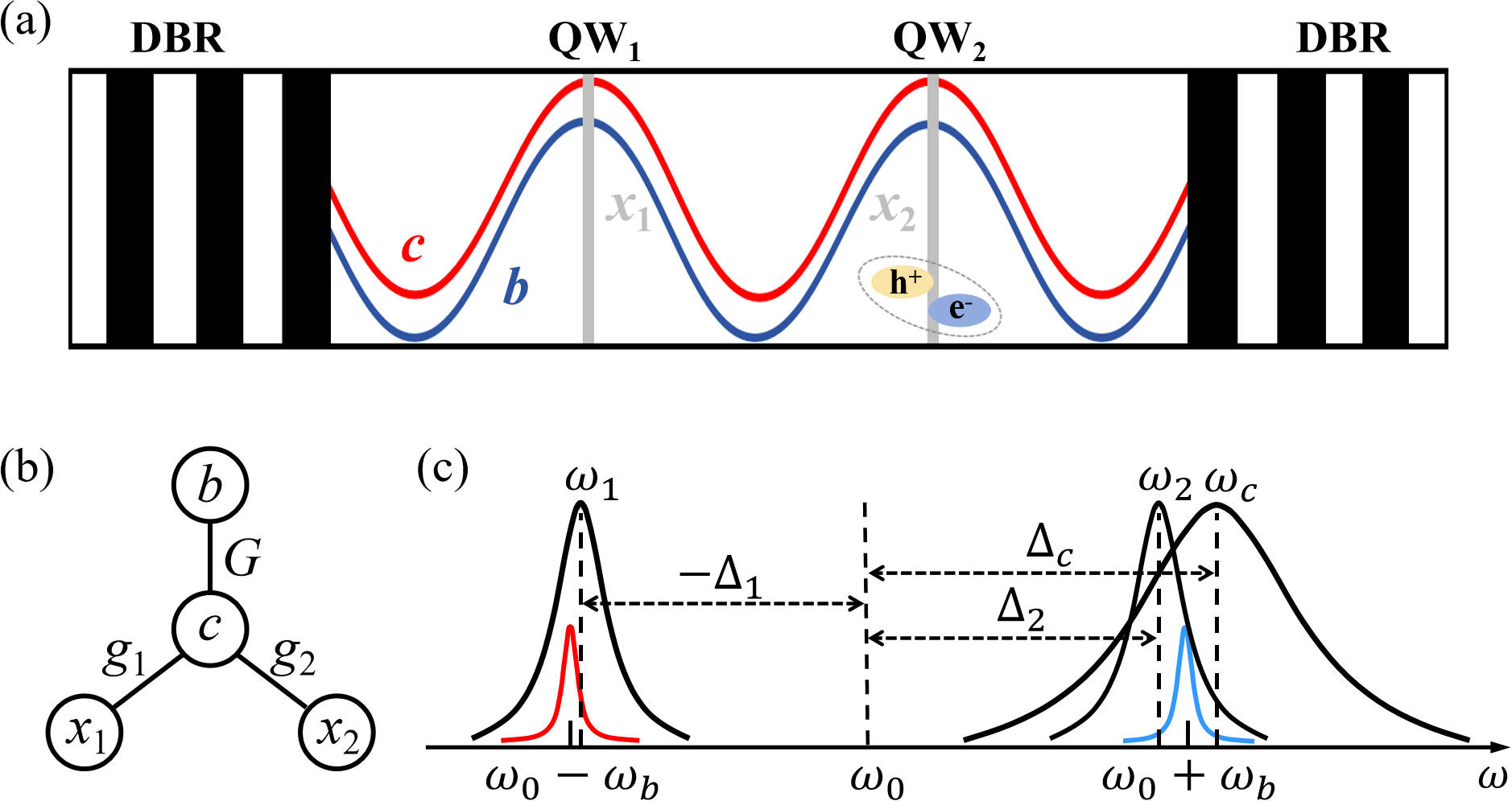
Figure 1: (a) Sketch of the exciton-optomechanical system. A semiconductor microcavity formed by two movable DBRs establishes an optomechanical interaction between the cavity mode $c$ and the mechanical mode $b$. Two QWs are placed at the antinodes of the cavity field, confining two exciton modes $x_{1}$ and $x_{2}$. (b) The cavity mode $c$ couples to the two exciton modes $x_{1}$ and $x_{2}$ via a linear beam-splitter interaction and to the mechanical mode $b$ via a dispersive interaction. (c) The semiconductor microcavity is strongly driven by a laser at frequency $\omega_{0}$, and the mechanical motion of frequency $\omega_{b}$ scatters the driving photons onto two sidebands at $\omega_{0}\pm\omega_{b}$. When the cavity mode with frequency $\omega_{c}$ is resonant with the anti-Stokes sideband and the two exciton modes with frequencies $\omega_{1,2}$ are respectively resonant with the two mechanical sidebands, the two exciton modes get entangled.

II The model

We consider a hybrid exciton-optomechanical system EOM1 ; EOM2 ; EOM3 , which consists of a semiconductor microcavity sandwiched between two distributed Bragg reflectors (DBRs) and two QWs that are placed at two antinodes of the cavity field, as depicted in Fig. 1(a). The DBRs are constructed from layers with alternating high and low refractive indices and act as high-reflectivity mirrors to effectively confine optical photons. Due to the radiation-pressure and the photoelastic interaction, the microcavity layer and DBRs vibrate, promising a dispersive optomechanical coupling of the cavity mode with the vibration phonon mode Perrin13 ; Favero14 . Each QW supports an exciton mode, where electrons and holes form dipoles capable of interacting with an electromagnetic field, embodied by a linear beam-splitter-type exciton-photon interaction. Since the QWs are positioned at the maxima of the confined electromagnetic field, corresponding to the maximum mechanical displacement and thus vanishing phonon strain at the QW positions Perrin13 , the coupling between excitons and phonons is negligible review . Therefore, the Hamiltonian of such a quadripartite system, cf. Fig. 1(b), reads

$$\begin{split}H/\hbar&=\!\omega_{1}x_{1}^{\dagger}x_{1}+\omega_{2}x_{2}^{\dagger}x_{2}+\omega_{c}c^{\dagger}c+\omega_{b}b^{\dagger}b+G_{0}c^{\dagger}c\left(b+b^{\dagger}\right)\\ &+\sum_{k=1,2}g_{k}\left(x_{k}^{\dagger}c+x_{k}c^{\dagger}\right)+i\Omega\left(c^{\dagger}e^{-i\omega_{0}t}-ce^{i\omega_{0}t}\right),\end{split}$$ (1)

where $x_{1}$, $x_{2}$, $c$ and $b$ ($x_{1}^{\dagger}$, $x_{2}^{\dagger}$, $c^{\dagger}$ and $b^{\dagger}$) are the annihilation (creation) operators of the two exciton modes, the cavity mode, and the mechanical mode, respectively, satisfying $[j,j^{\dagger}]=1$ ($j=x_{1},\,x_{2},\,c,\,b$), and $\omega_{1}$, $\omega_{2}$, $\omega_{c}$, and $\omega_{b}$ are their corresponding resonance frequencies. The bare coupling strength $G_{0}$ includes both the optomechanical interactions associated with the radiation pressure and the photoelastic effect EOM3 ; Favero14 , which are both dispersive couplings; $g_{1}$ and $g_{2}$ denote the coupling strengths between the cavity mode with the two exciton modes, which can be much stronger than the cavity decay rate $\kappa_{c}$ and the exciton dissipation rates $\kappa_{1},\,\kappa_{2}$, resulting in the formation of exciton polaritons Hopfield58 ; Weisbuch92 . The last term corresponds to the driving Hamiltonian, and $\Omega=\sqrt{2P\kappa_{c}/\hbar\omega_{0}}$ denotes the coupling strength between the drive field and the microcavity, with $\omega_{0}$ and $P$ being the frequency and power of the driving laser.

Including the dissipations and input noises of the system, we obtain the following QLEs in the frame rotating at the drive frequency $\omega_{0}$:

$$\begin{split}\dot{x}_{1}=&-(i\Delta_{1}+\kappa_{1})x_{1}-ig_{1}c+\sqrt[]{2\kappa_{1}}x_{1}^{in},\\ \dot{x}_{2}=&-(i\Delta_{2}+\kappa_{2})x_{2}-ig_{2}c+\sqrt[]{2\kappa_{2}}x_{2}^{in},\\ \dot{c}=&-(i\Delta_{c}+\kappa_{c})c-i\!\sum_{k=1,2}g_{k}x_{k}-iG_{0}c(b+b^{\dagger})+\Omega+\sqrt[]{2\kappa_{c}}c^{in},\\ \dot{b}=&-(i\omega_{b}+\kappa_{b})b-iG_{0}c^{\dagger}c+\sqrt[]{2\kappa_{b}}b^{in},\end{split}$$ (2)

where $\Delta_{k}=\omega_{k}-\omega_{0}$ ($k=1,2$) and $\Delta_{c}=\omega_{c}-\omega_{0}$; $\kappa_{b}$ is the mechanical damping rate, and $j^{in}(t)$ are the input noise operators for the mode $j$ ($j=x_{1},\,x_{2},\,c,\,b$), which are zero mean and characterized by the correlation functions Zoller : $\langle j^{in}(t)j^{in\dagger}(t^{\prime})\rangle=[N_{j}(\omega_{j})+1]\delta(t-t^{\prime})$, $\langle j^{in\dagger}(t)j^{in}(t^{\prime})\rangle=N_{j}(\omega_{j})\delta(t-t^{\prime})$, with $N_{j}(\omega_{j})=[\exp[(\hbar\omega_{j}/k_{B}T)]-1]^{-1}$ being the equilibrium mean thermal excitation number of the mode $j$, and $k_{B}$ as the Boltzmann constant and $T$ the bath temperature.

The cavity is strongly driven by an intense laser field to enhance the dispersive optomechanical coupling, leading to a large amplitude of the cavity field $|\langle c\rangle|\gg 1$. This allows us to linearize the system dynamics around the large average values by writing each mode operator $j$ as its average $\langle j\rangle$ plus the quantum fluctuation operator $\delta j$, i.e., $j=\langle j\rangle\,+\,\delta j$, and neglecting small second-order fluctuation terms. Consequently, we obtain two sets of equations for the classical averages and the quantum fluctuations, respectively. The former set of equations are given by

$$\begin{split}\langle x_{1}\rangle=&\frac{-ig_{1}\langle c\rangle}{i{\Delta}_{1}+\kappa_{1}},\,\,\,\,\,\,\,\,\,\langle x_{2}\rangle=\frac{-ig_{2}\langle c\rangle}{i{\Delta}_{2}+\kappa_{2}},\\ \langle c\rangle=&\frac{\Omega(i{\Delta}_{1}+\kappa_{1})(i{\Delta}_{2}+\kappa_{2})}{g_{1}^{2}(i{\Delta}_{2}{+}\kappa_{2})\,{+}g_{2}^{2}(i{\Delta}_{1}{+}\kappa_{1})\,{+}\,(i\tilde{\Delta}_{c}{+}\kappa_{c})(i{\Delta}_{1}{+}\kappa_{1})(i{\Delta}_{2}{+}\kappa_{2})},\\ \langle b\rangle=&-\frac{G_{0}}{{\omega_{b}}}|\langle c\rangle|^{2},\end{split}$$ (3)

where $\tilde{\Delta}_{c}={\Delta}_{c}+2G_{0}\langle b\rangle$ is the effective cavity-drive detuning, including the frequency shift caused by the optomechanical interaction. The linearized QLEs for the quantum fluctuations are

$$\begin{split}\dot{\delta x}_{1}=&-\big{(}i{\Delta}_{1}+\kappa_{1}\big{)}\delta x_{1}-ig_{1}{\delta c}+\sqrt[]{2\kappa_{1}}x_{1}^{in},\\ \dot{\delta x}_{2}=&-\big{(}i{\Delta}_{2}+\kappa_{2}\big{)}\delta x_{2}-ig_{2}{\delta c}+\sqrt[]{2\kappa_{2}}x_{2}^{in},\\ \dot{\delta c}=&-\big{(}i\tilde{\Delta}_{c}+\kappa_{c}\big{)}\delta c-i\!\sum_{k=1,2}g_{k}{\delta x}_{k}-G\big{(}\delta b+\delta b^{\dagger}\big{)}+\sqrt[]{2\kappa_{c}}c^{in},\\ \dot{\delta b}=&-\big{(}i{\omega}_{b}+\kappa_{b}\big{)}\delta b-\big{(}G\delta c^{\dagger}-G^{*}\delta c\big{)}+\sqrt[]{2\kappa_{b}}b^{in},\end{split}$$ (4)

with $G=iG_{0}\langle c\rangle$ being the effective optomechanical coupling strength, which is generally complex.

The above QLEs (4) can be expressed in a concise matrix form in terms of the quadrature fluctuations $\delta X_{j}=(\delta j+\delta j^{\dagger})/\!\sqrt{2}$, $\delta Y_{j}=i(\delta j^{\dagger}-\delta j)/\!\sqrt{2}$ and the quadrature form of the input noises $X_{j}^{in}$ and $Y_{j}^{in}$ defined analogously, i.e.,

$$\dot{u}(t)=A\,u(t)+n(t),$$ (5)

where $u(t)=[\delta X_{x_{1}}(t),\delta Y_{x_{1}}(t),\delta X_{x_{2}}(t),\delta Y_{x_{2}}(t),\delta X_{c}(t),\delta Y_{c}(t)$, $\delta X_{b}(t),\delta Y_{b}(t)]^{\rm T}$, $n(t)=[\sqrt[]{2\kappa_{1}}X_{x_{1}}^{in},\sqrt[]{2\kappa_{1}}Y_{x_{1}}^{in},\sqrt[]{2\kappa_{2}}X_{x_{2}}^{in},\sqrt[]{2\kappa_{2}}Y_{x_{2}}^{in}$, $\sqrt[]{2\kappa_{c}}X_{c}^{in},\sqrt[]{2\kappa_{c}}Y_{c}^{in},\sqrt[]{2\kappa_{b}}X_{b}^{in},\sqrt[]{2\kappa_{b}}Y_{b}^{in}]^{\rm T}$, and the drift matrix $A$ is given by

$$A=\begin{pmatrix}-\kappa_{1}&{\Delta}_{1}&0&0&0&g_{1}&0&0\\ -{\Delta}_{1}&-\kappa_{1}&0&0&-g_{1}&0&0&0\\ 0&0&-\kappa_{2}&{\Delta}_{2}&0&g_{2}&0&0\\ 0&0&-{\Delta}_{2}&-\kappa_{2}&-g_{2}&0&0&0\\ 0&g_{1}&0&g_{2}&-\kappa_{c}&\tilde{\Delta}_{c}&-2{\rm Re}\,G&0\\ -g_{1}&0&-g_{2}&0&-\tilde{\Delta}_{c}&-\kappa_{c}&-2{\rm Im}\,G&0\\ 0&0&0&0&0&0&-\kappa_{b}&\omega_{b}\\ 0&0&0&0&-2{\rm Im}\,G&2{\rm Re}\,G&-\omega_{b}&-\kappa_{b}\\ \end{pmatrix}.$$ (6)

Because the quantum noises are Gaussian and the system dynamics is linearized, the steady state of the quantum fluctuations is a continuous variable four-mode Gaussian state, which can be completely characterized by an $8\times 8$ covariance matrix (CM) $\cal V$, with the entries ${\cal V}_{ij}=\frac{1}{2}\langle u_{i}(t)u_{j}(t^{\prime})+u_{j}(t^{\prime})u_{i}(t)\rangle$ $(i,j=1,2,...,8)$, as the first moments of the quadrature fluctuations are zero. The steady-state CM can be straightforwardly achieved by solving the Lyapunov equation Vitali07 ; Parks .

$$\begin{split}A{\cal V}+{\cal V}A^{\rm T}=-D,\end{split}$$ (7)

where $D=\mathrm{Diag}\big{[}\kappa_{1}(2N_{x_{1}}{+}1),\kappa_{1}(2N_{x_{1}}{+}1),\kappa_{2}(2N_{x_{2}}{+}1),\kappa_{2}(2N_{x_{2}}$ $+1),\kappa_{c}(2N_{c}{+}1),\kappa_{c}(2N_{c}{+}1),\kappa_{b}(2N_{b}{+}1),\kappa_{b}(2N_{b}{+}1)\big{]}$ is the diffusion matrix, which is defined by $\langle n_{i}(t)n_{j}(t^{\prime})+n_{j}(t^{\prime})n_{i}(t)\rangle/2=D_{ij}\,\delta(t-t^{\prime})$. With the CM in hand, the entanglement of two exciton modes can then be quantified by calculating the logarithmic negativity Ent , which for Gaussian states is defined as

$$\begin{split}E_{N}\equiv\max[0,-\ln 2\tilde{\nu}_{-}],\end{split}$$ (8)

where $\tilde{\nu}_{-}=\min{\rm eig}|i\Omega_{2}\tilde{{\cal V}}_{\rm ex}|$ (the symplectic matrix $\Omega_{2}=\oplus_{j=1}^{2}i\sigma_{y}$ and $\sigma_{y}$ is the $y$-Pauli matrix) is the minimum symplectic eigenvalue of the CM $\tilde{{\cal V}}_{\rm ex}={\cal P}{\cal V}_{\rm ex}{\cal P}$, with ${\cal V}_{\rm ex}$ being the $4\times 4$ CM of the two exciton modes obtained by removing in $\cal V$ the rows and columns associated with the cavity and mechanical modes, and ${\cal P}=\mathrm{Diag}[1,-1,1,1]$ being the matrix that performs partial transposition on the CM.

III Exciton-exciton entanglement

In typical semiconductor optomechanical microcavities EOM1 ; EOM3 ; Perrin13 , the mechanical frequency is high and in the gigahertz range. Although the mean thermal occupation of the mechanical mode is small at low bath temperatures, it becomes large at high temperatures, which inhibits the generation of quantum states at, e.g., room temperature. To eliminate this dominant thermal noise of the system, we use a red-detuned laser to drive the microcavity with the detuning $\tilde{\Delta}_{c}\approx\omega_{b}$ (Fig. 1(c)), which activates the optomechanical anti-Stokes scattering and realizes the mechanical cooling interaction. Further, the driving power should be sufficiently strong to yield a sufficiently strong optomechanical effective coupling $G$, such that the weak coupling condition $|G|\ll\omega_{b}$ for taking the rotating-wave approximation is broken, and consequently, the counter-rotating-wave terms, $\propto\delta{c}^{\dagger}\delta{b}^{\dagger}+\delta{c}\delta{b}$, play the role in creating the optomechanical entanglement Vitali07 ; Vitali08 . This corresponds to the generation of the Stokes sideband associated with the parameter down conversion (PDC) process. A similar mechanism is adopted to produce the magnomechanical entanglement Li18 .

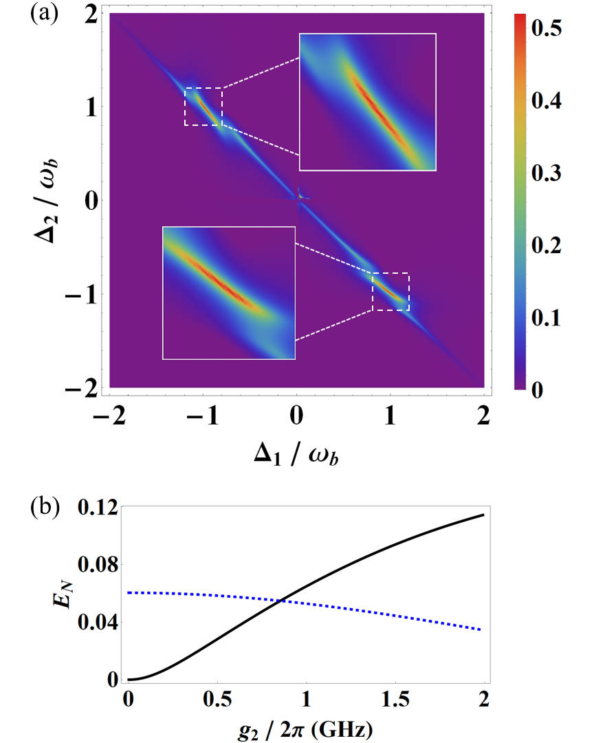
Figure 2: (a) Density plot of the stationary entanglement between two exciton modes versus two exciton-drive detunings $\Delta_{1}$ and $\Delta_{2}$. Insets: zoom-in of the optimal detuning regimes. (b) Stationary exciton-exciton entanglement $E_{x_{1},x_{2}}$ (solid) and cavity-exciton ($x_{1}$) entanglement $E_{c,x_{1}}$ (dashed) versus the exciton-photon coupling $g_{2}$. We take $\tilde{\Delta}_{c}=0.9\omega_{b}$ in (a) and (b), and $\Delta_{1}=-0.95\omega_{b}$ and $\Delta_{2}=\omega_{b}$ in (b). The other parameters are provided in the text.

We find that when the two exciton modes are resonant with the Stokes and anti-Stokes sidebands, respectively, they get entangled, as shown in Fig. 2(a). In the Stokes process, the Stokes photons and the phonons are entangled because of the PDC; while in the anti-Stokes process, the anti-Stokes photons and the phonons realize an effective state-swap interaction. Therefore, due to the mediation of the phonons in these two processes, the Stokes and anti-Stokes sidebands become entangled. Since the excitons and cavity photons also share a beam-splitter (state-swap) interaction, the two exciton modes are thus entangled when they are respectively resonant with the two sidebands. This is reflected by the fact that the exciton-exciton entanglement is maximized at two optimal detuning conditions $\Delta_{1}=-\Delta_{2}=\pm\omega_{b}$ in Fig. 2(a), because the two exciton modes are exchange invariant in our model, cf. Eq. (1). In Fig. 2(b), we show the exciton-exciton entanglement $E_{x_{1},x_{2}}$ and the cavity-exciton ($x_{1}$) entanglement $E_{c,x_{1}}$ as a function of the exciton-photon coupling $g_{2}$. The increasing (declining) entanglement $E_{x_{1},x_{2}}$ ($E_{c,x_{1}}$) with the coupling clearly manifests the key role of the exciton-photon state-swap interaction in distributing the entanglement to the exciton modes. The fact that the increase of $E_{x_{1},x_{2}}$ is greater than the decrease of $E_{c,x_{1}}$ is because the extra entanglement is transferred from other bipartite or multipartite subsystems (not shown). Such an involved entanglement distribution among different subsystems is a typical feature of the entanglement in multipartite systems Li18 ; LPR . In getting Fig. 2, we use experimentally feasible parameters review ; EOM1 ; EOM3 ; Perrin13 : $\omega_{b}/2\pi=20$ GHz, $\kappa_{b}/2\pi=1$ MHz, $\kappa_{c}/2\pi=1$ GHz, $\kappa_{1(2)}/2\pi=10^{2}$ MHz, $g_{1(2)}/2\pi=2$ GHz, $G_{0}/2\pi=10$ MHz, $\Omega/2\pi=6$ THz, and $T=1$ K. Under the optimal detunings in Fig. 2(a), the mechanical motion is cooled into its quantum ground state with an effective mean phonon number of 0.22. This corresponds to the drive power $P\approx 22$ mW for $\omega_{0}/2\pi\approx 3\times 10^{2}$ THz.

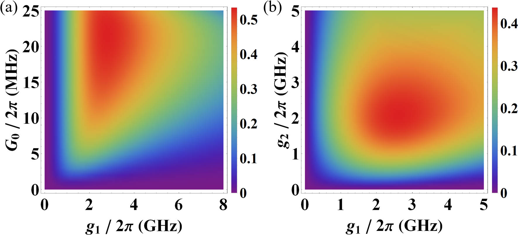
Figure 3: Stationary exciton-exciton entanglement versus (a) exciton-photon coupling $g_{1}$ $(=g_{2})$ and bare optomechanical coupling $G_{0}$; (b) exciton-photon couplings $g_{1}$ and $g_{2}$. We take the optimal detunings $\tilde{\Delta}_{c}=0.9\omega_{b}$ and $\Delta_{1}=-\Delta_{2}=-\omega_{b}$. The other parameters are the same as in Fig. 2.

Figure 3(a) studies the entanglement versus the exciton-photon coupling $g_{1(2)}$ and the bare optomechanical coupling $G_{0}$ (with a fixed drive power). Clearly, it manifests the indispensable role of the dispersive optomechanical coupling in creating the exciton-exciton entanglement: the entanglement is present only for a nonzero $G_{0}\neq 0$, and $G_{0}$ (and thus $G$) should be sufficiently strong to activate the optomechanical PDC interaction, as discussed above, but it cannot be too strong, which leads the system to be unstable. Figure 3(a) shows the results in the steady state, which is guaranteed by the negative eigenvalues (real parts) of the drift matrix $A$. In Fig. 3(b), we plot the entanglement versus the two exciton-photon couplings $g_{1}$ and $g_{2}$. Since the exciton-exciton entanglement is transferred from the entanglement of the two optical sidebands, as analyzed above, a high-efficiency quantum state transfer requires the exciton-photon coupling strength to be greater than the exciton and cavity decay rates, i.e., $g_{1(2)}>\kappa_{1(2)},\kappa_{c}$ Yu20 ; SG21 . Because in typical experiments $\kappa_{c}\gg\kappa_{1(2)}$, the entanglement is maximized in the regime of $g_{1(2)}>\kappa_{c}=2\pi\times 1$ GHz. However, a much larger coupling also reduces the entanglement. This is because it will lead to a considerable exciton-photon normal mode splitting, such that the normal modes, i.e., two exciton polaritons, are no longer resonant with the anti-Stokes sideband (cf. Fig. 1(c)).

In Fig. 4, we study the impact of various dissipation rates and bath temperature on the entanglement. It shows that the entanglement is quite robust against all the dissipation rates of the system: it is present for the cavity (exciton) decay rate being up to $\kappa_{c}/2\pi=10$ GHz ($\kappa_{1(2)}/2\pi=1$ GHz) under the parameters of Fig. 2; see Fig. 4(a), which are within the reach of current technology review ; EOM1 ; EOM3 ; Perrin13 . Due to the high mechanical frequency of the system, the entanglement is achievable even at very high temperatures (Fig. 4(b)), e.g., it is nonzero at room temperature for the mechanical damping rate being smaller than $1$ MHz (i.e., the quality factor $Q>2\times 10^{4}$), which is currently accessible review .

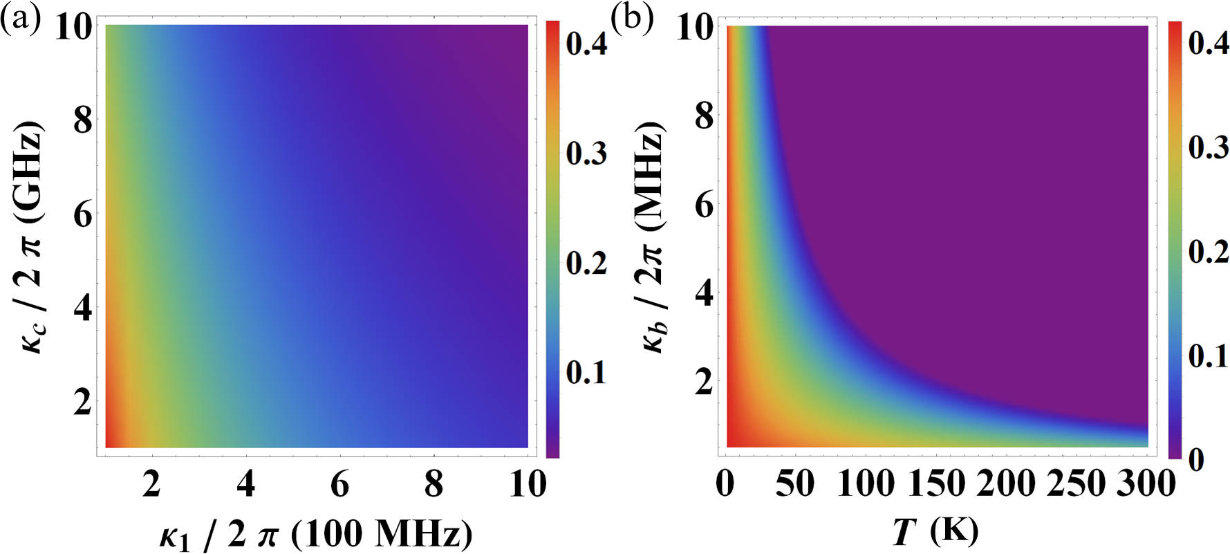
Figure 4: Stationary exciton-exciton entanglement versus (a) exciton and cavity dissipation rates $\kappa_{1}$ $(=\kappa_{2})$ and $\kappa_{c}$; (b) bath temperature $T$ and mechanical damping rate $\kappa_{b}$. We take $\tilde{\Delta}_{c}=0.9\omega_{b}$ and $\Delta_{1}=-\Delta_{2}=-\omega_{b}$. The other parameters are those of Fig. 2.

At last, we show how to detect the generated exciton-exciton entanglement. The entanglement can be verified by measuring the CM of the two exciton modes. This can be realized by sending a weak probe field resonantly driving the cavity. Due to the exciton-photon state-swap interaction, the states of the two exciton modes are then mapped to the output field of the cavity. Therefore, by homodyning the cavity output field one can measure the quadratures of the exciton modes, based on which the CM is reconstructed. It should be noted that the output field carries the states of two exciton modes that differ by twice mechanical frequency in frequency. To measure the quadratures of the exciton mode $x_{1}$, one can send the output field to a filter with the central frequency of $\omega_{1}$, which filters out the other exciton mode. Similarly, one can measure the quadratures of the exciton mode $x_{2}$. This requires that the cavity photons decay much faster than the excitons do (i.e., $\kappa_{c}\gg\kappa_{1,2}$, which is adopted in our proposal), such that when the driving laser is switched off and all cavity photons die out, the exciton states remain almost unchanged, at which time the probe field is sent.

IV Conclusions

We present a theory for entangling two exciton modes in an exciton-optomechanical system, consisting of an optical cavity mode, a mechanical vibration mode, and two exciton modes. The key step is to simultaneously activate both the optomechanical anti-Stokes and Stokes scatterings, responsible for cooling the mechanical motion and creating the optomechanical entanglement, respectively. The Stokes and anti-Stokes sidebands are entangled due to the mediation of the mechanical oscillator in the above two scattering processes. By exploiting the exciton-photon state-swap interaction, the two exciton modes therefore get entangled when they are respectively resonant with the two sidebands. Impressively, room-temperature exciton entanglement can be achieved under currently available parameters in the exciton-optomechanical experiments. The present work enriches the study on quantum effects in the field of exciton optomechanics, and reveals the potential applications of the hybrid system in quantum information science and technology.

References

- (1) P. V. Santos, and A. Fainstein, Polaromechanics: polaritonics meets optomechanics, Opt. Mater. Express 13, 1974 (2023).
- (2) O. Kyriienko, T. C. H. Liew, and I. A. Shelykh, Optomechanics with cavity polaritons: Dissipative coupling and unconventional bistability, Phys. Rev. Lett. 112, 076402 (2014).
- (3) B. Jusserand, A. N. Poddubny, A. V. Poshakinskiy, A. Fainstein, and A. Lemaitre, Polariton resonances for ultrastrong coupling cavity optomechanics in GaAs/AlAs multiple quantum wells, Phys. Rev. Lett. 115, 267402 (2015).
- (4) N. Carlon Zambon, Z. Denis, R. De Oliveira, S. Ravets, C. Ciuti, I. Favero, and J. Bloch, Enhanced cavity optomechanics with quantum-well exciton polaritons, Phys. Rev. Lett. 129, 093603 (2022).
- (5) J. J. Hopfield, Theory of the contribution of excitons to the complex dielectric constant of crystals, Phys. Rev. 112, 1555 (1958).
- (6) C. Weisbuch, M. Nishioka, A. Ishikawa, and Y. Arakawa, Observation of the coupled exciton-photon mode splitting in a semiconductor quantum microcavity, Phys. Rev. Lett. 69, 3314 (1992).
- (7) J Keeling, F M Marchetti, M H Szymańska, and P B Littlewood, Collective coherence in planar semiconductor microcavities, Semicond. Sci. Technol. 22, R1 (2007).
- (8) H. Deng, H. Haug, and Y. Yamamoto, Exciton-polariton Bose-Einstein condensation, Rev. Mod. Phys. 82, 1489 (2010).
- (9) J. Kasprzak, M. Richard, S. Kundermann, A. Baas, P. Jeambrun, J. M. J. Keeling, F. M. Marchetti, M. H. Szymańska, R. André, J. L. Staehli, V. Savona, P. B. Littlewood, B. Deveaud, and Le Si Dang, Bose–Einstein condensation of exciton polaritons, Nature 443, 409 (2006).
- (10) R. Balili, V. Hartwell, D. Snoke, L. Pfeiffer, and K. West, Bose-Einstein condensation of microcavity polaritons in a trap, Science 316, 1007 (2007).
- (11) S. I. Tsintzos, N. T. Pelekanos, G. Konstantinidis, Z. Hatzopoulos, and P. G. Savvidis, A GaAs polariton light-emitting diode operating near room temperature, Nature 453, 372 (2008).
- (12) A. Imamoglu, R. J. Ram, S. Pau, and Y. Yamamoto, Nonequilibrium condensates and lasers without inversion: Exciton-polariton lasers, Phys. Rev. A 53, 4250 (1996).
- (13) S. Christopoulos, G. Baldassarri Höger von Högersthal, A. J. D. Grundy, P. G. Lagoudakis, A. V. Kavokin, J. J. Baumberg, G. Christmann, R. Butté, E. Feltin, J.-F. Carlin, and N. Grandjean, Room-temperature polariton lasing in semiconductor microcavities, Phys. Rev. Lett. 98, 126405 (2007).
- (14) S. Kéna-Cohen and S. R. Forrest, Room-temperature polariton lasing in an organic single-crystal microcavity, Nat. Photonics 4, 371 (2010).
- (15) A. Barg, L. Midolo, G. Kiršanskė, P. Tighineanu, T. Pregnolato, A. İmamoǧlu, P. Lodahl, A. Schliesser, S. Stobbe, and E. S. Polzik, Carrier-mediated optomechanical forces in semiconductor nanomembranes with coupled quantum wells, Phys. Rev. B 98, 155316 (2018).
- (16) M. Kobecki, A. V. Scherbakov, S. M. Kukhtaruk, D. D. Yaremkevich, T. Henksmeier, A. Trapp, D. Reuter, V. E. Gusev, A. V. Akimov, and M. Bayer, Giant photoelasticity of polaritons for detection of coherent phonons in a superlattice with quantum sensitivity, Phys. Rev. Lett. 128, 157401 (2022).
- (17) G. L. Bir and G. E. Pikus, Symmetry and Strain-Induced Effects in Semiconductors (Wiley, New York, 1974).
- (18) M. Aspelmeyer, T. J. Kippenberg, and F. Marquardt, Cavity optomechanics, Rev. Mod. Phys. 86, 1391 (2014).
- (19) A. Fainstein, N. D. Lanzillotti-Kimura, B. Jusserand, and B. Perrin, Strong optical-mechanical coupling in a vertical GaAs/AlAs microcavity for subterahertz phonons and near-infrared light, Phys. Rev. Lett. 110, 037403 (2013).
- (20) C. Baker, W. Hease, D. Nguyen, A. Andronico, S. Ducci, G. Leo, and I. Favero, Photoelastic coupling in gallium arsenide optomechanical disk resonators, Opt. Express 22, 14072 (2014).
- (21) C. Schneider, A. Rahimi-Iman, N. Y. Kim, J. Fischer, I. G. Savenko, M. Amthor, M. Lermer, A. Wolf, L. Worschech, V. D. Kulakovskii, I. A. Shelykh, M. Kamp, S. Reitzenstein, A. Forchel, Y. Yamamoto, and S. Höfling, An electrically pumped polariton laser, Nature 497, 348 (2013).
- (22) P. Bhattacharya, B. Xiao, A. Das, S. Bhowmick, and J. Heo, Solid state electrically injected exciton-polariton laser, Phys. Rev. Lett. 110, 206403 (2013).
- (23) P. Bhattacharya, T. Frost, S. Deshpande, M. Z. Baten, A. Hazari, and A. Das, Room temperature electrically injected polariton laser, Phys. Rev. Lett. 112, 236802 (2014).
- (24) A. S. Kuznetsov, D. H. O. Machado, K. Biermann, and P. V. Santos, Electrically Driven Microcavity Exciton-Polariton Optomechanics at 20 GHz, Phys. Rev. X 11, 021020 (2021).
- (25) D. L. Chafatinos, A. S. Kuznetsov, S. Anguiano, A. E. Bruchhausen, A. A. Reynoso, K. Biermann, P. V. Santos, and A. Fainstein, Polariton-driven phonon laser, Nat. Commun. 11, 4552 (2020).
- (26) A. S. Kuznetsov, K. Biermann, A. A. Reynoso, A. Fainstein, and P. V. Santos, Microcavity phonoritons–a coherent optical-to-microwave interface, Nat. Commun. 14, 5470 (2023).
- (27) C. W. Gardiner and P. Zoller, Quantum Noise (Springer, Berlin, 2000).
- (28) D. Vitali, S. Gigan, A. Ferreira, H. R. Bohm, P. Tombesi, A. Guerreiro, V. Vedral, A. Zeilinger, and M. Aspelmeyer, Optomechanical entanglement between a movable mirror and a cavity field, Phys. Rev. Lett. 98, 030405 (2007).
- (29) P. C. Parks and V. Hahn, Stability Theory (Prentice Hall, New York, 1993).
- (30) G. Adesso, A. Serafini, and F. Illuminati, Extremal entanglement and mixedness in continuous variable systems, Phys. Rev. A 70, 022318 (2004).
- (31) C. Genes, A. Mari, P. Tombesi, and D. Vitali, Robust entanglement of a micromechanical resonator with output optical fields, Phys. Rev. A 78, 032316 (2008).
- (32) J. Li, S.-Y. Zhu, and G. S. Agarwal, Magnon-photon-phonon entanglement in cavity magnomechanics, Phys. Rev. Lett. 121, 203601 (2018).
- (33) Z.-Y. Fan, L. Qiu, S. Gröblacher, and J. Li, Microwave-optics Entanglement via Cavity Optomagnomechanics, Laser Photonics Rev. 17, 2200866 (2023).
- (34) M. Yu, S.-Y. Zhu, and J. Li, Macroscopic entanglement of two magnon modes via quantum correlated microwave fields, J. Phys. B 53, 065402 (2020).
- (35) J. Li and S. Gröblacher, Entangling the vibrational modes of two massive ferromagnetic spheres using cavity magnomechanics, Quantum Sci. Technol. 6, 024005 (2021).