A Priori Error Estimation of Physics-Informed Neural Networks Solving Allen–Cahn and Cahn–Hilliard Equations

Abstract

This paper aims to analyze errors in the implementation of the Physics-Informed Neural Network (PINN) for solving the Allen–Cahn (AC) and Cahn–Hilliard (CH) partial differential equations (PDEs). The accuracy of PINN is still challenged when dealing with strongly non-linear and higher-order time-varying PDEs. To address this issue, we introduce a stable and bounded self-adaptive weighting scheme known as Residuals-RAE, which ensures fair training and effectively captures the solution. By incorporating this new training loss function, we conduct numerical experiments on 1D and 2D AC and CH systems to validate our theoretical findings. Our theoretical analysis demonstrates that feedforward neural networks with two hidden layers and tanh activation function effectively bound the PINN approximation errors for the solution field, temporal derivative, and nonlinear term of the AC and CH equations by the training loss and number of collocation points.

The Allen-Cahn (AC) and Cahn-Hilliard (CH) partial differential equations (PDEs) are well-established models that provide insights into diffusion separation and multi-phase flows in real-world scenarios. In recent years, Physics-informed neural networks (PINNs) have emerged as a successful tool for solving PDEs. In this study, we also investigate the errors in the PINN approximation from a theoretical perspective. Our numerical findings align with our theoretical analysis. It is important to note that traditional PINNs face challenges when dealing with ”stiff” PDEs that exhibit strong non-linearity. To overcome this challenge, we introduce a novel weighting scheme to ensure fair training and achieve accurate predictions.

1 Introduction

In recent decades, the deep learning community has made significant progress in various fields of science and engineering, such as computer vision[1, 2, 3], material science[4, 5, 6], and finance[7, 8, 9]. These achievements highlight the remarkable capabilities of deep neural networks. One major advantage is their ability to learn complex features and patterns from complex, high-dimensional data. Deep neural networks (DNN) possess automated representation learning capabilities that obviate tedious modeling and solving engineering. Since DNNs are versatile function approximators, it is natural to leverage them as approximation spaces for solving partial differential equations (PDEs) solutions. In recent years, there has been a significant increase in literature on using deep learning for numerically approximating PDE solutions. Notable examples include the application of deep neural networks to approximate high-dimensional semi-linear parabolic PDEs [10], linear elliptic PDEs [11, 12], and nonlinear hyperbolic PDEs [13, 14].

In recent years, specialized deep neural network architectures have gained traction within the scientific community by enabling physics-informed and reproducible machine learning. One notable framework in this field is Deep Operator Networks (DeepONet) [15, 16, 17]. DeepONet serves as an end-to-end platform that facilitates rapid prototyping and scaled training of scientific deep learning models. Another significant framework is Physics-Informed Neural Network (PINN) [18], which incorporate physical laws and domain expertise within the loss function. By incorporating such priors and constraints, PINN is capable of accurately representing complex dynamics even with limited data availability. PINN has gained substantial popularity in physics-centric fields like fluid dynamics, quantum mechanics, and combustion modeling. These networks effectively combine data-driven learning with first-principles-based computation [19]. Noteworthy applications that showcase the potential of this approach include high-fidelity modeling of turbines, prediction of extreme climate events, and data-efficient control for soft robots. The inherent flexibility of the PINN formulation continues to foster innovative research at the intersection of physical sciences and deep learning [20, 21, 22, 23].

In the domain of error estimation in Physics-Informed Neural Networks (PINN), the prevailing method relies on statistical principles, specifically the concept of expectation. These techniques enable us to decompose the error in the training process of PINNs into three constituent parts: approximation error, generalization error, and optimization error [24, 25, 26, 27, 28, 29].

The approximation error quantifies the discrepancy between the approximate and exact solutions, and it reflects the network’s capacity to accurately approximate the solution. Since the approximation error is directly related to the network architecture, a significant amount of research in PINN has been dedicated to understanding and characterizing this error. Initial analytical guarantees were provided by Shin et al. [30], demonstrating that two-layer neural networks with tanh activations can universally approximate solutions in designated Sobolev spaces for a model problem. Comparable estimates have also been derived for advection equations, elucidating the approximation accuracy [31]. More recently, stability estimates for the governing partial differential equations have been employed to formulate bounds on the total error, specifically the generalization error [26, 27]. Additionally, precise quadrature rules have been leveraged to estimate the generalization error based on the training error, utilizing the accuracy of numerical integration [27].

The generalization error quantifies the disparity between the predictions made by a model on sampled data and the true solutions. In the context of PINN (Physics-Informed Neural Networks), the loss function represents an empirical risk, while the actual error is assessed using the L2 norm of the difference between the network’s approximation and the analytical solution. The discretization inherent in PINN’s physical loss, which takes integral form, contributes to the generalization error. Ongoing research on bounding the generalization error suggests that it is influenced by the number of collocation points, training loss, and the dimensionality of PDEs. Shin et al. [30] proposed a framework for estimating the error in linear PDEs, deriving bounds on the generalization error based on the training loss and number of training points. Ryck et al. [32] demonstrated that for problems governed by Navier-Stokes equations, the generalization error can be controlled by the training loss and the curse of the spatial domain’s dimensionality. Specifically, reducing errors requires an exponential increase in collocation points and network parameters. Similar results were shown by Mishra et al. [33] for radiative transfer equations, indicating that the generalization error primarily depends on the training error and the number of collocation points, with less impact from the dimensionality.

Furthermore, the errors in PINN are influenced by various factors, including optimization algorithms, hyperparameter tuning, and other related aspects [34, 35, 29, 36]. The optimization error arises from the algorithms utilized to update the network weights. Initially, PINN predominantly employs the Adam optimizer [37] combined with the limited-memory Broyden–Fletcher–Goldfarb–Shanno approach [38, 39] to optimize the loss function and its gradients. However, it is important to note that the PINN loss landscape is generally non-convex. Therefore, even if the function space contains the analytical solution, optimization constraints only yield a local minimum rather than the global minimum. The gap between the theoretical and achieved optima represents the optimization error, which cannot be completely eliminated due to inherent limitations in the algorithm. While techniques like multi-task learning, uncertainty-weighted losses, and gradient surgery have been proposed in the context of PDE solutions [40], more refined methods are needed to balance the competing terms in the PINN loss and their gradients [41]. In summary, the errors in PINN arise from multiple sources. The network architecture introduces approximation errors, while optimization and parameter choices lead to additional errors. Given that PINN applications often involve complex phenomena that demand high accuracy, it is crucial to conduct a thorough analysis of these errors. Understanding the interplay between approximation, generalization, and optimization errors is essential for characterizing PINN convergence and ensuring reliability, thus representing a significant challenge that still needs to be addressed.

In this work, we take the Allen–Cahn (AC) and Cahn–Hilliard (CH) equations for illustration, which are ubiquitous tools in research in the field of material science, especially phase field modeling. The problems have strong non-linearity, and fourth-order derivatives also exist in the CH equation, they are classical examples that help us learn about diffusion separation and multi-phase flows. We mainly investigate the error estimation problem of using PINN to solve the AC equation and CH equation. We first studied the regularization estimates for the AC equation and CH equation, and then combined numerical integration errors to obtain the error estimates for PINN solutions of the AC and CH equations. For the AC equation, we obtained bounds of total error and approximation error we defined between the solution of PINN and the exact solution in the Theorem 3.2 and Theorem 3.3 under Lipschitz continuity and smoothness conditions. For the CH equation, under the assumption of sufficient smoothness, we obtained the bounds of total error and approximation error between the solution of PINN and the exact solution showed in Theorem 4.2 and Theorem 4.3. Besides, we offered some similar results of decoupled form CH equation in the Theorem 4.5 and Theorem 4.6. For the AC equation, as the number of training points $N$ increases, we obtained an accuracy of $\ln^{2}\left(N\right)N^{-k+2}$ with $k$ represents the continuity of the exact solution $u$, and for the CH equation, we obtained an accuracy of $\ln^{2}(N)N^{-k+4}$ with $N$ and $k$ represent same meanings like AC equation. We also propose a residual-based pointwise weighting scheme for PINNs, i.e., Residual-based regional activation evaluation (Residuals-RAE), which firstly uses the residuals to obtain the pointwise weights for each residual point, then average the weights of nearest neighbor points and finally use that average to be the weight for that point. This proposed Residuals-RAE can keep the distribution of weights as close as possible to the distribution of the residuals while avoiding changing the pointwise weights too frequently during the training of the PINNs. The numerical results validate our proof and the accuracy and efficiency of Residuals-RAE.

This paper is organized as follows. In Section 2, we provide a concise overview of neural networks used to approximate the solutions of PDEs, as well as the self-adaptive learning approach that we have developed. Following that, we present an error analysis for both the AC equation and CH equation. Additionally, we carry out a series of numerical experiments on these two PDEs to complement and reinforce our theoretical analyses in Sections 3 and 4. In Section 5, we offer some concluding remarks. Finally, we review some auxiliary results for our analysis and provide the proofs of the main Theorems in Sections 3 and 4 in the appendix.

2 Preliminary Study on the Application of Deep Learning for Solving Partial Differential Equations (PDEs)

2.1 Basic setup and notation of Generic PDEs

Let $D\subset\mathbb{R}^{d}$ be an open bounded domain in $\mathbb{R}^{d}$ with a sufficiently smooth boundary $\partial D,$ and $\mathcal{T}=(0,T]$ be a time interval with $\mathcal{T}<+\infty.$ Let $\Omega=D\times\mathcal{T},$ consider the time-dependent partial differential equation with certain boundary conditions:

$$\left\{\begin{aligned} u_{t}=\mathcal{S}(u)\quad&\text{in}\quad D\times(0,T],\\ u=u_{0}\quad&\text{on}\quad D\times\{0\},\\ \mathcal{B}(u)=0\quad&\text{on}\quad\partial D\times(0,T]\end{aligned}\right.$$ (2.1)

where $\mathcal{S}(u)=\mathcal{L}u+\mathcal{N}(u)$ is an operator composed of constant-coefficient linear differential operator $\mathcal{L}$, and constant-coefficient nonlinear differential (or non-differential) operator $\mathcal{N}$. Here, $\mathcal{B}(u)$ in (2.1) denotes the boundary operator on $u$ in either one of the following 3 types: Dirichlet, Neumann, or periodic boundary conditions which will be discussed in detail in the following. Our goal is to construct a numerical solution of PDE problem (2.1) with the help of neural networks, that is to find $u(\bm{x},t)$ in some proper function space $F$ of real-valued functions defined on $D\times\mathcal{T}$ which satisfy the PDEs above in certain sense. The Sobolev spaces $H^{m}(\Omega)$ or $H^{m}(D)$ will be the natural choices of our PDE problems, and one can refer the details in the Appendices A and B.

2.2 Deep neural networks architecture

Deep Neural Networks (DNNs) are a specific type of artificial neural network that consists of multiple hidden layers. They are an extension of the perception-based neural networks. Unlike simpler neural networks, DNNs use function composition to construct the function approximation $u_{dnn}(\bm{x},t;\theta)$ instead of direct methods.

Definition 2.1

Let $R\in(0,\infty]$, $L,W\in\mathbb{N}$, $l_{0},\cdots,l_{L}\in\mathbb{N}$. Given an input $z=(\bm{x},t)$ and a twice differentiable activation function $\sigma:\mathbb{R}\rightarrow\mathbb{R}$ with non-linearity, then we call the affine mapping $u_{dnn}$ the network

$$u_{dnn}(z;\theta)=f_{L}^{\theta_{L}}\circ f_{L-1}^{\theta_{L-1}}\circ\cdots\circ f_{1}^{\theta_{1}}(z)=f_{L}\left(f_{L-1}\left(\cdots f_{1}\left(z;\theta_{1}\right);\theta_{L-1}\right);\theta_{L}\right)$$ (2.2)

where

$$f_{k}^{\theta}(z)=\begin{cases}\mathcal{A}_{L}^{\theta}(z)&k=L\\ \left(\sigma\circ\mathcal{A}_{k}^{\theta}\right)(z)&1\leq k<L\end{cases}$$ (2.3)

which consists of multiple layers of interconnected nodes, including an input layer $f_{1}$, an output layer $f_{L}$, and several hidden layers $\{f_{2},...,f_{L-1}\}$ in the middle. The matrix multiply $\mathcal{A}_{k}^{\theta}(z):\mathbb{R}^{l_{k-1}}\rightarrow\mathbb{R}^{l_{k}}$ in the $k^{th}$ layer parameterized by trainable parameters $\theta_{k}:=\{W_{k},b_{k}\}$, includes the weights matrix $W_{k}:=\{w_{i,j}\}_{l_{k}\times l_{k+1}}$, and biases vector $b_{k}:=\{b_{i,j}\}_{l_{k+1}\times 1}$ with real entries in $[-R,R].$ Here, $l_{0}=d+1$ for approximating the PDE problem (2.1).

These layers are introduced into the model using fully connected linear relations and each neuron in a layer is connected to every neuron in the preceding and following layers. This architecture allows the network to capture complex patterns in the data through the combination of these linear relationships and non-linear activation. Over the years, There have been many influential studies on DNN over the years, demonstrating that it can handle the multi-type of data and offer automation and high performance. Here, we can easily find that we could compute the derivatives of output $u$ at the input, such as $\frac{\partial u}{\partial t}$, $\frac{\partial u}{\partial x}$, $\ldots$, by back-propagation method (see Fig. 1).

The neural network-based function $u_{dnn}$, parameterized by $\theta$, can approximate the target function. Additionally, the difference between the approximation function and the exact function can be bounded. It is important to note that the neural network solely satisfies the construction condition.

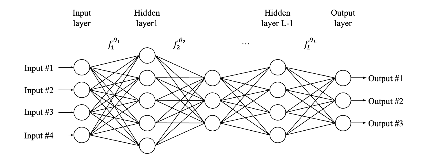
Figure 1: Structure of fully connected deep neural network.

Lemma 2.1

([32]) Let $d\geq 2,n\geq 2,m\geq 3,\sigma>0,a_{i},b_{i}\in\mathbb{Z}$ with $a_{i}<b_{i}$ for $1\leq i\leq d,D=\prod_{i=1}^{d}\left[a_{i},b_{i}\right]$ and $f\in H^{m}(D)$. Then for every $N\in\mathbb{N}$ with $N>5$ there exists a tanh neural network $u_{dnn}$ with two hidden layers, one of width at most $3\left\lceil\frac{m+n-2}{2}\right\rceil\left|P_{m-1,d+1}\right|+\sum_{i=1}^{d}\left(b_{i}-a_{i}\right)(N-1)$ and another of width at most $3\left\lceil\frac{d+n}{2}\right\rceil\left|P_{d+1,d+1}\right|N^{d}\prod_{i=1}^{d}\left(b_{i}-a_{i}\right)$, such that for $k=0,1,2$ the following inequalities hold

$$\left\|f-u_{dnn}\right\|_{H^{k}(D)}\leq 2^{k}3^{d}C_{k,m,d,f}(1+\delta)\ln^{k}\left(\beta_{k,\delta,d,f}N^{d+m+2}\right)N^{-m+k},$$

and where

$$C_{k,m,d,f} =\max_{0\leq l\leq k}\left(\begin{array}[]{c}d+l-1\\ l\end{array}\right)^{1/2}\frac{((m-l)!)^{1/2}}{\left(\left\lceil\frac{m-l}{d}\right\rceil!\right)^{d/2}}\left(\frac{3\sqrt{d}}{\pi}\right)^{m-l}|f|_{H^{m}(\Omega)},$$

$$\beta_{k,\delta,d,f} =\frac{5\cdot 2^{kd}\max\left\{\prod_{i=1}^{d}\left(b_{i}-a_{i}\right),d\right\}\max\left\{\|f\|_{W^{k,\infty}(\Omega)},1\right\}}{3^{d}\delta\min\left\{1,C_{k,m,d,f}\right\}}.$$

Moreover, the weights of $u_{dnn}$ scale as $O\left(N^{\gamma}+N\ln N\right)$ with $\gamma=\max\left\{m^{2}/n,d(2+m+d)/n\right\}$.

Lemma 2.1, which has been established in [32], shows that a two-hidden-layer tanh neural network is capable of achieving arbitrary smallness of $\|f-u_{dnn}\|_{H^{2}(D\times(0,T])}$ (i.e. $\left\|f-u_{dnn}\right\|_{H^{m}(\Omega)}<\epsilon$). Furthermore, it provides explicit bounds on the required network width. This illustrates the network’s strong ability to represent complex functions. In the subsequent section, we can utilize this approximation lemma to prove the upper bound on the residuals of the PDEs derived from the Physics-Informed Neural Network (PINN) (for more details, refer to Theorem 3.1 and Theorem 4.1).

2.3 Physics-informed neural networks for approximating the PDEs solution

Let $u_{dnn}(\bm{x},t;\theta)$ represent the approximated solution of the partial differential equation (PDE) (2.1) obtained from a neural network, where the network’s parameters $\theta=\{W^{L},b^{L}\}$ correspond to the neurons. These parameters can be updated using various optimization algorithms. In the field of physics-informed neural networks (PINNs) [18], these networks are used to solve PDEs by incorporating the governing equations as soft constraints in the optimization objective. This objective, denoted as $\mathcal{J}(u(\cdot;\theta))$, is defined as follows:

$$\mathcal{J}(u(\cdot;\theta))=\gamma_{int}\|R_{int}(\bm{x}_{int},t_{int};\theta)\|_{2,D\times(0,T]}^{2}+\gamma_{tb}\|R_{tb}(\bm{x}_{tb};\theta)\|_{2,D}^{2}+\gamma_{sb}\|R_{sb}(\bm{x}_{sb},t_{sb};\theta)\|_{2,\partial D\times[0,T]}^{2},$$ (2.4)

where $R_{int}(\bm{x}_{int},t_{int};\theta)=u_{t}(\bm{x}_{int},t_{int};\theta)-\mathcal{S}(u(\bm{x}_{int},t_{int};\theta))$, $R_{sb}(\bm{x}_{sb},t_{sb};\theta)=\mathcal{B}^{k}(u(\bm{x}_{sb},t_{sb};\theta))-0$, and $R_{tb}(\bm{x}_{tb};\theta)=u(\bm{x}_{tb};\theta)-u_{0}(\bm{x}_{tb})$ are the residual terms in the physics-informed neural network (PINN) framework. The hyperparameters, represented by $\gamma=\{\gamma_{int},\gamma_{sb},\gamma_{tb}\}$, serve as penalty coefficients that help balance the learning rate of each individual loss term. In this context, $\|\cdot\|_{2,D\times(0,T]}^{2}:=\int_{0}^{T}\int_{D}(\cdot)^{2}d\bm{x}dt$ and $\|\cdot\|_{2,D}^{2}:=\int_{D}(\cdot)^{2}d\bm{x}$ denote the usual $L^{2}$ norms over the domains $\Omega$ and $D$ respectively. In construct a reasonable numerical solution of (2.1) represented by the neural network, we consider the least squares problems on the loss function $\mathcal{J}(u(\cdot;\theta))$ with network parameter $\theta,$ this introduces a minimized optimization goal defined as

$$\theta^{*}=\arg\min_{\theta}\mathcal{J}(u(\cdot;\theta)),$$ (2.5)

where $u\left(\cdot;\theta^{*}\right)$ can be understood as the solution to the partial differential equations (PDEs) with optimized parameters. Consequently, PINNs (Physics-Informed Neural Networks) can be employed to solve PDEs using fully connected neural networks (FCNNs). Additionally, advancements in automatic differentiation technology [42] enable direct computation of the derivatives of the PDEs. By treating the solution of PDEs as a function approximation problem, optimization algorithms like gradient descent (GD), stochastic gradient descent (SGD), or Limited-memory Broyden-Fletcher-Goldfarb-Shanno (L-BFGS) can be employed to minimize the loss function and satisfy the physical constraints. In practice, it is necessary to discretize the integral norms in the objective function (2.4) using appropriate sampling methods, leading to an empirical approximation of the training loss as follows

$$\|R_{int}(\bm{x}_{int},t_{int};\theta)\|_{2,D\times(0,T]}^{2} =\frac{1}{N_{int}}\sum_{i=1}^{N_{int}}R_{int}^{2}(\bm{x}_{int}^{(i)},t_{int}^{(i)};\theta),$$ (2.6a)

$$\|R_{sb}(\bm{x}_{sb},t_{sb};\theta)\|_{2,\partial D\times(0,T]}^{2} =\frac{1}{N_{b}}\sum_{i=1}^{N_{sb}}R_{sb}^{2}(\bm{x}_{sb}^{(i)},t_{sb}^{(i)};\theta),$$ (2.6b)

$$\|R_{tb}(\bm{x}_{tb};\theta)\|_{2,{D\times\{0\}}}^{2} =\frac{1}{N_{tb}}\sum_{i=1}^{N_{tb}}R_{tb}^{2}(\bm{x}_{tb}^{(i)};\theta).$$ (2.6c)

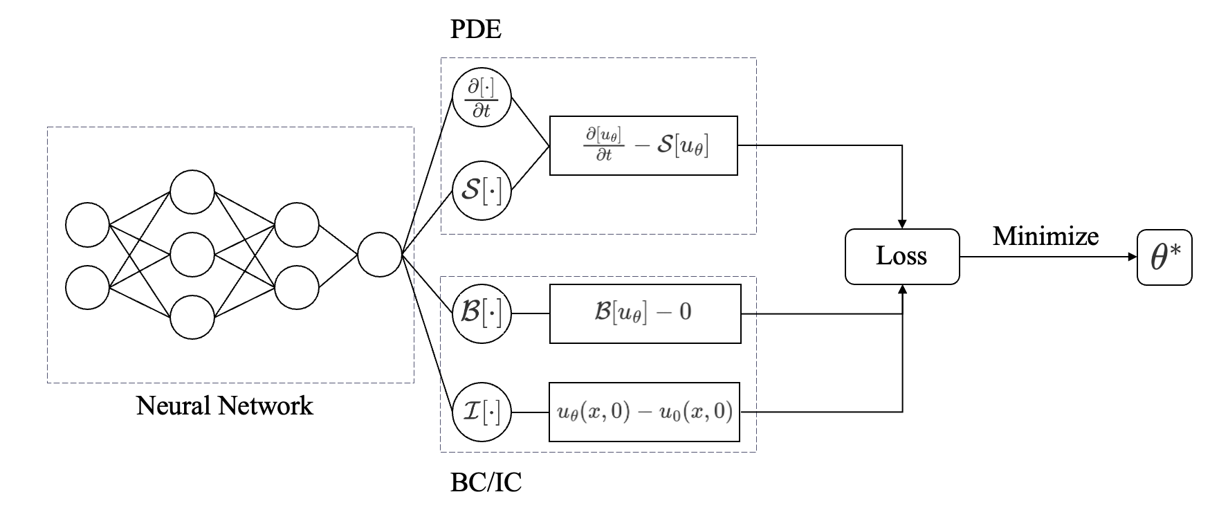
Figure 2: Schematic diagram of Physics-informed neural networks (PINNs).

Here, the training points $\{(\bm{x}_{int}^{(i)},t_{int}^{(i)})\}_{i=1}^{N_{int}}$, $\{(\bm{x}_{sb}^{(i)},t_{sb}^{(i)})\}_{i=1}^{N_{sb}}$ and $\{(\bm{x}_{tb}^{(i)})\}_{i=1}^{N_{tb}}$ are located in the interior, boundary and initial conditions of the computational domain, respectively. These points could be sampled using various methods such as uniform or Latin hypercube sampling (LHS). Afterward, the accuracy of the neural network’s predictions can be evaluated by comparing them to the exact solution. Let $u_{exact}$, $u_{dnn}$ represent the exact and predicted solutions from PINNs, respectively. In this work, we measure the accuracy using the relative $L^{2}$ error. The formula for the relative $L^{2}$ error is as follows:

$$\text{Relative }L^{2}{}\text{ error}=\frac{\sqrt{\sum_{i=1}^{N}\left|u_{dnn}(\bm{x}^{(i)},t^{(i)})-u_{exact}(\bm{x}^{(i)},t^{(i)})\right|^{2}}}{\sqrt{\sum_{i=1}^{N}\left|u_{exact}({\bm{x}}^{(i)},t^{(i)})\right|^{2}}},$$ (2.7)

where $\left\{(\bm{x}^{(i)},t^{(i)})\right\}_{i=1}^{N},(\bm{x}^{(i)},t^{(i)})\in D\times(0,T]$ represents a set of testing points. In order to compare our numerical solutions with the another one from the other methods, our reference solutions for the Allen–Cahn and Cahn–Hilliard equations are the ones obtained by a Chebyshev polynomial-based numerical algorithm [43], which ensures highly accurate solutions.

2.4 Self-adaptive learning using the Residuals-RAE weighting scheme

According to the study conducted by Mattey et al. (2022) [44], the std-PINN encounters challenges when dealing with highly nonlinear PDEs, such as the Allen–Cahn equation and Cahn–Hilliard equation. Figure 3 illustrates the predicted solution for these two equations using the vanilla PINNs with the specific forms of equations (3.11a) and (4.18a). It is evident that the vanilla PINNs fail to provide accurate predictions. To address this issue, recent research has explored potential solutions through the implementation of self-adaptive sample points or self-adaptive weights. The objective is to achieve fair training across the entire computational domain. However, it is important to note that previous experiments primarily utilized deep or deeper neural networks with multiple layers ($L\geq 3$). In contrast, our work needs to adopt a shallow neural network ($u_{\theta}$ with $L=2$, i.e., a single hidden layer) combined with a self-adaptive weighting scheme.

In our forthcoming research paper [18], we present a new formulation of the self-adaptive weighting scheme known as Residuals-RAE-PINNs, which incorporates the K-nearest algorithm. This approach considers the PDE residuals from neighboring points when calculating the weights. The research showcases that this algorithm provides exceptional stability, resulting in enhanced accuracy for difficult learning problems. Moreover, during the process of error analysis, a crucial issue arises when attempting to approximate the general loss using discrete samples from the domain. Therefore, it is essential to ensure that the self-adaptive weights are bounded and stable. This is a vital consideration in our decision to choose this framework. The primary difference in the modified training loss for Residuals-RAE-PINNs lies in its utilization of a weighted approach to evaluate PDE residuals, as opposed to the conventional MSE loss. More specifically, the modified training loss for interior points can be defined as follows:

$$\mathcal{J}(u(\cdot;\theta))=\gamma_{int}\|\hat{R}_{int}(\bm{x}_{int},t_{int};\theta)\|_{2,D\times(0,T]}^{2}+\gamma_{tb}\|R_{tb}(\bm{x}_{tb};\theta)\|_{2,D}^{2}+\gamma_{sb}\|R_{sb}(\bm{x}_{sb},t_{sb};\theta)\|_{2,\partial D\times(0,T]}^{2}.$$ (2.8)

In (2.8), we introduce the squared 2-norm of the modified internal residual $\|\hat{R}_{int}(\bm{x}_{int},t_{int};\theta)\|_{2,D\times(0,T]}^{2}$. The value of $\hat{R}_{int}^{(i)}$ can be estimated by multiplying the self-adaptive pointwise weights, $\lambda_{int}^{(i)}$, and the original internal residual, ${R}_{int}^{(i)}$. Here, $(\bullet)^{(i)}$ represents the index of the residual point sampled from the interior domain. The Residuals-RAE weighting scheme is designed to ensure stability in training and encourage the network to assign higher weights to sub-domains that are more difficult to learn. Initially, the Residuals-RAE-PINNs considers a simple weighting scheme:

$$w_{int}(\bm{x}_{int}^{(i)},t_{int}^{(i)};\theta)=\frac{|{R}_{int}(\bm{x}_{int}^{(i)},t_{int}^{(i)};\theta)|}{{\textstyle\sum_{i=1}^{N_{int}}}|{R}_{int}(\bm{x}_{int}^{(i)},t_{int}^{(i)};\theta)|}\cdot N_{int},\ i=1,2,\dots,N_{int},$$ (2.9)

where the normalization is applied here to obtain a normalized weights. However, the weights obtained from a simple weighting scheme may not be stable because the PDE residuals can change rapidly, potentially leading to failed training [45]. Inspired by the XPINNs [22], the Residuals-RAE PINNs [18] construct a set of near points for each interior points to average the weights from its neighboring points:

$$\bm{\lambda}_{Knear,r}^{(i)}=\frac{1}{k_{int}}\sum_{(\bm{x}_{int}^{(j)},t_{int}^{(j)})\in\bm{S}_{k_{int}}^{(i)}}w_{int}(\bm{x}_{int}^{(j)},t_{int}^{(j)};\theta),\ i=1,2,\dots,N_{int},$$ (2.10)

$$\bm{\lambda}_{int}^{k}=\beta\bm{\lambda}_{Knear,r}^{k}+(1-\beta)\bm{\lambda}^{k-1}_{int}.$$ (2.11)

Here, $\bm{S}_{k_{int}}^{(i)}$ represents the set of near points for the $i$-th point $(\bm{x}_{int}^{(i)},t_{int}^{(i)})$, where $k_{int}$ denotes the number of elements in the set. $\bm{\lambda}_{Knear,r}^{(i)}$ is a middle weights variable after normalization from its neighboring points. The superscript, $(\bullet)^{k}$ stands for the number of training iterations. The final $\bm{\lambda}^{k}_{int}$ is derived through a weighted sum of the previous weight $\bm{\lambda}^{k-1}_{int}$ from iteration $k-1$ and the normalized $\bm{\lambda}_{Knear,r}^{(i)}$ in the current $k$ iteration.

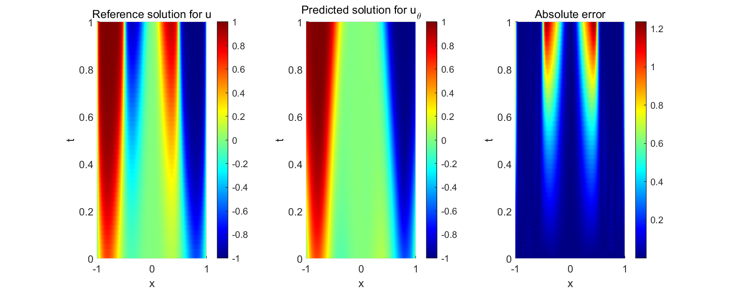
(a) Results for 1D Allen–Cahn equation (with initial condition $\#1$) using vanilla PINNs.

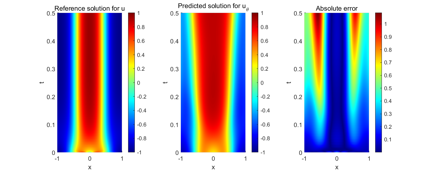
(b) Results for 1D Cahn–Hilliard equation using vanilla PINNs.

Figure 3: Results for solving 1D Allen–Cahn and 1D Cahn–Hilliard equations using vanilla PINN.

Further information on the design of a weighting scheme can be found in our upcoming publication titled ”Residuals-RAE-PINNs.” Moreover, Theorem 1.2 in Residuals-RAE-PINNs [18] demonstrates the expected value of $\bm{\lambda}^{k}$:

$$\mathbb{E}\left[\bm{\lambda}^{k}\right] =\mathbb{E}\left[\left(1-\beta\right)\sum_{i=1}^{k}\beta^{k-i}\cdot\bm{\lambda}_{Knear,r}^{(i)}\right]$$ (2.12)

$$=\mathbb{E}\left[\bm{\lambda}_{Knear,r}^{(i)}\right]\cdot\left(1-\beta\right)\sum_{i=1}^{k}\beta^{k-i}+\epsilon$$

$$=\mathbb{E}\left[\bm{\lambda}_{Knear,r}^{(i)}\right]\cdot\left(1-\beta^{k}\right)+\epsilon$$

$$=\frac{\sum_{(\bm{x}_{int}^{(j)},t_{int}^{(j)})\in\bm{S}_{k_{int}}^{(i)}}|{R}_{int}(\bm{x}_{int}^{(j)},t_{int}^{(j)};\theta)|}{{\textstyle\sum_{i=1}^{N_{int}}}|{R}_{int}(\bm{x}_{int}^{(i)},t_{int}^{(i)};\theta)|}\cdot\frac{N_{int}}{k_{int}}\cdot\left(1-\beta^{k}\right)+\epsilon.$$

Based on the derivation presented above, we can draw two conclusions. Firstly, the Residuals-RAE-PINN method achieves stability when the training process approaches convergence ($\epsilon=0$). Secondly, it is also possible to achieve this stability by utilizing a small learning rate or a learning rate decaying scheme, resulting in $\epsilon=0$. This property is particularly significant as it ensures that the pointwise weights defined within the interior domain remain stable as the number of training epochs increases.

Furthermore, the adjusted generalization error of a Residuals-RAE-PINN can be determined by

$$\mathcal{E}_{G}(\theta)^{2}=\int_{D\times[0,T]}\left|R_{int}(\bm{x}_{int},t_{int})\right|^{2}\mathrm{~{}d}\bm{x}\mathrm{~{}d}t+\int_{D}\left|R_{tb}(\bm{x}_{tb})\right|^{2}\mathrm{~{}d}s(\bm{x})\mathrm{d}t+\int_{\partial D\times(0,T]}\left|R_{sb}(\bm{x}_{sb},t_{sb})\right|^{2}\mathrm{~{}d}\bm{x}.$$ (2.13)

To simplify the calculation of the generalization error, we can approximate the integrals in (2.13) using numerical quadrature rules, as explained in Lemma B.6. As a result, we define the training loss as follows:

$$\mathcal{E}_{T}(\theta,S)^{2}=\mathcal{E}_{T}^{int}(\theta,S_{int})^{2}+\mathcal{E}_{T}^{tb}(\theta,S_{tb})^{2}+\mathcal{E}_{T}^{sb}(\theta,S_{sb})^{2},$$ (2.14)

where

$$\mathcal{E}_{T}^{int}(\theta,S_{int})^{2}= ~{}\sum_{i=1}^{N_{int}}\lambda_{int}^{(i)}|R_{int}(x_{int}^{(i)},t_{int}^{(i)})|^{2},$$

$$\mathcal{E}_{T}^{tb}(\theta,S_{tb})^{2}= ~{}\sum_{i=1}^{N_{tb}}\lambda_{tb}^{(i)}|R_{tb}(x_{tb}^{(i)})|^{2},$$

$$\mathcal{E}_{T}^{sb}(\theta,S_{sb})^{2}= ~{}\sum_{i=1}^{N_{sb}}\lambda_{sb}^{(i)}|R_{sb}(x_{sb}^{(i)},t_{sb}^{(i)})|^{2}.$$

Here, the weights $\lambda_{int}^{(i)}$ in (2.11) are obtained from the Residuals-RAE-PINNs, while the other weights $\lambda_{sb}^{(i)}$ and $\lambda_{tb}^{(i)}$ are related to the quadrature rule. The definition of the residuals remains the same as in (2.4).

3 Physics Informed Neural Networks for Approximating the Allen–Cahn Equation

3.1 Allen–Cahn Equation

Let us consider the general form of the Allen–Cahn equation defined in the domain $\Omega:=D\times(0,T]$, where $D\subset\mathbb{R}^{d}$ and $d\in\mathbb{N}$. The Allen–Cahn equation is given by:

$$u_{t}-c_{1}^{2}\nabla^{2}u+f(u)=0,\quad t\in(0,T],\quad\bm{x}\in D$$ (3.1a)

$$u(\bm{x},0)=\psi(\bm{x}),\quad\bm{x}\in D$$ (3.1b)

$$u(\bm{x},t)=u(-\bm{x},t),\quad t\in(0,T],\quad\bm{x}\in\partial D$$ (3.1c)

$$\nabla u(\bm{x},t)=\nabla u(-\bm{x},t),\quad t\in(0,T],\quad\bm{x}\in\partial D$$ (3.1d)

Here, the diffusion coefficients $c_{1}$ is a constant, the nonlinear term $f(u)$ is a polynomial in $u,$ and $u(\bm{x},t)$ represents the unknown field solution, and $\psi$ denotes the initial distributions for $u$ at $t=0.$ The boundary conditions have been assumed to be periodic.

Furthermore, we are able to derive the following regularity results.

Lemma 3.1

[46] Let $r\geq 1$, $\psi\in H^{r}(\Omega)$ and $f\in C^{r}(\mathbb{R})$, then for every $|\psi|<1$, $\psi\in H^{r}(\Omega)$ and $T>0$ there exists a weak solution $u\in C\left((0,T];H^{r}(\Omega)\right)$ and $\partial_{t}u\in C\left((0,T];H^{r-1}(D)\right)$ to Allen–Cahn equation 3.1 that

$$\left\langle\partial_{t}u,v\right\rangle+c^{2}(\nabla u,\nabla v)=-(f(u),v)$$

for every $t\in(0,T]$ and every $v\in H^{1}(\Omega)$.

Lemma 3.2

Let $k\in\mathbb{N}$, $\psi\in H^{r}(D)$ and $f\in C^{r}(\mathbb{R})$ with $r>\frac{d}{2}+k$, then there exists $T>0$ and a weak solution $u$ to Allen–Cahn equation 3.1 such that $u(t=0)=\psi$, $u\in C^{k}((0,T]\times D)$ and $\partial_{t}u\in C^{k-1}((0,T]\times D)$.

The proof for Lemma 3.2 is provided in the Appendix C.

3.2 Physics Informed Neural Networks

In this section, we present a physics-informed neural network that can be used to estimate the solution of partial differential equations (PDEs). The network, denoted as $u_{\theta}:\Omega\rightarrow\mathbb{R}$, is parameterized by $\theta$ and operates on the domain $\Omega:=D\times(0,T]$. Subsequently, we can derive the following:

$$R_{\text{int }}^{AC}\left[u_{\theta}\right](\bm{x},t)=\partial_{t}u_{\theta}-c_{1}^{2}\nabla^{2}u_{\theta}+f(u_{\theta}),$$ (3.2a)

$$R_{tb}^{AC}\left[u_{\theta}\right](\bm{x})=u_{\theta}(\bm{x},0)-\psi(\bm{x}),$$ (3.2b)

$$R_{sb1}^{AC}\left[u_{\theta}\right](\bm{x},t)=u_{\theta}(\bm{x},t)-u_{\theta}(-\bm{x},t),$$ (3.2c)

$$R_{sb2}^{AC}\left[u_{\theta}\right](\bm{x},t)=\nabla u_{\theta}(\bm{x},t)-\nabla u_{\theta}(-\bm{x},t).$$ (3.2d)

The equations above can be derived promptly. PINNs convert the task of solving equations into an approximation problem, resulting in the generalization error as below

$$\mathcal{E}^{AC}_{G}(\theta)^{2}= \int_{D}|R_{tb}^{AC}|^{2}d\bm{x}+\int_{0}^{T}\int_{D}|R_{int}^{AC}|^{2}d\bm{x}dt$$ (3.3)

$$+c_{1}^{2}\tilde{C}|T|^{1/2}(\int_{0}^{T}\int_{\partial D}|R_{sb1}^{AC}|^{2}ds(\bm{x})dt)^{1/2}+c_{1}^{2}\tilde{C}|T|^{1/2}(\int_{0}^{T}\int_{\partial D}|R_{sb2}^{AC}|^{2}ds(\bm{x})dt)^{1/2},$$

where $\tilde{C}=|\partial D|^{\frac{1}{2}}(||{u}||_{C^{1}(\partial D\times(0,T])}+||{u}_{\theta}||_{C^{1}(\partial D\times(0,T])})$.

In practice, the estimation of the generalization error $\mathcal{E}_{G}^{AC}(\theta)$ can be approximated using appropriate numerical quadrature rules and the training points from the sample method. The training set, denoted as $\mathcal{S}^{AC}$, consists of suitable quadrature points for the inner domain, boundary, and initial conditions. This set can be further divided into three subsets: $\mathcal{S}^{AC}_{int}=\{(\bm{x}^{(i)}_{int},t^{(i)}_{int})\}_{i=1}^{N_{int}}$, $\mathcal{S}^{AC}_{tb}=\{(\bm{x}^{(i)}_{tb})\}_{i=1}^{N_{tb}}$, and $\mathcal{S}^{AC}_{sb}=\{(\bm{x}^{(i)}_{sb},t^{(i)}_{sb})\}_{i=1}^{N_{sb}}$. Here, $N_{int}$, $N_{sb}$, and $N_{tb}$ represent the number of training points for the governing equation, boundary conditions, and initial conditions, respectively. The training error can then be expressed as follows:

$$\mathcal{E}^{AC}_{T}(\theta,\mathcal{S}^{AC})^{2}:= \sum_{i=1}^{N_{tb}}\lambda_{tb}^{(i)}|R_{tb}^{AC}(\bm{x}_{tb}^{(i)})|^{2}+\sum_{i=1}^{N_{int}}\lambda_{int}^{(i)}|R_{int}^{AC}(\bm{x}_{int}^{(i)},t_{int}^{(i)})|^{2}$$ (3.4)

$$+c_{1}^{2}\tilde{C}|T|^{1/2}(\sum_{i=1}^{N_{sb}}\lambda_{sb}^{(i)}|R_{sb1}^{AC}(\bm{x}_{sb}^{(i)},t_{sb}^{(i)})|^{2})^{1/2}+c_{1}^{2}\tilde{C}|T|^{1/2}(\sum_{i=1}^{N_{sb}}\lambda_{sb}^{(i)}|R_{sb1}^{AC}(\bm{x}_{sb}^{(i)},t_{sb}^{(i)})|^{2})^{1/2}.$$

Here, we use $\hat{u}=u_{\theta}-u$ to represent the numerical error between the predicted solution from PINNs and the exact solution. Then we define the total error of PINNs with the following form:

$$\mathcal{E}^{AC}(\theta)^{2}=\|\hat{u}(\bm{x},t)\|^{2}_{L^{2}{(D\times(0,T])}}+2c_{1}^{2}\int_{0}^{T}\|\nabla\hat{u}(\bm{x},t)\|^{2}_{L^{2}{(D\times(0,t])}}dt.$$ (3.5)

In the next section, we will undertake a detailed analysis of $\mathcal{E}^{AC}(\theta)^{2}$.

3.3 Error Analysis

The Allen–Cahn equations and the definitions for different residuals can be re-expressed as follows:

$$R_{\text{int}}^{AC}(\bm{x},t)=\hat{u}_{t}-c_{1}^{2}\nabla^{2}\hat{u}-f(u)+f(u_{\theta}),$$ (3.6a)

$$R_{tb}^{AC}(\bm{x})=\hat{u}(\bm{x},0),$$ (3.6b)

$$R_{sb1}^{AC}(\bm{x},t)=\hat{u}(\bm{x},t)-\hat{u}(-\bm{x},t),$$ (3.6c)

$$R_{sb2}^{AC}(\bm{x},t)=\nabla\hat{u}(\bm{x},t)-\nabla\hat{u}(-\bm{x},t),$$ (3.6d)

where $\hat{u}=u_{\theta}-u$ is substituted into (3.2) to obtain the above equations.

3.3.1 Bound on the Residuals

Theorem 3.1

Let $d,r,k\in\mathbb{N}$ with $k\geq 3$. Let $\psi\in H^{r}(D)$ and $f\in C^{k-1}\left((0,T];H^{r-1}(D)\right)$ with $r>\frac{d}{2}+k$. For every integer $N>5$, there exists a tanh neural network $u_{\theta}$ with two hidden layers, each with a width of at most $3\left\lceil\frac{k+n-2}{2}\right\rceil\left|P_{k-1,d+2}\right|+\lceil NT\rceil+d(N-1)$, such that

$$\left\|R_{\text{int }}^{AC}\right\|_{L^{2}(\Omega)},\left\|R_{sb2}^{AC}\right\|_{L^{2}(\partial D\times(0,T])}\lesssim\ln^{2}\left(N\right)N^{-k+2},$$ (3.7a)

$$\left\|R_{sb1}^{AC}\right\|_{L^{2}(\partial D\times(0,T])},\left\|R_{\text{tb }}^{AC}\right\|_{L^{2}(D)}\lesssim\ln\left(N\right)N^{-k+1}.$$ (3.7b)

The proof for Theorem 3.1 is provided in the Appendix C.

In Theorem 3.1 above, we provide evidence that increasing the value of $N$ leads to a reduction in the residuals, namely $\left\|R_{\text{int }}^{AC}\right\|_{L^{2}(\Omega)}$, $\left\|R_{sb2}^{AC}\right\|_{L^{2}(\partial D\times(0,T])}$, $\left\|R_{sb1}^{AC}\right\|_{L^{2}(\partial D\times(0,T])}$, and $\left\|R_{tb}^{AC}\right\|_{L^{2}(D)}$. Consequently, this implies that the generalization error $\mathcal{E}^{AC}_{G}(\theta)^{2}$ in (3.3), can also be made arbitrarily small.

3.3.2 Bounds on the Total Approximation Error

In the following section, we will demonstrate that the total error $\mathcal{E}^{AC}(\theta)^{2}$ can be controlled by generalization error $\mathcal{E}^{AC}_{G}(\theta)^{2}$. Furthermore, we will establish that the total error $\mathcal{E}^{AC}(\theta)^{2}$ can be made arbitrarily small, provided that the training error $\mathcal{E}^{AC}_{T}(\theta,S^{AC})^{2}$ is kept sufficiently small and the sample set sufficiently large.

Theorem 3.2

Let $d\in\mathbb{N}$ and $u\in C^{1}(\Omega)$ be the classical solution to the Allen–Cahn equations. Let $u_{\theta}$ denote the PINN approximation with parameter $\theta$. Then the following relation holds,

$$\mathcal{E}^{AC}(\theta)^{2}=\|\hat{u}(\bm{x},t)\|^{2}_{L^{2}(D\times(0,T])}+2c_{1}^{2}\int_{0}^{T}\|\nabla\hat{u}(\bm{x},t)\|^{2}_{L^{2}(D\times(0,t])}dt\leq C_{G}T\exp((1+2M)T),$$ (3.8)

where

$$C_{G}=\mathcal{E}^{AC}_{G}(\theta)^{2}=\int_{D}|R_{tb}^{AC}|^{2}d\bm{x}+\int_{0}^{T}\int_{D}|R_{int}^{AC}|^{2}d\bm{x}dt +c_{1}^{2}\tilde{C}|T|^{1/2}(\int_{0}^{T}\int_{\partial D}|R_{sb1}^{AC}|^{2}ds(\bm{x})dt)^{1/2}$$

$$+c_{1}^{2}\tilde{C}|T|^{1/2}(\int_{0}^{T}\int_{\partial D}|R_{sb2}^{AC}|^{2}ds(\bm{x})dt)^{1/2},$$

and $\tilde{C}=|\partial D|^{\frac{1}{2}}(||{u}||_{C^{1}(\partial D\times(0,T])}+||{u}_{\theta}||_{C^{1}(\partial D\times(0,T])})$ .

The proof for Theorem 3.2 is provided in the Appendix C.

Theorem 3.3

Let $d\in\mathbb{N}$ and $T>0$. Let $u\in C^{4}(\Omega)$ be the classical solution of the Allen–Cahn equations, and let $\left(u_{\theta}\right)$ denote the PINN approximation. The total error satisfies

$$\mathcal{E}^{AC}(\theta)^{2}=\|\hat{u}(\bm{x},t)\|^{2}_{L^{2}(D\times(0,T])}+2c_{1}^{2}\int_{0}^{T}\|\nabla\hat{u}(\bm{x},t)\|^{2}_{L^{2}(D\times(0,t])}dt \leq C_{T}T\exp((1+2M)T)$$ (3.9)

$$=\mathcal{O}(\mathcal{E}^{AC}_{T}(\theta,\mathcal{S}^{AC})^{2}+M_{tb}^{-\frac{2}{d}}+M_{int}^{-\frac{2}{d+1}}+M_{sb}^{-\frac{2}{d}})$$

The constant $C_{T}$ is defined as

$$C_{T}= C_{\left[(R_{tb}^{AC})^{2}\right]}M_{tb}^{-\frac{2}{d}}+\mathcal{Q}_{M_{tb}}^{D}\left[(R_{tb}^{AC})^{2}\right]+C_{\left[(R_{int}^{AC})^{2}\right]}M_{int}^{-\frac{2}{d+1}}+\mathcal{Q}_{M_{int}}^{\Omega}\left[(R_{int}^{AC})^{2}\right]$$ (3.10)

$$+c_{1}^{2}\tilde{C}|T|^{1/2}(C_{[\left(R_{sb1}^{AC})^{2}\right]}M_{sb}^{-\frac{2}{d}}+\mathcal{Q}_{M_{sb}}^{D\times\left(0,T\right]}[\left(R_{sb1}^{AC})^{2}\right])^{1/2}$$

$$+c_{1}^{2}\tilde{C}|T|^{1/2}(C_{\left[\left(R_{sb2}^{AC}\right)^{2}\right]}M_{sb}^{-\frac{2}{d}}+\mathcal{Q}_{M_{sb}}^{D\times\left(0,T\right]}[\left(R_{sb2}^{AC})^{2}\right])^{1/2},$$

where $\tilde{C}=|\partial D|^{\frac{1}{2}}(||{u}||_{C^{1}(\partial D\times(0,T])}+||{u}_{\theta}||_{C^{1}(\partial D\times(0,T])})$.

The proof for Theorem 3.3 is provided in the Appendix C.

By utilizing Theorem 3.2 in conjunction with Theorem 3.3, we can establish that the total approximation error $\mathcal{E}(\theta)^{2}$ could be controlled by both the training error $\mathcal{E}^{AC}_{T}(\theta,\mathcal{S}^{AC})^{2}$ and the size of the training set.

3.4 Numerical Examples

3.4.1 1D Allen–Cahn equation

In this section, we will simulate the Allen–Cahn equation, which is a challenging partial differential equation (PDE) for classical Physics-Informed Neural Networks (PINNs) due to its stiffness and sharp transitions in the spatio-temporal domain. Considering the space-time domain $D\times(0,T]=[-1,1]\times(0,1]$, the Allen–Cahn equation we will be discussing is for a specific one-dimensional time variation. It is accompanied by the following initial and periodic boundary conditions, as defined below:

$$u_{t}-0.001u_{xx}+3u^{3}-3u=0,\quad(x,t)\in D\times(0,T]$$ (3.11a)

$$u(x,0)=x^{2}sin(2\pi x),\quad(x,t)\in D\times\{0\}$$ (3.11b)

$$u(-x,t)=u(x,t),\quad(x,t)\in\partial D\times(0,T]$$ (3.11c)

$$\nabla u(-x,t)=\nabla u(x,t),\quad(x,t)\in\partial D\times(0,T].$$ (3.11d)

The initial condition in (3.11b) will be denoted as initial condition $\#1$ in the following discussions. What’s more, we also consider the initial condition $\#2$ given by:

$$u(x,0)=cos(\pi x)-exp(-4(\pi x)^{2}).$$ (3.12)

The Allen–Cahn equations will be denoted as AC-I1 and AC-I2, corresponding to initial conditions $\#1$ and $\#2$ respectively. To apply the Residuals-RAE method in solving the equation, we define the loss function as follows (using AC-I1 as an example):

$$\mathcal{L}(\theta) =\gamma_{int}\cdot\mathcal{L}_{int}(\theta)+\gamma_{tb}\cdot\mathcal{L}_{tb}(\theta)+\gamma_{sb}\cdot\mathcal{L}_{sb}(\theta)$$

$$=\gamma_{int}\cdot\frac{1}{N_{int}}\sum_{i=1}^{N_{int}}\hat{\lambda}_{int}^{(i)}|u_{t}(x_{int}^{(i)},t_{int}^{(i)})+0.001u_{xx}(x_{int}^{(i)},t_{int}^{(i)})+3u^{3}(x_{int}^{(i)},t_{int}^{(i)})-3u(x_{int}^{(i)},t_{int}^{(i)})|^{2}$$

$$+\gamma_{tb}\cdot\frac{1}{N_{tb}}\sum_{i=1}^{N_{tb}}|u(x_{tb}^{(i)},0)-u_{0}(x_{tb}^{(i)})|^{2}.$$

$$+\gamma_{sb}\cdot\frac{1}{N_{sb}}\sum_{i=1}^{N_{sb}}(|u(-x_{sb}^{(i)},t_{sb}^{(i)})-u(x_{sb}^{(i)},t_{sb}^{(i)})|^{2}+|\nabla u(-x_{sb}^{(i)},t_{sb}^{(i)})-\nabla u(x_{sb}^{(i)},t_{sb}^{(i)})|^{2}),$$ (3.13)

where the weights for different terms are $\gamma_{int}=1$, $\gamma_{sb}=1$ and $\gamma_{tb}=100$. When the point-wise weights $\hat{\lambda}_{int}^{(i)}$ of interior points are set to 1, the loss function reduces to the classical MSE loss. During training, a fully-connected neural network architecture with a depth of 2 and a width of 128 is used. To optimize the modified loss function, a combination of $30,000$ iterations using the Adam algorithm and $1,000$ iterations using the L-BFGS algorithm are utilized. Alternatively, the training may terminate prematurely if the loss decreases by less than $10^{-7}$ between two consecutive epochs. We randomly sample $N_{int}=10,000$, $N_{sb}=256$, $N_{tb}=512$ collation points from the computational domain using the latin hypercube sampling (LHS) approach.

To implement the Residuals-RAE weighting scheme for pointwise weights $\hat{\lambda}_{int}^{(i)}$ of residual points, the hyper-parameter $k_{int}$ in (2.11) is set to 50. This hyper-parameter determines the influence from the nearest points when measuring the pointwise weights. The relative L2 errors of Residuals-RAE in the Allen–Cahn equation with initial conditions $\#1$ and $\#2$ are $8.09e-03$, $6.53e-02$ respectively (see Fig. 4). The reference data are obtained using spectral methods with the Chebfun package. Moreover, the point-wise absolute error distributions in the domain tend to accumulate in sub-regions where the PDE solution exhibits sharp transitions. The phenomenon is often observed in physics-informed neural networks (PINNs).

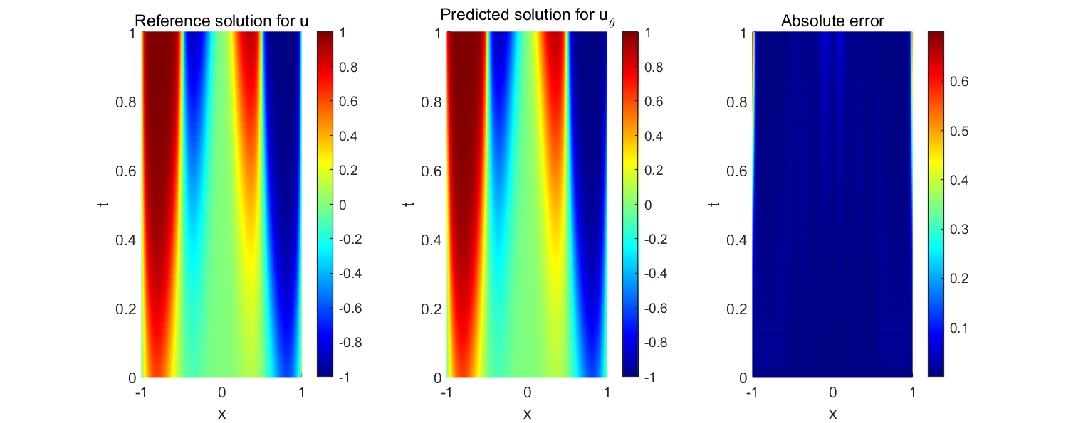
(a) Results for 1D Allen–Cahn equation (with initial condition $\#1$ ($u(0,x)=x^{2}sin(2\pi x)$) using Residuals-RAE PINNs.

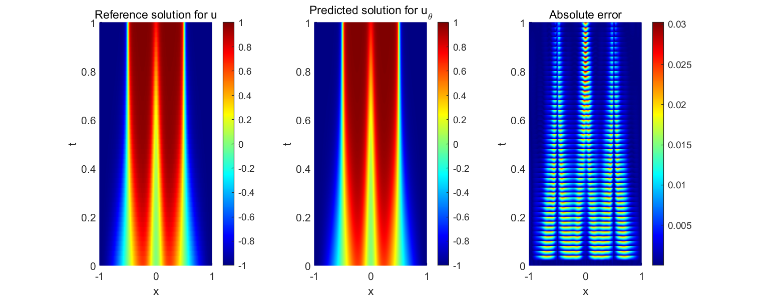
(b) Results for 1D Allen–Cahn equation (with initial condition $\#2$ $u(0,x)=u(x,0)=cos(\pi x)-exp(-4(\pi x)^{2}$) using Residuals-RAE PINNs.

Figure 4: Results for solving 1D Allen–Cahn equation using Residuals-RAE. $1^{st}$ column: Reference $u$, $2^{nd}$ column: the predicted $u$ from Residuals-RAE, $3^{rd}$ column: absolute pointwise error (relative $L^{2}$ error: $8.09e-03$ (initial condition $\#1$), and $6.53e-02$ (initial condition $\#2$).

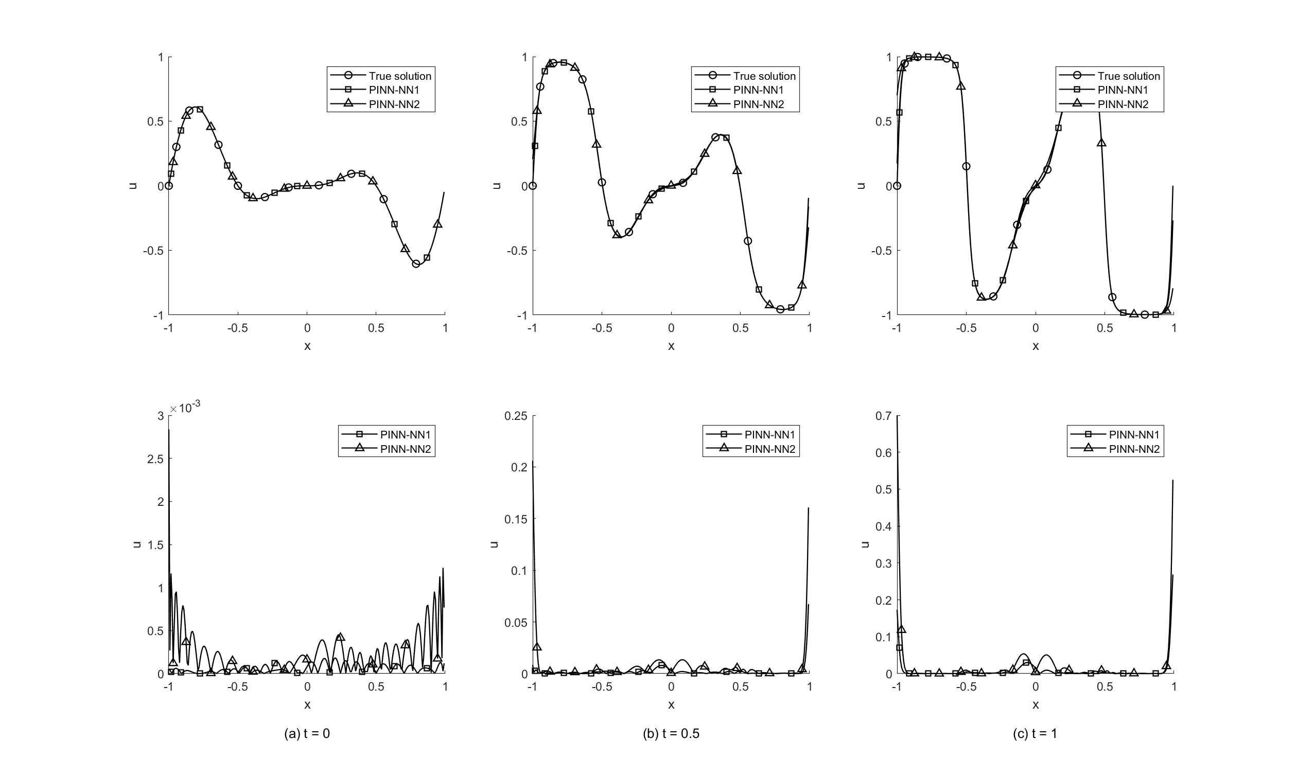
(a) Reference and Residuals-RAE-PINN predicted solutions (neurons per layer $\#1$ and $\#2$) of the 1D Allen–Cahn equation (initial condition $\#$ 1) at different time snapshots (a) $t=0$, (b) $t=0.5$, (c) $t=1$.

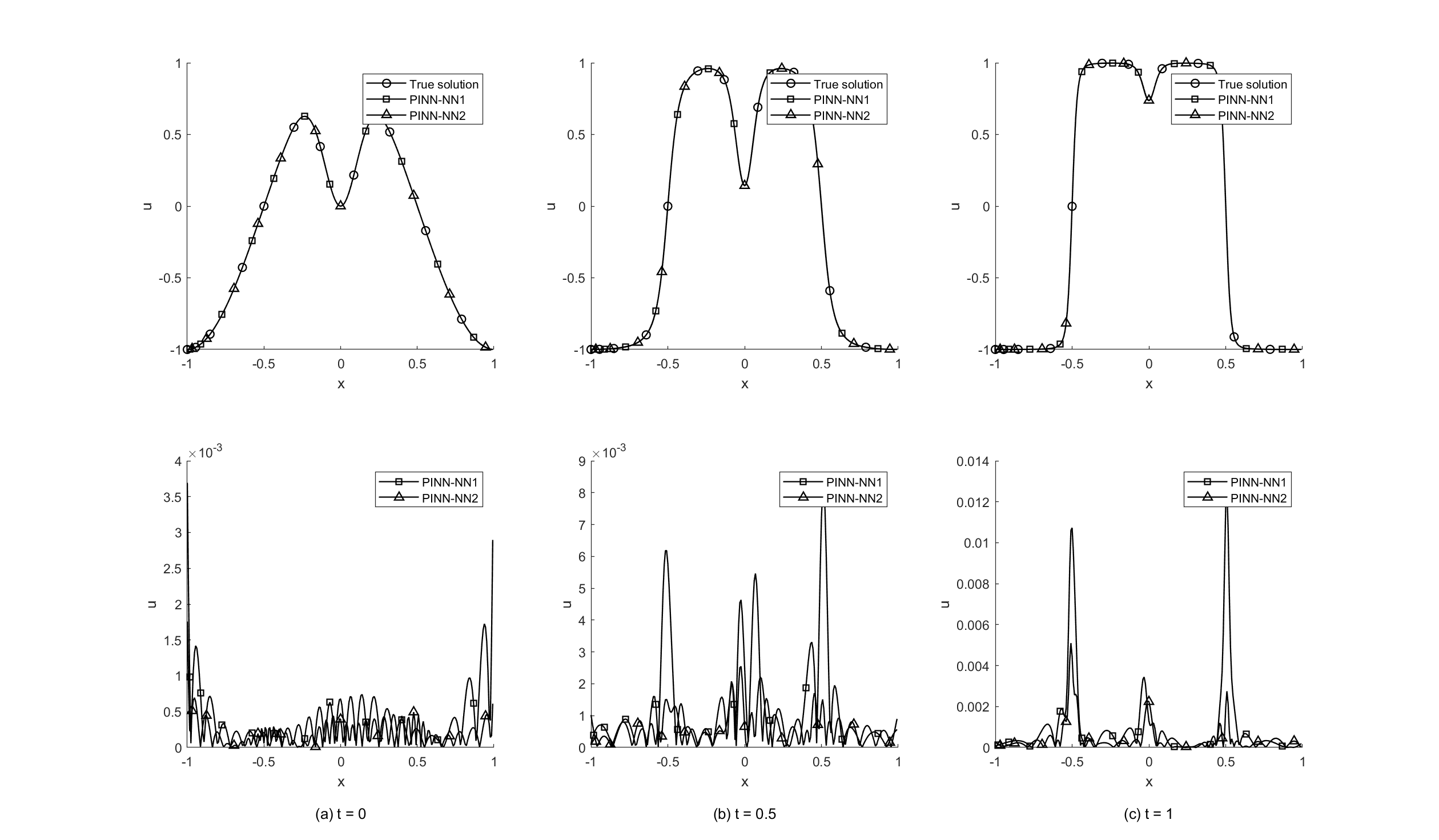
(b) Reference and Residuals-RAE-PINN predicted solutions (neurons per layer $\#1$ and $\#2$) of the 1D Allen–Cahn equation (initial condition $\#$ 2) at different time snapshots (a) $t=0$, (b) $t=0.5$, (c) $t=1$.

Figure 5: Results for solving 1D Allen–Cahn equation using Residuals-RAE.

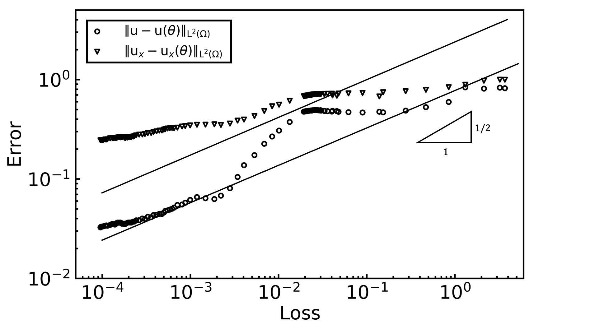
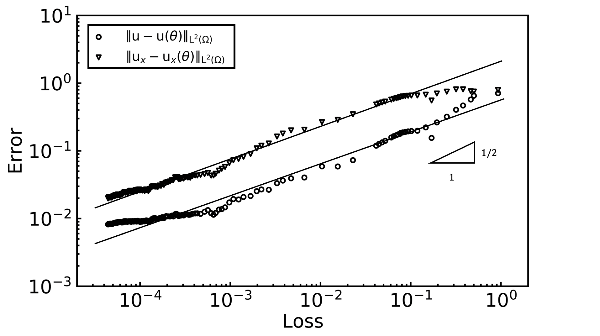
Figure 6: 1D Allen–Cahn equation: The evolution of $l^{2}$ solution errors for $u$ and $u_{x}$ as a function of the training loss value using Residuals-RAE. Left: 1D Allen–Cahn equation with initial condition $\#1$. Right: 1D Allen–Cahn equation with initial condition $\#2$.

Fig. 5 presents the numerical outcomes achieved through the Residuals-RAE-PINNs method at different time snapshots ($t=0,0.5,$ and $1.0$). In order to examine the impact of the width of the neural network, we also provide the numerical results for this problem by varying the number of neurons in the 2-layer neural network. Specifically, PINN-NN1 employs a neural network with 256 neurons per layer, while PINN-NN2 adopts a neural network with 128 neurons per layer. The performance of these networks is evaluated against the reference solution, with the top row of graphs illustrating the solutions at the specified time intervals and the bottom row showcasing the corresponding errors. The numerical findings indicate that the wider neural network (PINN-NN1) performs better, displaying a closer fit to the true solution, and smaller errors compared to the narrower network (PINN-NN2). This is a common outcome in machine learning, where increasing the capacity of a model (such as increasing the number of neurons) can lead to better approximation of complex functions, up to a point of diminishing returns where overfitting can become an issue.

Table 1: Description of training data for 1D Allen–Cahn equation (AC-I1, AC-I2).

$$\begin{array}[]{lll}\hline\cr N_{tb}&\text{ Initial collocation points }&512\\ N_{sb}&\text{ Boundary collocation points }&256\\ N_{int}&\text{ Residual collocation points }&10,000\\ \hline\cr\end{array}$$

In Fig. 6, we analyze the behavior of errors for $u,\frac{\partial u}{\partial t},\frac{\partial u}{\partial x}$ in order to assess the convergence rate during training. The errors are plotted against the corresponding values of the loss function used in training, with a logarithmic scale applied. The lines labeled $1/2$ and $1$ are included as reference slopes for comparison. Based on the figure, it is evident that for PINNs the scaling essentially follows the square root relation. This scaling indicates that as the training loss decreases, the errors also decrease, although at a slower rate. This observation is commonly encountered in neural network training, where improvements in the loss function lead to improved prediction accuracy. The alignment between the numerical results of training dynamics and the theoretical prediction provides numerical evidence that supports the previously presented theory (Theorem 3.3), specifically regarding the residuals-rae training loss function.

3.4.2 2D Allen–Cahn equation

Here, we also consider the 2D Allen–Cahn equation defined on the computational domain as $D\times(0,T]=[0,1]^{2}\times(0,5]$, and the boundary conditions have been considered to be periodic. Then we can have the following formulation

$$u_{t}(x,y,t)-\lambda\varepsilon^{2}\Delta u(x,y,t)+\lambda u(x,y,t)^{3}-\lambda u(x,y,t)=0,\qquad(x,y,t)\in D\times(0,T]$$ (3.14a)

$$u(x,y,0)=u_{0},\qquad(x,y,t)\in D\times\{0\}$$ (3.14b)

$$u^{(d-1)}(x,y,t)=u^{(d-1)}(-x,-y,t),\qquad(x,y,t)\in\partial D\times(0,T]\qquad(d=1,2)$$ (3.14c)

where the physical parameters $\lambda=10,\varepsilon=0.025$, and the initial condition for $u$ was given by $u(x,y,t=0)=\tanh\left(\frac{0.35-\sqrt{(x-0.5)^{2}+(y-0.5)^{2}}}{2\varepsilon}\right)$. In this problem, we consider the modified loss function with self-adaptive weights used here, which could be specified as below

$$\mathcal{L}(\theta) =\gamma_{int}\cdot\mathcal{L}_{int}(\theta)+\gamma_{tb}\cdot\mathcal{L}_{tb}(\theta)+\gamma_{sb}\cdot\mathcal{L}_{sb}(\theta)$$

$$=\gamma_{int}\cdot\frac{1}{N_{int}}\sum_{i=1}^{N_{int}}\hat{\lambda}_{int}^{(i)}\left|u_{t}(x_{int}^{(i)},y_{int}^{(i)},t_{int}^{(i)})-\lambda\varepsilon^{2}\Delta u(x_{int}^{(i)},y_{int}^{(i)},t_{int}^{(i)})+\lambda u(x_{int}^{(i)},y_{int}^{(i)},t_{int}^{(i)})^{3}-\lambda u(x_{int}^{(i)},y_{int}^{(i)},t_{int}^{(i)})\right|^{2}$$

$$+\gamma_{tb}\cdot\frac{1}{N_{tb}}\sum_{i=1}^{N_{tb}}\left|u(x_{tb}^{(i)},y_{tb}^{(i)},0)-u_{0}(x_{tb}^{(i)},y_{tb}^{(i)},0)\right|^{2}$$

$$+\gamma_{sb}\cdot\frac{1}{N_{sb}}\sum_{i=1}^{N_{sb}}(\left|u^{(1)}(x_{sb}^{(i)},y_{sb}^{(i)},t_{sb}^{(i)})-u^{(1)}(-x_{sb}^{(i)},-y_{sb}^{(i)},t_{sb}^{(i)})\right|^{2}+\left|u^{(0)}(x_{sb}^{(i)},y_{sb}^{(i)},t_{sb}^{(i)})-u^{(0)}(-x_{sb}^{(i)},-y_{sb}^{(i)},t_{sb}^{(i)})\right|^{2}).$$ (3.15)

Here, the weights for the loss terms, namely $\gamma_{int},\gamma_{sb},\gamma_{tb}$, are set to $1,1,100$, respectively. To obtain point-wise weights, the residuals-RAE weighting scheme is employed. When considering the influence from nearby points during training, the number of k-nearest points is set to 50 for interior points. The input layer of the PINN structure consists of 3 neurons. For solving the PDEs, a neural network with a depth of 2 and a width of 128 is utilized, which is the same as the one used for solving the 1D Allen–Cahn equation. In addition, we sample a total of $25,600$ points from the interior domain, $512$ points from the boundary, and $1,024$ points from the initial conditions to train the network. The training process consists of $100,000$ ADAM iterations, with an initial learning rate of $0.001$. To ensure the stability of training for this complex problem, we also incorporate exponential learning rate decay, with a decay rate of $0.9$ applied after every $5,000$ training iterations.

Table 2: Description of training data for 2D Allen–Cahn equation.

$$\begin{array}[]{lll}\hline\cr N_{tb}&\text{ Initial collocation points }&1024\\ N_{sb}&\text{ Boundary collocation points }&512\\ N_{int}&\text{ Residual collocation points }&25,600\\ \hline\cr\end{array}$$

To assess the accuracy of the PINN method, we also present the evolution of the function $u(x,y,t)$ over time by visualizing snapshots at t = 0, 2.5, and 5 for the 2D Allen–Cahn equations (see Fig. 8). The residuals-RAE PINN successfully captures the solution and shows a close match with the reference solution obtained from the spectral method in the Chebfun package. It is worth noting that the accurate characterization of the weights is crucial for the PINN algorithm to produce an accurate approximation.

The figure shown in Fig. 7 illustrates the errors in $u$, $u_{x}$, and $u_{y}$ plotted against the corresponding values of the loss function obtained during the training of the neural network. The straight line marked with the labels $1/2$ indicates the theoretical reference slopes that the training dynamics might be expected to follow if the error scales with the square root of the loss. This type of plot is commonly used to demonstrate the efficiency and convergence behavior of neural network training, specifically in the context of solving PDEs where derivatives are also of interest. The alignment of the training dynamics with the reference lines would typically indicate that the neural network training is consistent with theoretical expectations as suggested in Theorem 3.3 for scaling between the training loss and solution errors.

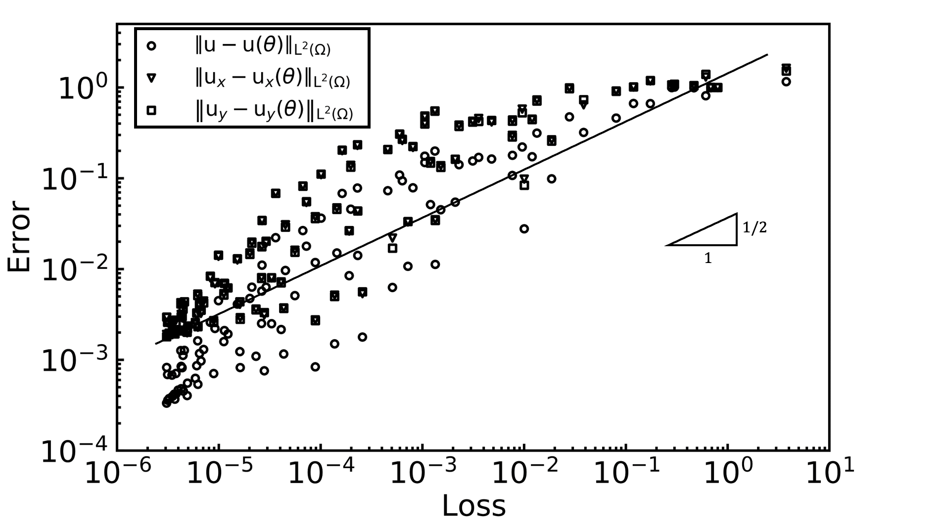
Figure 7: 2D Allen–Cahn equation: The evolution of $l^{2}$ solution errors for $u$, $u_{x}$ and $u_{y}$ as a function of the training loss value using Residuals-RAE.

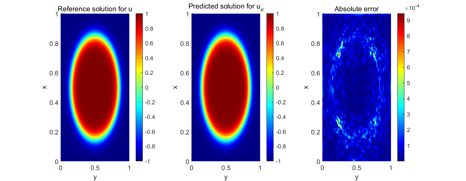
(a) Results for 2D Allen–Cahn equation ($t=0$) using Residuals-RAE PINNs.

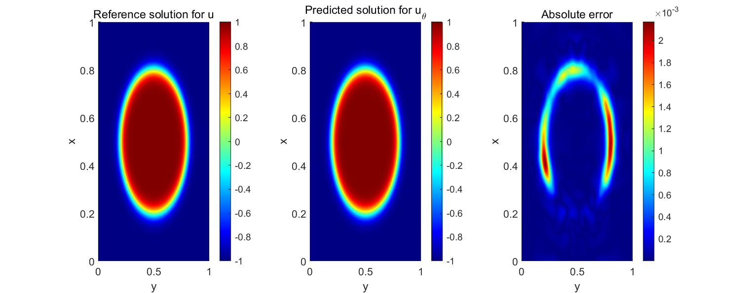
(b) Results for 2D Allen–Cahn ($t=2.5$) equation using Residuals-RAE PINNs.

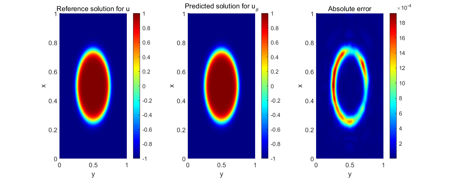
(c) Results for 2D Allen–Cahn equation ($t=5.0$) using Residuals-RAE PINNs.

Figure 8: Results for solving 2D Allen–Cahn equation using Residuals-RAE. $1^{st}$ column: Reference $u$, $2^{nd}$ column: the predicted $u$ from Residuals-RAE, $3^{rd}$ column: absolute pointwise error (relative $L^{2}$ error: $6.42e-04$) at different time snapshots (a) t=0, (b) t=2.5, (c) t=5.

4 Physics Informed Neural Networks for Approximating the Cahn–Hilliard Equation

4.1 Cahn–Hilliard Equation

We first review the general form of Cahn–Hilliard equation in the domain $\Omega:=D\times(0,T]$, where $D\subset\mathbb{R}^{d}$ and $d\in\mathbb{N}$. The equation can be represented as follows:

$$u_{t}-\nabla^{2}\left(\kappa f(u)-(\alpha\kappa)\nabla^{2}u(\bm{x},t)\right)=0,\quad t\in(0,T],\quad\bm{x}\in D$$ (4.1a)

$$u(\bm{x},0)=\psi(\bm{x}),\quad\bm{x}\in D$$ (4.1b)

$$u(\bm{x},t)=u(-\bm{x},t),\quad t\in(0,T],\quad\bm{x}\in\partial D$$ (4.1c)

$$\nabla u(\bm{x},t)=\nabla u(-\bm{x},t),\quad t\in(0,T],\quad\bm{x}\in\partial D$$ (4.1d)

where the coefficients $\kappa$ and $\alpha$ are non-negative constants. The nonlinear term $f(u)$ is a polynomial of degree 3 with positive dominant coefficient. $\psi$ as the initial distribution for $u$ belongs to $L^{q}(D)\cap C(D)$ for $q\geq 4$. The boundary conditions are assumed to be periodic.

Lemma 4.1

([47]) There exists a unique weak solution $u(t,x)$ for the Cahn–Hilliard equation (4.1), where $t\in(0,T]$ and $x\in D$, in the space $L^{\infty}\left((0,T],L^{q}(D)\right)$ .

Lemma 4.2

Let $k\in\mathbb{N}$, $\psi\in H^{r}(D)$ and $f\in C^{r}(\mathbb{R})$ with $r>\frac{d}{2}+k$, then there exists $T>0$ and a weak solution $u$ to Cahn–Hilliard equation (4.1) such that $u$ satisfies $u(t=0)=\psi$, $u\in C^{k}((0,T]\times D)$ and $\partial_{t}u\in C^{k-1}((0,T]\times D)$.

The proof of Lemma 4.2 closely resembles the proof in Lemma 3.2.

4.2 Physics Informed Neural Networks

In order to solve the equation mentioned above, we can utilize a neural network denoted as $u_{\theta}:\Omega\rightarrow\mathbb{R}$, where $\Omega:=D\times(0,T]$ and is parameterized by $\theta$. Then, we can have the residuals:

$$R_{\text{int }}^{CH}\left[u_{\theta}\right](\bm{x},t)=\partial_{t}u_{\theta}-\nabla^{2}(-(\alpha\kappa)\nabla^{2}u_{\theta}+\kappa f(u_{\theta})),$$ (4.2a)

$$R_{tb}^{CH}\left[u_{\theta}\right](\bm{x})=u_{\theta}(\bm{x},0)-\psi(\bm{x}),$$ (4.2b)

$$R_{sb1}^{CH}\left[u_{\theta}\right](\bm{x},t)=u_{\theta}(\bm{x},t)-u_{\theta}(-\bm{x},t),$$ (4.2c)

$$R_{sb2}^{CH}\left[u_{\theta}\right](\bm{x},t)=\nabla u_{\theta}(\bm{x},t)-\nabla u_{\theta}(-\bm{x},t).$$ (4.2d)

The generalization error, denoted as $\mathcal{E}_{G}^{CH}(\theta)^{2}$, is defined as follows:

$$\mathcal{E}_{G}^{CH}(\theta)^{2} =\int_{D}|R_{tb}^{CH}|^{2}d\bm{x}+\int_{0}^{T}\int_{D}|R_{int}^{CH}|^{2}d\bm{x}dt$$ (4.3)

$$+2(\alpha\kappa)\hat{M}(\int_{0}^{T}\int_{\partial{D}}|{R_{sb1}^{CH}}|^{2}ds(\bm{x})dt)^{1/2}+(\int_{0}^{T}\int_{\partial{D}}|{\Delta R_{sb1}^{CH}}|^{2}ds(\bm{x})dt)^{1/2}$$

$$+(\int_{0}^{T}\int_{\partial{D}}|{R_{sb2}^{CH}}|^{2}ds(\bm{x})dt)^{1/2}+(\int_{0}^{T}\int_{\partial{D}}|{\Delta{R}_{sb2}^{CH}|^{2}ds(\bm{x})}dt)^{1/2}),$$

where $\hat{M}=|\partial{D}|^{1/2}\cdot(\|{u}\|_{C^{3}(\partial{D}\times\left(0,T\right])}+\|{u_{\theta}}\|_{C^{3}(\partial{D}\times\left(0,T\right])})$ . Let $\mathcal{S}^{CH}=\mathcal{S}^{CH}_{int}\cup\mathcal{S}^{CH}_{tb}\cup\mathcal{S}^{CH}_{sb}$ be the set of training points based on appropriate numerical quadrature rules of (4.3), where $\mathcal{S}^{CH}_{int}=\{(\bm{x}_{int}^{(i)},t_{int}^{(i)})\}_{i=1}^{N_{int}}$, $\mathcal{S}^{CH}_{tb}=\{(\bm{x}_{tb}^{(i)})\}_{i=1}^{N_{tb}}$, $\mathcal{S}^{CH}_{sb}=\{(\bm{x}_{sb}^{(i)},t_{sb}^{(i)})\}_{i=1}^{N_{sb}}$ correspond to control equation, initial, and boundary conditions, respectively. Then we define the training error $\mathcal{E}_{T}^{CH}(\theta,\mathcal{S})^{2}$ to estiamte the generalization error as follow,

$$\mathcal{E}_{T}^{CH}(\theta,\mathcal{S})^{2} =\sum_{i=1}^{N_{tb}}\lambda^{(i)}_{tb}|R_{tb}^{CH}(\bm{x}_{tb}^{(i)})|^{2}+\sum_{i=1}^{N_{int}}\lambda^{(i)}_{int}|R_{int}^{CH}(\bm{x}_{int}^{(i)},t_{int}^{(i)})|^{2}$$ (4.4)

$$+2(\alpha\kappa)\hat{M}((\sum_{i=1}^{N_{sb}}\lambda^{(i)}_{sb}|R_{sb1}^{CH}(\bm{x}_{sb}^{(i)},t_{sb}^{(i)})|^{2})^{1/2}+(\sum_{i=1}^{N_{sb}}\lambda^{(i)}_{sb}|\Delta R_{sb1}^{CH}(\bm{x}_{sb}^{(i)},t_{sb}^{(i)})|^{2})^{1/2}$$

$$\quad\quad\quad\quad+(\sum_{i=1}^{N_{sb}}\lambda^{(i)}_{sb}|R_{sb2}^{CH}(\bm{x}_{sb}^{(i)},t_{sb}^{(i)})|^{2})^{1/2}+(\sum_{i=1}^{N_{sb}}\lambda^{(i)}_{sb}|\Delta R_{sb2}^{CH}(\bm{x}_{sb}^{(i)},t_{sb}^{(i)})|^{2})^{1/2}).$$

Additionally, by defining $\hat{u}=u_{\theta}-u$, we can also define the total error $\mathcal{E}^{CH}(\theta)^{2}$ as follows:

$$\mathcal{E}(\theta)^{2}=||\hat{u}(\bm{x},t)||^{2}_{L^{2}(D\times(0,T])}+2\alpha\kappa\int_{0}^{T}||\Delta\hat{u}(\bm{x},t)||^{2}_{L^{2}(D\times(0,t])}dt.$$ (4.5)

4.3 Error Analysis

In this subsection, we will present a summary of the results obtained from the PINN approximations to the Cahn–Hilliard equations. These results are outlined in the following theorems.

To begin with, considering the Cahn–Hilliard equations and the corresponding definitions for various residuals, we have

$$R_{\text{int }}^{CH}(\bm{x},t)=\partial_{t}\hat{u}-\nabla^{2}(-(\alpha\kappa)\nabla^{2}\hat{u}+\kappa(f(u_{\theta})-f(u))),$$ (4.6a)

$$R_{tb}^{CH}(\bm{x})=\hat{u}(\bm{x},0),$$ (4.6b)

$$R_{sb1}^{CH}(\bm{x},t)=\hat{u}(\bm{x},t)-\hat{u}(-\bm{x},t),$$ (4.6c)

$$R_{sb2}^{CH}(\bm{x},t)=\nabla\hat{u}(\bm{x},t)-\nabla\hat{u}(-\bm{x},t),$$ (4.6d)

where $\hat{u}=u_{\theta}-u$ is substituted into (4.2) to obtain the above equations.

4.3.1 Bound on the Residuals

Lemma 2.1 elucidates that a tanh neural network with two hidden layers is capable of reducing $\|\hat{u}\|_{H^{2}(D\times(0,T])}$ to an arbitrarily small value. Furthermore, the lemma provides a specific limit for this estimation. Consequently, using this Lemma, we are able to demonstrate the existence of an upper bound for the residuals of Cahn–Hilliard equations. Subsequently, we present the findings related to the application of the Physics-Informed Neural Network (PINN) to the Cahn–Hilliard equation, which are elaborated below.

Theorem 4.1

Let $d,r,k\in\mathbb{N}$ with $k\geq 5$. Let $\psi\in H^{r}(D)$ and $f\in C^{k-1}\left((0,T];H^{r-1}(D)\right)$ where $r>\frac{d}{2}+k$. For every integer $N>5$, there exists a tanh neural network $u_{\theta}$ with two hidden layers, of widths at most $3\left\lceil\frac{k+n-2}{2}\right\rceil\left|P_{k-1,d+2}\right|+\lceil NT\rceil+d(N-1)$, such that

$$\left\|R_{int}^{CH}\right\|_{L^{2}(\Omega)}\lesssim\ln^{2}\left(N\right)N^{-k+4},$$ (4.7a)

$$\left\|R_{sb2}^{CH}\right\|_{L^{2}(\partial D\times(0,T])}\lesssim\ln^{2}\left(N\right)N^{-k+2},$$ (4.7b)

$$\left\|R_{sb1}^{CH}\right\|_{L^{2}(\partial D\times(0,T])},\left\|R_{\text{tb }}^{CH}\right\|_{L^{2}(D)}\lesssim\ln\left(N\right)N^{-k+1}.$$ (4.7c)

The proof for Theorem 4.1 is provided in the Appendix C.

In light of the established bounds (4.7), it becomes evident that selecting a sufficiently large number of $N$, we can effectively minimize both the residuals of the Physics-Informed Neural Network (PINN) as stated in equation (4.6), and reduce the generalization error to extremely small levels. This observation is crucial in illustrating the capacity of PINNs to adapt and converge effectively in response to the complexity of the network configuration.

We next demonstrate that the total error remains minimal when the generalization error $\mathcal{E}_{G}(\theta)^{2}$ is small using the PINN approximation.

Theorem 4.2

Let $d\in\mathbb{N},u\in C^{1}(\Omega)$ be the classical solution to the Cahn–Hilliard equations. Let $u_{\theta}$ denote the PINN approximation with parameter $\theta$. Then the following relation holds,

$$\mathcal{E}(\theta)^{2}=||\hat{u}(\bm{x},t)||^{2}_{L^{2}(D\times(0,T])}+2\alpha\kappa\int_{0}^{T}||\Delta\hat{u}(\bm{x},t)||^{2}_{L^{2}(D\times(0,t])}dt\leq C_{G}T\exp((1+2\kappa{M})T),$$ (4.8)

where

$$C_{G}=\int_{D}|R_{tb}|^{2}d\bm{x}+\int_{0}^{T}\int_{D}|R_{int}|^{2}d\bm{x}dt+2(\alpha\kappa)\hat{M}\hat{C},$$

and M is a Lipschitz constant of $$\nabla^{2}{f} \hat{M}=|\partial{D}|^{1/2}\cdot(\|{u}\|_{C^{3}(\partial{D}\times\left(0,T\right])}+\|{u_{\theta}}\|_{C^{3}(\partial{D}\times\left(0,T\right])}) \hat{C}=(\int_{0}^{T}\int_{\partial{D}}|\Delta{R_{sb1}}|^{2}ds(\bm{x})dt)^{1/2}+(\int_{0}^{T}\int_{\partial{D}}|{R_{sb2}}|^{2}ds(\bm{x})dt)^{1/2}+(\int_{0}^{T}\int_{\partial{D}}|{R_{sb1}}|^{2}ds(\bm{x})dt)^{1/2}+(\int_{0}^{T}\int_{\partial{D}}|{\Delta{R}_{sb2}|^{2}ds(\bm{x})}dt)^{1/2}.$$, ,

The proof for Theorem 4.2 is provided in the Appendix C.

The upcoming theorem will further substantiate the idea that the total error is essentially determined and limited by the training error and the size of the training set.

Theorem 4.3

Let $d\in\mathbb{N}$ and $T>0$. Let $u\in C^{4}(\Omega=D\times(0,T])$ be the classical solution of the Cahn–Hilliard equations, and let $u_{\theta}$ represent the PINN approximation with parameter $\theta$. Then the total error can be bounded as follows:

$$\mathcal{E}(\theta)^{2} =||\hat{u}(\bm{x},t)||^{2}_{L^{2}(D\times(0,T])}+2\alpha\kappa\int_{0}^{T}||\Delta\hat{u}(\bm{x},t)||^{2}_{L^{2}(D\times(0,t])}dt$$ (4.9)

$$\leq C_{T}T\exp((1+2\kappa{M})T)=\mathcal{O}(\mathcal{E}^{CH}_{T}(\theta,\mathcal{S}^{CH})^{2}+M_{tb}^{-\frac{2}{d}}+M_{int}^{-\frac{2}{d+1}}+M_{sb}^{-\frac{2}{d}}).$$

The constant $C_{T}$ is defined as

$$C_{T}= C_{\left[{(R_{tb}^{CH})}^{2}\right]}M_{tb}^{-\frac{2}{d}}+\mathcal{Q}_{M_{tb}}^{D}\left[{(R_{tb}^{CH})}^{2}\right]+C_{\left[{(R_{int}^{CH})}^{2}\right]}M_{int}^{-\frac{2}{d+1}}+\mathcal{Q}_{M_{int}}^{\Omega}\left[{(R_{int}^{CH})}^{2}\right]$$

$$+2(\alpha\kappa)\hat{M}(C_{[\left(R_{sb1}^{CH})^{2}\right]}M_{sb}^{-\frac{2}{d}}+\mathcal{Q}_{M_{sb}}^{\partial{D}\times\left(0,T\right]}[\left(R_{sb1}^{CH})^{2}\right])^{1/2}$$

$$+2(\alpha\kappa)\hat{M}(C_{[\left(R_{sb2}^{CH})^{2}\right]}M_{sb}^{-\frac{2}{d}}+\mathcal{Q}_{M_{sb}}^{\partial{D}\times\left(0,T\right]}[\left(R_{sb2}^{CH})^{2}\right])^{1/2}$$

$$+2(\alpha\kappa)\hat{M}(C_{[\left(\Delta R_{sb1}^{CH})^{2}\right]}M_{sb}^{-\frac{2}{d}}+\mathcal{Q}_{M_{sb}}^{\partial{D}\times\left(0,T\right]}[\left(\Delta R_{sb1}^{CH})^{2}\right])^{1/2}$$

$$+2(\alpha\kappa)\hat{M}(C_{[\left(\Delta R_{sb2}^{CH})^{2}\right]}M_{sb}^{-\frac{2}{d}}+\mathcal{Q}_{M_{sb}}^{\partial{D}\times\left(0,T\right]}[\left(\Delta R_{sb2}^{CH})^{2}\right])^{1/2}$$

and $\hat{M}=|\partial{D}|^{1/2}\cdot(\|{u}\|_{C^{3}(\partial{D}\times\left(0,T\right])}+\|{u_{\theta}}\|_{C^{3}(\partial{D}\times\left(0,T\right])})$.

The proof for Theorem 4.3 is provided in the Appendix C.

Here, we also want to emphasize that the Cahn–Hilliard equation includes high-order derivatives. To simplify it, a commonly used method is to decompose it into two coupled second-order partial differential equations, as shown below:

$$u_{t}-\nabla^{2}(-(\alpha\kappa)\mu+\kappa f(u))=0,\quad\mu=\nabla^{2}u\quad t\in(0,T],\quad x\in D\subset\mathbb{R}^{D}$$ (4.10a)

$$f(u)=u^{3}-u.$$ (4.10b)

The decomposition presented here is similar to the second-order decomposition employed in the work conducted by Qian et al [29]. for general second-order PDEs in the temporal domain. Qian et al. divided the residual loss, which is determined by the interior points of second-order PDEs, into two components. By utilizing the error analysis theorem derived earlier in the above Cahn–Hilliard equation (4.1), a new approximation for the error in Cahn–Hilliard equations can be derived. To begin with, we reformulate the residuals (4.6) using the following definition of residuals,

$$R_{int1}=\hat{\mu}-\nabla^{2}\hat{u},$$ (4.11a)

$$R_{int2}=\hat{u}_{t}+\alpha\kappa\nabla^{2}\hat{\mu}-\kappa\nabla^{2}(f(u_{\theta})-f(u)),$$ (4.11b)

$$R_{tb}=\hat{u}(x,0),$$ (4.11c)

$$R_{sb1}=\hat{u}(x,t)-\hat{u}(-x,t),$$ (4.11d)

$$R_{sb2}=\nabla\hat{u}(x,t)-\nabla\hat{u}(-x,t)$$ (4.11e)

We next redefine the generalization error as $\mathcal{E}_{G}^{CH}(\theta)^{2}$, which is expressed as follows:

$$\mathcal{E}_{G}^{CH}(\theta)^{2} =\int_{D}|R_{tb}^{CH}|^{2}d\bm{x}+\int_{0}^{T}\int_{D}|R_{int2}^{CH}|^{2}d\bm{x}dt+(\alpha\kappa)\int_{0}^{T}\int_{D}|R_{int1}^{CH}|^{2}d\bm{x}dt$$ (4.12)

$$+2(\alpha\kappa)\hat{M}(\int_{0}^{T}\int_{\partial{D}}|{R_{sb1}^{CH}}|^{2}ds(\bm{x})dt)^{1/2}+(\int_{0}^{T}\int_{\partial{D}}|{\Delta R_{sb1}^{CH}}|^{2}ds(\bm{x})dt)^{1/2}$$

$$+(\int_{0}^{T}\int_{\partial{D}}|{R_{sb2}^{CH}}|^{2}ds(\bm{x})dt)^{1/2}+(\int_{0}^{T}\int_{\partial{D}}|{\Delta{R}_{sb2}^{CH}|^{2}ds(\bm{x})}dt)^{1/2}),$$

where $\hat{M}=\max\{M_{u},M_{\mu}\}$, and $M_{u}=|\partial{D}|^{1/2}\cdot(\|u\|_{C^{1}(\partial{D}\times\left(0,T\right])}+\|u_{\theta}\|_{C^{1}(\partial{D}\times\left(0,T\right])})$ $M_{\mu}=|\partial{D}|^{1/2}\cdot(\|\mu\|_{C^{1}(\partial{D}\times\left(0,T\right])}+\|\mu_{\theta}\|_{C^{1}(\partial{D}\times\left(0,T\right])})$.

Since it is not feasible to directly minimize the generalization error $\mathcal{E}_{G}^{(CH)}(\theta)^{2}$ in practice, we approximate the integrals in (4.12) using numerical quadrature. Therefore, we define the training error as follows,

$$\mathcal{E}_{T}^{CH}(\theta,\mathcal{S})^{2} =\sum_{i=1}^{N_{tb}}\lambda^{(i)}_{tb}|R_{tb}^{CH}(\bm{x}_{tb}^{(i)})|^{2}+\sum_{i=1}^{N_{int}}\lambda^{(i)}_{int}|R_{int2}^{CH}(\bm{x}_{int}^{(i)},t_{int}^{(i)})|^{2}+(\alpha\kappa)\sum_{i=1}^{N_{int}}\lambda^{(i)}_{int}|R_{int1}^{CH}(\bm{x}_{int}^{(i)},t_{int}^{(i)})|^{2}$$ (4.13)

$$+2(\alpha\kappa)\hat{M}((\sum_{i=1}^{N_{sb}}\lambda^{(i)}_{sb}|R_{sb1}^{CH}(\bm{x}_{sb}^{(i)},t_{sb}^{(i)})|^{2})^{1/2}+(\sum_{i=1}^{N_{sb}}\lambda^{(i)}_{sb}|\Delta R_{sb1}^{CH}(\bm{x}_{sb}^{(i)},t_{sb}^{(i)})|^{2})^{1/2}$$

$$\quad\quad\quad\quad+(\sum_{i=1}^{N_{sb}}\lambda^{(i)}_{sb}|R_{sb2}^{CH}(\bm{x}_{sb}^{(i)},t_{sb}^{(i)})|^{2})^{1/2}+(\sum_{i=1}^{N_{sb}}\lambda^{(i)}_{sb}|\Delta R_{sb2}^{CH}(\bm{x}_{sb}^{(i)},t_{sb}^{(i)})|^{2})^{1/2}).$$

Here, $\mathcal{S}^{CH}=\mathcal{S}^{CH}_{int}\cup\mathcal{S}^{CH}_{tb}\cup\mathcal{S}^{CH}_{sb}$ represents the collection of training points. Specifically, $\mathcal{S}^{CH}_{int}=\{(\bm{x}_{int}^{(i)},t_{int}^{(i)})\}_{i=1}^{N_{int}}$ , $\mathcal{S}^{CH}_{tb}=\{(\bm{x}_{tb}^{(i)})\}_{i=1}^{N_{tb}}$ , $\mathcal{S}^{CH}_{sb}=\{(\bm{x}_{sb}^{(i)},t_{sb}^{(i)})\}_{i=1}^{N_{sb}}$ correspond to the control equation, initial conditions, and boundary conditions, respectively. Additionally, we can define the total error $\mathcal{E}^{CH}(\theta)^{2}$ by introducing the variable $\hat{u}=u_{\theta}-u$. This can be expressed as follows:

$$\mathcal{E}(\theta)^{2}=||\hat{u}(\bm{x},t)||^{2}_{L^{2}(D\times(0,T])}+\alpha\kappa\int_{0}^{T}||\Delta\hat{u}(\bm{x},t)||^{2}_{L^{2}(D\times(0,t])}dt.$$ (4.14)

The forthcoming theorem aims to perform an error analysis on the decoupled Cahn–Hilliard (CH) equation. It will adopt a methodology similar to the one used in Theorems 4.1, 4.2, and 4.3. This approach entails estimating the residuals and total error associated with the CH equation, with the objective of obtaining conclusions that are consistent with those derived in the previous theorems.

Theorem 4.4

Let $d,r,k\in\mathbb{N}$ with $k\geq 5$. Let $\psi\in H^{r}(D)$ and $f\in C^{k-1}\left((0,T];H^{r-1}(D)\right)$ with $r>\frac{d}{2}+k$. For every integer $N>5$, there are tanh neural networks $u_{\theta}$ and $\mu_{\theta}$, each with two hidden layers, where the widths are at most $3\left\lceil\frac{k+n-2}{2}\right\rceil\left|P_{k-1,d+2}\right|+\lceil NT\rceil+d(N-1)$, such that

$$\left\|R_{int1}^{CH}\right\|_{L^{2}(\Omega)}\lesssim\ln^{2}\left(N\right)N^{-k+2},$$ (4.15a)

$$\left\|R_{int2}^{CH}\right\|_{L^{2}(\Omega)}\lesssim\ln^{2}(N)N^{-k+4},$$ (4.15b)

$$\left\|R_{sb2}^{CH}\right\|_{L^{2}(\partial D\times(0,T])}\lesssim\ln^{2}(N)N^{-k+2},$$ (4.15c)

$$\left\|R_{sb1}^{CH}\right\|_{L^{2}(\partial D\times(0,T])},\left\|R_{tb}^{CH}\right\|_{L^{2}(D)}\lesssim\ln(N)N^{-k+1}.$$ (4.15d)

In contrast to Theorem 4.1, the addition of $\mu=\nabla^{2}u$ introduces an additional factor in the estimation of the residual. Consequently, the calculation for the upper bound of the residual varies slightly from that of Theorem 4.1. Nevertheless, the overall conclusion remains unchanged.

Theorem 4.5

Let $d\in\mathbb{N},u\in C^{1}(\Omega)$ and $\mu\in C^{1}(\Omega)$ be the classical solution to the Cahn–Hilliard equations. Let $u_{\theta}$ and $\mu_{\theta}$ denote the PINN approximation with parameter $\theta$. Then the following relation holds,

$$\mathcal{E}(\theta)^{2}=\|\hat{u}(\bm{x},t)\|_{L^{2}(D\times(0,T])}^{2}+\alpha\kappa\int_{0}^{T}\|\hat{\mu}(\bm{x},t)\|_{L^{2}(D\times(0,t])}^{2}dt\leq C_{G}T\exp((1+2\kappa{M})T),$$ (4.16)

where

$$C_{G}=\int_{D}|R_{tb}|^{2}d\bm{x}+\int_{0}^{T}\int_{D}|R_{int2}|^{2}d\bm{x}dt+(\alpha\kappa)\int_{0}^{T}\int_{D}|R_{int1}|^{2}d\bm{x}dt+2(\alpha\kappa)\hat{M}\hat{C},$$

and $\hat{M}=\max\{M_{u},M_{\mu}\}$, $M_{u}=|\partial{D}|^{1/2}\cdot(\|u\|_{C^{1}(\partial{D}\times\left(0,T\right])}+\|u_{\theta}\|_{C^{1}(\partial{D}\times\left(0,T\right])})$ $M_{\mu}=|\partial{D}|^{1/2}\cdot(\|\mu\|_{C^{1}(\partial{D}\times\left(0,T\right])}+\|\mu_{\theta}\|_{C^{1}(\partial{D}\times\left(0,T\right])})$, $\hat{C}=(\int_{0}^{T}\int_{\partial{D}}|\Delta{R_{sb1}}|^{2}ds(\bm{x})dt)^{1/2}+(\int_{0}^{T}\int_{\partial{D}}|{R_{sb2}}|^{2}ds(\bm{x})dt)^{1/2}+(\int_{0}^{T}\int_{\partial{D}}|{R_{sb1}}|^{2}ds(\bm{x})dt)^{1/2}+(\int_{0}^{T}\int_{\partial{D}}|{\Delta{R}_{sb2}|^{2}ds(\bm{x})}dt)^{1/2}.$

The definition of total error in Theorem 4.5 differs subtly from that in Theorem 4.2, mainly because of the inclusion of the term $\mu=\nabla^{2}u$. Despite these discrepancies in definition, the ultimate results of both theorems are similar. In other words, both Theorem 4.5 and Theorem 4.2 suggest that the total error can be controlled by considering the residual terms and that there exists an explicit upper limit for this error. This implies that, despite differences in how equations and variables are handled, Theorem 4.5 aligns with the foundational theoretical framework of Theorem 4.2: by accurately estimating the residual terms, one can effectively control the total error in the model when dealing with specific issues.

According to Theorem 4.5 regarding the representation of total error, Theorem 4.6 demonstrates that by minimizing the training error and utilizing a sufficiently large training set, it is possible to reduce the total error to a negligible level.

Theorem 4.6

Let $d\in\mathbb{N}$ and $T>0$. Let $u\in C^{1}((0,T];H^{2}(D))$ and $\mu\in C^{1}((0,T];H^{1}(D))$. $u_{\theta}$ and $\mu_{\theta}$ denote the PINN approximation with parameter $\theta$. Then the total error satisfies

$$\mathcal{E}(\theta)^{2}=\|\hat{u}(\bm{x},t)\|_{L^{2}(D\times(0,T])}^{2}+\alpha\kappa\int_{0}^{T}\|\hat{\mu}(\bm{x},t)\|_{L^{2}(D\times(0,t])}^{2}dt \leq C_{T}T\exp((1+2\kappa{M})T)$$ (4.17)

$$=\mathcal{O}(\mathcal{E}^{CH}_{T}(\theta,\mathcal{S}^{CH})^{2}+M_{tb}^{-\frac{2}{d}}+M_{int}^{-\frac{2}{d+1}}+M_{sb}^{-\frac{2}{d}}).$$

The constant $C_{T}$ is defined as

$$C_{T}= C_{\left[(R_{tb}^{CH})^{2}\right]}M_{tb}^{-\frac{2}{d}}+\mathcal{Q}_{M_{tb}}^{D}[\left(R_{tb}^{CH})^{2}\right]+C_{\left[(R_{int2}^{CH})^{2}\right]}M_{int}^{-\frac{2}{d+1}}+\mathcal{Q}_{M_{int}}^{\Omega}[\left(R_{int2}^{CH})^{2}\right]$$

$$+(\alpha\kappa)(C_{\left[(R_{int1}^{CH})^{2}\right]}M_{int}^{-\frac{2}{d+1}}+\mathcal{Q}_{M_{int}}^{\Omega}\left[(R_{int1}^{CH})^{2}\right])$$

$$+2(\alpha\kappa)\hat{M}(C_{[\left(R_{sb1}^{CH})^{2}\right]}M_{sb}^{-\frac{2}{d}}+\mathcal{Q}_{M_{sb}}^{\partial{D}\times\left(0,T\right]}[\left(R_{sb1}^{CH})^{2}\right])^{1/2}$$

$$+2(\alpha\kappa)\hat{M}(C_{[\left(R_{sb2}^{CH})^{2}\right]}M_{sb}^{-\frac{2}{d}}+\mathcal{Q}_{M_{sb}}^{\partial{D}\times\left(0,T\right]}[\left(R_{sb2}^{CH})^{2}\right])^{1/2}$$

$$+2(\alpha\kappa)\hat{M}(C_{[\left(\Delta R_{sb1}^{CH})^{2}\right]}M_{sb}^{-\frac{2}{d}}+\mathcal{Q}_{M_{sb}}^{\partial{D}\times\left(0,T\right]}[\left(\Delta R_{sb1}^{CH})^{2}\right])^{1/2}$$

$$+2(\alpha\kappa)\hat{M}(C_{[\left(\Delta R_{sb2}^{CH})^{2}\right]}M_{sb}^{-\frac{2}{d}}+\mathcal{Q}_{M_{sb}}^{\partial{D}\times\left(0,T\right]}[\left(\Delta R_{sb2}^{CH})^{2}\right])^{1/2}$$

and $\hat{M}=\max\{M_{u},M_{\mu}\}$, $M_{u}=|\partial{D}|^{1/2}\cdot(\|u\|_{C^{1}(\partial{D}\times\left(0,T\right])}+\|u_{\theta}\|_{C^{1}(\partial{D}\times\left(0,T\right])})$ $M_{\mu}=|\partial{D}|^{1/2}\cdot(\|\mu\|_{C^{1}(\partial{D}\times\left(0,T\right])}+\|\mu_{\theta}\|_{C^{1}(\partial{D}\times\left(0,T\right])})$.

The difference between Theorem 4.3 and Theorem 4.6 lies in the definition of total error. This discrepancy arises from the division of the system into two simply coupled problems, achieved by introducing an auxiliary function $\mu=\nabla^{2}u$. Our analysis reveals that the outcomes of Theorem 4.6 are similar to those of Theorem 4.3. Specifically, the total error can be controlled by the training error and the size of the sample set.

4.4 Numerical Examples

4.4.1 1D Cahn–Hilliard equation

We will first examine the performance of the 1D Cahn–Hilliard equation, which describes the process of phase separation and interface development. The spatial-temporal domain is taken as $(x,t)\in D\times(0,T]=[-1,1]\times(0,0.5]$. Then the equation is given by:

$$u_{t}-\left(\kappa\left(u^{3}-u\right)-\alpha\kappa u_{xx}\right)_{xx}=0,\qquad(x,t)\in[-1,1]\times(0,0.5]$$ (4.18a)

$$u(x,0)=-\cos(2\pi x),\qquad(x,t)\in[-1,1]\times\{0\}$$ (4.18b)

$$u(-x,t)=u(x,t),\qquad(x,t)\in\partial D\times(0,0.5]$$ (4.18c)

$$\nabla u(-x,t)=\nabla u(x,t),\qquad(x,t)\in\partial D\times(0,0.5]$$ (4.18d)

where the parameter $\kappa=1$ serves as the mobility parameter, influencing the rate of diffusion of components, while the parameter $\alpha=0.02$ is associated with the surface tension at the interface. To implement the Residuals-RAE-PINN scheme for the 1D Cahn–Hilliard equation, we first have the following modified loss function

$$\mathcal{L}(\theta) =\gamma_{int}\cdot\mathcal{L}_{int}(\theta)+\gamma_{tb}\cdot\mathcal{L}_{tb}(\theta)+\gamma_{sb}\cdot\mathcal{L}_{sb}(\theta)$$

$$=\gamma_{int}\cdot\frac{1}{N_{int}}\sum_{i=1}^{N_{int}}\hat{\lambda}_{int}^{(i)}\left|u_{t}(x_{int}^{(i)},t_{int}^{(i)})-\left(\kappa\left(u(x_{int}^{(i)},t_{int}^{(i)})^{3}-u(x_{int}^{(i)},t_{int}^{(i)})\right)-\alpha\kappa u(x_{int}^{(i)},t_{int}^{(i)})_{xx}\right)_{xx}\right|^{2}$$

$$+\gamma_{tb}\cdot\frac{1}{N_{tb}}\sum_{i=1}^{N_{tb}}\left|u(x_{tb}^{(i)},0)-u_{0}(x_{tb}^{(i)})\right|^{2}$$

$$+\gamma_{sb}\cdot\frac{1}{N_{sb}}\sum_{i=1}^{N_{sb}}(\left|u(-x_{sb}^{(i)},t_{sb}^{(i)})-u(x_{sb}^{(i)},t_{sb}^{(i)})\right|^{2}+\left|\nabla u(-x_{sb}^{(i)},t_{sb}^{(i)})-\nabla u(x_{sb}^{(i)},t_{sb}^{(i)})\right|^{2}).$$ (4.19)

For solving the 1D Cahn–Hilliard equation, we assign the weights for different loss terms at $\gamma_{int}=1,\gamma_{sb}=1,\gamma_{tb}=100$. Furthermore, we incorporate a Residuals-RAE weighting scheme for the pointwise weights of residual points, denoted by $\hat{\lambda}_{int}^{(i)}$. The impact of the nearest points on these weights is controlled by the hyper-parameter $k_{int}$, which is set to a value of 50. This parameter plays a pivotal role in determining the extent to which neighboring points influence the calculation of pointwise weights. In this case, we use the training points set $\{(x_{int}^{(i)},t_{int}^{(i)})\}$, $\{(-1,t_{sb}^{(i)})\}$, $\{(x_{tb}^{(i)})\}$ obtained from the Latin hypercube sampling approach. Specifically, we have $N_{int}=10,000$ training points for the residual, $N_{sb}=256$ points for the boundary conditions, and $N_{tb}=512$ points for the initial conditions.

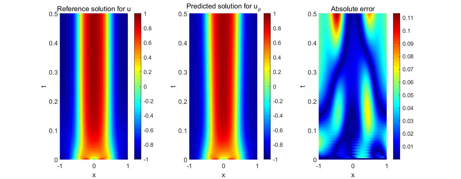
(a) Results for 1D Cahn–Hilliard equation using Residuals-RAE PINNs (with 200 neurons per layer).

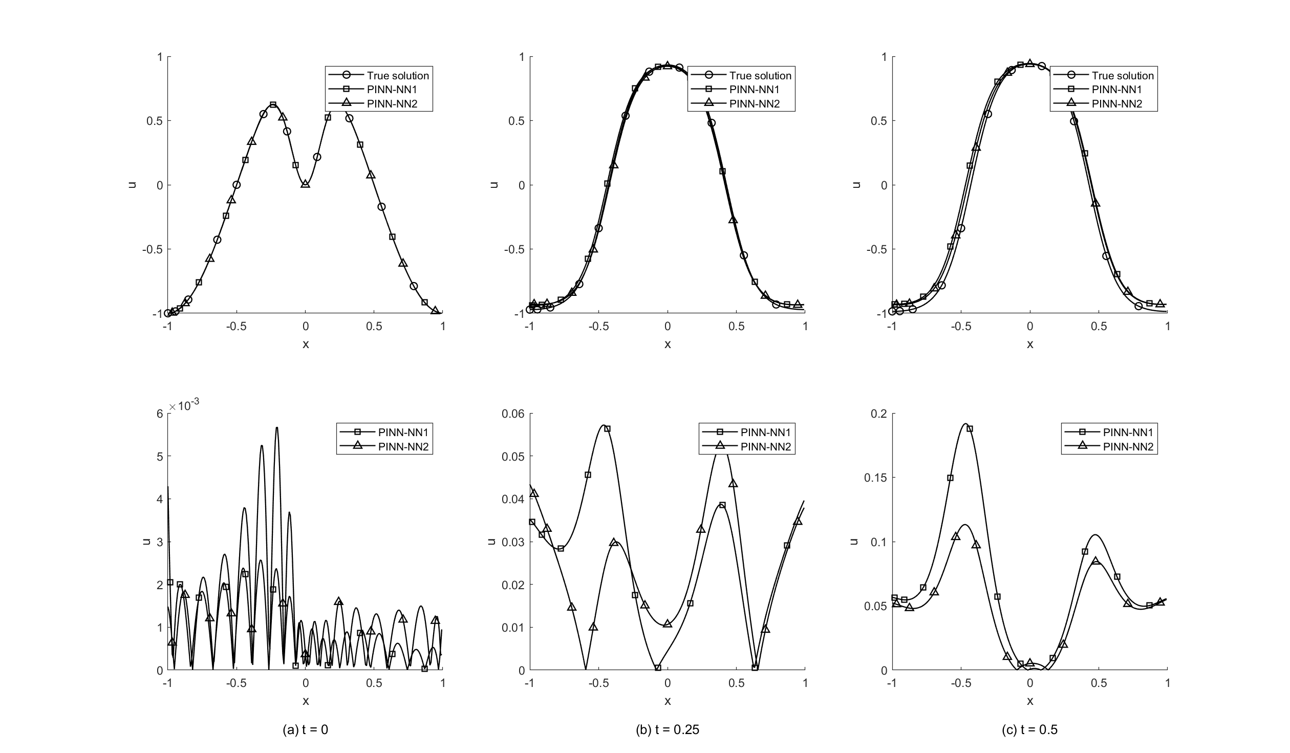
(b) Reference and Residuals-RAE-PINN predicted solutions (neurons per layer $\#1$ and $\#2$) of the 1D Cahn–Hilliard equation (initial condition $\#$ 2) at different time snapshots (a) $t=0$, (b) $t=0.25$, (c) $t=0.5$.

Figure 9: Results for solving 1D Cahn–Hilliard using Residuals-RAE-PINN.

Table 3: Description of training data for 1D Cahn–Hilliard equation.

$$\begin{array}[]{lll}\hline\cr N_{tb}&\text{ Initial collocation points }&512\\ N_{sb}&\text{ Boundary collocation points }&256\\ N_{int}&\text{ Residual collocation points }&10,000\\ \hline\cr\end{array}$$

The training process utilizes a neural network architecture with two layers, each consisting of 256 nodes. The network is initialized using the Xavier scheme. The optimization of the loss function involves two stages: to begin with, the network undergoes 5,000 iterations using the Adam optimizer, followed by a refinement stage of 1,000 iterations with the L-BFGS algorithm. The training is deemed complete when the reduction in loss between successive epochs is below a certain threshold, specifically less than $10^{-7}$. The effectiveness of this Residuals-RAE method is quantified by the relative $L2$ error, with which yielding errors in the order of $5\times 10^{-2}$. The pointwise error for the results obtained from the PINN at different time snapshots is plotted in Fig. 9(b). It can be observed that the results of PINN-NN1 with 256 neurons and PINN-NN2 512 neurons per layer produce the displayed results.

Fig. 10 illustrates the solution error versus training loss relationship during the solution process of the Cahn–Hilliard equation using a Physics-Informed Neural Network (PINN). The numerical results reveal that overall trend of the total error is approximately proportional to the square root of the training loss. This trend is consistent with the expected theoretical behavior as stated in Theorem 4.3. The fluctuations observed in the middle range of loss values appear to scale with a power slightly greater than 1/2. These fluctuations are believed to be a result of the involvement of higher-order derivatives in the Cahn–Hilliard equation, which can introduce complexities in the training dynamics. Despite these perturbations, the general trend aligns with the theoretical predictions, thereby validating the effectiveness of the approach for solving this intricate partial differential equation.

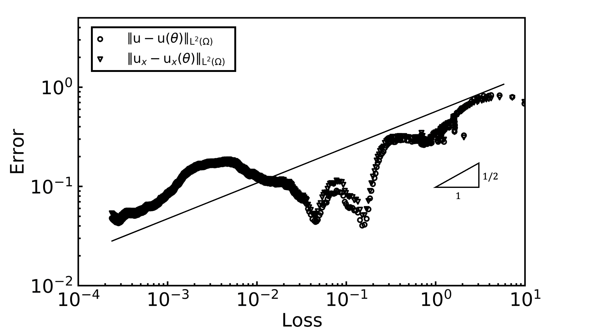
Figure 10: 1D Cahn–Hilliard equation: The dynamics of $l^{2}$ errors of $u$ and $u_{x}$ as a function of the training loss value using Residuals-RAE.

4.4.2 2D Cahn–Hilliard equation

We proceed to evaluate the effectiveness of the Residuals-RAE-PINN algorithm in solving the 2D Cahn–Hilliard equation, as described in [44]. In this study, the authors employ a re-training approach using the same neural network as in previous time segments, similar to the concept of sequence-to-sequence learning [48]. The spatial-temporal domain is taken as $(x,y,t)\in D\times(0,T]=[0,1]^{2}\times(0,0.003]$, and the initial-boundary value problem

$$\partial_{t}u=\kappa\Delta\left(-\alpha^{2}\Delta u+u^{3}-u\right),\qquad(x,y,t)\in D\times(0,T]$$ (4.20a)

$$u(x,y,0)=0.4\cos{(3\pi x)}\cos{(3\pi y)},\qquad(x,y,t)\in D\times(0,T]$$ (4.20b)

$$u^{(d-1)}(x,y,t)=u^{(d-1)}(-x,-y,t),\qquad(x,y,t)\in\partial D\times(0,T]\quad(d=1,2)$$ (4.20c)

where $\kappa=1,\alpha=0.02$. To solve the problem by Residuals-RAE-PINN, we first consider the modified loss function as below

$$\mathcal{L}(\theta) =\gamma_{int}\cdot\mathcal{L}_{int}(\theta)+\gamma_{tb}\cdot\mathcal{L}_{tb}(\theta)+\gamma_{sb}\cdot\mathcal{L}_{sb}(\theta)$$ (4.21)

$$=\gamma_{int}\cdot\frac{1}{N_{int}}\sum_{i=1}^{N_{int}}\hat{\lambda}_{int}^{(i)}\left|u_{t}(x_{int}^{(i)},y_{int}^{(i)},t_{int}^{(i)})+\alpha\kappa\Delta^{2}u(x_{int}^{(i)},y_{int}^{(i)},t_{int}^{(i)})-\kappa\Delta(u^{3}(x_{int}^{(i)},y_{int}^{(i)},t_{int}^{(i)})-u(x_{int}^{(i)},y_{int}^{(i)},t_{int}^{(i)}))\right|^{2}$$

$$+\gamma_{tb}\cdot\frac{1}{N_{tb}}\sum_{i=1}^{N_{tb}}\left|u(x_{tb}^{(i)},y_{tb}^{(i)},0)-0.4\cos{(3\pi x_{tb}^{(i)})\cos{(3\pi y_{tb}^{(i)}})}\right|^{2}$$

$$+\gamma_{sb}\cdot\frac{1}{N_{sb}}\sum_{i=1}^{N_{sb}}\sum_{d=1}^{2}\left|u^{(d-1)}(x_{sb}^{(i)},y_{sb}^{(i)},t_{sb}^{(i)})-u^{(d-1)}(-x_{sb}^{(i)},-y_{sb}^{(i)},t_{sb}^{(i)})\right|^{2},$$

where the weights for the loss terms $\gamma_{int},\gamma_{sb},\gamma_{tb}$, are set to $1,100,100$ respecitively. The input layer of the PINN structure contains 3 neurons, which is the same configuration used for solving the 2D Allen–Cahn equation. The activation function chosen for this neural network is the hyperbolic tangent function ($tanh$).

To generate the collocation points, we randomly sample $N_{int}=10,000,N_{sb}=256,N_{tb}=512$ points from the computational domain using the Latin hypercube sampling technique. In order to obtain pointwise weights, we apply the Residuals-RAE weighting scheme with a hyper-parameter $k_{int}$ set to $50$, controlling the influence of nearby points on the information obtained.

Table 4: Description of training data for 2D Cahn–Hilliard equation.

$$\begin{array}[]{lll}\hline\cr N_{tb}&\text{ Initial collocation points }&512\\ N_{sb}&\text{ Boundary collocation points }&256\\ N_{int}&\text{ Residual collocation points }&10,000\\ \hline\cr\end{array}$$

During the training process, the Xavier-normal method is employed to initialize trainable parameters in the network. To minimize the modified loss function, $50,000$ ADAM and $10,000$ LBFGS iterations are applied. Additionally, the learning rate exponential decay method is employed, with an exponential decay rate of $0.95$ every 5000 epochs in the numerical experiments. It’s important to note that due to the strong non-linearity and higher-order nature of the Cahn–Hilliard equation, accurately capturing the solution with a shallow neural network (e.g. depth = 2) is challenging. As a result, several approaches have been proposed in the field of Physics-Informed Neural Networks (PINNs), such as self-adaptive samples, domain decompositions, and self-adaptive weights. Furthermore, in order to ensure the representability of PINNs, all of these approaches utilize deep or deeper neural networks with multiple layers ($L\geq 5$). From the observation of Fig. 11, it can be seen that the Residuals-RAE-PINN is capable of capturing the solutions for the Cahn–Hilliard equation without requiring domain decomposition in the time dimension, whereas the method proposed in the bc-PINN [44] necessitates it.

To further investigate the relationship between solution errors and the training loss dynamics, we present a log-log plot of $u$, $u_{x}$, and $u_{y}$ in Fig. 12. This type of plot is commonly used in analyzing the training dynamics in previous studies. The reference lines marked with a slope of $1/2$ and $1$ provide a theoretical benchmark for the expected rate of decay of solution errors as the loss decreases. By examining the convergence behavior, we can draw conclusions that the training dynamics is the expected trend.

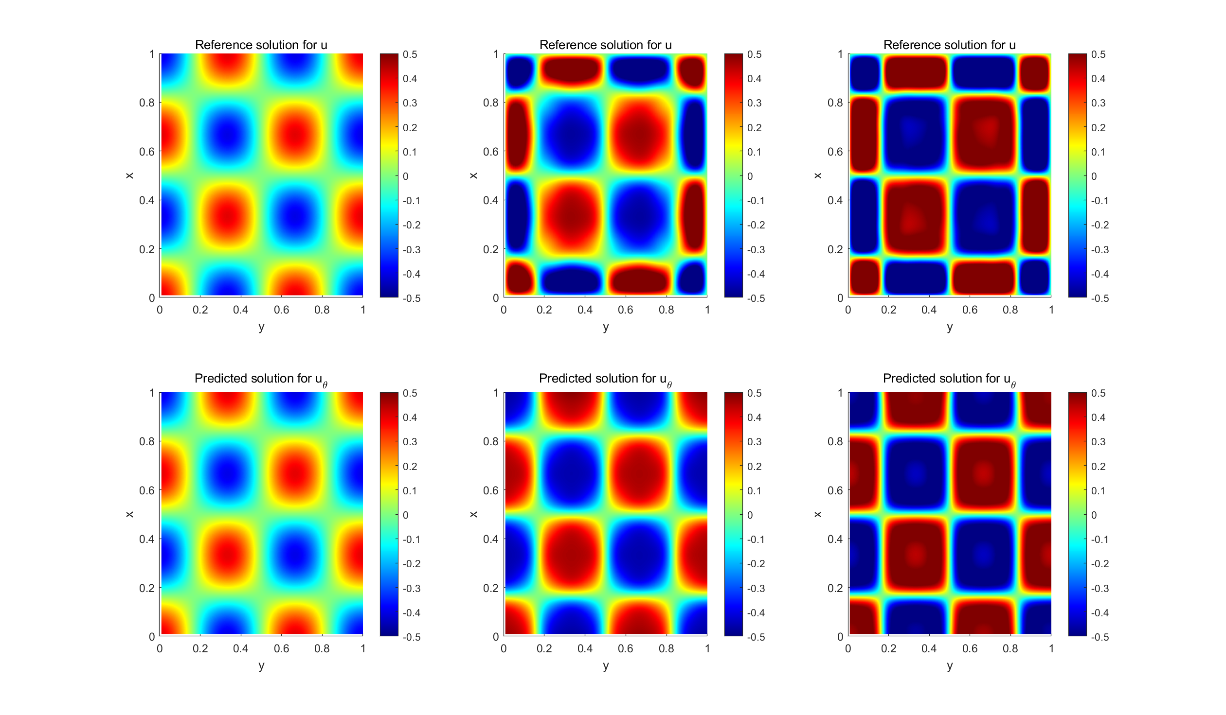
Figure 11: Results for 2D Cahn–Hilliard equation using Residuals-RAE PINNs.

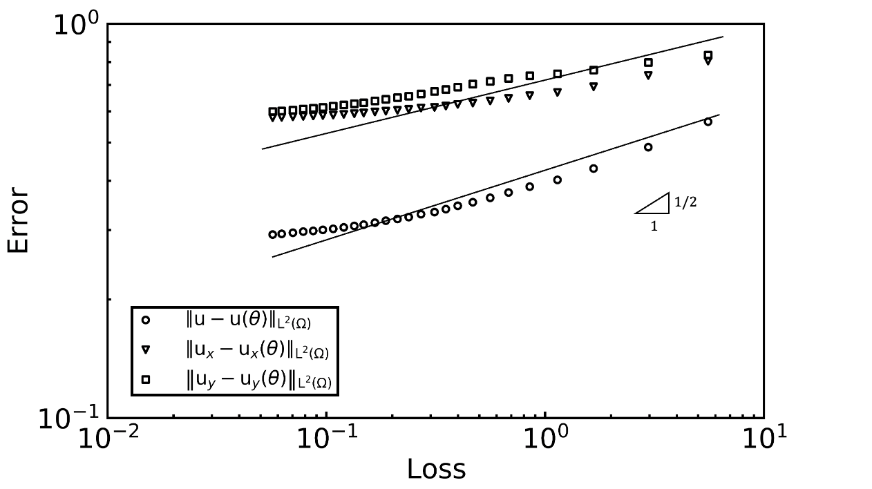
Figure 12: 2D Cahn–Hilliard equation: The dynamics of $l^{2}$ errors of $u$, $u_{x}$ and $u_{y}$ as a function of the training loss value using Residuals-RAE.

5 Conclusion

This paper investigates error estimation when using physics-informed neural networks (PINN) to solve the Allen–Cahn (AC) and Cahn–Hilliard (CH) equations, which are commonly used in phase field modeling research. The primary discoveries are as follows:

• Error bounds are derived for the total error and approximation error between the PINN solution and exact solution for both the AC and CH equations, assuming certain smoothness conditions. These results are presented in Theorem 3.2, Theorem 3.3, Theorem 4.2 and Theorem 4.3.

• For the AC equation, it is shown that the PINN solution converges at a rate of $O(\ln^{2}(N)N^{-k+2})$ as the number of training points $N$ increases, where $k$ represents the continuity of the exact solution in Theorem 3.2 and Theorem 3.3.

• For the CH equation, the PINN solution converges as $N$ increases, as demonstrated in Theorem 4.2 and Theorem 4.3, at a rate of $O(\ln^{2}(N)N^{-k+4})$.

• In our numerical experiment, we employ a pointwise weighting scheme called Residuals-RAE to address the challenge of solving highly nonlinear PDEs in PINNs.

• Numerical results validate the error bounds and convergence rates derived in the theorems.

Overall, the paper offers a comprehensive analysis of the errors involved in utilizing PINNs to approximate solutions for the nonlinear AC and CH equations in phase field modeling. The main contributions lie in the derivation of error bounds and convergence rates for the application of the PINN methodology to these specific problems.

Appendix A Notation

A.1 Basic notation

For $n\in\mathbb{N}$, we denote $\{1,2,\ldots n\}$ by $[n]$ for simplicity in the paper. For two Banach spaces $X,Y,\mathscr{L}(X,Y)$ refers to the set of continuous linear operator mapping from $X$ to $Y$.

For a mapping $f:X\rightarrow Y$, and $u,v\in X,df(u,v)$ denotes Gateaux differential of $f$ at $u$ in the direction of $v$, and $f^{\prime}(u)$ denotes Fréchet derivative of $f$ at $u$.

For $r>0$, and $x_{0}\in X$, where $X$ is a Banach space equipped with norm $\|\cdot\|_{X},B_{int}\left(x_{0}\right)$ refers to $\left\{x\in X:\left\|x-x_{0}\right\|_{X}<r\right\}$.

For a function $f:X\rightarrow\mathbb{R}$, where $X$ is a measurable space. We denote by supp $f$ the support set of $f$, i.e. the closure of $\{x\in X:f(x)\neq 0\}$.

A.2 Multi-index notation

For $n\in\mathbb{N}$, we call an $n$-tuple of non-negative integers $\alpha\in\mathbb{N}^{n}$ a multi-index. We use the notation $|\alpha|=\sum_{i=1}^{n}\alpha_{i},\alpha!=\Pi_{i=1}^{n}\alpha_{i}!$. For $x=\left(x_{1},x_{2},\ldots x_{n}\right)\in\mathbb{R}^{n}$, we denote by $x^{\alpha}=\Pi_{i=1}^{n}x_{i}^{\alpha_{i}}$ the corresponding multinomial. Given two multi-indices $\alpha,\beta\in\mathbb{N}^{d}$, we say $\alpha\leq\beta$ if and only if $\alpha_{i}\leq\beta_{i},\forall i\in[n]$.

For an open set $\Omega\subset\mathbb{R}^{n},T\in\mathbb{R}^{+}$and a function $f(x):\Omega\rightarrow\mathbb{R}$ or $f(x,t):\Omega\times(0,T]\rightarrow\mathbb{R}$, we denote by

$$D^{\alpha}f=\frac{\partial^{|\alpha|}f}{\partial x_{1}^{\alpha_{1}}\ldots\partial x_{n}^{\alpha_{n}}}$$ (1.1)

the classical or weak derivative of $f$.

For $k\in\mathbb{R}^{n}$, we denote by $D^{k}f$ (or $\nabla^{k}f$ ) the vector whose components are $D^{\alpha}f$ for all $|\alpha|=k$, and we abbreviate $D^{1}f$ as $Df$.

A.3 Space notation

Let $m\in\mathbb{N}$, $1\leq p\leq\infty$ and let $\Omega\subset\mathbb{R}^{n}$ be open. We denote by $L^{p}(\Omega)$ the usual Lebesgue space.

The Sobolev space $W^{m,p}(\Omega)$ is defined as

$$\left\{f(x)\in L^{p}(\Omega):D^{\alpha}f\in L^{p}(\Omega),\forall\alpha\in\mathbb{N}^{n}\text{ with }|\alpha|\leq m\right\}$$ (1.2)

The norm we define as

$$\|f\|_{W^{m,p}(\Omega)}:=\left(\sum_{|\alpha|\leq m}\left\|D^{\alpha}f\right\|_{L^{p}(\Omega)}^{p}\right)^{\frac{1}{p}}$$ (1.3)

for $1\leq p<\infty$, and

$$\|f\|_{W^{m,\infty}(\Omega)}:=\max_{|\alpha|\leq m}\left\|D^{\alpha}f\right\|_{L^{\infty}(\Omega)}$$ (1.4)

for $p=\infty$.

If $p=2$, we write

$$H^{k}(U)=W^{k,2}(U)\quad(k=0,1,\ldots)$$ (1.5)

The space $C((0,T];X)$ comprises all continuous functions $\mathbf{u}:(0,T]\rightarrow X$ with

$$\|\mathbf{u}\|_{C((0,T];X)}:=\max_{0\leq t\leq T}\|\mathbf{u}(t)\|<\infty.$$ (1.6)

Appendix B Auxiliary results

In this section, we will present several fundamental findings and outline the key theorems that have been derived from previous research.

Lemma B.1

(Sobolev embedding Theorem). Let $\Omega$ be an open set in $\mathbb{R}^{n},p\in[1,\infty]$, and $m\leq k$ be a non-negative integer.

(i) If $\frac{1}{p}-\frac{k}{n}>0$, and set $q=\frac{np}{n-pk}$, then $W^{m,p}\subset W^{m-k,q}$ and the embedding is continuous, i.e. there exists a constant $c>0$ such that $\|u\|_{m-k,q}\leq c\|u\|_{m,p},\forall u\in W^{m,p}$.

(ii) If $\frac{1}{p}-\frac{k}{n}\leq 0$, then for any $q\in[1,\infty),W^{m,p}\subset W^{m-k,q}$ and the embedding is continuous.

Lemma B.2

(Cauchy–Schwarz inequality). We define the functions $f$ and $g$. Suppose $f\in L^{2}{(\Omega)}$ and $g\in L^{2}{\left(\Omega\right)}$, then

$$\left(\int f(\bm{x})g(\bm{x})dx\right)^{2}\leq\int f^{2}(\bm{x})dx\int g^{2}(\bm{x})dx.$$ (2.1)

Lemma B.3

(Grönwall inequality).

(i) Let $\xi(x)$ be a nonnegative summable function on $\left[0,T\right]$ which satisfies for a.e. $t$ the integral inequality

$$\xi(t)\leq C_{1}\int_{0}^{t}\xi(s)\mathrm{d}s+C_{2}$$ (2.2)

for constants $C_{1}$, $C_{2}\geq 0$. Then

$$\xi(t)\leq C_{2}\left(1+C_{1}te^{C_{1}t}\right)$$ (2.3)

for a.e. $0\leq t\leq T$.

(ii) In particular, if

$$\xi(t)\leq C_{1}\int_{0}^{t}\xi(s)ds$$

for a.e. $0\leq t\leq T$, then

$$\xi(t)=0\quad a.e.$$

Lemma B.4

(Multiplicative trace inequality,[32]) Let $d\geq 2$, $\Omega\subset\mathbb{R}^{d}$ be a Lipschitz domain, and let $\gamma_{0}:H^{1}(\Omega)\to L^{2}(\partial\Omega)$ : $u\longmapsto u|_{\partial\Omega}$ be the trace operator. Denote by $h_{\Omega}$ the diameter of $\Omega$ and by $\rho_{\Omega}$ the radius of the largest d-dimensional ball that can be inscribed into $\Omega$. Then it holds that

$$\left\|\gamma_{0}u\right\|_{L^{2}(\partial\Omega)}\leq C_{h_{\Omega},d,\rho_{\Omega}}\|u\|_{H^{1}(\Omega)},$$ (2.4)

where $C_{h_{\Omega},d,\rho_{\Omega}}=\sqrt{2\max\left\{2h_{\Omega},d\right\}/\rho_{\Omega}}$

Lemma B.5

([32]) Let $d,n,L,W\in\mathbb{N}$ and let $u_{\theta}:\mathbb{R}^{d+1}\to\mathbb{R}^{d+1}$ be a neural network with $\theta\in\Theta$ for $L\geq 2,R,W\geq 1$, cf. Definition 2.1. Assume that $\|\sigma\|_{C^{n}}\geq 1$. Then it holds for $1\leq j\leq d+1$ that

$$\|\left(u_{\theta}\right)_{j}\|_{C^{n}}\leq 16^{L}\left(d+1\right)^{2n}\left(e^{2}n^{4}W^{3}R^{n}\|\sigma\|_{C^{n}}\right)^{nL}.$$ (2.5)

Lemma B.6

(Quadrature rules) Given $\varLambda\subset\mathbb{R^{d}}$ and $f\in L^{1}(\varLambda)$, we want to approximate $\int_{\varLambda}f(x)d\bm{x}$ . A numerical quadrature rule provides such an approximation by choosing quadrature points $\bm{x}_{n}\in\varLambda(1\leq n\leq M)$ and the appropriate quadrature weight $\lambda^{(n)}(1\leq n\leq M)$ , and considers the approximation

$$\frac{1}{M}\sum_{n=1}^{M}\lambda^{(n)}f(\bm{x}_{n})\approx\int_{\varLambda}f(\bm{x})d\bm{x}.$$ (2.6)

The accuracy of this approximation is influenced by the chosen quadrature rule, the number of quadrature points $M$, and the regularity of $f$. In the following sections, we would choose the midpoint rule to approximate the function. For the mid-point rule, we partition $\varLambda$ into $M\thicksim N^{d}$ cubes of edge length $\frac{1}{N}$ and the approximation accuracy is given by,

$$\mathcal{Q}^{\varLambda}_{M}\left[f\right]:=\frac{1}{M}\sum_{n=1}^{M}\lambda^{(n)}f(\bm{x}_{n}),\quad|\int_{\varLambda}f(\bm{x})d\bm{x}-\mathcal{Q}_{M}^{\varLambda}\left[f\right]|\leq C_{f}M^{-\frac{2}{d}},$$ (2.7)

where $C_{f}\lesssim\|f\|_{c^{2}}$

Appendix C Proofs of Main Lemma and Theorem

Proof of Lemma 3.2. Based on Lemma 3.1, there exists $T>0$ and the solution $u$ such that $u(t=0)=\psi$, $u\in C\left((0,T];H^{r}(D)\right)$ and $\partial_{t}u\in C\left((0,T];H^{r-1}(D)\right)$. As $r>\frac{d}{2}+k$, $H^{r-k}(D)$ is a Banach algebra.

For $k=1$, since $u\in C\left((0,T];H^{r}(D)\right),\partial_{t}u\in C\left((0,T];H^{r-1}(D)\right)$, we have $\partial_{t}u\in C\left((0,T];H^{r-1}(D)\right)$. It implies that $u\in C^{1}\left((0,T];H^{r-1}(D)\right)$ and $\partial_{t}u\in C^{1}\left((0,T];H^{r-2}(D)\right)$.

For $k\geq 2$, repeating the same argument, we have $u\in\cap_{l=0}^{k}C^{l}\left((0,T];H^{r-l}(D)\right)$ and $\partial_{t}u\subset\cap_{l=0}^{k}C^{l}\left((0,T];H^{r-l-1}(D)\right)$. Then, applying the Sobolev embedding Theorem and $r>\frac{d}{2}+k$, it holds $H^{r-l}(D)\subset C^{r-l}(D)$ and $H^{r-l-1}(\Omega)\subset$ $C^{r-l-1}(D)$ for $0\leq l\leq k$. Therefore, $u\in C^{k}(D\times(0,T])$ and $\partial_{t}u\in C^{k-1}(D\times(0,T])$.

Proof of Theorem 3.1. Given that $f(u)\in C^{k-1}\left((0,T];H^{r-1}(D)\right)$ and according to Lemma 3.2, there exists a constant $M>0$ such that$|f(u_{1})-f(u_{2})|\leq M|u_{1}-u_{2}|,\forall u_{1},u_{2}\in\mathbb{R}$. Hence, it can be inferred that

$$R_{\text{int}}^{AC}(\bm{x},t)=\hat{u}_{t}-c_{1}^{2}\nabla^{2}\hat{u}-f(u)+f(u_{\theta})\leq\hat{u}_{t}+M|\hat{u}|-c_{1}^{2}\nabla^{2}\hat{u},$$ (3.1)

Based on Lemma 3.2, and considering Lemma 2.1, we can conclude that there is a neural network denoted as $u_{\theta}$, which has two hidden layers and widths of $3\left\lceil\frac{k+n-2}{2}\right\rceil\left|P_{k-1,d+2}\right|+\lceil NT\rceil+d(N-1)$, such that for every $0\leq l\leq 2$ , we have the inequality

$$\left\|\hat{u}\right\|_{H^{l}(\Omega)}=\left\|u_{\theta}-u\right\|_{H^{l}(\Omega)}\leq C_{l,k,d+1,u}\lambda_{l,u}(N)N^{-k+l},$$ (3.2)

Here, $\lambda_{l,u}=2^{l}3^{d+1}(1+\sigma)\ln^{l}\left(\beta_{l,\sigma,d+1,u}N^{d+k+3}\right)$, $\sigma=\frac{1}{100}$, , and the definition for the other constants can be found in Lemma 2.1.

In light of Lemma B.4,we can bound the terms of the PINN residual as follows:

$$\left\|\hat{u}_{t}\right\|_{L^{2}(\Omega)}\leq\|\hat{u}\|_{H^{1}(\Omega)},\|\nabla^{2}\hat{u}\|_{L^{2}(\Omega)}\leq\|\hat{u}\|_{H^{2}(\Omega)},$$ (3.3a)

$$\|\hat{u}\|_{L^{2}(D)}\leq\|\hat{u}\|_{L^{2}(\partial\Omega)}\leq C_{h_{\Omega},d+1,\rho_{\Omega}}\|\hat{u}\|_{H^{1}(\Omega)},$$ (3.3b)

$$\|\nabla\hat{u}\|_{L^{2}(\partial D\times(0,T])}\leq\|\nabla\hat{u}\|_{L^{2}(\partial\Omega)}\leq C_{h_{\Omega},d+1,\rho_{\Omega}}\|\hat{u}\|_{H^{2}(\Omega)}.$$ (3.3c)

By combining these relationships with (3.2), we can obtain

$$\left\|R_{\text{int }}^{AC}\right\|_{L^{2}(\Omega)} \leq\left\|\hat{u}_{t}+M|\hat{u}|-c_{1}^{2}\nabla^{2}\hat{u}\right\|_{L^{2}(\Omega)}$$

$$\leq\|\hat{u}_{t}\|_{L^{2}(\Omega)}+M\|\hat{u}\|_{H^{0}(\Omega)}+c_{1}^{2}\|\nabla^{2}\hat{u}\|_{L^{2}(\Omega)}$$

$$\leq\|\hat{u}\|_{H^{1}(\Omega)}+M\|\hat{u}\|_{H^{0}(\Omega)}+c_{1}^{2}\|\hat{u}\|_{H^{2}(\Omega)}$$

$$\leq C_{1,k,d+1,u}\lambda_{1,u}(N)N^{-k+1}+MC_{0,k,d+1,u}\lambda_{0,u}(N)N^{-k}$$

$$\quad\quad\quad\quad\quad\quad\quad\quad\quad\quad\quad\quad\quad\quad\quad+c_{1}^{2}C_{2,k-1,d+1,u}\lambda_{2,u}(N)N^{-k+2}$$

$$\lesssim\ln^{2}\left(N\right)N^{-k+2},$$

$$\left\|R_{tb}^{AC}\right\|_{L^{2}(D)}\leq C_{h_{\Omega},d+1,\rho_{\Omega}}\|\hat{u}\|_{H^{1}(\Omega)}\lesssim\ln\left(N\right)N^{-k+1},$$

$$\left\|R_{sb1}^{AC}\right\|_{L^{2}(\partial D\times(0,T])}\leq 2\cdot C_{h_{\Omega},d+1,\rho_{\Omega}}\|\hat{u}\|_{H^{1}(\Omega)}\lesssim\ln\left(N\right)N^{-k+1},$$

$$\left\|R_{sb2}^{AC}\right\|_{L^{2}(\partial D\times(0,T])}\leq 2\cdot C_{h_{\Omega},d+1,\rho_{\Omega}}\|\hat{u}\|_{H^{2}(\Omega)}\lesssim\ln^{2}\left(N\right)N^{-k+2}.$$

Proof of Theorem 3.2. Considering

$$\int_{D}R_{int}^{AC}\cdot\hat{u}d\bm{x} =\int_{D}\hat{u_{t}}\hat{u}d\bm{x}-c_{1}^{2}\int_{D}\nabla^{2}\hat{u}\cdot\hat{u}d\bm{x}+\int_{D}(f(u_{\theta})-f(u))\hat{u}d\bm{x}$$ (3.4)

$$=\frac{1}{2}\frac{d}{dt}\int_{D}|\hat{u}|^{2}d\bm{x}+c_{1}^{2}\int_{D}|\nabla\hat{u}|^{2}d\bm{x}-c_{1}^{2}\int_{\partial D}\hat{u}\nabla\hat{u}\cdot\bm{n}ds(\bm{x})+\int_{D}(f(u_{\theta})-f(u))\hat{u}d\bm{x}.$$

Due to the presence of the nonlinear term $f(u)$ in the Allen–Cahn equation and Lemma 3.2, there exists a constant $M>0$ such that $|f(u_{1})-f(u_{2})|\leq M|u_{1}-u_{2}|$, $\forall u_{1},u_{2}\in\mathbb{R}$. By combining this with (3.4), we have

$$\quad\frac{d}{2dt}\int_{D}|\hat{u}|^{2}d\bm{x}+c_{1}^{2}\int_{D}|\nabla\hat{u}|^{2}d\bm{x}$$ (3.5)

$$=c_{1}^{2}\int_{\partial D}\hat{u}\nabla\hat{u}\cdot\bm{n}ds(\bm{x})-\int_{D}(f(u_{\theta})-f(u))\hat{u}d\bm{x}+\int_{D}R_{int}^{AC}\cdot\hat{u}d\bm{x}$$

$$\leq c_{1}^{2}\int_{\partial D}\hat{u}\nabla\hat{u}\cdot\bm{n}ds(\bm{x})+M\int_{D}|\hat{u}|^{2}d\bm{x}+\int_{D}R_{int}^{AC}\cdot\hat{u}d\bm{x}$$

$$\leq c_{1}^{2}C_{1}(\int_{\partial D}|R_{sb1}^{AC}|^{2}ds(\bm{x}))^{1/2}+c_{1}^{2}C_{2}(\int_{\partial D}|R_{sb2}^{AC}|^{2}ds(\bm{x}))^{1/2}+M\int_{D}|\hat{u}|^{2}d\bm{x}+\int_{D}R_{int}^{AC}\cdot\hat{u}d\bm{x}$$

$$\leq c_{1}^{2}C_{1}(\int_{\partial D}|R_{sb1}^{AC}|^{2}ds(\bm{x}))^{1/2}+c_{1}^{2}C_{2}(\int_{\partial D}|R_{sb2}^{AC}|^{2}ds(\bm{x}))^{1/2}+\frac{1}{2}\int_{D}|R_{int}^{AC}|^{2}d\bm{x}+\frac{1+2M}{2}\int_{D}|\hat{u}|^{2}d\bm{x}$$

$$\leq c_{1}^{2}\tilde{C}(\int_{\partial D}|R_{sb1}^{AC}|^{2}ds(\bm{x}))^{1/2}+c_{1}^{2}\tilde{C}(\int_{\partial D}|R_{sb2}^{AC}|^{2}ds(\bm{x}))^{1/2}+\frac{1}{2}\int_{D}|R_{int}^{AC}|^{2}d\bm{x}+\frac{1+2M}{2}\int_{D}|\hat{u}|^{2}d\bm{x},$$

where $C_{1}=|\partial D|^{\frac{1}{2}}(||{u}||_{C^{1}(\partial D\times(0,T])}+||{u}_{\theta}||_{C^{1}(\partial D\times(0,T])}),C_{2}=|\partial D|^{\frac{1}{2}}(\|{u}\|_{C(\partial D\times(0,T])}+||{u}_{\theta}||_{C(\partial D\times(0,T])})$,$\tilde{C}=C_{1}=|\partial D|^{\frac{1}{2}}(||{u}||_{C^{1}(\partial D\times(0,T])}+||{u}_{\theta}||_{C^{1}(\partial D\times(0,T])})\geq\max\{C_{1},C_{2}\}$.

By integrating (3.5) over $[0,T^{\prime}]$ for any $T^{\prime}\leq T$ and applying Cauchy-Schwarz inequality, we can obtain

$$\int_{D}|\hat{u}(\bm{x},T^{\prime})|^{2}d\bm{x}+2c_{1}^{2}\int_{0}^{T^{\prime}}\int_{D}|\nabla\hat{u}|^{2}d\bm{x}dt$$

$$\leq\int_{D}|R_{tb}^{AC}|^{2}d\bm{x}+\int_{0}^{T}\int_{D}|R_{int}^{AC}|^{2}d\bm{x}dt+c_{1}^{2}\tilde{C}|T|^{1/2}(\int_{0}^{T}\int_{\partial D}|R_{sb1}^{AC}|^{2}ds(\bm{x})dt)^{1/2}$$

$$\quad\quad\quad\quad+c_{1}^{2}\tilde{C}|T|^{1/2}(\int_{0}^{T}\int_{\partial D}|R_{sb2}^{AC}|^{2}ds(\bm{x})dt)^{1/2}+(1+2M)\int_{0}^{T^{\prime}}\int_{D}|\hat{u}|^{2}d\bm{x}dt.$$

By defining the quantities as follows:

$$C_{G}=\int_{D}|R_{tb}^{AC}|^{2}d\bm{x}+\int_{0}^{T}\int_{D}|R_{int}^{AC}|^{2}d\bm{x}dt +c_{1}^{2}\tilde{C}|T|^{1/2}(\int_{0}^{T}\int_{\partial D}|R_{sb1}^{AC}|^{2}ds(\bm{x})dt)^{1/2}$$

$$+c_{1}^{2}\tilde{C}|T|^{1/2}(\int_{0}^{T}\int_{\partial D}|R_{sb2}^{AC}|^{2}ds(\bm{x})dt)^{1/2},$$

and setting

$$y(t)=\int_{D}|\hat{u}(\bm{x},t)|^{2}d\bm{x}+2c_{1}^{2}\int_{0}^{t}\int_{D}|\nabla\hat{u}|^{2}d\bm{x}d\tau,$$

we obtain the inequality:

$$y(T^{\prime})\leq C_{G}+(1+2M)\int_{0}^{T^{\prime}}y(t)dt.$$

Applying the integral form of the Grönwall inequality to the aforementioned inequality, we obtain the following expression:

$$y(T^{\prime})\leq C_{G}\cdot exp((1+2M)T).$$

Next, we integrate the above inequality over the interval $(0,T]$ to yield the Theorem.

Proof of Theorem 3.3. By combining Theorem 3.2 with the quadrature error formula (2.7), we have

$$\int_{D}\left|R_{tb}^{AC}\right|^{2}\mathrm{~{}d}\bm{x} =\int_{D}\left|R_{tb}^{AC}\right|^{2}\mathrm{~{}d}\bm{x}-\mathcal{Q}_{M_{tb}}^{D}\left[(R_{tb}^{AC})^{2}\right]+\mathcal{Q}_{M_{tb}}^{D}\left[(R_{tb}^{AC})^{2}\right]$$

$$\leq C_{\left[(R_{tb}^{AC})^{2}\right]}M_{tb}^{-\frac{2}{d}}+\mathcal{Q}_{M_{tb}}^{D}\left[(R_{tb}^{AC})^{2}\right]$$

$$\int_{0}^{T}\int_{D}\left|R_{int}^{AC}\right|^{2}\mathrm{~{}d}\bm{x}\mathrm{d}t =\int_{0}^{T}\int_{D}\left|R_{int}^{AC}\right|^{2}\mathrm{~{}d}\bm{x}\mathrm{d}t-\mathcal{Q}_{M_{int}}^{\Omega}\left[(R_{int}^{AC})^{2}\right]+\mathcal{Q}_{M_{int}}^{\Omega}[\left(R_{int}^{AC}\right)^{2}]$$

$$\leq C_{\left[(R_{int}^{AC})^{2}\right]}M_{int}^{-\frac{2}{d+1}}+\mathcal{Q}_{M_{int}}^{\Omega}\left[(R_{int}^{AC})^{2}\right],$$

$$\int_{0}^{T}\int_{\partial D}\left|R_{sb1}^{AC}\right|^{2}\mathrm{~{}d}\bm{x}\mathrm{d}t =\int_{0}^{T}\int_{D}\left|R_{sb1}^{AC}\right|^{2}\mathrm{~{}d}\bm{x}\mathrm{d}t-\mathcal{Q}_{M_{sb}}^{\partial D\times(0,T]}[\left(R_{sb1}^{AC})^{2}\right]+\mathcal{Q}_{M_{sb}}^{\partial D\times(0,T]}[\left(R_{sb1}^{AC})^{2}\right]$$

$$\leq C_{[\left(R_{sb}^{AC})^{2}\right]}M_{sb}^{-\frac{2}{d}}+\mathcal{Q}_{M_{sb}}^{\partial D\times(0,T]}[\left(R_{sb1}^{AC})^{2}\right],$$

$$\int_{0}^{T}\int_{\partial D}\left|R_{sb2}^{AC}\right|^{2}\mathrm{~{}d}\bm{x}\mathrm{d}t =\int_{0}^{T}\int_{D}\left|R_{sb2}^{AC}\right|^{2}\mathrm{~{}d}\bm{x}\mathrm{d}t-\mathcal{Q}_{M_{sb}}^{\partial D\times(0,T]}\left[R_{sb2}^{AC})^{2}\right]+\mathcal{Q}_{M_{sb}}^{\partial D\times(0,T]}\left[(R_{sb2}^{AC})^{2}\right]$$

$$\leq C_{[\left(R_{sb}^{AC})^{2}\right]}M_{sb}^{-\frac{2}{d}}+\mathcal{Q}_{M_{sb}}^{\partial D\times(0,T]}[\left(R_{sb2}^{AC})^{2}\right],$$

Combining the fact that $C_{(R^{2}_{tb})}\lesssim\|R_{tb}^{2}\|_{C^{n}}$ and $\|R_{tb}^{2}\|_{C^{n}}\leq 2^{n}\|R_{tb}^{2}\|_{C^{n}}^{2}$, with Lemma B.5, it holds

$$C_{\left(R_{tb1}^{2}\right)}\lesssim\|\hat{u}\|_{C^{2}}^{2}\leq 2\left(\|u\|_{C^{2}}^{2}+\left\|u_{\theta}\right\|_{C^{2}}^{2}\right)\lesssim\|u\|_{C^{2}}^{2}+16^{2L}(d+1)^{8}\left(e^{2}2^{4}W^{3}R^{2}\|\sigma\|_{C^{2}}\right)^{4L}.$$

Similarly, we can also estimate the terms of $\int_{0}^{T}\int_{D}|R_{int}^{AC}|^{2}d{\bm{x}}dt$, $\int_{0}^{T}\int_{D}|R_{sb1}^{AC}|^{2}d{\bm{x}}dt$ and $\int_{0}^{T}\int_{D}|R_{sb2}^{AC}|^{2}d{\bm{x}}dt$.

Based on the inequalities mentioned above and Theorem 3.2, it holds that

$$\mathcal{E}(\theta)^{2}=\|\hat{u}(\bm{x},t)\|^{2}_{L^{2}(D\times(0,T])}+2c_{1}^{2}\int_{0}^{T}\|\nabla\hat{u}(\bm{x},t)\|^{2}_{L^{2}(\partial D\times(0,t])}dt\leq C_{T}T\exp((1+2M)T),$$

where

$$C_{T}= C_{\left[(R_{tb}^{AC})^{2}\right]}M_{tb}^{-\frac{2}{d}}+\mathcal{Q}_{M_{tb}}^{D}[\left(R_{tb}^{AC})^{2}\right]+C_{[\left(R_{int}^{AC})^{2}\right]}M_{int}^{-\frac{2}{d+1}}+\mathcal{Q}_{M_{int}}^{\Omega}\left[(R_{int}^{AC})^{2}\right]$$

$$+c_{1}^{2}\tilde{C}|T|^{1/2}(C_{[\left(R_{sb1}^{AC})^{2}\right]}M_{sb}^{-\frac{2}{d}}+\mathcal{Q}_{M_{sb}}^{\partial D\times(0,T]}[\left(R_{sb1}^{AC})^{2}\right])^{1/2}$$

$$+c_{1}^{2}\tilde{C}|T|^{1/2}(C_{[\left(R_{sb2}^{AC})^{2}\right]}M_{sb}^{-\frac{2}{d}}+\mathcal{Q}_{M_{sb}}^{\partial D\times(0,T]}[\left(R_{sb2}^{AC})^{2}\right])^{1/2},$$

and $\tilde{C}=|\partial D|^{\frac{1}{2}}(||{u}||_{C^{1}(\partial D\times(0,T])}+||{u}_{\theta}||_{C^{1}(\partial D\times(0,T])})$.

Proof of Theorem 4.1. Due to the nonlinear term of the Cahn–Hilliard equation $f(u)$ and Lemma 4.2, there exists a positive constant $M$ such that $|\nabla^{2}f(u_{1})-\nabla^{2}f(u_{2})|\leq M|u_{1}-u_{2}|,\forall u_{1},u_{2}\in\mathbb{R}$. Therefore, we have

$$R_{\text{int }}^{CH}(\bm{x},t) =\partial_{t}\hat{u}-\nabla^{2}(-(\alpha\kappa)\nabla^{2}\hat{u}+\kappa(f(u_{\theta})-f(u)))$$ (3.6)

$$\leq\partial_{t}\hat{u}-\nabla^{2}(-(\alpha\kappa)\nabla^{2}\hat{u})+\kappa M|\hat{u}|$$

Based on Lemma 4.2 and Lemma 2.1, there exists a neural network $u_{\theta}$ with two hidden layers and widths $3\left\lceil\frac{k+n-2}{2}\right\rceil\left|P_{k-1,d+2}\right|+\lceil NT\rceil+d(N-1)$, such that for every $0\leq l\leq 4$ ,

$$\left\|u_{\theta}-u\right\|_{H^{l}(\Omega)}\leq C_{l,k,d+1,u}\lambda_{l,u}(N)N^{-k+l},\quad 0\leq l\leq 2$$ (3.7)

$$\left\|u_{\theta}-u\right\|_{H^{l}(\Omega)}\leq C_{l-2,k-2,d+1,u}\lambda_{l-2,u}(N)N^{-k+l},\quad 3\leq l\leq 4$$

where $\lambda_{l,u}=2^{l}3^{d+1}(1+\sigma)\ln^{l}\left(\beta_{l,\sigma,d+1,u}N^{d+k+3}\right)$, $\sigma=\frac{1}{100}$, $\lambda_{l-2,u}=2^{l-2}3^{d+1}(1+\sigma)\ln^{l-2}\left(\beta_{l,\sigma,d+1,u}N^{d+k+1}\right)$ and the definition for the other constants can be found in Lemma 2.1.

In light of Lemma B.4,we can bound the terms of the PINN residual as follows:

$$\left\|\hat{u}_{t}\right\|_{L^{2}(\Omega)}\leq\|\hat{u}\|_{H^{1}(\Omega)},$$ (3.8a)

$$\|\nabla^{2}\hat{u}\|_{L^{2}(\Omega)}\leq\|\hat{u}\|_{H^{2}(\Omega)},\|\nabla^{2}(\nabla^{2}\hat{u})\|_{L^{2}(\Omega)}\leq\|\hat{u}\|_{H^{4}(\Omega)},$$ (3.8b)

$$\|\hat{u}\|_{L^{2}(D)}\leq\|\hat{u}\|_{L^{2}(\partial\Omega)}\leq C_{h_{\Omega},d+1,\rho_{\Omega}}\|\hat{u}\|_{H^{1}(\Omega)},$$ (3.8c)

$$\|\nabla\hat{u}\|_{L^{2}(D)}\leq\|\nabla\hat{u}\|_{L^{2}(\partial\Omega)}\leq C_{h_{\Omega},d+1,\rho_{\Omega}}\|\hat{u}\|_{H^{2}(\Omega)},$$ (3.8d)

$$\|\nabla\hat{u}\|_{L^{2}(\partial D\times(0,T])}\leq\|\nabla\hat{u}\|_{L^{2}(\partial\Omega)}\leq C_{h_{\Omega},d+1,\rho_{\Omega}}\|\hat{u}\|_{H^{2}(\Omega)}.$$ (3.8e)

By combining these relationships with (3.6) and(3.7), we can obtain

$$\|R_{int}^{CH}\|_{L^{2}(\Omega)} \leq\|\hat{u}_{t}+(\alpha\kappa)\nabla^{2}(\nabla^{2}\hat{u})+M|\kappa|\|\hat{u}\|_{L^{2}(\Omega)}$$

$$\leq\|\hat{u}\|_{H^{1}(\Omega)}+|\alpha\kappa|\|\nabla^{2}(\nabla^{2}\hat{u})\|_{L^{2}(\Omega)}+M|\kappa|\|\hat{u}\|_{H^{0}(\Omega)}$$

$$\leq\|\hat{u}\|_{H^{1}(\Omega)}+|\alpha\kappa|\|\hat{u}\|_{H^{4}(\Omega)}+M|\kappa|\|\hat{u}\|_{H^{0}(\Omega)}$$

$$\leq C_{1,k,d+1,u}\lambda_{1,u}(N)N^{-k+1}+|\alpha\kappa|C_{2,k-2,d+1,u}\lambda_{2,u}(N)N^{-k+4}$$

$$\quad\quad\quad\quad\quad\quad\quad\quad\quad\quad+M|\kappa|C_{0,k,d+1,u}\lambda_{0,u}(N)N^{-k}$$

$$\lesssim\ln^{2}(N)N^{-k+4},$$

$$\left\|R_{tb}^{CH}\right\|_{L^{2}(D)}\leq C_{h_{\Omega},d+1,\rho_{\Omega}}\|\hat{u}\|_{H^{1}(\Omega)}\lesssim\ln(N)N^{-k+1},$$

$$\left\|R_{sb1}^{CH}\right\|_{L^{2}(\partial D\times(0,T])}\leq 2\cdot C_{h_{\Omega},d+1,\rho_{\Omega}}\|\hat{u}\|_{H^{1}(\Omega)}\lesssim\ln(N)N^{-k+1},$$

$$\left\|R_{sb2}^{CH}\right\|_{L^{2}(\partial D\times(0,T])}\leq 2\cdot C_{h_{\Omega},d+1,\rho_{\Omega}}\|\hat{u}\|_{H^{2}(\Omega)}\lesssim\ln^{2}(N)N^{-k+2}.$$

Proof of Theorem 4.2.Considering

$$\int_{D}R_{int}^{CH}\cdot\hat{u}d\bm{x} =\int_{D}\hat{u}_{t}\hat{u}d\bm{x}-\kappa\int_{D}\nabla^{2}[f(u_{\theta})-f(u)]\hat{u}d\bm{x}+(\alpha\kappa)\int_{D}\nabla^{2}(\nabla^{2}\hat{u})\hat{u}d\bm{x}$$ (3.9)

$$=\frac{d}{2dt}\|\hat{u}\|_{L^{2}_{p}}^{2}-\kappa\int_{D}\nabla^{2}[f(u_{\theta})-f(u)]\hat{u}d\bm{x}+(\alpha\kappa)\int_{D}\nabla^{2}(\nabla^{2}\hat{u})\hat{u}d\bm{x}$$

$$=\frac{d}{2dt}\|\hat{u}\|_{L^{2}_{p}}^{2}-\kappa{I}_{1}+(\alpha\kappa)I_{2},$$

with

$$I_{1} =\int_{D}\nabla^{2}[f(u_{\theta})-f(u)]\hat{u}d\bm{x}\leq M\int_{D}|\hat{u}|^{2}d\bm{x}$$ (3.10a)

$$I_{2} =\quad\int_{D}\nabla^{2}(\nabla^{2}\hat{u})\hat{u}dx$$

$$=-\int_{D}\nabla(\Delta\hat{u})\nabla\hat{u}d\bm{x}+\int_{\partial{D}}\nabla(\Delta\hat{u})\hat{u}\cdot\bm{n}ds(\bm{x})$$

$$=\quad\int_{D}|\Delta\hat{u}|^{2}d\bm{x}+\int_{\partial{D}}\nabla(\Delta\hat{u})\hat{u}\cdot\bm{n}ds(\bm{x})-\int_{\partial{D}}\Delta\hat{u}\nabla{\hat{u}}\cdot\bm{n}ds(\bm{x}),$$ (3.10b)

where $M$ is a Lipschitz constant of $\nabla^{2}{f}$, and (3.10b) are established because of the divergence integral theorem.

By combining (3.9) and (3.10), we have

$$\quad\quad\frac{d}{2dt}\|\hat{u}\|_{L^{2}_{p}}^{2}+(\alpha\kappa)\int_{D}|\Delta\hat{u}|^{2}d\bm{x}$$ (3.11)

$$=\int_{D}R_{int}^{CH}\hat{u}d\bm{x}+\kappa{I}_{1}+(\alpha\kappa)\int_{\partial{D}}\Delta\hat{u}\nabla{\hat{u}}\cdot\bm{n}ds(\bm{x})-(\alpha\kappa)\int_{\partial{D}}\nabla(\Delta\hat{u})\hat{u}\cdot\bm{n}ds(\bm{x})$$

Based on Cauchy-Schwarz’s inequality ,we have

$$\int_{\partial{D}}\Delta\hat{u}\nabla{\hat{u}}\cdot\bm{n}ds(\bm{x}) \leq M_{1}(\int_{\partial{D}}|\Delta{R_{sb1}^{CH}}|^{2}ds(\bm{x}))^{1/2}+M_{2}(\int_{\partial{D}}|{R_{sb2}^{CH}}|^{2}ds(\bm{x}))^{1/2},$$ (3.12a)

$$\int_{\partial{D}}\nabla(\Delta\hat{u})\hat{u}\cdot\bm{n}ds(\bm{x}) \leq M_{3}(\int_{\partial{D}}|{R_{sb1}^{CH}}|^{2}ds(\bm{x}))^{1/2}+M_{4}(\int_{\partial{D}}|{\Delta{R}_{sb2}^{CH}|^{2}ds(\bm{x})})^{1/2}$$ (3.12b)

where $M_{1}=|\partial{D}|^{1/2}\cdot(\|{u}\|_{C^{1}(\partial{D}\times\left(0,T\right])}+\|{u_{\theta}}\|_{C^{1}(\partial{D}\times\left(0,T\right])}),M_{2}=|\partial{D}|^{1/2}\cdot(\|{u}\|_{C^{2}(\partial{D}\times\left(0,T\right])}+\|{u_{\theta}}\|_{C^{2}(\partial{D}\times\left(0,T\right])})$, $M_{3}=|\partial{D}|^{1/2}\cdot(\|{u}\|_{C^{3}(\partial{D}\times\left(0,T\right])}+\|{u_{\theta}}\|_{C^{3}(\partial{D}\times\left(0,T\right])}),M_{4}=|\partial{D}|^{1/2}\cdot(\|{u}\|_{C(\partial{D}\times\left(0,T\right])}+\|{u_{\theta}}\|_{C(\partial{D}\times\left(0,T\right])}).$

Let $\hat{M}=M_{3}=|\partial{D}|^{1/2}\cdot(\|{u}\|_{C^{3}(\partial{D}\times\left(0,T\right])}+\|{u_{\theta}}\|_{C^{3}(\partial{D}\times\left(0,T\right])})=\max\{M_{1},M_{2},M_{3},M_{4}\}$. By combining (3.11) and (3.12),we have

$$\quad\quad\frac{d}{2dt}\|\hat{u}\|_{L^{2}_{p}}^{2}+(\alpha\kappa)\int_{D}|\Delta\hat{u}|^{2}d\bm{x}$$ (3.13)

$$\leq\frac{1}{2}\int_{D}|R_{int}^{CH}|^{2}d\bm{x}+\frac{1+2\kappa M}{2}\int_{D}|\hat{u}|^{2}d\bm{x}+(\alpha\kappa)\hat{M}(\int_{\partial{D}}|\Delta{R_{sb1}^{CH}}|^{2}ds(\bm{x}))^{1/2}$$

$$\quad\quad+(\alpha\kappa)\hat{M}(\int_{\partial{D}}|{R_{sb2}^{CH}}|^{2}ds(\bm{x}))^{1/2}+(\alpha\kappa)\hat{M}(\int_{\partial{D}}|{R_{sb1}^{CH}}|^{2}ds(\bm{x}))^{1/2}+(\alpha\kappa)\hat{M}(\int_{\partial{D}}|{\Delta{R}_{sb2}^{CH}|^{2}ds(\bm{x})})^{1/2}$$

By integrating (3.13) over $[0,T^{\prime}]$ for any $T^{\prime}\leq T$ and applying the Cauchy-Schwarz inequality, we can derive the following result:

$$\quad\quad\quad\int_{D}|\hat{u}(\bm{x},T^{\prime})|^{2}d\bm{x}+2(\alpha\kappa)\int_{0}^{T^{\prime}}\int_{D}|\Delta\hat{u}|^{2}d\bm{x}dt$$

$$\leq\int_{D}|R_{tb}^{CH}|^{2}d\bm{x}+\int_{0}^{T}\int_{D}|R_{int}^{CH}|^{2}d\bm{x}dt+2(\alpha\kappa)\hat{M}|T|^{1/2}{\hat{C}}+(1+2\kappa{M})\int_{0}^{T^{\prime}}\int_{D}|\hat{u}|^{2}d\bm{x}dt,$$

where

$$\hat{C}=(\int_{0}^{T}\int_{\partial{D}}|\Delta{R_{sb1}^{CH}}|^{2}ds(\bm{x})dt)^{1/2}+(\int_{0}^{T}\int_{\partial{D}}|{R_{sb2}^{CH}}|^{2}ds(\bm{x})dt)^{1/2} +(\int_{0}^{T}\int_{\partial{D}}|{R_{sb1}^{CH}}|^{2}ds(\bm{x})dt)^{1/2}$$

$$+(\int_{0}^{T}\int_{\partial{D}}|{\Delta{R}_{sb2}^{CH}|^{2}ds(\bm{x})}dt)^{1/2}.$$

By defining

$$C_{G}=\int_{D}|R_{tb}^{CH}|^{2}d\bm{x}+\int_{0}^{T}\int_{D}|R_{int}^{CH}|^{2}d\bm{x}dt+2(\alpha\kappa)\hat{M}\hat{C}$$

and setting

$$y(t)=\int_{D}|\hat{u}(\bm{x},t)|^{2}d\bm{x}+2(\alpha\kappa)\int_{0}^{t}\int_{D}|\Delta\hat{u}|^{2}d\bm{x}d\tau,$$

then we have

$$y(T^{\prime})\leq C_{G}+(1+2\kappa{M})\int_{0}^{T^{\prime}}y(t)dt.$$

We apply the integral form of the Grönwall inequality to the above inequality to get

$$y(T^{\prime})\leq C_{G}\cdot exp((1+2\kappa{M})T),$$

then, we integrate the above inequality over $(0,T]$ to yield the Theorem.

Proof of Theorem 4.3 By combining Theorem 4.2 with the quadrature error formula (2.7), we have

$$\int_{\Omega}\left|R_{tb}^{CH}\right|^{2}\mathrm{~{}d}\bm{x} =\int_{\Omega}\left|R_{tb}^{CH}\right|^{2}\mathrm{~{}d}\bm{x}-\mathcal{Q}_{M_{tb}}^{D}\left[R_{tb}^{CH})^{2}\right]+\mathcal{Q}_{M_{tb}}^{D}[\left(R_{tb}^{CH})^{2}\right]$$

$$\leq C_{[\left(R_{tb}^{CH})^{2}\right]}M_{tb}^{-\frac{2}{d}}+\mathcal{Q}_{M_{tb}}^{D}[\left(R_{tb}^{CH})^{2}\right],$$

$$\int_{0}^{T}\int_{D}\left|R_{int}^{CH}\right|^{2}\mathrm{~{}d}\bm{x}\mathrm{d}t =\int_{0}^{T}\int_{D}\left|R_{int}^{CH}\right|^{2}\mathrm{~{}d}\bm{x}\mathrm{d}t-\mathcal{Q}_{M_{int}}^{\Omega}[\left(R_{int}^{CH})^{2}\right]+\mathcal{Q}_{M_{int}}^{\Omega}[\left(R_{int}^{CH})^{2}\right]$$

$$\leq C_{[\left(R_{int}^{CH})^{2}\right]}M_{int}^{-\frac{2}{d+1}}+\mathcal{Q}_{M_{int}}^{\Omega}[\left(R_{int}^{CH})^{2}\right],$$

$$\int_{0}^{T}\int_{\partial D}\left|R_{sb1}^{CH}\right|^{2}\mathrm{~{}d}\bm{x}\mathrm{d}t =\int_{0}^{T}\int_{D}\left|R_{sb1}^{CH}\right|^{2}\mathrm{~{}d}\bm{x}\mathrm{d}t-\mathcal{Q}_{M_{sb}}^{\partial D\times(0,T]}[\left(R_{sb1}^{CH})^{2}\right]+\mathcal{Q}_{M_{sb}}^{\partial D\times(0,T]}\left[R_{sb1}^{CH})^{2}\right]$$

$$\leq C_{[\left(R_{sb1}^{CH})^{2}\right]}M_{sb}^{-\frac{2}{d}}+\mathcal{Q}_{M_{sb}}^{\partial D\times(0,T]}[\left(R_{sb1}^{CH})^{2}\right],$$

$$\int_{0}^{T}\int_{\partial D}\left|\Delta R_{sb1}^{CH}\right|^{2}\mathrm{~{}d}\bm{x}\mathrm{d}t =\int_{0}^{T}\int_{D}\left|\Delta R_{sb1}^{CH}\right|^{2}\mathrm{~{}d}\bm{x}\mathrm{d}t-\mathcal{Q}_{M_{sb}}^{\partial D\times(0,T]}[\left(\Delta R_{sb1}^{CH})^{2}\right]+\mathcal{Q}_{M_{sb}}^{\partial D\times(0,T]}\left[\Delta R_{sb1}^{CH})^{2}\right]$$

$$\leq C_{[\left(\Delta R_{sb1}^{CH})^{2}\right]}M_{sb}^{-\frac{2}{d}}+\mathcal{Q}_{M_{sb}}^{\partial D\times(0,T]}[\left(\Delta R_{sb1}^{CH})^{2}\right],$$

$$\int_{0}^{T}\int_{\partial D}\left|R_{sb2}^{CH}\right|^{2}\mathrm{~{}d}\bm{x}\mathrm{d}t =\int_{0}^{T}\int_{D}\left|\Delta R_{sb2}^{CH}\right|^{2}\mathrm{~{}d}\bm{x}\mathrm{d}t-\mathcal{Q}_{M_{sb}}^{\partial D\times(0,T]}[\left(R_{sb2}^{CH})^{2}\right]+\mathcal{Q}_{M_{sb2}}^{\partial D\times(0,T]}[\left(R_{sb2}^{CH})^{2}\right]$$

$$\leq C_{[\left(R_{sb2}^{CH})^{2}\right]}M_{sb}^{-\frac{2}{d}}+\mathcal{Q}_{M_{sb}}^{\partial D\times(0,T]}[\left(R_{sb2}^{CH})^{2}\right].$$

$$\int_{0}^{T}\int_{\partial D}\left|\Delta R_{sb2}^{CH}\right|^{2}\mathrm{~{}d}\bm{x}\mathrm{d}t =\int_{0}^{T}\int_{D}\left|\Delta R_{sb2}^{CH}\right|^{2}\mathrm{~{}d}\bm{x}\mathrm{d}t-\mathcal{Q}_{M_{sb}}^{\partial D\times(0,T]}[\left(\Delta R_{sb2}^{CH})^{2}\right]+\mathcal{Q}_{M_{sb2}}^{\partial D\times(0,T]}[\left(\Delta R_{sb2}^{CH})^{2}\right]$$

$$\leq C_{[\left(\Delta R_{sb2}^{CH})^{2}\right]}M_{sb}^{-\frac{2}{d}}+\mathcal{Q}_{M_{sb}}^{\partial D\times(0,T]}[\left(\Delta R_{sb2}^{CH})^{2}\right].$$

By the above inequalities and Theorem 4.2, it holds that

$$\mathcal{E}(\theta)^{2}=||\hat{u}(\bm{x},t)||^{2}+2\alpha\kappa\int_{0}^{T}||\Delta\hat{u}(\bm{x},t)||^{2}dt\leq C_{T}T\exp((1+2\kappa M)T),$$

where

$$C_{T}= C_{\left[{(R_{tb}^{CH})}^{2}\right]}M_{tb}^{-\frac{2}{d}}+\mathcal{Q}_{M_{tb}}^{D}\left[{(R_{tb}^{CH})}^{2}\right]+C_{\left[{(R_{int}^{CH}}^{2}\right]}M_{int}^{-\frac{2}{d+1}}+\mathcal{Q}_{M_{int}}^{\Omega}[\left(R_{int}^{CH})^{2}\right]$$

$$+2(\alpha\kappa)\hat{M}(C_{[\left(R_{sb1}^{CH})^{2}\right]}M_{sb}^{-\frac{2}{d}}+\mathcal{Q}_{M_{sb}}^{\partial D\times(0,T]}[\left(R_{sb1}^{CH})^{2}\right])^{1/2}$$

$$+2(\alpha\kappa)\hat{M}(C_{[\left(R_{sb2}^{CH})^{2}\right]}M_{sb}^{-\frac{2}{d}}+\mathcal{Q}_{M_{sb}}^{\partial D\times(0,T]}[\left(R_{sb2}^{CH})^{2}\right])^{1/2}$$

$$+2(\alpha\kappa)\hat{M}(C_{[\left(\Delta R_{sb1}^{CH})^{2}\right]}M_{sb}^{-\frac{2}{d}}+\mathcal{Q}_{M_{sb}}^{\partial D\times(0,T]}[\left(\Delta R_{sb1}^{CH})^{2}\right])^{1/2}$$

$$+2(\alpha\kappa)\hat{M}(C_{[\left(\Delta R_{sb2}^{CH})^{2}\right]}M_{sb}^{-\frac{2}{d}}+\mathcal{Q}_{M_{sb}}^{\partial D\times(0,T]}[\left(\Delta R_{sb2}^{CH})^{2}\right])^{1/2},$$

and $\hat{M}=|\partial{D}|^{1/2}\cdot(\|{u}\|_{C^{3}(\partial{D}\times\left(0,T\right])}+\|{u_{\theta}}\|_{C^{3}(\partial{D}\times\left(0,T\right])})$. Note that the complexities of $C_{\left[(R_{p}^{CH})^{2}\right]},p=tb,int,sb1,sb2$ and $C_{\left[(\Delta R_{q}^{CH})^{2}\right]},q=sb1,sb2$ can be derived in a manner similar to that in Theorem 3.3.

References

References

- [1] X. Du, M. El-Khamy, J. Lee, L. Davis, Fused dnn: A deep neural network fusion approach to fast and robust pedestrian detection, in: 2017 IEEE winter conference on applications of computer vision (WACV), IEEE, 2017, pp. 953–961.
- [2] A. Voulodimos, N. Doulamis, A. Doulamis, E. Protopapadakis, et al., Deep learning for computer vision: A brief review, Computational intelligence and neuroscience 2018 (2018).
- [3] P. Fraternali, F. Milani, R. N. Torres, N. Zangrando, Black-box error diagnosis in deep neural networks for computer vision: a survey of tools, Neural Computing and Applications 35 (4) (2023) 3041–3062.
- [4] K. Choudhary, B. DeCost, C. Chen, A. Jain, F. Tavazza, R. Cohn, C. W. Park, A. Choudhary, A. Agrawal, S. J. Billinge, et al., Recent advances and applications of deep learning methods in materials science, npj Computational Materials 8 (1) (2022) 59.
- [5] M. Wiercioch, J. Kirchmair, Dnn-pp: A novel deep neural network approach and its applicability in drug-related property prediction, Expert Systems with Applications 213 (2023) 119055.
- [6] C. Song, J. Cao, J. Xiao, Q. Zhao, S. Sun, W. Xia, High-temperature constitutive relationship involving phase transformation for non-oriented electrical steel based on pso-dnn approach, Materials Today Communications 34 (2023) 105210.
- [7] J. B. Heaton, N. G. Polson, J. H. Witte, Deep learning for finance: deep portfolios, Applied Stochastic Models in Business and Industry 33 (1) (2017) 3–12.
- [8] H. M. Naveed, Y. HongXing, B. A. Memon, S. Ali, M. I. Alhussam, J. M. Sohu, Artificial neural network (ann)-based estimation of the influence of covid-19 pandemic on dynamic and emerging financial markets, Technological Forecasting and Social Change 190 (2023) 122470.
- [9] S. K. Sahu, A. Mokhade, N. D. Bokde, An overview of machine learning, deep learning, and reinforcement learning-based techniques in quantitative finance: Recent progress and challenges, Applied Sciences 13 (3) (2023) 1956.
- [10] J. Han, A. Jentzen, et al., Deep learning-based numerical methods for high-dimensional parabolic partial differential equations and backward stochastic differential equations, Communications in mathematics and statistics 5 (4) (2017) 349–380.
- [11] C. Schwab, J. Zech, Deep learning in high dimension: Neural network expression rates for generalized polynomial chaos expansions in uq, Analysis and Applications 17 (01) (2019) 19–55.
- [12] G. Kutyniok, P. Petersen, M. Raslan, R. Schneider, A theoretical analysis of deep neural networks and parametric pdes, Constructive Approximation 55 (1) (2022) 73–125.
- [13] K. O. Lye, S. Mishra, D. Ray, Deep learning observables in computational fluid dynamics, Journal of Computational Physics 410 (2020) 109339.
- [14] K. O. Lye, S. Mishra, D. Ray, P. Chandrashekar, Iterative surrogate model optimization (ismo): An active learning algorithm for pde constrained optimization with deep neural networks, Computer Methods in Applied Mechanics and Engineering 374 (2021) 113575.
- [15] L. Lu, P. Jin, G. E. Karniadakis, Deeponet: Learning nonlinear operators for identifying differential equations based on the universal approximation theorem of operators, arXiv preprint arXiv:1910.03193 (2019).
- [16] L. Lu, P. Jin, G. Pang, Z. Zhang, G. E. Karniadakis, Learning nonlinear operators via deeponet based on the universal approximation theorem of operators, Nature machine intelligence 3 (3) (2021) 218–229.
- [17] P. C. Di Leoni, L. Lu, C. Meneveau, G. Karniadakis, T. A. Zaki, Deeponet prediction of linear instability waves in high-speed boundary layers, arXiv preprint arXiv:2105.08697 (2021).
- [18] M. Raissi, P. Perdikaris, G. E. Karniadakis, Physics-informed neural networks: A deep learning framework for solving forward and inverse problems involving nonlinear partial differential equations, Journal of Computational physics 378 (2019) 686–707.
- [19] S. Cai, Z. Mao, Z. Wang, M. Yin, G. E. Karniadakis, Physics-informed neural networks (pinns) for fluid mechanics: A review, Acta Mechanica Sinica 37 (12) (2021) 1727–1738.
- [20] Y. Chen, L. Lu, G. E. Karniadakis, L. Dal Negro, Physics-informed neural networks for inverse problems in nano-optics and metamaterials, Optics express 28 (8) (2020) 11618–11633.
- [21] A. D. Jagtap, E. Kharazmi, G. E. Karniadakis, Conservative physics-informed neural networks on discrete domains for conservation laws: Applications to forward and inverse problems, Computer Methods in Applied Mechanics and Engineering 365 (2020) 113028.
- [22] A. D. Jagtap, G. E. Karniadakis, Extended physics-informed neural networks (xpinns): A generalized space-time domain decomposition based deep learning framework for nonlinear partial differential equations., in: AAAI spring symposium: MLPS, Vol. 10, 2021.
- [23] L. Yang, X. Meng, G. E. Karniadakis, B-pinns: Bayesian physics-informed neural networks for forward and inverse pde problems with noisy data, Journal of Computational Physics 425 (2021) 109913.
- [24] P. A, Approximation theory of the mlp model in neural networks, Acta Numerica 8:143–195 (1999).
- [25] K. G, The mathematics of artificial intelligence, arXiv:220308890 [cs, math, stat] (2022).
- [26] S. Mishra, R. Molinaro, Estimates on the generalization error of physics-informed neural networks for approximating a class of inverse problems for pdes, IMA Journal of Numerical Analysis 42 (2) (2022) 981–1022.
- [27] S. Mishra, R. Molinaro, Estimates on the generalization error of physics-informed neural networks for approximating pdes, IMA Journal of Numerical Analysis 43 (1) (2023) 1–43.
- [28] T. De Ryck, S. Mishra, Error analysis for physics-informed neural networks (pinns) approximating kolmogorov pdes, Advances in Computational Mathematics 48 (6) (2022) 79.
- [29] Y. Qian, Y. Zhang, Y. Huang, S. Dong, Physics-informed neural networks for approximating dynamic (hyperbolic) pdes of second order in time: Error analysis and algorithms, Journal of Computational Physics 495 (2023) 112527.
- [30] K. G. Shin Y, Darbon J, On the convergence of physics informed neural networks for linear second-order elliptic and parabolic type pdes, Communications in Computational Physics 28(5):2042–2074. (2020).
- [31] Y. Shin, Z. Zhang, G. Karniadakis, Error estimates of residual minimization using neural networks for linear equations, arXiv preprint arXiv:2010.08019 (2020).
- [32] M. S. De Ryck T, Jagtap AD, Error estimates for physics informed neural networks approximating the navier-stokes equations, arXiv:220309346 [cs, math] (2022).
- [33] M. R. Mishra S, Physics informed neural networks for simulating radiative transfer, Journal of Quantitative Spectroscopy and Radiative Transfer 270:107,705. (2021).
- [34] L. Yuan, Y.-Q. Ni, X.-Y. Deng, S. Hao, A-pinn: Auxiliary physics informed neural networks for forward and inverse problems of nonlinear integro-differential equations, Journal of Computational Physics 462 (2022) 111260.
- [35] P. Pantidis, H. Eldababy, C. M. Tagle, M. E. Mobasher, Error convergence and engineering-guided hyperparameter search of pinns: towards optimized i-fenn performance, Computer Methods in Applied Mechanics and Engineering 414 (2023) 116160.
- [36] Y. Wang, L. Zhong, Nas-pinn: neural architecture search-guided physics-informed neural network for solving pdes, Journal of Computational Physics 496 (2024) 112603.
- [37] D. P. Kingma, J. Ba, Adam: A method for stochastic optimization, arXiv preprint arXiv:1412.6980 (2014).
- [38] C. Zhu, R. H. Byrd, P. Lu, J. Nocedal, Algorithm 778: L-bfgs-b: Fortran subroutines for large-scale bound-constrained optimization, ACM Transactions on mathematical software (TOMS) 23 (4) (1997) 550–560.
- [39] A. S. Berahas, J. Nocedal, M. Takác, A multi-batch l-bfgs method for machine learning, Advances in Neural Information Processing Systems 29 (2016).
- [40] P. Thanasutives, M. Numao, K.-i. Fukui, Adversarial multi-task learning enhanced physics-informed neural networks for solving partial differential equations, in: 2021 International Joint Conference on Neural Networks (IJCNN), IEEE, 2021, pp. 1–9.
- [41] R. Bischof, M. Kraus, Multi-objective loss balancing for physics-informed deep learning, arXiv preprint arXiv:2110.09813 (2021).
- [42] A. G. Baydin, B. A. Pearlmutter, A. A. Radul, J. M. Siskind, Automatic differentiation in machine learning: a survey, Journal of Marchine Learning Research 18 (2018) 1–43.
- [43] T. A. Driscoll, N. Hale, L. N. Trefethen, Chebfun guide (2014).
- [44] R. Mattey, S. Ghosh, A novel sequential method to train physics informed neural networks for allen cahn and cahn hilliard equations, Computer Methods in Applied Mechanics and Engineering 390 (2022) 114474.
- [45] J. Han, Z. Cai, Z. Wu, X. Zhou, Residual-quantile adjustment for adaptive training of physics-informed neural network, in: 2022 IEEE International Conference on Big Data (Big Data), IEEE, 2022, pp. 921–930.
- [46] Y. Fukao, Y. Morita, H. Ninomiya, Some entire solutions of the allen–cahn equation, Taiwanese Journal of Mathematics 8 (1) (2004) 15–32.
- [47] C. Cardon-Weber, Cahn-hilliard stochastic equation: existence of the solution and of its density, Bernoulli (2001) 777–816.
- [48] A. Krishnapriyan, A. Gholami, S. Zhe, R. Kirby, M. W. Mahoney, Characterizing possible failure modes in physics-informed neural networks, Advances in Neural Information Processing Systems 34 (2021) 26548–26560.