Abstract

Estimating the structure of a Bayesian network, in the form of a directed acyclic graph (DAG), from observational data is a statistically and computationally hard problem with essential applications in areas such as causal discovery. Bayesian approaches are a promising direction for solving this task, as they allow for uncertainty quantification and deal with well-known identifiability issues. From a probabilistic inference perspective, the main challenges are (i) representing distributions over graphs that satisfy the DAG constraint and (ii) estimating a posterior over the underlying combinatorial space. We propose an approach that addresses these challenges by formulating a joint distribution on an augmented space of DAGs and permutations. We carry out posterior estimation via variational inference, where we exploit continuous relaxations of discrete distributions. We show that our approach can outperform competitive Bayesian and non-Bayesian benchmarks on a range of synthetic and real datasets.

1 Introduction

Graphs are a common way of representing data, describing the elements (i.e., variables) of the corresponding system via nodes and their relationships via edges. They are useful for understanding, prediction and causal inference (Murphy, 2023, Ch. 30). Of particular interest to this paper are directed acyclic graphs (DAGs), i.e., graphs with directed edges and no cycles. Important application areas where DAGs find their place abound, for example in epidemiology (Tennant et al., 2021), economics (Imbens, 2020) genetics (Su et al., 2013; Han et al., 2016) and biology (Sachs et al., 2005).

However, estimating the structure of a DAG from observational data is a computationally and statistically hard problem. From the computational perspective, the space of DAGs grows super-exponentially in the dimensionality of the problem. From the statistical perspective, even in low-dimensional settings and with infinite data, one can only estimate the “true” underlying DAG up to the Markov equivalence class.

Learning DAG structures has, of course, been intensely studied in the machine learning and statistics literature (see, e.g., Pearl, 1988; Lauritzen & Spiegelhalter, 1988) and has been shown to be an NP-hard problem (Chickering et al., 2004). The main difficulty being that of enforcing the acyclicity constraint in the underlying (discrete) combinatorial space. Fortunately, recent breakthroughs in continuous characterizations of the “dagness” constraint (Zheng et al., 2018; Bello et al., 2022) have shown much promise, opened up new directions and allowed addressing applications previously considered intractable (Vowels et al., 2022).

Nevertheless, the above approaches do not model uncertainty explicitly. This is important for handling identifiability issues, the incorporation of prior knowledge, dealing with noise and solving downstream tasks such as estimation of causal quantities (Geffner et al., 2022). Furthermore, as pointed out by Deleu et al. (2023), learning a single DAG structure may lead to confident but incorrect predictions (Madigan et al., 1994).

Thus, in this paper we propose a probabilistic approach to learning DAG structures from observational data by adopting a Bayesian perspective. The main challenges that we address in this regard are: (i) representational: how to represent distributions over graphs that inherently satisfy the DAG constraint; and (ii) computational: how to estimate a posterior distribution over the underlying combinatorial space. Our solution tackles the representational challenge by formulating a joint distribution over an augmented space of DAGs and permutations. More specifically, we first model a distribution over node orderings and then formulate a conditional distribution over graphs that is consistent with the given order. This results in a valid general distribution over DAGs. To tackle the computational challenge, we resort to variational inference. For this we rely on reparameterizations and continuous relaxations of simple base distributions. We show that our method handles linear and non-linear models and outperforms competitive Bayesian and non-Bayesian baselines on a range of benchmark datasets.

2 Related Work

As mentioned in Section 1, graph structure learning and, more specifically, DAG estimation, has been an area of extensive research in the machine learning and statistics literature, with the early works of Pearl (1988) and Lauritzen & Spiegelhalter (1988) being some of the most influential references within the context of probabilistic graphical models (PGMs).

Causal discovery: On a related area of research, causal discovery from observational data has also motivated the development of many algorithms for graph learning, with a lot of previous work framed under the assumption of linear structural equation models (see, e.g., Shimizu et al., 2006; 2011) but more general nonlinear approaches have also been proposed (Hoyer et al., 2008; Zhang & Hyvärinen, 2009). Perhaps, one of the most well known methods for causal discovery is the PC algorithm (Spirtes et al., 2000), which is based on conditional independence tests. We refer the reader to the excellent review by Glymour et al. (2019) for more details on causal discovery methods.

Point estimation via continuous formulations: Within the machine learning literature, due to the NP-hardness nature of the problem (Chickering et al., 2004), a lot of heuristics to deal with the combinatorial challenge have been proposed (see, e.g., Chickering, 2002). This has motivated research for more tractable continuous formulations that allow for general function approximations to be applied along with gradient-based optimization (Lippe et al., 2021; Wang et al., 2022; Lorch et al., 2021; Annadani et al., 2021; Lachapelle et al., 2019; Yu et al., 2019; Zheng et al., 2018; Bello et al., 2022). From these, the NOTEARS (Zheng et al., 2018) and DAGMA (Bello et al., 2022) methods stand out, as they provide “exact” characterizations of acyclicity. These characterizations can be used as regularizers within optimization-based learning frameworks. However, they have a cubic-time complexity on the input dimensionality.

Linear Bayesian approaches: More critically, while all these advances provide a plethora of methods for DAG estimation, with the exception of Lorch et al. (2021), most of these approaches are not probabilistic and they lack inherent uncertainty estimation. Bayesian causal discovery nets (BCDNET, Cundy et al., 2021) address this limitation with a Bayesian model that, unlike ours, is limited to linear SEMs. Their approach is somewhat analagous to ours in that they propose a joint model over permutation and weight matrices. However, their variational distribution is fundamentally different, with distributions over permutation matrices based on Boltzmann distributions and inference involving an optimal transport problem, hence, requiring several downstream approximations for tractability.

Nonlinear Bayesian methods: Unlike BCDNET, and like ours, the DECI (Geffner et al., 2022) and JSP-GFN (Deleu et al., 2023) frameworks handle the more general nonlinear SEM setting. As described in Section 4, DECI incorporates the NOTEARS characterization within their priors and, therefore, their posteriors do not inherently model distributions over DAGs. In contrast, using a very different formulation based on generative flow networks (Bengio et al., 2023), Deleu et al. (2023) propose a method that learns the parameters of the graphical model and its structure jointly. Although underpinned by solid mathematical foundations, the performance of their method is hindered by the slow moves in the DAG space (“one edge at a time”), and may fail to discover reasonable structures from data under limited computational constraints.

3 Problem Set-Up

We are given a matrix of observations ${\boldsymbol{\mathbf{X}}}\in\mathbb{R}^{N\times D}$, representing $N$ instances with $D$-dimensional features. Formally, we define a directed graph as a set of vertices and edges $\mathcal{G}_{A}=(\mathcal{V},\mathcal{E})$ with $D$ nodes $v_{i}\in\mathcal{V}$ and edges $(v_{i},v_{j})\in\mathcal{E}$, where an edge has a directionality and a weight associated with it. We use the adjacency matrix representation of a graph ${\boldsymbol{\mathbf{A}}}\in\mathbb{R}^{D\times D}$, which is generally a sparse matrix with an entry $A_{ij}=0$ indicating that there is no edge from vertex $v_{i}$ to vertex $v_{j}$ and $A_{ij}\neq 0$ otherwise. In the latter case, we say that node $v_{i}$ is a parent of $v_{j}$. Generally, for DAGs, ${\boldsymbol{\mathbf{A}}}$ is not symmetric and subject to the acyclicity constraint. This means that if one was to start at a node $v_{i}$ and follow any directed path, it would not be possible to get back to $v_{i}$.

Thus, we associate each variable $x_{i}$ with a vertex $v_{i}$ in the graph and denote the parents of $x_{i}$ under the given graph $\mathcal{G}_{A}$ with $\text{pa}(i;\mathcal{G}_{A})$. Our goal is then to estimate the graph $\mathcal{G}_{A}$ from the given data, assuming that each variable is a function of its parents in the graph, i.e., $x_{i}=f_{i}({\boldsymbol{\mathbf{x}}}_{\text{pa}(i;\mathcal{G}_{A})})+z_{i}$, where $z_{i}$ is a noise (exogenous) variable and each functional relationship $f_{i}(\cdot)$ is unknown. Importantly, since $\mathcal{G}_{A}$ is a DAG, it is then subject to the acyclicity constraint. Due to the combinatorial structure of the the DAG space, this constraint is what makes the estimation problem hard.

Under some strict conditions, the underlying “true” DAG generating the data is identifiable but, for example, even with infinite data and under low-dimensional settings, it is not in the simple linear-Gaussian case. Furthermore, learning a single DAG structure may be undesirable, as this may lead to confident but incorrect predictions (Deleu et al., 2023; Madigan et al., 1994). Furthermore, averaging over all possible explanations of the data may yield better performance in downstream tasks such as the estimation of causal effects (Geffner et al., 2022). Therefore, here we address the more general (and harder) problem of estimating a distribution over DAGs.

4 Representing Distributions over DAGs

Recent advances such as NOTEARS (Zheng et al., 2018) and DAGMA (Bello et al., 2022) formulate the structure DAG learning problem as a continuous optimization problem via smooth characterizations of acyclicity. This allows for the estimation of a single DAG within cleverly designed optimization procedures. In principle, one can use such characterizations within optimization-based probabilistic inference frameworks such as variational inference by encouraging the prior towards the DAG constraint. This is, in fact, the approach adopted by the deep end-to-end causal inference (DECI) method of Geffner et al. (2022). However, getting these types of methods to work in practice is cumbersome and, more importantly, the resulting posteriors are not inherently distributions over DAGs. Here we present a simple approach to represent distributions over DAGs by augmenting our space of graphs with permutations.

4.1 Ordered-Based Representations of DAGs

A well-known property of a DAG is that its nodes can be sorted such that parents appear before children. This is usually referred to as a topological ordering (see, e.g., Murphy, 2023, §4.2). This means that if one knew the true underlying ordering of nodes, it would be possible to draw arbitrary links from left to right while always satisfying acyclicity. Such a basic property can then be used to estimate DAGs from observational data. The main issue is that, in reality, one knows very little about the underlying true ordering of the variables, although in some applications this may be the case (Ni et al., 2019). Nevertheless, this hints at a representation of DAGs in an augmented space of graphs and orderings/permutations.

5 DAG Distributions in an Augmented Space

The main idea here is to define a distribution over an augmented space of graphs and permutations. First we define a distribution over permutations and then we define a conditional distribution over graphs given that permutation. As we have described above, this gives rise to a a very general way of generating DAGs and, consequently, distributions over them.

In the next section we will describe very simple distributions over permutations. As we shall see in Section 7, our proposed method is based on variational inference and, therefore, we will focus on two main operations: (1) being able to compute the log probability of a sample under our model and (2) being able to draw samples from that model. Henceforth, we will denote a permutation over $D$ objects with ${\boldsymbol{\mathbf{\pi}}}=(\pi_{1},\ldots,\pi_{D})$.

5.1 Distributions over Permutations

We can define distributions over permutations by using Gamma-ranking models (Stern, 1990). The main intuition is that we have a competition with $D$ players, each having to score $r$ points. We denote $V_{1},\dots,V_{D}$ the times until $D$ independent players score $r$ points. Assuming player $j$ scores points according to a Poisson process with rate $\gamma_{j}$, then $V_{j}$ has a Gamma distribution with shape parameter $r$ and scale parameter $\gamma_{j}$. We are interested in the probability of the permutation ${\boldsymbol{\mathbf{\pi}}}=(\pi_{1},\ldots,\pi_{D})$ in which object $\pi_{j}$ has rank $j$. Thus, $p({\boldsymbol{\mathbf{\pi}}}\,|\,r,{\boldsymbol{\mathbf{\gamma}}})$ is equivalent to the probability that $V_{\pi_{1}},<\ldots,<V_{\pi_{D}}$. Thus, $\forall V_{j}>0,r>0,\gamma_{j}>0$, we have that :

$$p(V_{j}) =\text{Gamma}(V_{j};r,\gamma_{j}),$$ (1)

$$p({\boldsymbol{\mathbf{\pi}}}\,|\,r,{\boldsymbol{\mathbf{\gamma}}}) =\text{Pr}(V_{\pi_{1}},<\ldots,<V_{\pi_{D}}),$$ (2)

where $\text{Gamma}(v;r,\gamma)=\frac{1}{\Gamma(r)\gamma^{r}}v^{r-1}\exp\left(-\frac{v}{\gamma}\right)$ is the shape-scale parameterization of the Gamma distribution and $\Gamma(\cdot)$ is the Gamma function. The probability in Equation 2 is given by a high-dimensional integral that depends on the ratios between scales and, therefore, is invariant when multiplying all the scales by a positive constant. Thus, it is customary to make $\sum_{j=1}^{N}\gamma_{j}=1$.

5.1.1 Shape r=1

In the simple case of $r=1$, $V_{j},\ldots,V_{D}$ are drawn from $D$ independent exponential distributions each with rate $1/\gamma_{j}$:

$$p(v_{j}\,|\,r=1,\gamma_{j})=\frac{1}{\gamma_{j}}\exp(-\frac{v_{j}}{\gamma_{j}}).$$ (3)

To understand the order distribution, we look at the distribution of the minimum. Lets define the random variable:

$$I=\operatorname*{arg\,min}_{i\in\{1,\ldots,D\}}\{V_{1},\ldots,V_{K}\}.$$ (4)

We are interested in computing $Pr(I=k)$, which can be shown to be

$$Pr(I=k)=\frac{\beta_{k}}{\beta_{1}+\ldots+\beta_{D}},$$ (5)

where $\beta_{k}:={1}/{\gamma_{k}}$ is the rate parameter of the exponential distribution. See Appendix A for details.

5.1.2 Probability of a Permutation

Thus, under the model above with independent exponential variables $p(v_{j}\,|\,r=1,\beta_{j})={\beta_{j}}\exp(-{\beta_{j}}{v_{j}}),$ the log probability of a permutation (ordering) can be easily computed by calculating the probability of the first element being the minimum among the whole set, then the probability of the second element being the minimum among the rest (i.e., the reduced set without the first element) and so on:

$$p({\boldsymbol{\mathbf{\pi}}}\,|\,r=1,{\boldsymbol{\mathbf{\beta}}})={\beta_{\pi_{1}}}\left(\frac{{\beta_{\pi_{2}}}}{1-\beta_{\pi_{1}}}\right)\left(\frac{{\beta_{\pi_{3}}}}{1-\beta_{\pi_{1}}-\beta_{\pi_{2}}}\right)\times\\ \ldots\left(\frac{{\beta_{\pi_{D}}}}{1-\sum_{j=1}^{D-1}\beta_{\pi_{j}}}\right),$$ (6)

and, therefore, we have that the log probability of a permutation under our model can be computed straightforwardly from above.

5.1.3 Sampling Hard Permutations

We can sample hard permutations from the above generative model by simply generating draws from an exponential distribution and then obtaining the indices from the sorted elements as follows:

1. $v_{j}\sim p(v_{j}\,|\,r=1,\beta_{j})$, $j=1,\ldots,D$,

   1. $z_{j}\sim\text{Uniform}(0,1)$

   2. $v_{j}=-\beta_{j}^{-1}\log(1-z_{j})$

2. ${\boldsymbol{\mathbf{\pi}}}=\texttt{argsort}({\boldsymbol{\mathbf{v}}},\texttt{descending=False})$,

where, the $\texttt{argsort}({\boldsymbol{\mathbf{v}}},\texttt{descending=False})$ operation above returns the indices of the sorted elements of ${\boldsymbol{\mathbf{v}}}$ in ascending order. Alternative, we can also exploit Equation 6 and sample from this model using categorical distributions, see Appendix B.

We have purposely used the term hard permutations above to emphasize that we draw actual discrete permutations. In practice, we represent these permutations via binary matrices ${\boldsymbol{\mathbf{\Pi}}}$, as described in Section D.4. However, in order to back-propagate gradients we need to relax the argsort operator.

5.1.4 Soft Permutations via Relaxations and Alternative Constructions

We have seen that sampling from our distributions over permutations requires the argsort operator which is not differentiable. Therefore, in order to back-propagate gradients and estimate the parameters of our models, we relax this operator following the approach of Prillo & Eisenschlos (2020), see details in Appendix F. Furthermore, the probabilistic model in Equation 6 can be seen as an instance of the Plackett-Luce model. Interestingly, Yellott (1977) has shown that the Plackett-Luce model can only be obtained via a Gumble-Max mechanism, implying that both approaches should be equivalent. Details of this mechanism are given in Appendix C but, essentially, both constructions (the Gamma/Exponential-based sampling process and the Gumble-Max mechanism) give rise to the same distribution.

5.2 Conditional Distribution over DAGs Given a Permutation

In principle, this distribution should be defined as conditioned on a permutation ${\boldsymbol{\mathbf{\pi}}}$ and, therefore, have different parameters for every permutation. In other words, we should have $p(\mathcal{G}_{A}\,|\,{\boldsymbol{\mathbf{\theta}}}_{\pi})$, where ${\boldsymbol{\mathbf{\theta}}}_{\pi}$ are permutation-dependent parameters. This is obviously undesirable as we would have $D!$ parameter sets. In reality, we know we can parameterize general directed graphs using “only” $O(D^{2})$ parameters, each corresponding to the probability of a link between two different nodes $i,j\ \forall i,j\in\{1,\ldots,D\},i\neq j$. Considering only DAGs just introduces additional constraints on the types of graphs we can have. Thus, WLOG, we will have a global vector ${\boldsymbol{\mathbf{\theta}}}$ of $D(D-1)$ parameters, and ${\boldsymbol{\mathbf{\theta}}}_{\pi}$ are obtained by simply extracting the corresponding subset that is consistent with the given permutation. See details of the implementation in Section D.5.

5.2.1 Probability of a DAG Given a Permutation

Given a permutation ${\boldsymbol{\mathbf{\pi}}}=(\pi_{1},\ldots,\pi_{D})$, the probability (density) of a graph $\mathcal{G}_{A}$ represented by its adjacency matrix ${\boldsymbol{\mathbf{A}}}$ can be defined as:

$$p(\mathcal{G}_{A}\,|\,{\boldsymbol{\mathbf{\pi}}},{\boldsymbol{\mathbf{\Theta}}})=\prod_{k^{\prime}=1}^{D}\prod_{k=k^{\prime}+1}^{D}p_{\pi}(A_{\pi_{k}\pi_{k^{\prime}}}\,|\,\Theta_{\pi_{k}\pi_{k^{\prime}}}),$$ (7)

where $p_{\pi}(A_{\pi_{k}\pi_{k^{\prime}}}\,|\,\Theta_{\pi_{k}\pi_{k^{\prime}}})$ is a base link distribution with parameter $\Theta_{\pi_{k}\pi_{k^{\prime}}}$, $\mathcal{G}_{A}\in\mathbb{G}_{\pi}$, and $\mathbb{G}_{\pi}$ is the set of graphs consistent with permutation ${\boldsymbol{\mathbf{\pi}}}$ (Section D.5). Conceptually, we constrain all the possible graphs that could have been generated with this permutation. In other words, the distribution is over the graphs the given permutation constrain the model to consider. More importantly, we will see that in our variational scheme in Section 7, we will never sample a graph inconsistent with the permutation (as we will always do this conditioned on the given permutation). Therefore, the computation above is always well defined.

There are a multitude of options for the base link distribution depending on whether we want to model binary or continuous adjacency matrices; how they interact with the structural equation model (Section 6.1); and for example, how we want to model sparsity. In Appendix E we give full details of the Relaxed Bernoulli distribution but our implementation supports other densities such as Gaussian and Laplace distributions.

5.2.2 Sampling from a DAG given a Permutation

Given a permutation ${\boldsymbol{\mathbf{\pi}}}=(\pi_{1},\ldots,\pi_{D})$ we sample a DAG and adjacency ${\boldsymbol{\mathbf{A}}}$ with underlying parameter matrix ${\boldsymbol{\mathbf{\Theta}}}$ as: for $k^{\prime}=1,\ldots,D$ and $k=k^{\prime}+1,\ldots,D$ $A_{\pi_{k}\pi_{k}^{\prime}}\sim p_{\pi}(\Theta_{\pi_{k}\pi_{k}^{\prime}})$. Clearly, as the conditional distribution of a DAG given a permutation factorizes over the individual links, the above procedure can be readily parallelized and our implementation exploits this.

6 Full Joint Distribution

We define our joint model distribution over observations ${\boldsymbol{\mathbf{X}}}$, latent graph structures $\mathcal{G}_{A}$ and permutations ${\boldsymbol{\mathbf{\pi}}}$ as

$$p({\boldsymbol{\mathbf{\pi}}},\mathcal{G}_{A}\,|\,{\boldsymbol{\mathbf{\beta}}}_{0},{\boldsymbol{\mathbf{\Theta}}}_{0}) =p({\boldsymbol{\mathbf{\pi}}}\,|\,r_{0},{\boldsymbol{\mathbf{\beta}}}_{0})p(\mathcal{G}_{A}\,|\,{\boldsymbol{\mathbf{\pi}}},{\boldsymbol{\mathbf{\Theta}}}_{0}),$$ (8)

$$p({\boldsymbol{\mathbf{X}}},\mathcal{G}_{A},{\boldsymbol{\mathbf{\pi}}}\,|\,{\boldsymbol{\mathbf{\psi}}}) =p({\boldsymbol{\mathbf{\pi}}},\mathcal{G}_{A}\,|\,{\boldsymbol{\mathbf{\beta}}}_{0},{\boldsymbol{\mathbf{\Theta}}}_{0})\prod_{n=1}^{N}p({\boldsymbol{\mathbf{x}}}^{(n)}\,|\,\mathcal{G}_{A},{\boldsymbol{\mathbf{\phi}}}),$$

where the joint prior $p({\boldsymbol{\mathbf{\pi}}}\,|\,r_{0},{\boldsymbol{\mathbf{\beta}}}_{0})$ and $p(\mathcal{G}_{A}\,|\,{\boldsymbol{\mathbf{\pi}}},{\boldsymbol{\mathbf{\Theta}}}_{0})$ are given by Equation 6 and Equation 7, respectively; ${\boldsymbol{\mathbf{\psi}}}=\{r_{0},{\boldsymbol{\mathbf{\beta}}}_{0},{\boldsymbol{\mathbf{\Theta}}}_{0},\}$ are model hyper-parameters; and $p({\boldsymbol{\mathbf{x}}}^{(n)}\,|\,\mathcal{G}_{A},{\boldsymbol{\mathbf{\phi}}})$ is the likelihood of a structural equation model, with parameters ${\boldsymbol{\mathbf{\phi}}}$, satisfying the parent constraints given by the graph $\mathcal{G}_{A}$ as described below.

6.1 Likelihood of Structural Equation Model

As described in Section 3, for any $x_{i}$ in ${\boldsymbol{\mathbf{x}}}$ an additive noise structural equation model can be written as:

$$x_{j} =f_{j}({\boldsymbol{\mathbf{x}}}_{\text{pa}(j;\mathcal{G}_{A})})+z_{j},\text{ and, therefore, }$$ (9)

$${\boldsymbol{\mathbf{x}}} =f_{\mathcal{G}_{A}}({\boldsymbol{\mathbf{x}}})+{\boldsymbol{\mathbf{z}}},$$ (10)

where $z_{i}$ is an exogenous noise variable that is independent of all the other variables in the model with density $p_{z_{i}}(z_{i})$; $\text{pa}(i;\mathcal{G}_{A})$ denotes the parents of variable $x_{i}$; and $f_{\mathcal{G}_{A}}({\boldsymbol{\mathbf{x}}})$ denotes a function that satisfies the parent constraints given by the graph $\mathcal{G}_{A}$.

We can now define each of the likelihood terms $p({\boldsymbol{\mathbf{x}}}^{(n)}\,|\,\mathcal{G}_{A},{\boldsymbol{\mathbf{\phi}}})$ in Equation 8 as:

$$p({\boldsymbol{\mathbf{x}}}\,|\,\mathcal{G}_{A},{\boldsymbol{\mathbf{\phi}}})=\prod_{j=1}^{D}p_{z_{j}}(x_{j}-f_{j}({\boldsymbol{\mathbf{x}}}_{\text{pa}(j;\mathcal{G}_{A})})),$$ (11)

where we have used the fact the determinant of the Jacobian for a DAG is 1 (see, e.g., Mooij et al., 2011). To complete our SEM likelihood definition, we need to specify $f_{\mathcal{G}_{A}}({\boldsymbol{\mathbf{x}}})$ (linear and non-linear case) and the exogenous noise model.

6.1.1 Linear Case

In the linear case, we can write the SEM compactly as: $f_{\mathcal{G}_{A}}({\boldsymbol{\mathbf{x}}})=({\boldsymbol{\mathbf{A}}}\odot{\boldsymbol{\mathbf{W}}})^{\top}{\boldsymbol{\mathbf{x}}}+{\boldsymbol{\mathbf{b}}},$ where ${\boldsymbol{\mathbf{W}}},{\boldsymbol{\mathbf{b}}}$ are the weight and bias parameters, respectively, and $\odot$ is the Hadamard product. If we consider (relaxed) binary adjacency matrices then ${\boldsymbol{\mathbf{W}}}$ are free parameters. However, if we consider continuous adjacencies the we need to eliminate the over-parameterization by setting ${\boldsymbol{\mathbf{W}}}$ to a matrix of ones.

6.1.2 Nonlinear Case

The nonlinear case is more complicated, as $f_{\mathcal{G}_{A}}({\boldsymbol{\mathbf{x}}})$ needs to satisfy the parent constraints given by the graph $\mathcal{G}_{A}$, so it cannot be a generic neural network. Fortunately, some architectures that satisfy these constraints have already been proposed in the literature and they can be made flexible enough so as to achieve a good fit to the observed data (Geffner et al., 2022; Bello et al., 2022; Wehenkel & Louppe, 2021). In our experiments, we use the graph conditioner network proposed by Wehenkel & Louppe (2021).

6.1.3 Exogenous Noise Model

We use a simple exogenous noise model as given by a Gaussian distribution: $p_{z_{i}}(z_{i})=\text{Normal}(z_{i};0,\sigma_{i}^{2}).$ Thus, in the linear Gaussian case, our conditional log likelihood model can be written compactly as $\log p_{\text{lin}}({\boldsymbol{\mathbf{x}}}^{(n)}\,|\,\mathcal{G}_{A},{\boldsymbol{\mathbf{\phi}}})=\log\text{Normal}\left({\boldsymbol{\mathbf{x}}}^{(n)};({\boldsymbol{\mathbf{A}}}\odot{\boldsymbol{\mathbf{W}}})^{\top}{\boldsymbol{\mathbf{x}}}^{(n)},{\boldsymbol{\mathbf{\Sigma}}}\right),$ where ${\boldsymbol{\mathbf{\Sigma}}}$ is a diagonal matrix with $\Sigma_{ii}=\sigma_{i}^{2}$. We note here that there are identifiability issues in this case, i.e., one can only identify the graph up to their Markov equivalence class (see, e.g., Bühlmann et al., 2014).

7 Posterior Estimation

Our main latent variables of interest are the permutation ${\boldsymbol{\mathbf{\pi}}}$ constraining the feasible parental relationships and the graph $\mathcal{G}_{A}$ fully determined by the adjacency matrix ${\boldsymbol{\mathbf{A}}}$. In the general case, exact posterior estimation is clearly intractable due to the nonlinearities inherent to the model and the marginalization over a potentially very large number of variables. Here we resort to variational inference that also allows us to represent posterior over graphs compactly.

7.1 Variational Distribution

Similar to our joint prior over permutations and DAGs, our approximate posterior is given by:

$$q_{\boldsymbol{\mathbf{\lambda}}}({\boldsymbol{\mathbf{\pi}}},\mathcal{G}_{A})=q_{\pi}({\boldsymbol{\mathbf{\pi}}}\,|\,r,{\boldsymbol{\mathbf{\beta}}})q_{\mathcal{G}}(\mathcal{G}_{A}\,|\,{\boldsymbol{\mathbf{\pi}}},{\boldsymbol{\mathbf{\Theta}}}),$$ (12)

which have the same functional forms as those in Equation 6 and Equation 7. Henceforth, we will denote the variational parameters with ${\boldsymbol{\mathbf{\lambda}}}:=\{{\boldsymbol{\mathbf{\beta}}},{\boldsymbol{\mathbf{\Theta}}}\}$.

7.2 Evidence Lower Bound

The evidence lower bound (ELBO) is given by:

$$\mathcal{L}_{\textsc{elbo}}({\boldsymbol{\mathbf{\lambda}}})=-\textsc{kl}\left[q_{\boldsymbol{\mathbf{\lambda}}}({\boldsymbol{\mathbf{\pi}}},\mathcal{G}_{A})\;\|\;p({\boldsymbol{\mathbf{\pi}}},\mathcal{G}_{A}\,|\,{\boldsymbol{\mathbf{\beta}}}_{0},{\boldsymbol{\mathbf{\Theta}}}_{0})\right]+\\ \mathbb{E}_{q_{\boldsymbol{\mathbf{\lambda}}}({\boldsymbol{\mathbf{\pi}}},\mathcal{G}_{A})}\sum_{n=1}^{N}\log p({\boldsymbol{\mathbf{x}}}^{(n)}\,|\,\mathcal{G}_{A},{\boldsymbol{\mathbf{\phi}}}),$$ (13)

where $\textsc{kl}\left[q\;\|\;p\right]$ denotes the KL divergence between distributions $q$ and $p$ and $\mathbb{E}_{q}$ denotes the expectation over distribution $q$. we note we can further decompose the KL term as:

$$\begin{split}&\textsc{kl}\left[q_{\lambda}({\boldsymbol{\mathbf{\pi}}},\mathcal{G})\;\|\;p({\boldsymbol{\mathbf{\pi}}},\mathcal{G}_{A}\,|\,{\boldsymbol{\mathbf{\beta}}}_{0},{\boldsymbol{\mathbf{\Theta}}}_{0})\right]\\ &=\mathbb{E}_{q_{\pi}({\boldsymbol{\mathbf{\pi}}}\,|\,r,{\boldsymbol{\mathbf{\beta}}})}\Big{[}\log q_{\pi}({\boldsymbol{\mathbf{\pi}}}\,|\,r,{\boldsymbol{\mathbf{\beta}}})-\log p({\boldsymbol{\mathbf{\pi}}}\,|\,r_{0},{\boldsymbol{\mathbf{\beta}}}_{0})+\\ &\mathbb{E}_{q_{\mathcal{G}_{A}(\mathcal{G}_{A}\,|\,{\boldsymbol{\mathbf{\pi}}},{\boldsymbol{\mathbf{\Theta}}})}}\left[\log q_{\mathcal{G}_{A}}(\mathcal{G}_{A}\,|\,{\boldsymbol{\mathbf{\pi}}},{\boldsymbol{\mathbf{\Theta}}})-\log p(\mathcal{G}_{A}\,|\,{\boldsymbol{\mathbf{\pi}}},{\boldsymbol{\mathbf{\Theta}}}_{0})\right]\Big{]}.\end{split}$$ (14)

We estimate the expectations using Monte Carlo, where samples are generated as described in Sections 5.1.3 and 5.2.2 and the log probabilities are evaluated using Equations 7 and 6. Here we see we need to back-propagate gradients wrt samples over distributions on permutations, as described in Section 5.1.3. For this purpose, we use the relaxations described in Section 5.1.4.

In practice, one simple way to do this is to project the samples onto the discrete permutation space in the forward pass and use the relaxation in the backward pass, similarly to how Pytorch deals with Relaxed Bernoulli (also known as Concrete) distributions. Sometimes this is referred to as a straight-through estimator.

Furthermore, we note that our models for the conditional distributions over graphs given a permutation do not induce strong sparsity and, therefore, they will tend towards denser DAGs. We obtain some kind of parsimonious representations via quantization and early stopping during training. However, to maintain the soundness of the objective, as pointed out by Maddison et al. (2017) in the context of Concrete distributions, the KL term is computed in the unquantized space.

Finally, in the non-linear SEM case, we also need to estimate the parameters of the corresponding neural network architecture. We simply learn these jointly along with the variational parameters by optimizing the ELBO in Equation 13. For simplicity in the notation, we have omitted the dependency of the objective on these parameters.

8 Experiments & Results

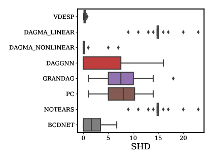
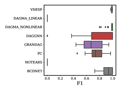
Figure 1: The structural Hamming distance (SHD, the lower the better) and the F1 score (the higher the better) on the synthetic linear data with $D=16$ and $\bar{E}=16$ on all graphs.

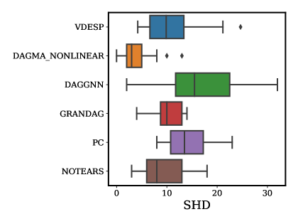
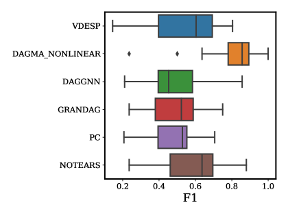
Figure 2: The structural Hamming distance (SHD, the lower the better) and the F1 score (the higher the better) on the synthetic nonlinear data with $D=16$ and $\bar{E}=16$ on all graphs.

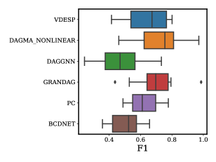
Figure 3: Results on real datasets: DREAM4 (Left), SACHS (middle) and SYNTREN (right). The F1 score (the higher the better) computed on the classification problem of predicting links including directionality. See Figure 6 in the appendix for SHD values.

We evaluate our approach on several synthetic, pseudo-real and real datasets used in the previous literature, comparing with competitive baseline algorithms under different metrics. In particular, we compare our method with BCDNET (Cundy et al., 2021), DAGMA_LINEAR and DAGMA_NOLINEAR (Bello et al., 2022) DAGGNN (Yu et al., 2019), GRANDAG (Lachapelle et al., 2019), NOTEARS (Zheng et al., 2018), DECI (Geffner et al., 2022) and JSP-GFN (Deleu et al., 2023). The results for DECI and JSP-GFN are not shown in the figures, as they were both found to underperform all the competing algorithms significantly, underlying the challenging nature of the problems we are addressing, especially in the nonlinear SEM case. This is discussed in the text in Section 8.3.

Metrics: As evaluation metrics we use the structural Hamming distance (SHD), which measures the number of changes (edge insertions/deletions/directionality change) needed in the predicted graph to match the underlying true graph. We also report the F1 score measured when formulating the problem as that of classifying links including directionality. We emphasize here that there is no perfect metric for our DAG estimation task and one usually should consider several metrics jointly. For example, we have found that some methods have the tendency to predict very sparse graphs and will obtain very low SHDs when the number of links in the underlying true graph is also very sparse.

8.1 Algorithm Settings

With the exception of BCDNET, DECI and JSP-GFN, where we use the implementation provided by the authors, we run the baseline algorithms using GCASTLE Zhang et al. (2021). Hyper-parameter setting was followed from the reference implementation and the recommendation by the authors (if any) in the original paper. However, for JSP-GFN we did try several configurations for their prior and model, none of which gave us significant performance improvements subject to our computational constraints (hours for each experiment instead of days).

For our algorithm (VDESP) we set the prior and posteriors to be Gaussians, used a link threshold for quantization of $0.5$. For experiments rather than the synthetic linear, we used a non-linear SEM as described in Section 6.1.2, i.e., based on a Gaussian exogenous noise model and the proposed architecture in Wehenkel & Louppe (2021) and learned its parameters via gradient-based optimization of the ELBO. Please see appendix for full details.

8.2 Synthetic Linear Datasets

Here we follow a similar setting to that of Geffner et al. (2022) and generate Erdős-Rényi (ER) graphs and scale-free (SF) graphs as described in Lachapelle et al. (2019, §A.5) where the SF graphs follow the preferential attachment model of Barabási (2009). We use $D=16$ nodes, $\bar{E}\in\{16,64\}$ expected edges and $N=1000$. We used a linear Gaussian SEM with the corresponding weights set to 1, biases to 0, mean zero and variance $0.01$. Experiments were replicated 10 times.

The results across all graphs (ER and SF) are shown in Figure 1. We see that our method VDESP performs the best among all competing approaches both in terms on the SHD and the F1 score. VDESP’s posterior exhibits a small variance, showing its confidence on its closeness to the underlying true graph. BCDNET performs very well too, given that it was specifically design for linear SEMs. Surprisingly, DAGMA_LINEAR performs poorly and even worse than DAGMA_NONLINEAR, perhaps indicating the hyper-parameters used in the former case were not adequate for this dataset. Additional results with a larger number of edges and separate for ER and SF graphs can be found in Appendix H.

8.3 Synthetic Nonlinear Datasets

Here we adopted a similar approach to that in Section 8.2 now with $D=16$, $\bar{E}=16$, $N=1000$, a nonlinear SEM given by a MLP with a noise model with mean zero and variance 1.

Results are shown in Figure 2, where we note that we have not included either BCDNET or DAGMA_LINEAR, as they were not designed to work on nonlinear SEMs. We see that VDESP is marginally better than DAGGNN, GRANDAG and performs similary to NOTEARS, while DAGMA_NONLINEAR achieves the best results on average. However, as mentioned throughout this paper, VDESP is much more informative as it provides a full posterior distribution over DAGs. We believe the fact that VDESP is competitive here is impressive as it is learning both a posterior over the DAG structure as well as the parameters of the nonlinear SEM (using the architecture proposed by Wehenkel & Louppe, 2021).

We also emphasize that we evaluated other Bayesian nonlinear approaches such as DECI and JSP-GFN but their results were surprisingly poor in terms of SHD and F1. This only highlights the challenges of learning a nonlinear SEM along with the DAG structure. However, it is possible that under a lot more tweaking of their hyper-parameters (for which we have very little guidance) and much larger computational constraints, one can get them to achieve comparable performance. More detailed results of this nonlinear setting are given in Appendix H.

8.4 Pseudo-Real & Real Datasets

SYNTREN: This pseudo-real dataset was used by Lachapelle et al. (2019) and generated using the SynTReN generator of Van den Bulcke et al. (2006). The data represent genes and their level of expression in transcriptional regulatory networks. The generated gene expression data approximates experimental data. It has $10$ sets of $N=500$ observations, $D=20$ variables and $\bar{E}=33.3$ edges.

DREAM4: This real dataset is from the Dream4 in-silico network challenge on gene regulation as used previously by Annadani et al. (2021). We use the multi-factorial dataset with $D=10$ nodes and $N=10$ observations of which we have $5$ different sets of observations and ground truth graphs, with $\bar{E}=14.2$ edges.

SACHS: This real dataset is concerned with the discovery of protein signaling networks from flow cytometry data as described in Sachs et al. (2005) with $D=11$ variables, $N=4,200$ observations with $10$ different sets of observations and ground truth graphs, with $\bar{E}=17.0$ edges.

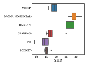
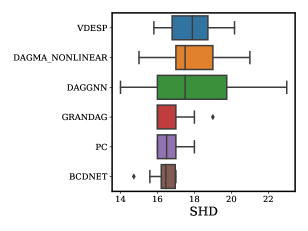
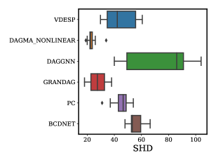
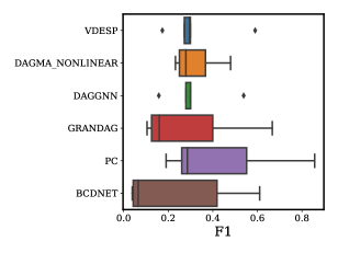
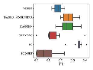
Figure 6: Results on real datasets: DREAM4 (Left), SACHS (middle) and SYNTREN (right). The top row shows the structural Hamming distance (SHD, the lower the better), while the bottom row shows the F1 score (the higher the better). The latter computed on the classification problem of predicting links including directionality.

Results are shown in Figure 3. On these datasets we have assumed that one has very little knowledge of the underlying SEM and, therefore, as with the synthetic nonlinear data, we have excluded DAGMA_LINEAR form this analysis. However, we show the results for BCDNET as a comparison to another Bayesian framework. We see that VDESP outperforms BCDNET consistently in terms of F1 across datasets, while providing competitive SHD values throughout, even clearly outperforming DAGMA_NONLINEAR and DAGGNN on DREAM4 (top left of Figure 6 in the appendix) and DAGGNN on SYNTREN (top right of Figure 6 in the appendix).

Understanding Alzheimer’s disease: Alzheimer’s disease (AD) is a degenerative brain disease and the most common form of dementia. It is estimated that around 55 million people are living with AD worldwide. The public health, social and economic impact of AD is, therefore, an important problem. We used VDESP to understand the progression and diagnosis of the disease. Overall, VDESP’s predictions uncovered what is known to be the “gold standard” for relationships between AD biomarkers and cognition while, using samples from the posterior, hinting at interesting alternative explanations of the disease. See Appendix I for details.

9 Conclusion

We have presented a Bayesian DAG structure estimation method that inherently encodes the acyclicity constraint by construction on its model (and posterior) distributions. It does so by considering joint distributions on an augmented space of permutations and graphs. Given a node ordering sampled from a permutation distribution, our model defines simple and consistent distributions over DAGs. We have developed a variational inference method for estimating the posterior distribution over DAGs and have shown that it can outperform competitive benchmarks across a variety of synthetic, pseudo-real and real problems. As currently implemented, VDESP does come with its own limitations. In particular, we believe that incorporating better prior knowledge through strongly sparse and/or hierarchical distributions may make our method much more effective. We will explore this direction in future work.

Impact Statement

This paper presents work whose goal is to advance the field of Machine Learning. There are many potential societal consequences of our work, none which we feel must be specifically highlighted here.

Appendix A Distribution of the Minimum in the Gamma/Exponential Model

We are interested in computing $Pr(I=k)$ so we have

$$\text{Pr}(I=k) =\int_{0}^{\infty}p(V_{k}=v)\text{Pr}(\forall_{i\neq k}V_{i}>v)dv,$$ (15)

$$=\int_{0}^{\infty}p(V_{k}=v)\prod_{i\neq k}(1-F_{i}(v))dv,$$ (16)

where $p(V_{k}=v)$ is the exponential distribution defined in Equation 3 and $F_{i}(v)$ is the cumulative distribution function of $V_{i}$. When each of the variables follows an exponential distribution as given by Equation 3, we have that:

$$\text{Pr}(I=k) =\frac{1}{\gamma_{k}}\int_{0}^{\infty}\exp(-\frac{v}{\gamma_{k}})\prod_{i\neq k}\exp(-\frac{v}{\gamma_{i}})dx$$ (17)

$$=\frac{1}{\gamma_{k}}\int_{0}^{\infty}\exp\left(-\sum_{i=1}^{N}\frac{1}{\gamma_{i}}v\right)dv$$ (18)

$$=\frac{\beta_{k}}{\beta_{1}+\ldots+\beta_{N}},$$ (19)

Appendix B Alternative Sampling of Permutations from the Gamma Model

As explained in the main paper, we can also sample from this model by using categorical distributions based on Equation 6. In this case we simply sample from categorical distributions one at a time on a reduced set (which will give us the argmin on the reduced set):

1. Set $\mathcal{B}=\{\beta_{1},\ldots,\beta_{D}\}$ with $\beta_{j}\in\mathcal{B}$

2. For $i=0,\ldots,D-1$

   1. Sample element $\pi_{i}$ from a categorical distribution with parameters $\{\theta_{k}\}_{k=1}^{|\mathcal{B}|}$, $\theta_{k}=\frac{\beta_{k}}{\sum_{j}\beta_{j}}$ with $\beta_{j}\in\mathcal{B}$

   2. Set $\mathcal{B}=\mathcal{B}-\{\pi_{i}\}$

Appendix C Gumbel-Max Constructions of Distributions over Permutations

Here we describe the Gumbel-Max construction of distributions over permutations, as given, e.g., in Grover et al. (2019). this construction is parameterized by a vector of log scores ${\boldsymbol{\mathbf{s}}}$, which are corrupted with noise drawn from a Gumbel distribution. The resulting corrupted scores are then sorted in descending order as follows:

1. Let ${\boldsymbol{\mathbf{s}}}$ be a vector of scores

2. Sample $g_{i}$ from a Gumbel distribution with location $\mu=0$ and scale $\sigma>0$

   1. $z_{i}\sim\text{Uniform}(0,1)$

   2. $g_{i}=\mu-\sigma\log(-\log(z_{i}))$

3. Let $\tilde{{\boldsymbol{\mathbf{s}}}}$ be the vector of perturbed scores with Gumbel noise such that:
   $\tilde{s_{i}}=\sigma\log s_{i}+g_{i}$

4. ${\boldsymbol{\mathbf{\pi}}}=\texttt{argsort}(\tilde{{\boldsymbol{\mathbf{s}}}},\texttt{descending=True})$,

where we emphasize the corrupted scores are sorted in descending order. As we will see below, the distribution over permutations generated with the above procedure is given by the RHS of Equation 6 with ${\boldsymbol{\mathbf{\beta}}}={\boldsymbol{\mathbf{s}}}$. In our experiments, we use $\sigma=1$.

C.1 Relation to Gamma Construction

Here we compare our Gumbel-Max construction with the Gamma/exponential construction described in Section 5.1.3 (based on the model proposed in Stern (1990)). This is interesting because Yellott (1977) has shown that the Plackett-Luce model can only be obtained via the Gumble-Max mechanism, implying that both approaches should be equivalent.

It is shown in Yellott (1977) that the distribution over permutations generated by the above procedure with identical Gumbel scales $\sigma$ is given by Equation 6 with ${\boldsymbol{\mathbf{\beta}}}={{\boldsymbol{\mathbf{s}}}}$. This means that, essentially, our Exponential-based sampling process in Section 5.1.3 is equivalent to the one above. To show this, let us retake our Exponential samples (before the argsort operation):

$$x_{i} =-\beta_{i}^{-1}\log(1-z_{i})$$ (20)

$$=-\beta_{i}^{-1}\log(z_{i}),$$ (21)

as $1-z_{i}\sim\text{Uniform}(0,1)$. Now we (i) make $s_{i}:=\beta_{i}$; (ii) take a $\log$ transform of the above variable, which is a monotonic transformation and preserves ordering; and (iii) multiply by $-\sigma$ so that we reverse the permutation to descending order:

$$-\sigma\log(x_{i}) =-\sigma\log(\beta_{i}^{-1}(-\log z_{i})),$$ (22)

$$=\sigma\log s_{i}-\sigma\log(-\log z_{i}),$$ (23)

$$=\tilde{s}_{i},$$ (24)

giving us exactly the noisy scores of the Gumbel-Max construction above. Presumably, this parameterization is more numerically stable as we are taking the log twice.

More generally, we can show that we can transform a Gumbel-distributed variable $g\sim\text{Gumbel}(\mu,\sigma)$ into an exponential distribution. Let $z\sim\text{Uniform}(0,1)$ then, as described above:

$$g=\mu-\sigma\log(-\log z)$$ (25)

follows a Gumbel distribution with location $\mu$ and scale $\sigma>0$. Now, consider the following monotonic transformation:

$$x =\exp\left(-\frac{g+\sigma\log\beta-\mu}{\sigma}\right)$$ (26)

$$=-\beta^{-1}\log(z).$$ (27)

Thus, $x\sim\text{Exponential}(\beta)$.

Appendix D Conventions & Implementation

Here we define some conventions and assumptions in our implementation.

D.1 Directed Graph Representation via Adjacency Matrices

As mentioned in the main text, we represent a directed graph with an adjacency matrix ${\boldsymbol{\mathbf{A}}}$, where $A_{ij}=1$ iff there is an arrow from node $i$ to node $j$, i.e., $i\rightarrow j$ and $A_{ij}=0$ otherwise. In the case of DAGs, this means that the matrix has zeros in its diagonal and $A_{ij}=1$ implies $A_{ji}=0$. Moreover, given a permutation in topological order (or reverse topological order) the adjacency matrix would have an upper triangular (or lower triangular) structure if one were to order the rows and columns according to that permutation.

D.2 Topological Order

A standard topological order given by a permutation vector ${\boldsymbol{\mathbf{\pi}}}=[\pi_{1},\ldots,\pi_{D}]$ defines constraints in a DAG such that arrows can only be drawn from left to right. For example, for the ordering ${\boldsymbol{\mathbf{\pi}}}=[2,0,1]$ the DAG $2\rightarrow 0\rightarrow 1$ is valid under such ordering but any DAG where, for example, arrows are drawn from $1$ is invalid. Similarly, any DAG containing the link $0\rightarrow 2$ is also invalid.

This places constraints on the set of admissible adjacency matrices under the given permutation. In particular, we are interested in representing this set via a distribution parameterized by a parameter matrix ${\boldsymbol{\mathbf{\Theta}}}$, where $\Theta_{ij}>0$ indicates that there is a non-zero probability of drawing a link $i\rightarrow j$. In this case, it is easy to see that the probability matrix ${\boldsymbol{\mathbf{\Theta}}}$ consistent with the permutation ${\boldsymbol{\mathbf{\pi}}}$ satisfies $\Theta_{\pi_{i}\pi_{j}}=0$ $\forall i>j$.

D.3 Reverse Topological Order

Analogously, in a reverse topological order given by permutation vector ${\boldsymbol{\mathbf{\pi}}}$, arrows can only be drawn from right to left. Thus, we see that the probability matrix consistent with the permutation ${\boldsymbol{\mathbf{\pi}}}$ satisfies $\Theta^{\text{r}}_{\pi_{i}\pi_{j}}=0$ $\forall i<j$.

D.4 Permutation Matrices

In order to express all our operations using linear algebra, which in turn allows us to apply relaxations and back-propagate gradients, we represent a permutation ${\boldsymbol{\mathbf{\pi}}}=[\pi_{1},\ldots,\pi_{D}]$ via a $D$-dimensional permutation matrix ${\boldsymbol{\mathbf{\Pi}}}$ such as that $\Pi_{ij}=1$ iff $j=\pi(i)$ and $\Pi_{ij}=0$ otherwise. This means that we can recover the permutation ${\boldsymbol{\mathbf{\pi}}}$ by computing the max over the columns of ${\boldsymbol{\mathbf{\Pi}}}$, i.e., in Pythonic notation $\mathtt{{\boldsymbol{\mathbf{\pi}}}=\max({\boldsymbol{\mathbf{\Pi}}},dim=1)}$.

D.5 Distributions over DAGs

Let ${\boldsymbol{\mathbf{L}}}$ be a $D$-dimensional strictly lower diagonal matrix, i.e., $L_{ij}=0$, $\forall i<j$ and $L_{ij}=1$ otherwise. Similarly, let ${\boldsymbol{\mathbf{U}}}$ be a $D$-dimensional strictly upper diagonal matrix. Given a permutation matrix ${\boldsymbol{\mathbf{\Pi}}}$ the corresponding DAG distributions are:

$${\boldsymbol{\mathbf{\Theta}}} ={\boldsymbol{\mathbf{\Pi}}}^{\top}{\boldsymbol{\mathbf{U}}}{\boldsymbol{\mathbf{\Pi}}},$$ (28)

$${\boldsymbol{\mathbf{\Theta}}}^{\text{r}} ={\boldsymbol{\mathbf{\Pi}}}^{\top}{\boldsymbol{\mathbf{L}}}{\boldsymbol{\mathbf{\Pi}}}.$$ (29)

We will show this for the standard case of topological order. Consider Equation 28:

$$\Theta_{ij} =\sum_{m}\sum_{k}({\boldsymbol{\mathbf{\Pi}}}^{\top})_{ik}U_{km}{\boldsymbol{\mathbf{\Pi}}}_{mj}$$ (30)

$$=\sum_{m}\sum_{k}{\boldsymbol{\mathbf{\Pi}}}_{ki}U_{km}{\boldsymbol{\mathbf{\Pi}}}_{mj}.$$ (31)

this, for a given permutation ${\boldsymbol{\mathbf{\pi}}}$, we can express:

$$\Theta_{\pi_{k}\pi_{m}}={\boldsymbol{\mathbf{\Pi}}}_{k\pi_{k}}U_{km}{\boldsymbol{\mathbf{\Pi}}}_{m\pi_{m}},$$ (32)

which, as ${\boldsymbol{\mathbf{U}}}$ is an upper triangular matrix, implies $\Theta_{\pi_{k}\pi_{m}}=0$, $\forall k>m$.

For clarity and consistency with previous literature, we emphasize our convention $\Theta_{ij}$ indicates the probability of a link $i\rightarrow j$. If we were to use the transpose definition of the space of adjacency matrices ${\boldsymbol{\mathbf{\Phi}}}={\boldsymbol{\mathbf{\Theta}}}^{\top}$ indicating the probability of a link $\Phi_{ij}:j\rightarrow i$, as for example in Dallakyan & Pourahmadi (2021), then we would have (in the case of a topological ordering) ${\boldsymbol{\mathbf{\Phi}}}={\boldsymbol{\mathbf{\Pi}}}^{\top}{\boldsymbol{\mathbf{L}}}{\boldsymbol{\mathbf{\Pi}}}$.

Appendix E The Relaxed Bernoulli Distribution

Here we follow the description in Maddison et al. (2017). A random variable $A\in(0,1)$ follows a relaxed Bernoulli distribution, also known as a binary Concrete distribution, denoted as $A\sim\text{RelaxedBernoulli}(\tau,\alpha)$ with location parameter $\alpha\in(0,\infty)$ and temperature $\tau\in(0,\infty)$ if its density is given by:

$$\text{RelaxedBernoulli}(a;\tau,\alpha):=p(a\,|\,\tau,\alpha)=\frac{\tau\alpha a^{-\tau-1}(1-a)^{-\tau-1}}{(\alpha a^{-\tau}+(1-a)^{-\tau})^{2}}.$$ (33)

For our purposes, we are interested in sampling from this distribution and computing the log probability of variables under this model. Below we describe how to do these operations based on a parameterization using Logistic distributions.

E.1 Sampling

Let us define the logistic sigmoid function and its inverse (the logit function) as

$$\sigma(x) :=\frac{1}{1+\exp(-x)},$$ (34)

$$\sigma^{-1}(x) :=\log\frac{x}{1-x}.$$ (35)

In order to sample $a\sim\text{RelaxedBernoulli}(\tau,\alpha)$ we do the following:

1. Sample $L\sim\text{Logistic}(0,1)$

   1. $U\sim\text{Uniform}(0,1)$

   2. $L=\log(U)-\log(1-U)$

2. $\displaystyle b=\frac{\log\alpha+L}{\tau}$

3. $a=\sigma(b)$.

E.2 Log Density Computation

Given a realization $b$ (before applying $\sigma(b)$), we also require the computation of its log density under the relaxed Bernoulli model. With the parameterization above using the Logistic distribution, it is easy to get this density by using the change-of-variable (transformation) formula to obtain:

$$\log p(b;\tau,\alpha)=\log\tau+\log\alpha-\tau b-2\log\left(1+\exp(\log\alpha-\tau b)\right).$$ (36)

In order to obtain the log density of $0<a<1$ under the relaxed Bernoulli model, we need to apply the change of variable formula again, as $a=\sigma(b))$,

$$\log p(a;\tau,\alpha)=\log\tau+\log\alpha-\tau\sigma^{-1}(a)-2\log\left(1+\exp(\log\alpha-\tau\sigma^{-1}(a))\right)-\log a-\log(1-a).$$ (37)

E.3 Probability Re-parameterization

The relaxed Bernoulli distribution has several interesting properties described in Maddison et al. (2017). In particular, the rounding property (Maddison et al., 2017, ,Proposition 2), establishes that if $X\sim\text{RelaxedBernoulli}(\tau,\alpha)$:

$$\mathbb{P}(X>0.5)=\frac{\alpha}{1+\alpha}.$$ (38)

Therefore, our implementation adopts Pytorch parameterization using a “probability” parameter $\theta\in(0,1)$ so that

$$\theta:=\frac{\alpha}{1+\alpha}.$$ (39)

Appendix F Relaxed Distributions over Permutations

We have seen that sampling from our distributions over permutations requires the argsort operator which is not differentiable. Therefore, in order to back-propagate gradients and estimate the parameters of our posterior over permutations, we relax this operator following the approach of Prillo & Eisenschlos (2020),

$$\text{SoftSort}(\tilde{{\boldsymbol{\mathbf{s}}}}):=\text{softmax}\left(\frac{\mathcal{L}_{d}\left(\texttt{sort}(\tilde{{\boldsymbol{\mathbf{s}}}}){\boldsymbol{\mathbf{1}}}^{\scriptscriptstyle T},{\boldsymbol{\mathbf{1}}}\tilde{{\boldsymbol{\mathbf{s}}}}^{\scriptscriptstyle T}\right)}{\tau_{\pi}}\right),$$ (40)

where $\mathcal{L}_{d}(\cdot,\cdot)$ is a semi-metric function applied point-wise that is differentiable almost everywhere; $\tau_{\pi}$ is a temperature parameter; and $\text{softmax}(\cdot)$ is the row-wise softmax function. Here we have assumed that $\texttt{sort}(\tilde{{\boldsymbol{\mathbf{s}}}}):=\texttt{sort}(\tilde{{\boldsymbol{\mathbf{s}}}},\texttt{descending=True})$, which applies directly to the Gumbel-Max construction. In the case of the Gamma construction, which assumes ascending orders, we simply pass in the negative of the corresponding scores. We note that Equation 40 uses $\texttt{sort}(\cdot)$, which unlike the $\texttt{argsort}(\cdot)$, is a differentiable operation.

F.1 Sampling

Sampling from our relaxed distributions over permutations is done by simply replacing the $\texttt{argsort}(\cdot)$ operation used in the vanilla (hard) permutation distribution with the $\text{SoftSort}(\cdot)$ function above. This function returns, in fact, a permutation matrix ${\boldsymbol{\mathbf{\Pi}}}$ which is used as a conditioning value in the DAG distribution, as explained in Section D.5, and as input to the log probability computation in the KL term over permutations.

F.2 Log Probability Computation

The log probability of a permutation matrix ${\boldsymbol{\mathbf{\Pi}}}$ given a distribution with parameters ${\boldsymbol{\mathbf{\beta}}}$ (in the case of the Gamma construction) can be computed using Equation 6, where ${\boldsymbol{\mathbf{\beta}}}_{\boldsymbol{\mathbf{\pi}}}$ are the permuted parameters given by:

$${\boldsymbol{\mathbf{\beta}}}_{\boldsymbol{\mathbf{\pi}}}={\boldsymbol{\mathbf{\Pi}}}{\boldsymbol{\mathbf{\beta}}}.$$ (41)

In the case of the Gumbel-Max construction, ${\boldsymbol{\mathbf{\beta}}}_{\boldsymbol{\mathbf{\pi}}}$ is obtained by reversing the order of ${\boldsymbol{\mathbf{s}}}_{\boldsymbol{\mathbf{\pi}}}={\boldsymbol{\mathbf{\Pi}}}{\boldsymbol{\mathbf{s}}}$.

Appendix G Full Objective Function Using Monte Carlo Expectations

We retake our objective function:

$$\begin{split}\mathcal{L}=\mathbb{E}_{q_{\pi}({\boldsymbol{\mathbf{\pi}}}\,|\,r,{\boldsymbol{\mathbf{\beta}}})}\left[\log q_{\pi}({\boldsymbol{\mathbf{\pi}}}\,|\,r,{\boldsymbol{\mathbf{\beta}}})-\log p({\boldsymbol{\mathbf{\pi}}}\,|\,r_{0},{\boldsymbol{\mathbf{\beta}}}_{0})\right]+\mathbb{E}_{q_{\pi}({\boldsymbol{\mathbf{\pi}}}\,|\,r,{\boldsymbol{\mathbf{\beta}}})q_{\mathcal{G}}(\mathcal{G}\,|\,{\boldsymbol{\mathbf{\pi}}},{\boldsymbol{\mathbf{\Theta}}})}\left(\log q_{\mathcal{G}}(\mathcal{G}\,|\,{\boldsymbol{\mathbf{\pi}}},{\boldsymbol{\mathbf{\Theta}}})-\log p(\mathcal{G}\,|\,{\boldsymbol{\mathbf{\pi}}},{\boldsymbol{\mathbf{\Theta}}}_{0})\right)\\ +\mathbb{E}_{q_{\pi}({\boldsymbol{\mathbf{\pi}}}\,|\,r,{\boldsymbol{\mathbf{\beta}}})q_{\mathcal{G}}(\mathcal{G}\,|\,{\boldsymbol{\mathbf{\pi}}},{\boldsymbol{\mathbf{\Theta}}})}\sum_{n=1}^{N}\log p({\boldsymbol{\mathbf{x}}}^{(n)}\,|\,\mathcal{G},{\boldsymbol{\mathbf{\phi}}})\end{split}$$ (42)

Appendix H Additional Results

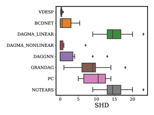
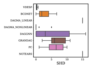
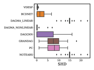
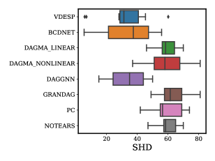
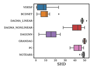
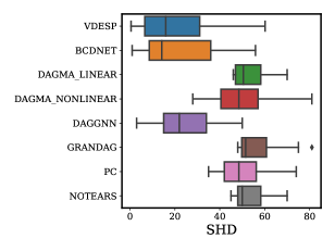
Figure 4: Results on the synthetic linear data with $D=16$ variables (nodes) on ER (left), SF (middle), and all (right) graphs. The top row is with $\bar{E}=16$ edges and the bottom row with $\bar{E}=64$ edges, respectively.

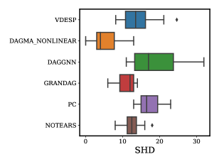
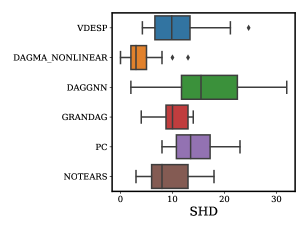
Figure 5: Results on the synthetic nonlinear data with $D=16$ and $E=16$ on ER (left), SF (middle), and all (right) graphs.

Appendix I Additional Results on Alzheimer’s Data

We applied VDESP for discovering the causal relationships between Alzheimer disease biomarkers and cognition. The source data were made publicly available by the Alzheimer’s Disease Neuroimaing Initiative (ADNI). These data have been used previously to evaluate causal discovery algorithms (Shen et al., 2020) because a “gold standard” graph for these data is known.

For our experiments we focused on $7$ variables which include demographic information age (AGE) and years of education (PTEDUCAT) along with biological variables which include fludeoxyglucose PET (FDG), amyloid beta (ABETA) phosphorylated tau (PTAU), and the aplipoprotoen E (APOE4) $\epsilon$ 4 allele. The last variable of interest represents the participant’s clinically assessed level of cognition (DX) indicating one of three levels: normal, mild cognitive impairment (MCI) and early Alzheimer’s Disease (AD). Ultimately, we want to infer the causal influences on DX.

The data is collected from participants as part of the first two phases of ADNI that commenced in 2003. In total, we have data for $1336$ individuals after removing those with missing values.

The results are shown in Figures 7 and 8. We see that VDESP uncovered the main underlying graph structure, while hinting at different explanations of the data which may require further investigation.

Figure 7: The true graph on the Alzheimer dataset (left) and the mean posterior graph predicted by VDESP.

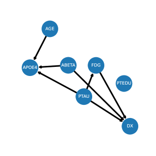
Figure 8: VDESP’s Posterior samples on the Alzheimer dataset.

Appendix J VDESP Hyper-Parameters and Reproducibility

In all our experiments we train our model by optimizing the ELBO using the Adam optimizer with learning rate 0.001. We set the temperature parameter of our relaxed permutation distributions to 0.5. The scores of the permutation distributions were set to give rise to uniform distributions and the posterior was initialized the the same values. We use Gaussians for the DAG distributions with zero mean prior and prior and initial posterior scales set to $0.1$.

For the linear dataset we used $100$ permutation samples and $100$ DAG samples per permutation and optimize for $75000$ iterations. For the synthetic non-linear data we set the number number of permutation samples = $2$, number of DAG samples = $2$ and training epochs = $30000$ while we initialized the non-linear SEM noise scale = $1.0$.

For the real data using the non-linear SEM we used a fixed noise scale = {$0.01$, $0.25$, $0.3$}, number of permutation samples = {$10$, $10$, $5$}, number of DAG samples = {$15$, $15$, $5$} and training epochs = {$5000$, $5000$, $15000$} for DREAM4, SACHS, and SYNTREN respectively.

In all cases when using a non-linear SEM, our model had a single hidden layer with $10$ neurons and sigmoid activation.

For reproducibility purposes, we will make our code publicly available upon acceptance.

References

- Annadani et al. (2021) Annadani, Y., Rothfuss, J., Lacoste, A., Scherrer, N., Goyal, A., Bengio, Y., and Bauer, S. Variational causal networks: Approximate Bayesian inference over causal structures. arXiv preprint arXiv:2106.07635, 2021.
- Barabási (2009) Barabási, A. L. Scale-free networks: A decade and beyond. Science, 325(5939):412–413, 2009. ISSN 00368075. doi: 10.1126/science.1173299.
- Bello et al. (2022) Bello, K., Aragam, B., and Ravikumar, P. DAGMA: Learning DAGs via M-matrices and a Log-Determinant Acyclicity Characterization. Number Neural Information Processing Systems, 2022. URL http://arxiv.org/abs/2209.08037.
- Bengio et al. (2013) Bengio, Y., Léonard, N., and Courville, A. Estimating or Propagating Gradients Through Stochastic Neurons for Conditional Computation. arXiv preprint arXiv:1308.3432, pp. 1–12, 2013. URL http://arxiv.org/abs/1308.3432.
- Bengio et al. (2023) Bengio, Y., Lahlou, S., Deleu, T., Hu, E. J., Tiwari, M., and Bengio, E. Gflownet foundations. Journal of Machine Learning Research, 24(210):1–55, 2023.
- Bühlmann et al. (2014) Bühlmann, P., Peters, J., and Ernest, J. CAM: Causal additive models, high-dimensional order search and penalized regression. Annals of Statistics, 42(6):2526–2556, 2014. ISSN 00905364. doi: 10.1214/14-AOS1260.
- Chickering (2002) Chickering, D. M. Optimal structure identification with greedy search. Journal of machine learning research, 3(Nov):507–554, 2002.
- Chickering et al. (2004) Chickering, M., Heckerman, D., and Meek, C. Large-sample learning of bayesian networks is np-hard. Journal of Machine Learning Research, 5:1287–1330, 2004.
- Cundy et al. (2021) Cundy, C., Grover, A., and Ermon, S. BCD Nets: Scalable Variational Approaches for Bayesian Causal Discovery. Advances in Neural Information Processing Systems, 9(NeurIPS):7095–7110, 2021. ISSN 10495258.
- Dallakyan & Pourahmadi (2021) Dallakyan, A. and Pourahmadi, M. Learning Bayesian Networks through Birkhoff Polytope: A Relaxation Method. pp. 1–10, 2021. URL http://arxiv.org/abs/2107.01658.
- Deleu et al. (2023) Deleu, T., Nishikawa-Toomey, M., Subramanian, J., Malkin, N., Charlin, L., and Bengio, Y. Joint Bayesian Inference of Graphical Structure and Parameters with a Single Generative Flow Network. In NeurIPS, 2023.
- Geffner et al. (2022) Geffner, T., Antoran, J., Foster, A., Gong, W., Ma, C., Kiciman, E., Sharma, A., Lamb, A., Kukla, M., Pawlowski, N., et al. Deep end-to-end causal inference. arXiv preprint arXiv:2202.02195, 2022.
- Glymour et al. (2019) Glymour, C., Zhang, K., and Spirtes, P. Review of causal discovery methods based on graphical models. Frontiers in Genetics, 10(JUN):1–15, 2019. ISSN 16648021. doi: 10.3389/fgene.2019.00524.
- Grover et al. (2019) Grover, A., Wang, E., Zweig, A., and Ermon, S. Stochastic optimization of sorting networks via continuous relaxations. In 7th International Conference on Learning Representations, ICLR 2019, pp. 1–23, 2019.
- Han et al. (2016) Han, S. W., Chen, G., Cheon, M.-S., and Zhong, H. Estimation of directed acyclic graphs through two-stage adaptive lasso for gene network inference. Journal of the American Statistical Association, 111(515):1004–1019, 2016.
- Hoyer et al. (2008) Hoyer, P., Janzing, D., Mooij, J. M., Peters, J., and Schölkopf, B. Nonlinear causal discovery with additive noise models. Advances in neural information processing systems, 21, 2008.
- Imbens (2020) Imbens, G. W. Potential outcome and directed acyclic graph approaches to causality: Relevance for empirical practice in economics. Journal of Economic Literature, 58:1129–1179, 2020.
- Lachapelle et al. (2019) Lachapelle, S., Brouillard, P., Deleu, T., and Lacoste-Julien, S. Gradient-Based Neural DAG Learning. (2018):1–23, 2019. URL http://arxiv.org/abs/1906.02226.
- Lauritzen & Spiegelhalter (1988) Lauritzen, S. L. and Spiegelhalter, D. J. Local computations with probabilities on graphical structures and their application to expert systems. Journal of the Royal Statistical Society: Series B (Methodological), 50:157–224, 1988.
- Lippe et al. (2021) Lippe, P., Cohen, T., and Gavves, E. Efficient neural causal discovery without acyclicity constraints. arXiv preprint arXiv:2107.10483, 2021.
- Lorch et al. (2021) Lorch, L., Rothfuss, J., Schölkopf, B., and Krause, A. DiBS: Differentiable Bayesian Structure Learning. Advances in Neural Information Processing Systems, 29(NeurIPS):24111–24123, 2021. ISSN 10495258.
- Maddison et al. (2017) Maddison, C. J., Mnih, A., and Teh, Y. W. The concrete distribution: A continuous relaxation of discrete random variables. 5th International Conference on Learning Representations, ICLR 2017 - Conference Track Proceedings, pp. 1–20, 2017.
- Madigan et al. (1994) Madigan, D., Gavrin, J., and Raftery, A. E. Enhancing the predictive performance of bayesian graphical models. 1994.
- Mooij et al. (2011) Mooij, J. M., Janzing, D., Heskes, T., and Schölkopf, B. On causal discovery with cyclic additive noise models. In Shawe-Taylor, J., Zemel, R., Bartlett, P., Pereira, F., and Weinberger, K. (eds.), Advances in Neural Information Processing Systems, volume 24. Curran Associates, Inc., 2011. URL https://proceedings.neurips.cc/paper/2011/file/d61e4bbd6393c9111e6526ea173a7c8b-Paper.pdf.
- Murphy (2023) Murphy, K. P. Probabilistic Machine Learning. MIT Press, Cambridge, MA, USA, 2023.
- Ni et al. (2019) Ni, Y., Stingo, F. C., and Baladandayuthapani, V. Bayesian graphical regression. Journal of the American Statistical Association, 114:184–197, 2019.
- Pearl (1988) Pearl, J. Probabilistic Reasoning in Intelligent Systems. Morgan Kaufmann, San Francisco, CA, USA, 1988.
- Prillo & Eisenschlos (2020) Prillo, S. and Eisenschlos, J. SoftSort: A continuous relaxation for the argsort operator. In III, H. D. and Singh, A. (eds.), Proceedings of the 37th International Conference on Machine Learning, volume 119 of Proceedings of Machine Learning Research, pp. 7793–7802. PMLR, 13–18 Jul 2020.
- Sachs et al. (2005) Sachs, K., Perez, O., Pe’er, D., Lauffenburger, D. A., and Nolan, G. P. Causal protein-signaling networks derived from multiparameter single-cell data. Science, 308(5721):523–529, 2005.
- Shen et al. (2020) Shen, X., Ma, S., Vemuri, P., Simon, G., and the Alzheimer’s Disease Neuroimaging Initiatie. Challenges and opportunities with causal discovery algorithms: Application to alzheimer’s pathophysiology. Scientific Reports, 10, 2020. doi: 10.1038/s41598-020-59669-x.
- Shimizu et al. (2006) Shimizu, S., Hoyer, P. O., Hyvärinen, A., Kerminen, A., and Jordan, M. A linear non-gaussian acyclic model for causal discovery. Journal of Machine Learning Research, 7(10), 2006.
- Shimizu et al. (2011) Shimizu, S., Inazumi, T., Sogawa, Y., Hyvärinen, A., Kawahara, Y., Washio, T., Hoyer, P. O., and Bollen, K. DirectLiNGAM: A direct method for learning a linear non-gaussian structural equation model. Journal of Machine Learning Research, 12:1225–1248, 2011. ISSN 15324435.
- Spirtes et al. (2000) Spirtes, P., Glymour, C. N., and Scheines, R. Causation, prediction, and search. MIT press, 2000.
- Stern (1990) Stern, H. Models for distributions on permutations. Journal of the American Statistical Association, 85(410):558–564, 1990. ISSN 1537274X. doi: 10.1080/01621459.1990.10476235.
- Su et al. (2013) Su, C., Andrew, A., Karagas, M. R., and Borsuk, M. E. Using bayesian networks to discover relations between genes, environment, and disease. BioData mining, 6(1):1–21, 2013.
- Tennant et al. (2021) Tennant, P. W. G., Murray, E. J., Arnold, K. F., Berrie, L., Fox, M. P., Gadd, S. C., Harrison, W. J., Keeble, C., Ranker, L. R., Textor, J., Tomova, G. D., Gilthorpe, M. S., and Ellison, G. T. H. Use of directed acyclic graphs (dags) to identify confounders in applied health research: Review and recommendations. International Journal of Epidemiology, 50:620–632, 2021.
- Van den Bulcke et al. (2006) Van den Bulcke, T., Van Leemput, K., Naudts, B., van Remortel, P., Ma, H., Verschoren, A., De Moor, B., and Marchal, K. Syntren: a generator of synthetic gene expression data for design and analysis of structure learning algorithms. BMC bioinformatics, 7:1–12, 2006.
- Vowels et al. (2022) Vowels, M. J., Camgoz, N. C., and Bowden, R. D’ya like dags? a survey on structure learning and causal discovery. ACM Computing Surveys, 55:1–36, 2022.
- Wang et al. (2022) Wang, B., Wicker, M. R., and Kwiatkowska, M. Tractable uncertainty for structure learning. In Chaudhuri, K., Jegelka, S., Song, L., Szepesvari, C., Niu, G., and Sabato, S. (eds.), Proceedings of the 39th International Conference on Machine Learning, volume 162 of Proceedings of Machine Learning Research, pp. 23131–23150. PMLR, 17–23 Jul 2022. URL https://proceedings.mlr.press/v162/wang22ad.html.
- Wehenkel & Louppe (2021) Wehenkel, A. and Louppe, G. Graphical normalizing flows. In Banerjee, A. and Fukumizu, K. (eds.), Proceedings of The 24th International Conference on Artificial Intelligence and Statistics, volume 130 of Proceedings of Machine Learning Research, pp. 37–45. PMLR, 13–15 Apr 2021. URL https://proceedings.mlr.press/v130/wehenkel21a.html.
- Yellott (1977) Yellott, J. I. The relationship between Luce’s Choice Axiom, Thurstone’s Theory of Comparative Judgment, and the double exponential distribution. Journal of Mathematical Psychology, 15(2):109–144, 1977. ISSN 10960880. doi: 10.1016/0022-2496(77)90026-8.
- Yu et al. (2019) Yu, Y., Chen, J., Gao, T., and Yu, M. DAG-GNN: DAG structure learning with graph neural networks. 36th International Conference on Machine Learning, ICML 2019, 2019-June:12395–12406, 2019.
- Zhang & Hyvärinen (2009) Zhang, K. and Hyvärinen, A. On the identifiability of the post-nonlinear causal model. In 25th Conference on Uncertainty in Artificial Intelligence (UAI 2009), pp. 647–655. AUAI Press, 2009.
- Zhang et al. (2021) Zhang, K., Zhu, S., Kalander, M., Ng, I., Ye, J., Chen, Z., and Pan, L. gcastle: A python toolbox for causal discovery, 2021.
- Zheng et al. (2018) Zheng, X., Aragam, B., Ravikumar, P., and Xing, E. P. Dags with no tears: Continuous optimization for structure learning. Advances in Neural Information Processing Systems, 2018-Decem(1):9472–9483, 2018. ISSN 10495258.