Can Large Language Models Learn Independent Causal Mechanisms?

Abstract

Despite impressive performance on language modelling and complex reasoning tasks, Large Language Models (LLMs) fall short on the same tasks in uncommon settings or with distribution shifts, exhibiting some lack of generalisation ability. This issue has usually been alleviated by feeding more training data into the LLM. However, this method is brittle, as the scope of tasks may not be readily predictable or may evolve, and updating the model with new data generally requires extensive additional training. By contrast, systems, such as causal models, that learn abstract variables and causal relationships can demonstrate increased robustness against changes in the distribution. One reason for this success is the existence and use of Independent Causal Mechanisms (ICMs) representing high-level concepts that only sparsely interact. In this work, we apply two concepts from causality to learn ICMs within LLMs. We develop a new LLM architecture composed of multiple sparsely interacting language modelling modules. We introduce a routing scheme to induce specialisation of the network into domain-specific modules. We also present a Mutual Information minimisation objective that trains a separate module to learn abstraction and domain-invariant mechanisms. We show that such causal constraints can improve out-of-distribution performance on abstract and causal reasoning tasks.

1 Introduction

The latest generation of Large Language Models (LLMs) with over a billion parameters has demonstrated impressive performance on an extensive range of in-context language and reasoning tasks (Bubeck et al., 2023; Brown et al., 2020; Wei et al., 2022b, a; Touvron et al., 2023a) and an even greater range when fine-tuned for a specific task (Touvron et al., 2023b; Hu et al., 2022). However, these observations do not hold for tasks that fall outside the training data distribution, sometimes even when the task is only slightly perturbed. In particular, standard LLMs perform poorly on complex reasoning tasks, such as abstract, causal, or logical reasoning (Wu et al., 2023; Gendron et al., 2023a; Zecevic et al., 2023; Jin et al., 2023; Liu et al., 2023; Bao et al., 2023). Gendron et al. (2023a); Jin et al. (2023); Wu et al. (2023) showed that fine-tuning LLMs can increase their in-distribution performance, but the improvement does not transfer to different distributions, highlighting that LLMs do not generalise as we might expect a person to when applied to domains requiring complex reasoning. Several hypotheses have been proposed to explain this flaw, such as the lack of abstract or symbolic representations within the latent space of LLMs (Wu et al., 2023; Gendron et al., 2023a; Goyal and Bengio, 2020). These claims are supported by the extremes of brittleness that LLMs can exhibit; when changing the wording of a question, the performance of an LLM can vary drastically (Wei et al., 2022b; Jin et al., 2023). This observation hints that LLMs may rely on domain-specific information or spurious correlations in the training data that do not generalise to other distributions.

However, causal models rely on the concept that causal mechanisms invariant under changes in environment exist. The Independent Causal Mechanisms principle further states that “the causal generative process of a system’s variables is composed of autonomous modules that do not inform or influence each other. In the probabilistic case, this means that the conditional distribution of each variable given its causes (i.e., its mechanism) does not inform or influence the other mechanisms” (Peters et al., 2017; Schölkopf et al., 2021). These principles are applied in diverse ways in the field of causality, either in the structure of the model, which may be built in a modular fashion to respect causal relationships, as in Structural Causal Models (Pearl, 2009), or in the distribution of the data, which may be rendered independent and identically distributed (i.i.d) from an unbalanced distribution by division into subgroups (Austin, 2011; Gendron et al., 2023c). Integrating these methods into the architecture of a Large Language Model could increase its robustness and out-of-distribution (o.o.d) generalisation.

We investigate this idea in this work: we aim to understand better how LLMs reason in and out-of-distribution and whether they can behave as models of Independent Causal Mechanisms under certain constraints and with fine-tuning. To this end, we propose an LLM architecture integrating the concept of mechanisms as independent, self-contained LLM modules. We create several modules, each trained only on a subset of the input distribution to specialise in a specific domain. We introduce a routing mechanism based on vector quantisation (van den Oord et al., 2017) over text embeddings. Finally, we propose a regularisation scheme based on Mutual Information (Shannon, 1948; Kreer, 1957) to induce domain invariance into a separate LLM module and to generate latent representations robust to domain shifts. This model is summarised in Figure 1.

We aim to answer the following questions: (i) Can LLMs be used as self-routers for specialised mechanisms, and does it improve their performance? (ii) Can LLMs capture domain-invariant abstractions with information-based regularisation? (iii) How useful is domain-specific knowledge on reasoning tasks? and (iv) Can our proposed architecture approximate Independent Causal Mechanisms? Our contributions can be summarised as follows:

• We propose a modular LLM architecture yielding modularity and abstraction in LLMs using routing and regularisation mechanisms.

• We investigate the ability of LLMs to behave as Independent Causal Mechanisms on reasoning tasks and show that it can lead to improved performance and o.o.d generalisation.

• We argue that inducing such causal constraints into LLMs can improve strong reasoning and generalisation, with an example in continual learning.

Our code is available at https://github.com/Strong-AI-Lab/modular-lm.

Figure 1: Overview of the proposed Independent Causal Language Models (ICLM) architecture applied to a causal language-modelling task. The input text (on the left, in blue) is fed to multiple pretrained LLM modules (in red). The router generates embeddings for the text. The embeddings are associated with a cluster (in purple). Each cluster is associated with a domain-specific module and controls the activation of the module for this embedding. The domain-invariant module is always activated. The latent representations generated by the activated modules are combined using an aggregation scheme (in orange) and converted into a probability distribution for the next word (on the right, in blue). An additional loss (in green) minimises the Mutual Information between the domain-invariant and the domain-specific representations. The router ensures that the domain-specific modules only gain in-domain knowledge while the Mutual Information loss regularises the domain-invariant module towards learning abstract representations.

2 Related Work

LLM Mixtures-of-Experts

Modular architectures divide the computations of a network into sub-networks. The Switch Transformer (Fedus et al., 2022b) separates the feed-forward layers of the transformer model (Vaswani et al., 2017) into multiple expert modules. A matrix multiplication followed by softmax generates selection probabilities for each module. The attention modules are not modified since multihead attention already performs independent computations per head. The routing operation is differentiable and is learned following the same task objective as the rest of the model. This strategy allows training larger models at a lower cost, but the expert modules are not guaranteed to specialise in specific domains. Multiple sparse architectures have followed but mainly focus on optimising the training of LLMs for reduced resources and not inducing domain specialisation (Fedus et al., 2022a). One exception is the work of Gururangan et al. (2022), which conditions the activation of an expert module on the input domain. However, only the feed-forward layers are used as experts and the domains are assumed to be known during training. Clark et al. (2022) investigate the performance of various routing strategies for LLMs and show that the gain from using specialised modules is high for small models but decreases as the model size increases. Introduced recently, Mixtral-of-Experts is a modular LLM using the same routing principle as the Switch Transformer. It outperforms dense LLMs of similar size on reading comprehension, commonsense knowledge and reasoning tasks (Jiang et al., 2024). However, the authors observe that the routing process does not lead to domain-specialised modules. The assignment of experts is not based on domain information. Our work differs in that it is not directed at optimising LLM training but at inducing functional modularity and studying its effects on generalisation for reasoning tasks.

Modular Neural Networks

Another class of modular neural models is designed to learn specialised sub-networks for specific domains. Recurrent Independent Mechanisms (Goyal et al., 2021) attempt to learn models of independent mechanisms with an LSTM architecture (Hochreiter and Schmidhuber, 1997) to model the dynamics of physical objects. Mittal et al. (2022) investigate routing mechanisms for Mixture-of-Experts models. They find that specialisation can yield better results as the number of tasks increases. However, the learned routing strategies do not capture domain specialisation. In particular, approaches based on backpropagation to the task loss often collapse to a single module. Mittal et al. (2022)’s experiments are restricted to small models and synthetic binary classification and regression tasks; we study a novel routing method via vector quantisation and perform our experiments on architectures over 1B parameters on reasoning tasks.

Causal Models

Causal models aim to answer queries requiring knowledge of the causal relationships linking the data (Bareinboim et al., 2022). Schölkopf et al. (2021); Goyal and Bengio (2020) argue that for artificial systems to achieve robust and o.o.d reasoning, they must reason in terms of causes and effects and not only correlations, which current LLMs cannot do yet (Bareinboim et al., 2022; Zecevic et al., 2023). Structural Causal Models (SCMs) are graphical models representing causal relationships as mapping functions from parent nodes to their child nodes in a Directed Acyclic Graph (Pearl, 2009). If fully specified, an SCM can represent the complete inner workings of a system. However, building an SCM requires access to high-level causal variables, which is not the case in many deep learning tasks that take low-level observations as inputs (Schölkopf et al., 2021). The do-calculus, defined by Pearl (1995, 2009), is used to identify the causal effect of a variable on another with the help of the do operator: $\mathbf{do}(\cdot)$ represents an intervention, i.e. the forced attribution of a value to a variable. If $P(Y|\mathbf{do}(X))=P(Y)$, then $X$ has no causal effect on $Y$ (they may still be correlated if they share common ancestors). Another class of causal models relies on determining the flow of Information in a system (Shannon, 1948; Paluš et al., 2001; Schreiber, 2000). However, these concepts have yet to be applied to language models. In the domain of transformers, the Causal Transformer (Melnychuk et al., 2022) and Causal Attention (Yang et al., 2021) introduce cross-attention mechanisms to reduce biases from the training distribution.

3 Causal Information Routing for LLMs

We now describe our proposed modular architecture: Independent Causal Language Models (ICLM), where each module is an LLM fine-tuned for a specific specialisation or generalisation objective. We aim to build a system that can adapt to changing distributions and capture better abstractions. Our architecture is separated into $N+2$ LLM modules connected by three main components. The LLM modules are composed of a router that generates embeddings of the inputs, a domain-invariant module trained to learn abstractions and $N$ domain-specific modules trained to specialise on a single task or domain. The other components are the routing strategy, Mutual Information loss and the aggregation scheme. The routing strategy uses the embeddings from the LLM router to redirect the inputs to a specific module. Specifically, routing is performed in an unsupervised fashion: each embedding is projected into a clustered space. The centroid of each cluster is associated with a domain-specific module to which it assigns a binary activation weight for a given input. If the input belongs to a cluster, the corresponding module is activated. By contrast, the domain-invariant module processes all inputs. The Mutual Information loss induces abstraction within the domain-invariant module; minimising this loss reduces shared information between the domain-specific and domain-invariant modules. I.e. it is intended to cause the domain-invariant module to gain domain-invariant knowledge and the domain-specific modules domain-specific knowledge. Finally, the aggregation scheme combines the output of the activated domain-specific module and the domain-invariant module to produce the final output. Figure 1 shows an overview of our method. We describe the routing strategy in Section 3.1, the Mutual Information minimisation in Section 3.2 and the aggregation scheme in Section 3.3. Section 4 discusses how the architecture reflects Independent Causal Mechanisms.

3.1 Routing Strategy

The routing strategy redirects the input tokens to a domain-specific module. This step divides the inference into independent modules to increase the specialisation of each module and reduce spurious distribution biases. In particular, the distribution may be imbalanced: a data class may dominate the training distribution and spuriously drive the gradients in a dense model. The routing module is used to balance out the distribution. The inputs belonging to the dominant class are restricted to a single module and cannot adversarially affect the other modules. In parallel, data points far from this data class are trained on a specialised module.

We use a pre-trained LLM (the router) with no final language modelling layer to build an input embedding space. The embeddings serve as inputs to the unsupervised routing strategy. In the strategy, all modules receive the inputs, but the outputs of non-activated modules are blocked. I.e. their outputs are associated with a weight of zero (activated modules have a weight equal to one). This activation process by weighting allows us to study more complex (non-binary) weighting schemes, discussed in Appendix B. This unsupervised learning method grants more flexibility than the matrix multiplication used in sparse transformers, as any clustering algorithm can be used. In particular, in continual learning settings, one could imagine using a varying number of clusters (Ester et al., 1996) and dynamically allocating new modules as data is being fed to the router. In our work, we restrict ourselves to simple clustering methods as we find that they are sufficiently fine-grained for our tasks. We perform clustering at the input level, i.e. each point in the clustering space represents a complete input context.

Vector Quantisation

We use the vector quantisation procedure introduced for the VQ-VAE van den Oord et al. (2017) as a clustering method. $N$ vectors are arbitrarily initialised in the embedding space, acting as cluster centroids. The attribution of an input to a cluster is determined by measuring the shortest Euclidean distance between them. The location of the centroids is iteratively updated to move closer to the input embeddings using vector quantisation. This method has been very successful in transposing high-level concepts from a continuous to a discrete space (Bao et al., 2022; Ramesh et al., 2021) and in building disentangled or interpretable semantic spaces (Gendron et al., 2023b; Yu et al., 2023). This approach is simple and assumes clusters of mostly spherical shapes. We consider more complex strategies in Appendix B.

3.2 Mutual Information Minimisation

The second aim of the architecture is to induce abstraction and domain-invariance in LLMs. To this end, we introduce a regularisation process based on information theory. We minimise the Mutual Information (I) (Shannon, 1948; Kreer, 1957) between the domain-specific and domain-invariant modules. Specifically, we minimise the information between the last hidden states of the modules. The idea is to drive the domain-specific modules to gain knowledge specific to their distribution only, while the domain-invariant module gains knowledge common to all distributions and discards the domain-specific information that could be detrimental to generalisation. The Mutual Information between two random processes corresponds to the dependence between the two processes, i.e. the amount of information gained on the first process by observing the second one. The Mutual Information between two random variables $H_{I}\in\mathcal{H}$ and $H_{S}\in\mathcal{H}$ is given by:

$$\text{I}(H_{I},H_{S})=\text{KL}(P_{H_{I},H_{S}}||P_{H_{I}}\otimes P_{H_{S}})$$ (1)

where KL is the Kullback-Leibler divergence (Kullback and Leibler, 1951), $H_{I}$ is the random variable representing the last hidden state of the domain-invariant module; and $H_{S}$ is its counterpart in one domain-specific module. The hidden states are interpreted as logits distributed in a feature space $\mathcal{H}$. $P_{H_{I},H_{S}}$ is their joint distribution, and $P_{H_{I}}$ and $P_{H_{S}}$ are their marginals. They are later decoded using a final linear layer into the space of possible next words corresponding to the vocabulary of the LLM.

The total loss $\mathcal{L}_{\text{I}}$ is given by the total information shared between the domain-invariant and all $N$ domain-specific modules:

$$\mathcal{L}_{\text{I}}=\sum_{n\in[1,N]}\text{I}(H_{I},H_{S_{n}})$$ (2)

The probabilities $P_{H_{I}}(h)$ and $P_{H_{S}}(h)$ cannot be directly computed for any given hidden state $h\in\mathcal{H}$. We can only access the probabilities $P_{H_{I}}(h|c)$ and $P_{H_{S}}(h|c)$ for a given input context $c\in\mathcal{C}$. The marginalisation on $\mathcal{C}$ is intractable because of the exponential input space: $|\mathcal{C}|=V^{L}$, with $V$ the vocabulary size of the LLM and $L$ the maximum length of the input sequence (typically $V^{L}=(32.10^{3})^{4096}$). Assuming a uniform distribution of the context $\mathcal{C}$, we estimate these probabilities at the batch level $\mathcal{B}$: $P(h)=\sum_{c\in\mathcal{C}}P(h|c)\cdot P(c)\approx\frac{1}{|\mathcal{B}|}\sum_{c\in\mathcal{B}}P(h|c)$ with $|\mathcal{B}|\ll|\mathcal{C}|$. We do the same with the joint distribution $P_{H_{I},H_{S}}$:

$$P_{H_{I},H_{S}}(h_{i},h_{s}) =\sum_{c\in\mathcal{C}}P_{H_{I},H_{S}}(h_{i},h_{s}|c)\cdot P(c)$$ (3)

$$\approx\dfrac{1}{|\mathcal{B}|}\sum_{c\in\mathcal{B}}P_{H_{I},H_{S}}(h_{i},h_{s}|c)$$ (4)

3.3 Aggregation of Outputs

Before aggregating the domain-invariant and domain-specific modules, we perform a shared batch normalisation (Ioffe and Szegedy, 2015) between their last hidden states. For a batch of size $|\mathcal{B}|$, one domain-specific active module and one domain-invariant module, batch normalisation is operated on $2\times|\mathcal{B}|$ samples. Batch normalisation ensures that the module outputs have the same mean and variance and that one module is not overused compared to the other one. We then use a standard language modelling head that converts the hidden states into a probability distribution for the next token. The language modelling head is a fully connected layer that takes the concatenated hidden states as inputs and outputs a probability distribution in the vocabulary of the language model. This is a simple aggregation method with great expressivity due to the shared final dense layer. However, this layer can be subject to biases, e.g. if prioritising information from one module at the expense of the others. We study other aggregation schemes, less expressive but more resilient to this issue, in Appendix C.

Loss Function

The total training loss is composed of five components:

$$\mathcal{L}=\mathcal{L}_{o}+\alpha\cdot\mathcal{L}_{inv}+\beta\cdot\mathcal{L}_{dom}+\gamma\cdot\mathcal{L}_{R}+\epsilon\cdot\mathcal{L}_{\text{I}}$$ (5)

$\mathcal{L}_{o}$ is the self-supervised cross-entropy loss between the output logits of ICLM and the target text. $\mathcal{L}_{inv}$ and $\mathcal{L}_{dom}$ are similar losses for the output logits of the invariant module and the activated domain-specific module. $\mathcal{L}_{R}$ is the vector quantisation loss obtained from the routing strategy. $\mathcal{L}_{\text{I}}$ is the Mutual Information loss. We consider three separate self-supervised losses to induce the modules to match the target distributions individually. If using only $\mathcal{L}_{o}$, the invariant module could minimise the self-supervised loss while the domain-specific modules collapse to a uniform distribution. The collapse of the domain-specific modules would also minimise the Mutual Information loss. By adding $\mathcal{L}_{inv}$ and $\mathcal{L}_{dom}$, we prevent this collapse and force each module to learn the target distribution while minimising the Mutual Information with the invariant module. $\alpha$, $\beta$, $\gamma$ and $\epsilon$ are constant hyperparameters.

4 Theoretical Perspective

Figure 2: Simplified temporal causal graph $\mathcal{G}$ during training before adding Mutual Information minimisation. C is the input context. $H_{R}$, $H_{I}$, $H_{S_{n}}$, $H_{S}$ are the latent states of the router, domain-invariant, domain-specific and activated domain-specific (after router weighting) modules. For simplicity, we only show the state $H_{S_{n}}$ of the activated domain-specific module $n$. $Y$ and $Y_{true}$ are the output and true distributions. $W_{R}$, $W_{S_{n}}$ and $W_{I}$ are the trainable parameters of the modules. $\mathcal{L}_{Y}=\mathcal{L}_{o}+\alpha\cdot\mathcal{L}_{inv}+\beta\cdot\mathcal{L}_{dom}$ and $\mathcal{L}_{R}$ are the output and router losses. Black edges show the forward pass at step $\tau$. Blue dashed edges show the backward pass at step $\tau$. Red dotted edges illustrate the causal links between the forward and backward passes. For simplicity, we only show the step for the loss variables as they appear twice. All other variables are at step $\tau$.

In this section, we provide theoretical evidence on how our model approximates Independent Causal Mechanisms and under what assumptions. Independent Causal Mechanisms consist of autonomous modules that work independently. In our case, all domain-specific modules are trained for specific tasks/distributions. The domain-invariant module is trained only to use domain-invariant knowledge. The router module is tasked to split the input distribution into $N$ more balanced distributions. We aim to verify that the modules are not causally related. More formally, we aim to study under what conditions the following holds:

$$P(H_{R}|\mathbf{do}(H_{S_{n}}))=P(H_{R})~{}\forall n\in[1,N]$$ (6)

$$P(H_{R}|\mathbf{do}(H_{I}))=P(H_{R})$$ (7)

$$\begin{aligned} &P(H_{S_{n}}|\mathbf{do}(H_{S_{\hat{n}}}))=P(H_{S_{n}})\\ &~{}~{}~{}~{}~{}~{}\forall\hat{n}\in[1,N]\setminus\{n\}~{}\forall n\in[1,N]\end{aligned}$$ (8)

$$P(H_{I}|\mathbf{do}(H_{S_{n}}))=P(H_{I})~{}\forall n\in[1,N]$$ (9)

$H_{R}$, $H_{I}$ and $H_{S_{n}}~{}\forall n\in[1,N]$ are the respective representations generated by the router, domain-invariant and $N$ domain-specific modules.

Equations 6 and 7 are verified. The proof is provided in Appendix A; the main idea is that the use of a separate loss function for training the router prevents the other modules from causally acting on the router, either in the forward or backward passes. It can be verified in Figure 2. However, if an invariant module is part of the model, Equations 8 and 9 do not hold. The domain-specific modules do not directly influence each other because the routing mechanism allows a single module to go through the forward and backward passes. Nevertheless, a causal path can be drawn through the domain-invariant module as it is always activated. For example, assuming a model with two domain-specific modules, $S_{0}$ and $S_{1}$, activated one after the other, a path exists and can be represented in a simplified version as $H_{S_{1}}\xrightarrow{\dots}\mathcal{L}_{Y_{\tau}}\xrightarrow{\dots}H_{I}\xrightarrow{\dots}\mathcal{L}_{Y_{\tau+1}}\xrightarrow{\dots}H_{S_{2}}$. Again, details of the proof are given in Appendix A. As $H_{I}$ and $H_{S_{n}}$ are causally related, we need to reduce the dependency between the two quantities using a regularisation term. Minimising the Mutual Information between $H_{I}$ and $H_{S_{n}}$ amounts to reducing the mutual dependence between the variables. $I(H_{I},H_{S_{n}})=0$ if and only if $H_{I}$ and $H_{S_{n}}$ are independent. If verified, the loss $\mathcal{L}_{Y}$ can be divided into two independent components and Equations 8 and 9 hold. We verify experimentally in Appendix D.1 that the Mutual Information is close to zero after $\sim 50$ training steps.

5 Experiments

5.1 Experimental Setup

By default, we use $N=2$ domain-specific modules and one domain-invariant module, as the datasets we use contain two subdomains each. We also perform experiments with an ablated model that does not have a domain-invariant module. In addition, we study the individual performance of the domain-invariant and domain-specific modules. We use a pretrained LLaMA2-7B (Touvron et al., 2023b) for all our modules. We use Low-Rank Approximation of LLMs (LoRA) (Hu et al., 2022) to fine-tune the modules on their respective tasks. All models are fine-tuned for 3 epochs with AdamW (Loshchilov and Hutter, 2019) and a batch size of 16. Loss hyperparameters are $\alpha=0.1$, $\beta=0.1$, $\gamma=0.1$, $\epsilon=0.01$. It is worth noting that the number of parameters used is only marginally higher than that of the base LLaMA2, as only low-memory LoRA adapter weights are learned during training.

5.2 Datasets

We perform experiments on the text-based ACRE and RAVEN datasets (Zhang et al., 2021a, 2019; Gendron et al., 2023a). ACRE and RAVEN are adapted from Visual Question Answering datasets to be used by language models. The visual ACRE (Zhang et al., 2021a) is an abstract causal reasoning dataset where the model must deduce the causal mechanisms from a small set of image examples. The visual RAVEN (Zhang et al., 2019) is an abstract reasoning dataset where the model must complete a sequence of Raven Progressive Matrices (Raven, 1938). The text ACRE and RAVEN contain descriptions of the images and instructions for solving the task. The descriptions are provided in two formats: symbolic and natural language. The chosen datasets require knowledge of the underlying causal mechanisms to be solved and have o.o.d sets to challenge this ability in the tested systems.

5.3 Abstract and Causal Reasoning

The results obtained on the ACRE and RAVEN datasets are shown in Tables 1 and 2, respectively. For a fair comparison, we compare our model with the base model used in ICLM (LLaMA2-7b), without fine-tuning, fine-tuned on both formats (natural language/text and symbolic), and with two models, each fine-tuned on one of the two formats.

The results show that the proposed ICLM competes with the baseline although its performance can drop in some situations. However, the individual domain-invariant modules often outperform LLaMA2 when fine-tuned on the same training data, particularly on the hardest RAVEN o.o.d set, highlighting that the module has learned more generalisable knowledge than with standard training. The domain-specific modules compete with the baselines trained on the corresponding specific domain, showing that the router accurately distributes the inputs to the right modules. The modules outperform the baselines on RAVEN in almost all settings but not on ACRE. We investigate a potential reason for this phenomenon in Section 5.4.

Table 1: Accuracy on the ACRE i.i.d and o.o.d test sets. Datasets are represented in columns and models in rows. “Fine-tuned-All” means the model has been fine-tuned on text and symbolic i.i.d training sets. “Fine-tuned-Specific” means that the model has been fine-tuned on the corresponding i.i.d training set (either text or symbolic). ICLM is trained on text and symbolic i.i.d training sets. ICLM-Invariant shows the results for the domain-invariant module alone. ICML-Domain shows the results for the domain-specific module that aligns best with the dataset (see Appendix D.2). ICLM-No-Inv is an ICLM variant with no domain-invariant module. Models with a ^∗ indicate that that this paper introduces the results. Otherwise, they are from the original paper. The best model is in bold, and the second best is in italics. ICLM modules perform better than LLaMA2 fine-tuned on text and symbolic sets but do not outperform it when fine-tuned on the specific set.

	ACRE		-o.o.d-Comp		-o.o.d-Sys
	Text	Symb	Text	Symb	Text	Symb
LLaMA2	0.014	0.003	0.244	0.001	0.288	0.001
LLaMA2-Finetuned-All*	0.832	0.891	0.832	0.881	0.911	0.891
ICLM* (ours)	0.653	0.950	0.663	0.931	0.634	0.901
ICLM-No-Inv* (ours)	0.871	0.921	0.842	0.941	0.822	0.891
ICLM-Invariant* (ours)	0.891	0.921	0.851	0.941	0.921	0.891
LLaMA2-Finetuned-Specific	0.997	1.000	1.000	1.000	0.994	0.999
ICLM-Domain* (ours)	0.871	0.911	0.822	0.901	0.822	0.891

Table 2: Accuracy on the RAVEN i.i.d and o.o.d test sets. The characteristics are the same as in Table 1. ICLM modules outperform LLaMA2 on the hardest o.o.d set. Unlike in ACRE, the domains-specific modules perform better than LLaMA2-Finetuned-Specific.

	RAVEN		-o.o.d-Four		-o.o.d-In-Center
	Text	Symb	Text	Symb	Text	Symb
LLaMA2	0.026	0.149	0.073	0.121	0.000	0.001
LLaMA2-Finetuned-All*	0.990	1.000	0.673	0.743	0.673	0.198
ICLM* (ours)	1.000	0.980	0.703	0.703	0.515	0.228
ICLM-No-Inv* (ours)	1.000	0.732	0.525	0.515	0.455	0.168
ICLM-Invariant* (ours)	1.000	0.990	0.634	0.693	0.554	0.238
LLaMA2-Finetuned-Specific	0.977	0.965	0.557	0.442	0.536	0.064
ICLM-Domain* (ours)	0.980	0.980	0.604	0.634	0.386	0.228

5.4 Routing Alignment

We look deeper at the embedding space in the routing module, projected into a 2D space using Multidimensional Scaling (MDS) (Borg and Groenen, 2005). Figures 4 and 4 show the embedding spaces and their attribution to the domain-specific modules. Detailed attributions are shown in Appendix D.2. Both datasets have a clear division between text and symbolic embeddings. However, the o.o.d sets are not well separated in ACRE while they are in RAVEN. This division can explain the similarity in the results between the ACRE i.i.d and o.o.d sets, as shown in Table 1. This similarity may also explain the superior performance of the LLaMA2-Fine-tuned-Specific models on ACRE: as the distributions are very similar, the impact of the router and the need for abstraction are reduced. On the other hand, there is a clear separation between the i.i.d and o.o.d RAVEN embeddings, explaining the differences in behaviours from the models across the sets. Adding more modules could allow taking more advantage of this separation, with each module specialising to a subdomain closer to one of the o.o.d embeddings.

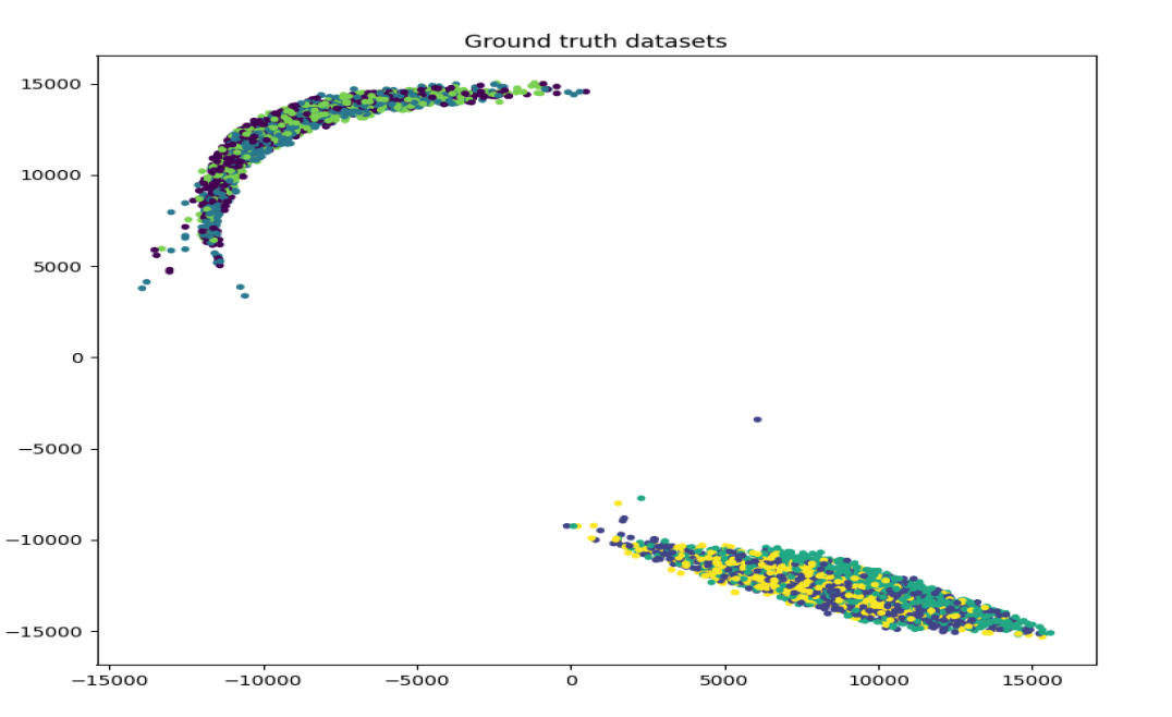
(a) Ground Truth

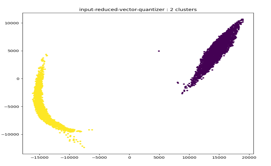
(b) Vector quantisation router

Figure 3: 2D projection of the hidden states of LLaMA2 on the ACRE i.i.d and o.o.d sets. The ground truth divides the samples as in Table 1 (text/symbolic i.i.d/o.o.d sets). The router shows the division into two domain-specific modules. The embedding space is divided into two main clusters that separate the text and symbolic inputs but the i.i.d and o.o.d sets are clustered together. The router follows the same clusters.

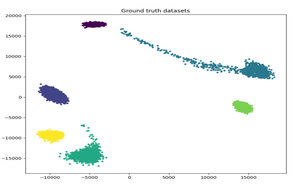
(c) Ground Truth

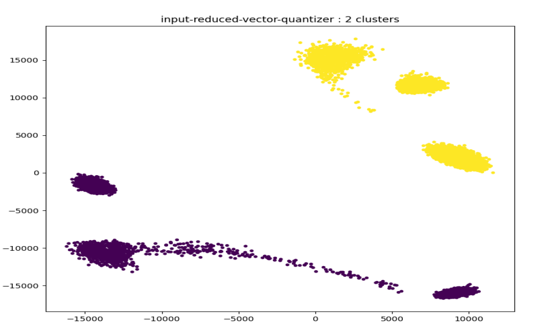
(d) Vector quantisation router

Figure 4: 2D projection of the hidden states of LLaMA2 on the RAVEN i.i.d and o.o.d sets. The characteristics are the same as in Figure 4. The embedding space is divided into six clusters separating text and symbolic inputs, and i.i.d and o.o.d sets. The router still divides the inputs between text and symbolic.

5.5 Continual Learning

We investigate the capacity of our model to be used in continual learning settings. Continual learning consists of training a model with continuous data streams or sets evolving over time, where the model acquires and accumulates knowledge incrementally. The main challenge lies in the catastrophic forgetting of the previous knowledge when gaining new information (Wang et al., 2023).

We study a simple scenario where we want our model to learn one new task after training on a previous task. We choose the scenario $ACRE\rightarrow RAVEN$ as RAVEN is more complicated to solve for an LLM, particularly the o.o.d sets. The results are shown in Table 3.

The table shows that the domain-invariant module can use general information extracted from ACRE to improve its performance on RAVEN, outperforming the baseline trained on RAVEN only. It suffers from the same forgetting problem as LLaMA2 but the domain-specific modules mitigate this issue. Their weights are not updated because the router does not activate them on RAVEN inputs, and their performance on ACRE is preserved. However, the aggregation process is hurt and leads to reduced performance on ACRE Text. In addition, due to the fixed number of centroids in our routing strategy, after training on ACRE, we must retrain the router with four centroids to include the two modules specialised in RAVEN. We discuss this limitation further in Section 6.

Table 3: Accuracy on the ACRE and RAVEN datasets when the model is trained on ACRE and RAVEN in a sequence. The first two rows show the results from Tables 1 and 2 when fine-tuned on a single dataset. ICLM is able to use the information from ACRE to improve its performance on RAVEN, outperforming the baseline trained on RAVEN only, while preserving more knowledge from the previous task than the base LLaMA2-7B. In particular, the accuracy of ACRE-Symbolic sets is almost untouched.

	ACRET		-Comp		-Sys		RAVENT		-Four		-In-Center
	Text	Symb	Text	Symb	Text	Symb	Text	Symb	Text	Symb	Text	Symb
ICLMACRE*	0.653	0.950	0.663	0.931	0.634	0.901	-	-	-	-	-	-
ICLMRAVEN*	-	-	-	-	-	-	1.000	0.980	0.703	0.703	0.515	0.228
${\scriptstyle ACRE\rightarrow RAVEN}$
ICLM* (ours)	0.089	0.901	0.119	0.931	0.050	0.871	1.000	0.990	0.772	0.772	0.833	0.248
ICLM-Invariant* (ours)	0.287	0.396	0.277	0.416	0.238	0.455	1.000	0.970	0.673	0.723	0.723	0.238
LLaMA2-7B*	0.079	0.376	0.149	0.386	0.089	0.426	0.980	0.772	0.634	0.554	0.584	0.069

6 Discussion and Limitations

The model proposed in this paper is constrained to work in a modular manner. All modules are sparsely connected at the level of the language modelling head. As shown in Section 4, the domain-specific modules are independent of each other if the Mutual Information with the domain-invariant module is infinitely close to zero. They behave as specialised Independent Causal Mechanisms. However, are the learned mechanisms useful for the task? Do they represent the correct causal mechanisms of the problem?

The causal graph built has a single level of interaction between the modules. Although it can represent a wide range of problems (requiring the composition of several independent reasoning processes), this simple graph does not describe the causal mechanisms behind these problems with great precision. Generating complex causal computation graphs tailored to the task at hand may improve performance, but this problem is out of the scope of this paper.

We conduct experiments on reasoning tasks to verify if inducing causal mechanisms (although simple) can yield increases in performance and generalisation. We aim not to outperform the state-of-the-art on the problems but to study whether the proposed mechanisms can yield such increases. We find that this is often the case. Our experiments demonstrate promising results in this direction, particularly for o.o.d reasoning and continual learning.

Nevertheless, we should highlight a few limitations of our work. The domain-specific modules are linked to a router centroid by key-value association. Therefore, the routing strategy assumes that all modules are identical and cannot take advantage of the specificities of each module when creating the centroid coordinates. For instance, when using fine-tuned domain-specific modules with an untrained router, each module will be randomly associated with one of the centroids. The necessity to retain the key-values dictionary can hinder the usability of the model for continual learning. Due to the unsupervised nature of the routing strategy, any clustering algorithm can be plugged. Although we focused on simple strategies in our work, more advanced clustering algorithms could capture more complex clusters, e.g. DBSCAN (Ester et al., 1996). Using clustering algorithms with an evolving number of clusters is another direction that could also be useful for continual learning.

In addition, training and fine-tuning Large Language Models has a high computational cost. Due to this high cost, we perform a single fine-tuning run per task and conduct experiments on this model.

7 Conclusion

Performing strong out-of-distribution reasoning is a challenging task, and despite their impressive performance on a wide range of problems, Large Language Models have not demonstrated this ability yet. Combining this popular model with causal models could help bridge this gap. This work has presented a modular architecture emulating Independent Causal Mechanisms in LLMs. To this end, we have introduced a routing mechanism and a regularisation process based on information theory. We show theoretically that the proposed model generates independent causal modules. We perform experiments on abstract and causal reasoning tasks in o.o.d and continual learning settings and obtain promising results, showing that these principles can increase strong reasoning and generalisation. In our future work, we will study the transfer of these abilities to other tasks. We will also experiment with larger models and investigate further the connection between causal routing and generalisation. Finally, we will work on building architectures representing more complex types of causal graphs.

Broader Impact

This paper presents work whose goal is to advance the field of Machine Learning. There are many potential societal consequences of our work, none which we feel must be specifically highlighted here.

Appendix A Supplement to the Theoretical Perspective

(a) Simplified temporal causal graph during training with no domain-invariant module.

(b) Simplified temporal causal graph $\mathcal{G}$. The graph is the same as Figure 2.

(c) Temporal causal graph with Information Minimisation loss added.

Figure 5: Causal graphs with and without domain-invariant module and Mutual Information minimisation loss. C is the input context. $H_{R}$, $H_{I}$, $H_{S_{n}}$, $H_{S}$ are the latent states of the router, domain-invariant, domain-specific and activated domain-specific (after router weighting) modules. For simplicity, we only show the state $H_{S_{n}}$ of the activated domain-specific module $n$. $Y$ and $Y_{true}$ are the output and true distributions. $W_{R}$, $W_{S_{n}}$ and $W_{I}$ are the trainable parameters of the modules. $\mathcal{L}_{Y}=\mathcal{L}_{o}+\alpha\cdot\mathcal{L}_{inv}+\beta\cdot\mathcal{L}_{dom}$ and $\mathcal{L}_{R}$ are the output and router losses. Black edges show the forward pass at step $\tau$. Blue dashed edges show the backward pass at step $\tau$. Red dotted edges illustrate the causal links between the forward and backward passes. For simplicity, we only show the step for the loss variables as they appear twice. All other variables are at step $\tau$.

In this section, we prove the assertions made in Section 4 of the main paper. We study under what conditions the following equations (repeated from Section 4) hold:

$$P(H_{R}|\mathbf{do}(H_{S_{n}}))=P(H_{R})~{}\forall n\in[1,N]$$ (10)

$$P(H_{R}|\mathbf{do}(H_{I}))=P(H_{R})$$ (11)

$$\begin{aligned} &P(H_{S_{n}}|\mathbf{do}(H_{S_{\hat{n}}}))=P(H_{S_{n}})\\ &~{}~{}~{}~{}~{}~{}\forall\hat{n}\in[1,N]\setminus\{n\}~{}\forall n\in[1,N]\end{aligned}$$ (12)

$$P(H_{I}|\mathbf{do}(H_{S_{n}}))=P(H_{I})~{}\forall n\in[1,N]$$ (13)

$H_{R}$, $H_{I}$ and $H_{S_{n}}~{}\forall n\in[1,N]$ are the respective representations generated by the router, domain-invariant and $N$ domain-specific modules.

The rules of do-calculus, defined in Pearl [1995], allow one to reduce interventional queries (with the $\mathbf{do}(\cdot)$ operator) to observational queries. We will only use the deletion of actions rule. A simplified rule is shown in Equation 14:

$$\begin{aligned} &P(Y|\mathbf{do}(X))=P(Y)\\ &\text{~{}~{}~{}~{}~{}if~{}}(Y\!\perp\!\!\!\perp X)_{\mathcal{G}_{\overline{X}}}\end{aligned}$$ (14)

$\mathcal{G}_{\overline{X}}$ represents the causal graph $\mathcal{G}$ with the incoming edges of $X$ removed.

Let us first address the causal relationships of the router. Equations 11 and 10 can be verified using the simplified causal graph in Figure 5. They are a direct application of rule 14. When removing the parents of $H_{S_{n}}$ or $H_{I}$, $H_{R}$ is d-separated [Pearl, 1988] from them: the backward path through $C$ is blocked and the forward path through $W_{R}$ is not connected to $H_{S_{n}}$ or $H_{I}$. This is due to the use of a separate loss function for training the router when using the vector quantisation routing strategy. One could notice that we do not represent the sum of losses of Equation 5. We omit it in the simplified graph. Its impact on the backward pass is incidental since each element can be optimised independently.

Let us now address the causal relationships of one activated domain-specific module $n$ with its counterparts (Equation 12). Again, under graph $\mathcal{G}_{\overline{H_{S_{\hat{n}}}}}$, $H_{S_{n}}$, the backward path through $C$ between is blocked. In addition, we make the assumption that only the module $n$ is activated and is connected to $Y$ as in Figure 5. This assumption is verified when using the vector quantisation routing strategy. As a consequence, the routing process $H_{S}$ can be decomposed into multiple subgraphs $H_{S_{n}}\xrightarrow{H_{R}}Y$ and $H_{S_{\overline{n}}}\not\xrightarrow{H_{R}}Y~{}\forall\overline{n}\in[1,N]\setminus\{n\}$, with $A\xrightarrow{H_{R}}B$ equivalent to having $A\rightarrow X\leftarrow H_{R}$ and $X\rightarrow B$. $A\not\xrightarrow{H_{R}}B$ removes the second link. Therefore, during the backward pass, there is only one link $\mathcal{L}_{Y}\rightarrow W_{S_{n}}\rightarrow H_{S_{n}}$ and no path to the other domain-specific modules $\overline{n}$. A last type of path can exist; here is an example: assuming a model with two domain-specific modules, $S_{0}$ and $S_{1}$, activated one after the other, the following path exists: $H_{S_{1}}\xrightarrow{H_{R}}Y_{\tau}\rightarrow\mathcal{L}_{Y_{\tau}}\rightarrow W_{I}\xrightarrow{C}H_{I}\rightarrow Y_{\tau+1}\rightarrow\mathcal{L}_{Y_{\tau+1}}\rightarrow W_{S_{2}}\xrightarrow{C}H_{S_{2}}$. There is a causal path forward path from $H_{S_{1}}$ to $H_{S_{2}}$. The path does not exist if there is no invariant module, and Equation 12 holds.

If an invariant module is part of the model, Equations 12 and 13 do not hold because of the path above: $H_{I}$ and $H_{S_{n}}$ are not independent in the causal graph $\mathcal{G}_{H_{S_{n}}}$. Independence is achieved by minimising the Mutual Information between $H_{I}$ and $H_{S_{n}}$, as discussed in the main paper.

Appendix B Additional Routing Strategies

In our main experiments, we use a simple routing strategy based on computing vector quantisation from Euclidean distance. In this section, we consider several additional routing strategies:

• K-Means Clustering

• Euclidean Distance Weighting

K-Means Clustering

This strategy computes the clusters using K-Means (Lloyd’s algorithm) [Lloyd, 1982]. We first learn the cluster centroids on the training set separately. Then, we fine-tune the other modules. Therefore, the clustering mechanism is independent of the gradient descent during fine-tuning, and the quality of the clusters with respect to the data distribution depends solely on the robustness of the clustering method. For efficiency reasons, we do not directly perform the clustering on the hidden states of the router module. Before clustering an input embedding, we project it to a more dense space with fewer dimensions (typically 64). We apply Multidimensional Scaling with the SMACOF algorithm [Borg and Groenen, 2005]. The algorithm requires us to provide a base of the input space to perform the projection. We span the space using a random set of vectors from the training space. Because the distribution is skewed, we do not have a warranty to build a base. To remain computation-efficient, we sample $8\times M$ vectors with $M$ the dimensionality of the reduced space.

Euclidean Distance Weighting

This strategy differs from the other ones as it does not use vector quantisation. Instead, we compute the Euclidean distance between the embeddings and the centroid coordinates (randomly initialised) and use softmin to convert the distances into continuous weights between zero and one. The lower the distance between the embedding and a centroid, the higher the weight the corresponding domain-specific module will have on the output. Consequently, with this method, all domain-specific modules are always activated. This operation is differentiable and is the closest to the routing process of Mixture-of-Expert models like the Switch Transformer [Fedus et al., 2022b]. This method does not follow the causal structure discussed in Section 4. Instead, it uses the output loss to update the centroid coordinates.

The results obtained with these two routing strategies are provided in Appendix D.3.

Appendix C Additional Aggregation Schemes

In this section, we describe two additional aggregation schemes between the domain-invariant and domain-specific modules. Instead of using a shared language modelling head, we propose to use a separate head for each module and combine their outputs at the end by a weighted sum. This method tackles the issue of prioritised modules (e.g. one module being overused at the expense of the others). However, the information from the modules is not linearly combined but added separately, reducing expressivity.

We want to bound the output of each model such that it influences the final prediction by a pre-determined factor (given by the router output for the domain-specific modules and provided as a hyperparameter for the domain-invariant module). Each module outputs unbounded logits. The lack of bounds prevents them from directly multiplying the logits by their weighting factor and summing them together. Indeed, one module could overcome the weighting by increasing the magnitude of its logits. We consider two combination schemes: in the logit space and in the probability space.

Combination in the logit space

The aggregation scheme in the logit space is very similar to the one performed in the latent space in the main paper. We first perform a shared batch normalisation [Ioffe and Szegedy, 2015] between the modules to overcome the unbounded issue in the logit space. For a batch of size $|\mathcal{B}|$, one domain-specific active module and one domain-invariant module, batch normalisation is operated on $2\times|\mathcal{B}|$ samples. We attribute a weight $w_{I}$ to the domain-invariant module as a hyperparameter and $w_{S_{n}}=r_{n}\cdot(1-w_{I})$ to the domain-specific module, with $r_{n}$ the weight given by the router. After normalisation, We multiply each logit value by its corresponding weight and sum them together.

Combination in the probability space

Each module outputs unbounded logits, so we first convert each output into normalised probabilities (that sum to one). We then perform the weighting in each probability space before converting them back to logits (shown in Equation 15). Finally, the outputs from all modules are summed together (shown in Equation 16). The final probabilities are shown in Equation 17.

$$\widetilde{l_{a}}(Y|c) =\log\Big{(}\dfrac{1-w_{a}}{2}+w_{a}\cdot P_{a}(Y|c))\Big{)}+\log(B_{a})$$ (15)

$$l(Y|c) =\widetilde{l_{I}}(Y|c)+\sum\limits_{n\in[1,N]}\widetilde{l_{S_{n}}}(Y|c)$$ (16)

$$P(Y|c) =\sigma(l(Y|c))$$ (17)

$c$ is the input context. $P(Y|c)$ is the final output distribution between all words $Y$, obtained using softmax normalisation $\sigma$ on the output logits $l(Y|c)$. The output logits are obtained by summing the weighted logits of the domain-invariant module $\widetilde{l_{I}}(Y|c)$ and all domain-specific modules $\widetilde{l_{S_{n}}}(Y|c)$. Equation 15 shows the weighting process for all modules ($a\in\{I,S_{1},\dots,S_{N}\}$). The weight $w_{I}$ is a hyperparameter set prior to training. The weights $w_{S_{n}}\forall~{}n\in[1,N]$ combine the weight $w_{I}$ with the router weights $r_{n}$: $w_{S_{n}}=r_{n}\cdot(1-w_{I})$. $B_{a}$ is a normalisation term that ensures the conversion function between probabilities and logits is invertible.

The results obtained with these two aggregation schemes are provided in Appendix D.4.

Appendix D Additional Experiments

D.1 Evolution of the Mutual Information Across Training

To ensure the independence between the domain-specific and domain-invariant modules, we minimise the mutual Information between them. Figure 7 shows the evolution of Mutual Information during training. We observe that it quickly decreases to reach below $0,0001$. Figure 7 shows the same loss for the variants using aggregation in the logit and probability spaces. Unlike for the main model, we observe small spikes in the loss after $100$ training steps. The aggregation scheme that uses a shared language modelling head (our default) seems more stable during training.

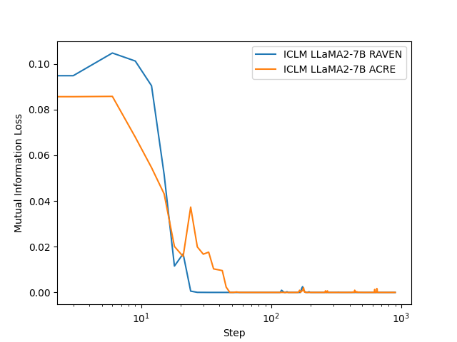
Figure 6: Evolution of the Mutual Information loss during training on ACRE and RAVEN. The x-axis corresponds to the number of training steps and is shown in the log scale.

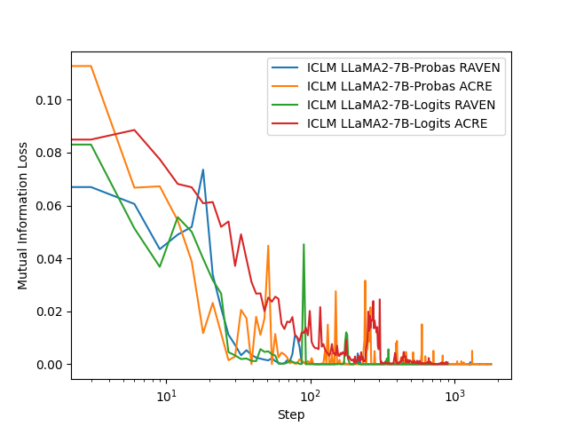
Figure 7: Evolution of the Mutual Information loss during training of variants with probability and logits aggregation on ACRE and RAVEN. The x-axis corresponds to the number of training steps and is shown in the log scale.

D.2 Routing Alignment and Visualisation

We study the module attribution performed by the router more deeply. Table 4 shows the alignment between the two domain-specific modules. We first observe that the division is mainly syntactic: each module specialises towards one type of input format, either text or symbolic. It aligns perfectly with the dataset.

Table 4: Alignment between modules and formats in the ACRE dataset. Each column shows the proportion of activation for each module for a given dataset. Each module specialises perfectly to one dataset.

	ACRE		-Comp		-Sys
	Text	Symb	Text	Symb	Text	Symb
$n=0$	0.0	1.0	0.0	1.0	0.0	1.0
$n=1$	1.0	0.0	1.0	0.0	1.0	0.0

Figures 8, 9, 10 and 11 show visualisations of the clusters in a 2D space. Figures 8 and 9 show the i.i.d and o.o.d sets of ACRE. Figures 10 and 11 show the i.i.d and o.o.d sets of RAVEN. As in the main paper, the projection is made using Multidimensional Scaling (MDS) [Borg and Groenen, 2005]. For illustration purposes, we observe the clusters formed by the K-Means method for $N=4$ modules. We also observe the clusters formed from the penultimate hidden states of the router. As discussed above and in the main paper, there is a clear division between text and symbolic embeddings, but the o.o.d sets are not well separated in ACRE while they are in RAVEN. This division (and absence of division) is also present in the previous hidden states, although the separation is less obvious: all embeddings tend to align to a single axis.

We want to study the router’s behaviour further when faced with a diverse set of input data. To this end, we feed six different datasets to the model: the i.i.d text and symbolic sets of ACRE and RAVEN, PVR [Zhang et al., 2021b] and ARC [Chollet, 2019] datasets. The visualisations are in Figure 12. Overall, the datasets are well separated but have different shapes. While some form dense amalgamates, others spread in the latent space. The observations from ACRE and RAVEN suggest that the distance in the embedding space between a module cluster and an input can be an indicator of the module’s performance on the input. The o.o.d sets of ACRE are merged in the latent space, and the model maintains accuracy across the sets. In parallel, the o.o.d sets of RAVEN are separated by clear boundaries, and the accuracy drops as the distance with the i.i.d set increases. Experiments on a larger scale are needed to validate or invalidate the hypothesis and discriminate the true causes responsible for this behaviour from spurious correlations.

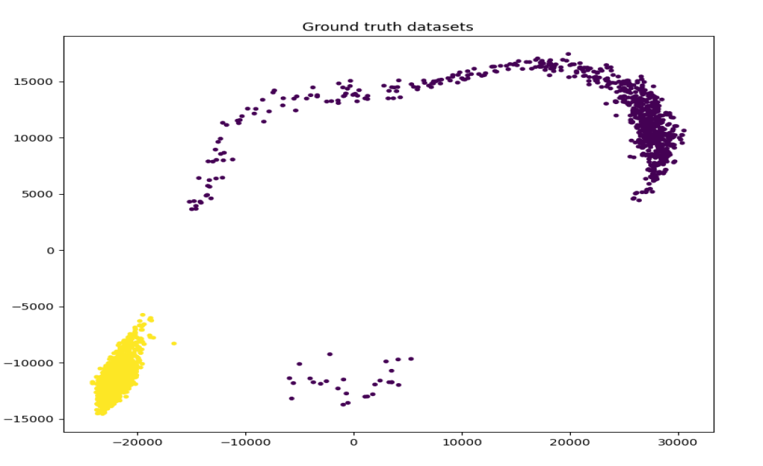
(a) Ground Truth ($l=-1$)

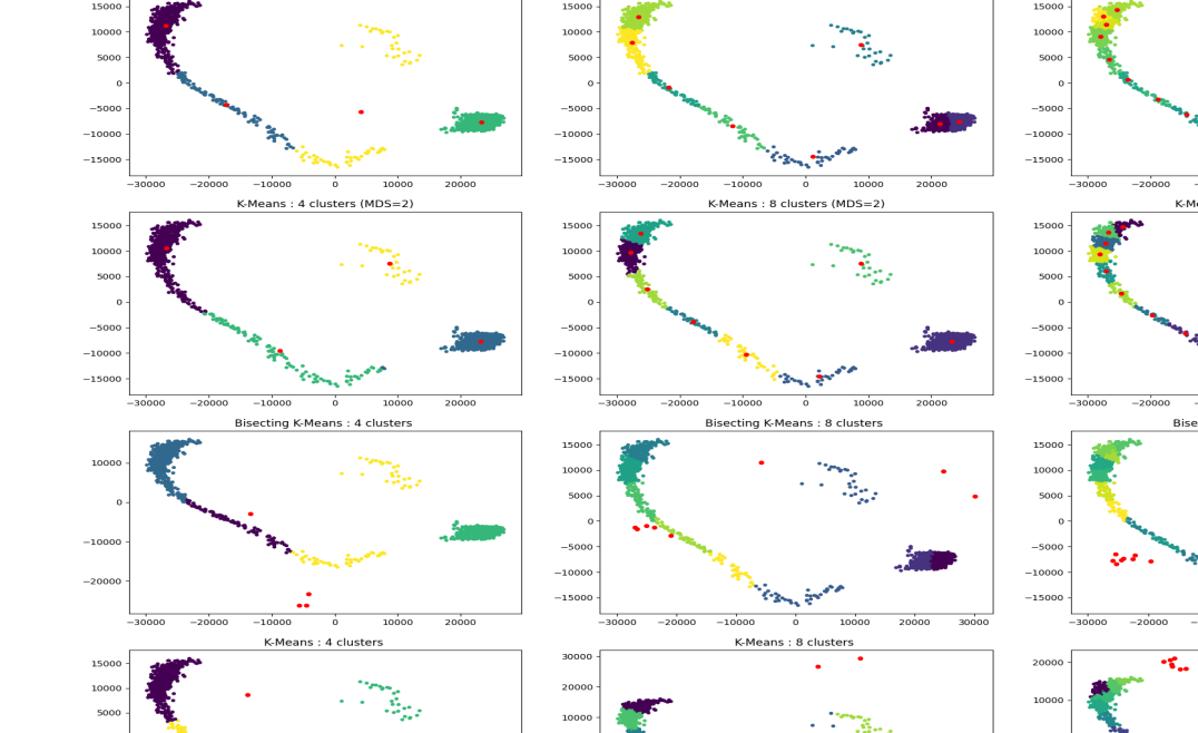
(b) K-Means ($l=-1$)

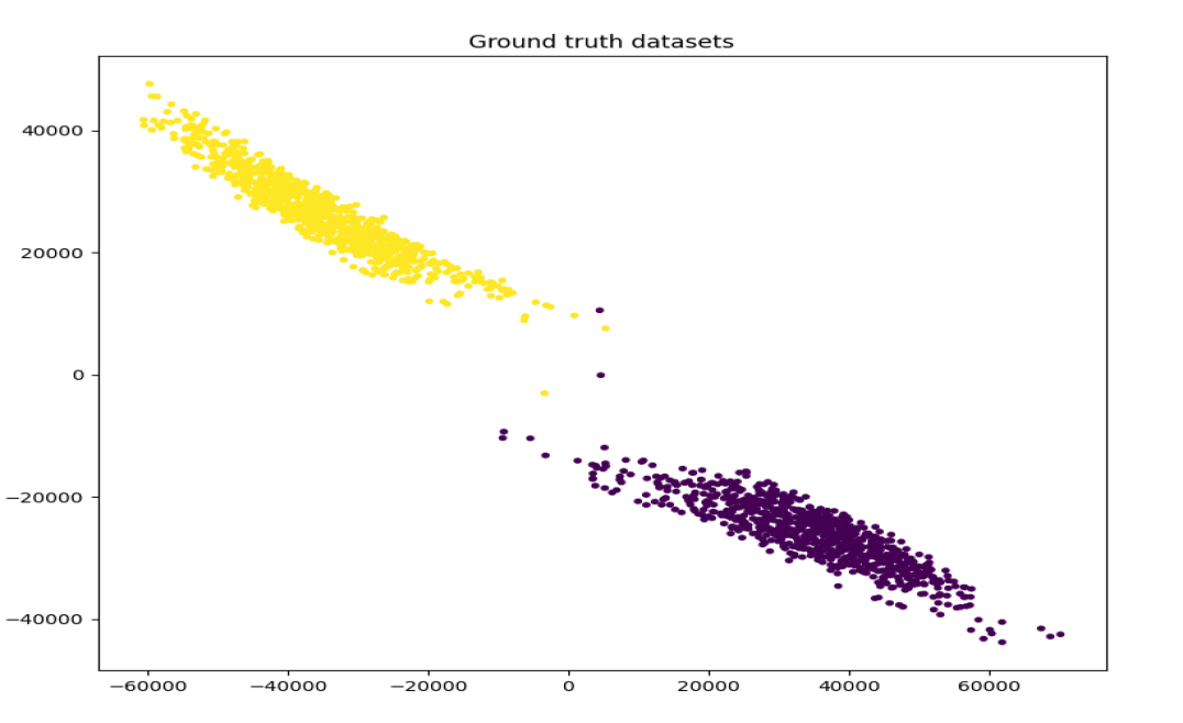
(c) Ground Truth ($l=-2$)

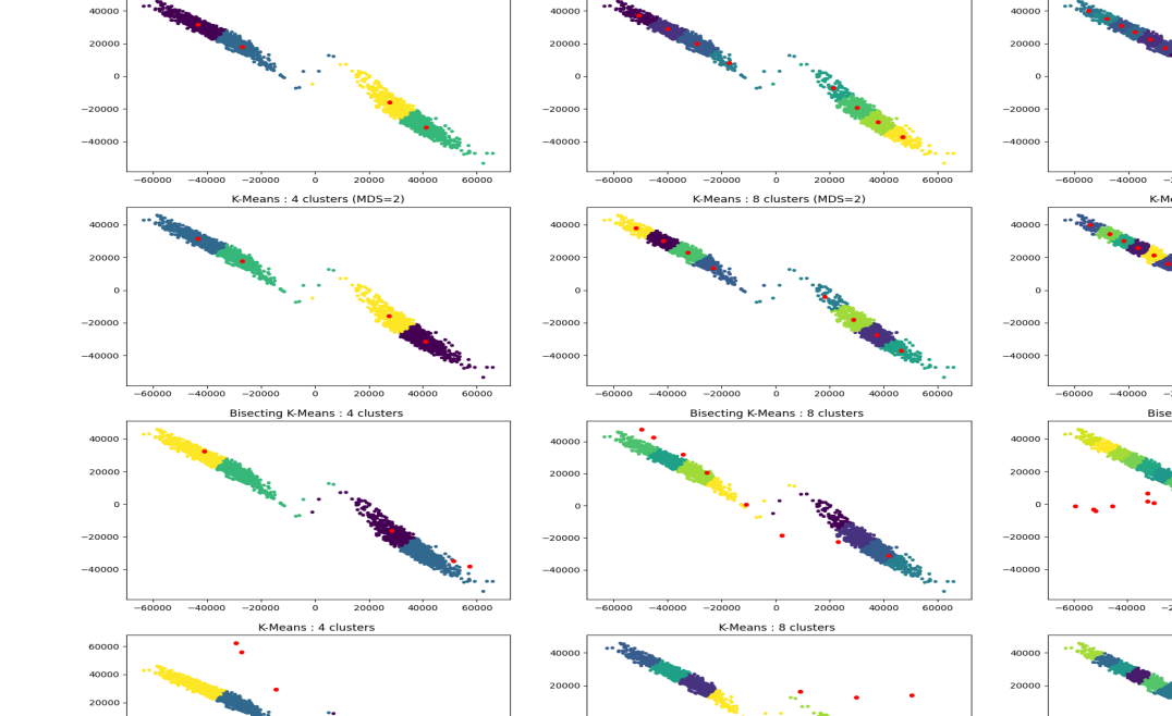
(d) K-Means ($l=-2$)

Figure 8: Clusters formed from the hidden states of LLaMA2 on the ACRE training sets. The visualisations contain the last two levels ($l$) of hidden layers. The ground truth shows the true splits (text/symbolic). The learned clusters use 4 centroids.

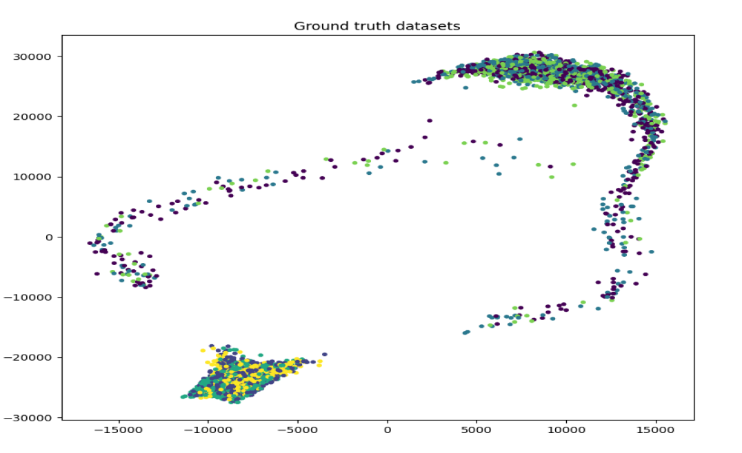
(a) Ground Truth ($l=-1$)

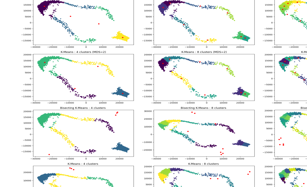
(b) K-Means ($l=-1$)

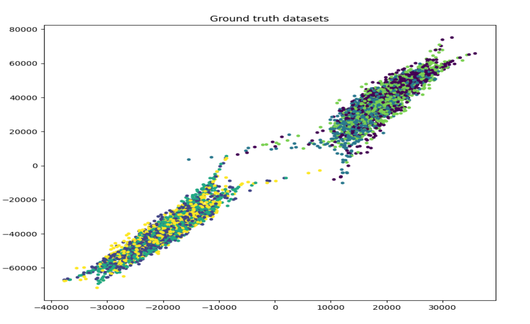
(c) Ground Truth ($l=-2$)

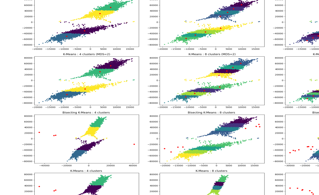
(d) K-Means ($l=-2$)

Figure 9: Clusters formed from the hidden states of LLaMA2 on the ACRE o.o.d sets. The visualisations contain the last two levels ($l$) of hidden layers. The ground truth shows the true splits (text/symbolic/o.o.d splits). The learned clusters use 4 centroids.

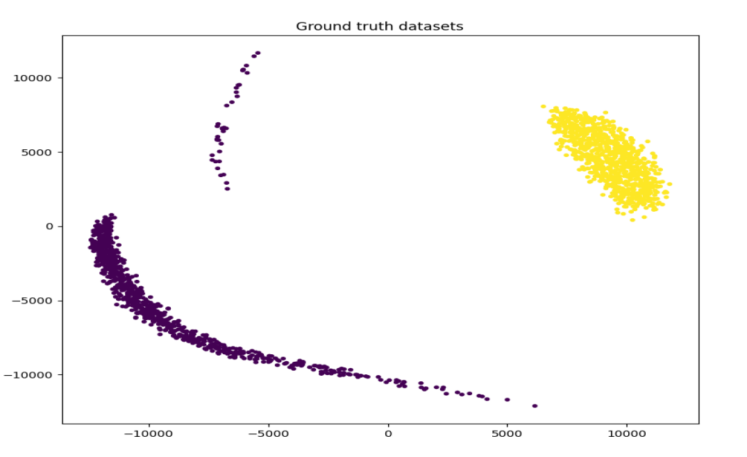
(a) Ground Truth ($l=-1$)

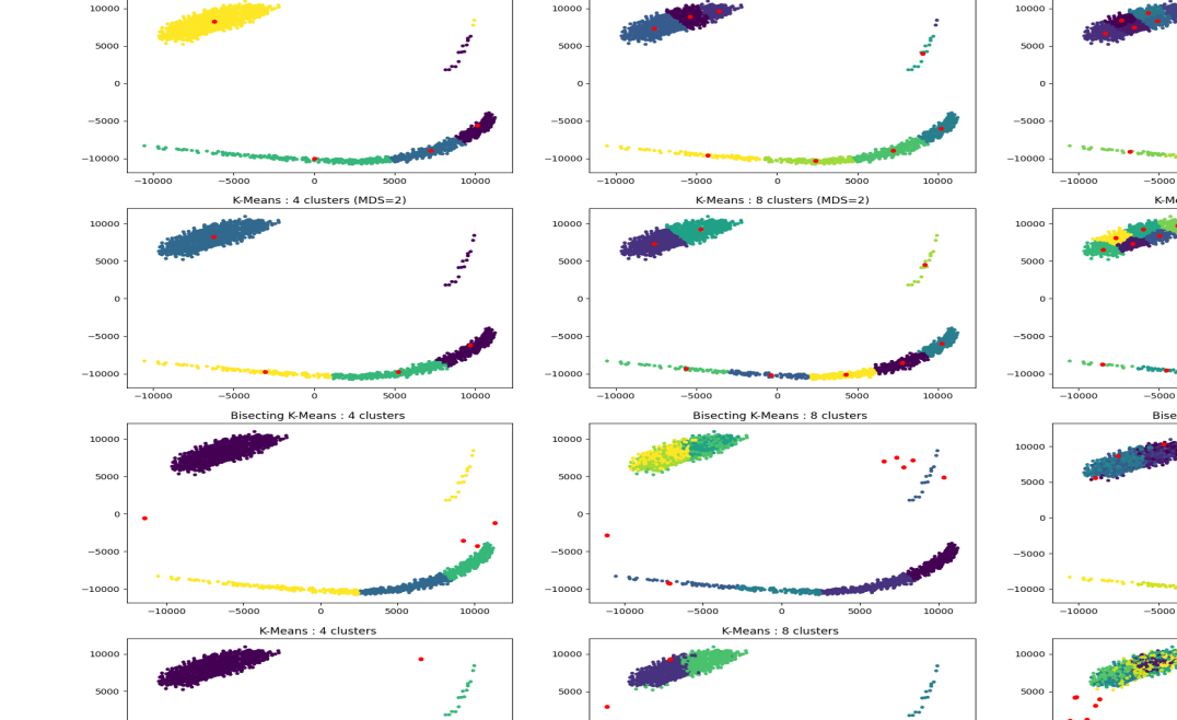
(b) K-Means ($l=-1$)

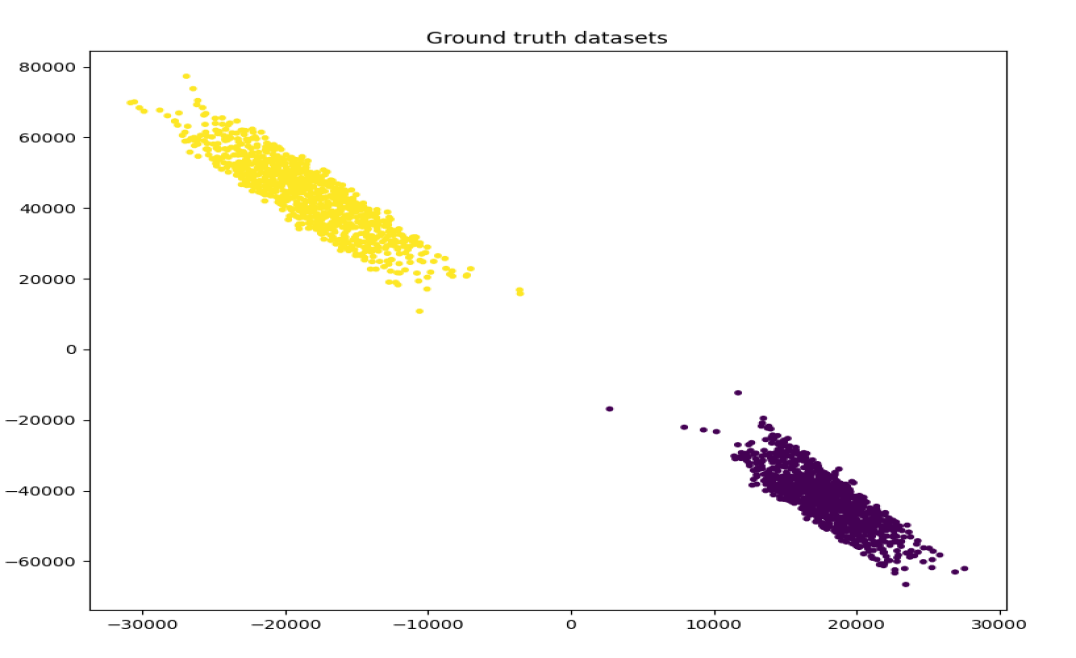
(c) Ground Truth ($l=-2$)

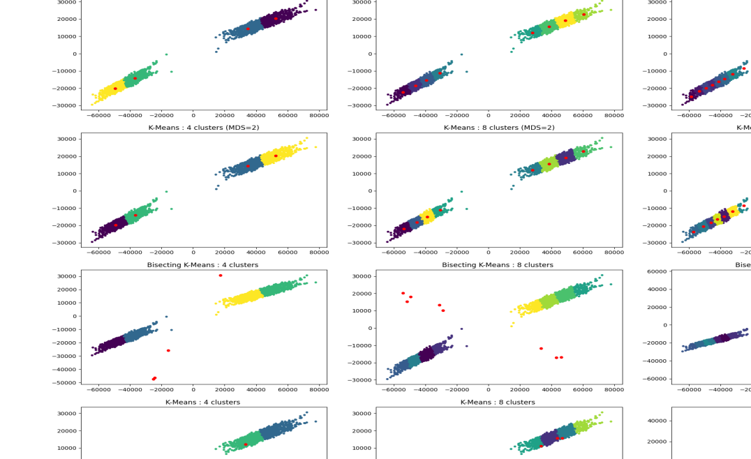
(d) K-Means ($l=-2$)

Figure 10: Clusters formed from the hidden states of LLaMA2 on the RAVEN training sets. The visualisations contain the last two levels ($l$) of hidden layers. The ground truth shows the true splits (text/symbolic). The learned clusters use 4 centroids.

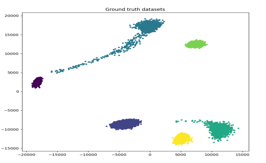
(a) Ground Truth ($l=-1$)

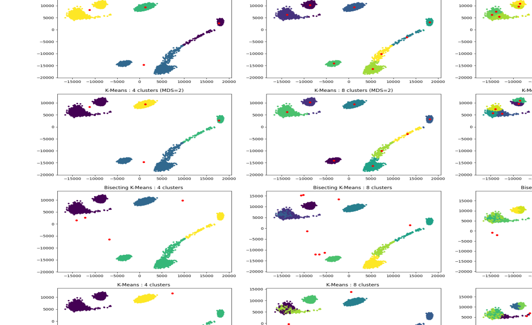
(b) K-Means ($l=-1$)

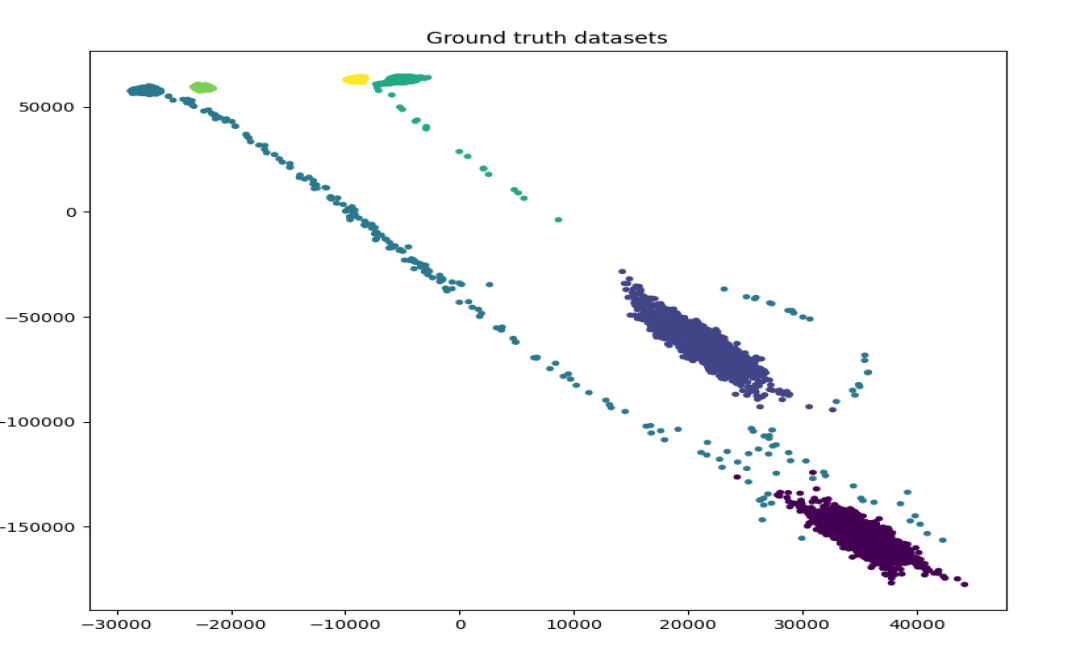
(c) Ground Truth ($l=-2$)

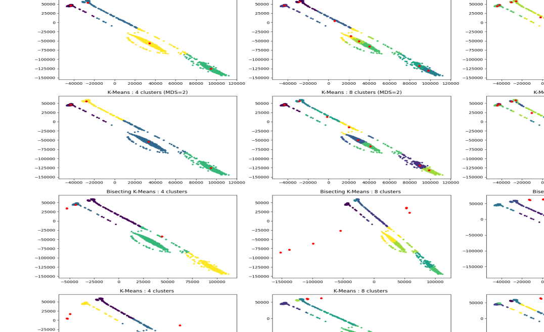
(d) K-Means ($l=-2$)

Figure 11: Clusters formed from the hidden states of LLaMA2 on the RAVEN o.o.d sets. The visualisations contain the last two levels ($l$) of hidden layers. The ground truth shows the true splits (text/symbolic). The learned clusters use 4 centroids.

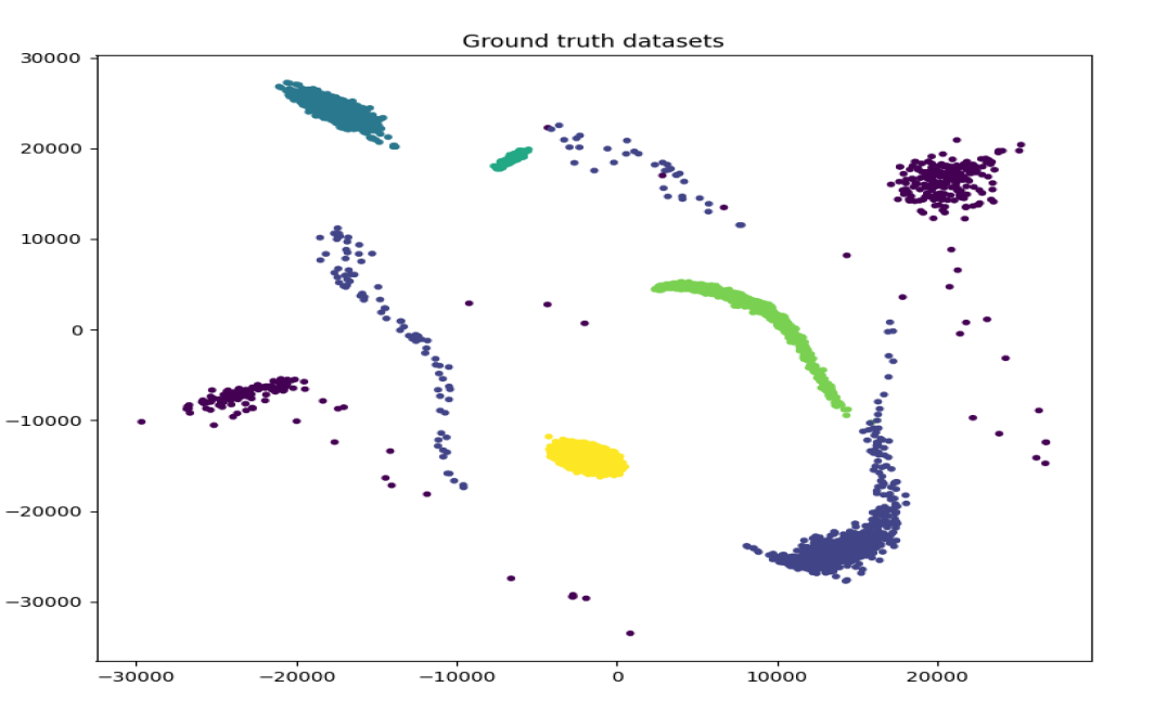
(a) Ground Truth ($l=-1$)

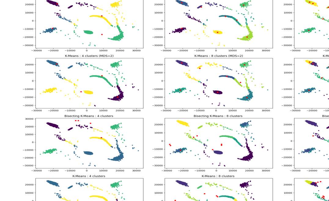
(b) K-Means ($l=-1$)

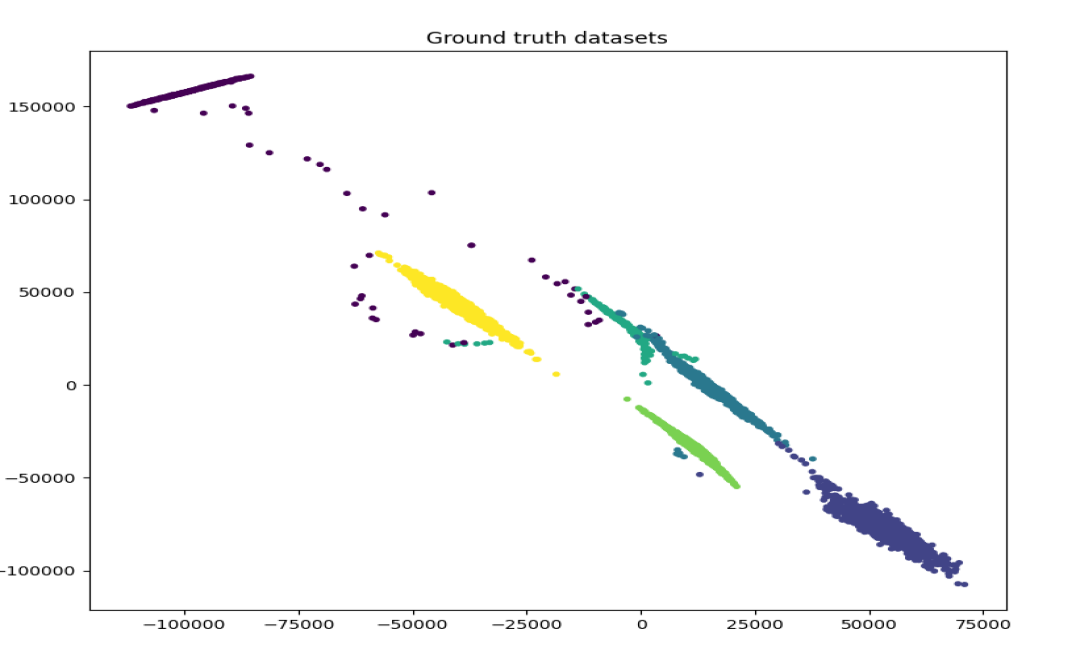
(c) Ground Truth ($l=-2$)

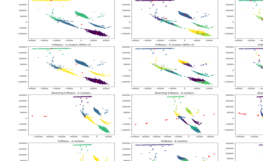
(d) K-Means ($l=-2$)

Figure 12: Clusters formed from the hidden states of LLaMA2 on the training sets of ACRE, ARC, PVR and RAVEN. The visualisations contain the last two levels ($l$) of hidden layers. The ground truth shows the true splits between each dataset. The learned clusters use 4 centroids.

D.3 Variations of the Routing Strategy

We perform additional experiments on ACRE and RAVEN datasets using the routing strategies introduced in Appendix B: K-Means and weighting. Tables 5 and 6 show the results.

Table 5: Accuracy on the ACRE i.i.d and o.o.d test sets. Datasets are represented in columns, and models in rows. ICLM is trained on text and symbolic i.i.d training sets. Models with a ^∗ indicate that the results are introduced in this paper. The best model is shown in bold.

	ACRE		-o.o.d-Comp		-o.o.d-Sys
	Text	Symb	Text	Symb	Text	Symb
ICLM* (ours)	0.653	0.950	0.663	0.931	0.634	0.901
ICLM-Weighted* (ours)	0.812	0.921	0.802	0.960	0.842	0.970
ICLM-K-Means* (ours)	0.901	0.881	0.911	0.911	0.891	0.921

Table 6: Accuracy on the RAVEN i.i.d and o.o.d test sets. The characteristics are the same as in Table 5.

	RAVEN		-o.o.d-Four		-o.o.d-In-Center
	Text	Symb	Text	Symb	Text	Symb
ICLM* (ours)	1.000	0.980	0.703	0.703	0.515	0.228
ICLM-Weighted* (ours)	1.000	1.000	0.743	0.703	0.653	0.248
ICLM-K-Means* (ours)	1.000	1.000	0.634	0.673	0.515	0.287

The alternative routing strategies achieve similar and sometimes superior performance than the base ICLM model. As observed in the previous section, the router creates well-defined clusters that the K-Means and Euclidean distance vector quantisation strategies tend to follow. No explicit differentiation of the routing process can be observed from the visualisations. The difference in performance may lie in the optimisation process. K-Means does not backpropagate information to the router; weighting backpropagates from the output loss, and vector quantisation backpropagates from a secondary loss.

D.4 Variations of the Aggregation Scheme

We perform additional experiments on ACRE and RAVEN datasets using the aggregation schemes introduced in Appendix C: in the logit and probability spaces. Tables 5 and 6 show the results.

Table 7: Accuracy on the ACRE i.i.d and o.o.d test sets.

	ACRE		-o.o.d-Comp		-o.o.d-Sys
	Text	Symb	Text	Symb	Text	Symb
ICLM* (ours)	0.653	0.950	0.663	0.931	0.634	0.901
ICLM-Logits* (ours)	0.842	0.950	0.881	0.901	0.901	0.921
ICLM-Probas* (ours)	0.921	0.950	0.832	0.921	0.891	0.931

Table 8: Accuracy on the RAVEN i.i.d and o.o.d test sets.

	RAVEN		-o.o.d-Four		-o.o.d-In-Center
	Text	Symb	Text	Symb	Text	Symb
ICLM* (ours)	1.000	0.980	0.703	0.703	0.515	0.228
ICLM-Logits* (ours)	1.000	0.990	0.644	0.713	0.703	0.268
ICLM-Probas* (ours)	0.802	0.931	0.614	0.624	0.495	0.297

As per the routing strategies, the alternative aggregation schemes achieve similar and sometimes superior performance than the base ICLM model. No scheme is systematically better than the others. These results show that less expressive aggregation methods, i.e. weighted sums, can perform similarly to trained dense layers on abstract and causal reasoning tasks.

References

- Austin [2011] Peter C. Austin. An introduction to propensity score methods for reducing the effects of confounding in observational studies. Multivariate Behavioral Research, 46(3):399–424, 2011. PMID: 21818162.
- Bao et al. [2022] Hangbo Bao, Li Dong, Songhao Piao, and Furu Wei. Beit: BERT pre-training of image transformers. In The Tenth International Conference on Learning Representations, ICLR 2022, Virtual Event, April 25-29, 2022. OpenReview.net, 2022.
- Bao et al. [2023] Qiming Bao, Gaël Gendron, Alex Yuxuan Peng, Wanjun Zhong, Neset Tan, Yang Chen, Michael Witbrock, and Jiamou Liu. A systematic evaluation of large language models on out-of-distribution logical reasoning tasks. CoRR, abs/2310.09430, 2023.
- Bareinboim et al. [2022] Elias Bareinboim, Juan D. Correa, Duligur Ibeling, and Thomas Icard. On pearl’s hierarchy and the foundations of causal inference. In Hector Geffner, Rina Dechter, and Joseph Y. Halpern, editors, Probabilistic and Causal Inference: The Works of Judea Pearl, volume 36 of ACM Books, pages 507–556. ACM, 2022.
- Borg and Groenen [2005] Ingwer Borg and Patrick JF Groenen. Modern multidimensional scaling: Theory and applications. Springer Science & Business Media, 2005.
- Brown et al. [2020] Tom B. Brown, Benjamin Mann, Nick Ryder, Melanie Subbiah, Jared Kaplan, Prafulla Dhariwal, Arvind Neelakantan, Pranav Shyam, Girish Sastry, Amanda Askell, Sandhini Agarwal, Ariel Herbert-Voss, Gretchen Krueger, Tom Henighan, Rewon Child, Aditya Ramesh, Daniel M. Ziegler, Jeffrey Wu, Clemens Winter, Christopher Hesse, Mark Chen, Eric Sigler, Mateusz Litwin, Scott Gray, Benjamin Chess, Jack Clark, Christopher Berner, Sam McCandlish, Alec Radford, Ilya Sutskever, and Dario Amodei. Language models are few-shot learners. In Proceedings of the 34th International Conference on Neural Information Processing Systems, NIPS’20, Red Hook, NY, USA, 2020. Curran Associates Inc.
- Bubeck et al. [2023] Sébastien Bubeck, Varun Chandrasekaran, Ronen Eldan, Johannes Gehrke, Eric Horvitz, Ece Kamar, Peter Lee, Yin Tat Lee, Yuanzhi Li, Scott Lundberg, Harsha Nori, Hamid Palangi, Marco Tulio Ribeiro, and Yi Zhang. Sparks of artificial general intelligence: Early experiments with gpt-4. March 2023.
- Chollet [2019] François Chollet. On the measure of intelligence. CoRR, abs/1911.01547, 2019.
- Clark et al. [2022] Aidan Clark, Diego de Las Casas, Aurelia Guy, Arthur Mensch, Michela Paganini, Jordan Hoffmann, Bogdan Damoc, Blake A. Hechtman, Trevor Cai, Sebastian Borgeaud, George van den Driessche, Eliza Rutherford, Tom Hennigan, Matthew J. Johnson, Albin Cassirer, Chris Jones, Elena Buchatskaya, David Budden, Laurent Sifre, Simon Osindero, Oriol Vinyals, Marc’Aurelio Ranzato, Jack W. Rae, Erich Elsen, Koray Kavukcuoglu, and Karen Simonyan. Unified scaling laws for routed language models. In Kamalika Chaudhuri, Stefanie Jegelka, Le Song, Csaba Szepesvári, Gang Niu, and Sivan Sabato, editors, International Conference on Machine Learning, ICML 2022, 17-23 July 2022, Baltimore, Maryland, USA, volume 162 of Proceedings of Machine Learning Research, pages 4057–4086. PMLR, 2022.
- Ester et al. [1996] Martin Ester, Hans-Peter Kriegel, Jörg Sander, and Xiaowei Xu. A density-based algorithm for discovering clusters in large spatial databases with noise. In kdd, volume 96, pages 226–231, 1996.
- Fedus et al. [2022a] William Fedus, Jeff Dean, and Barret Zoph. A review of sparse expert models in deep learning. CoRR, abs/2209.01667, 2022.
- Fedus et al. [2022b] William Fedus, Barret Zoph, and Noam Shazeer. Switch transformers: Scaling to trillion parameter models with simple and efficient sparsity. J. Mach. Learn. Res., 23:120:1–120:39, 2022.
- Gendron et al. [2023a] Gaël Gendron, Qiming Bao, Michael Witbrock, and Gillian Dobbie. Large language models are not abstract reasoners. CoRR, abs/2305.19555, 2023.
- Gendron et al. [2023b] Gaël Gendron, Michael Witbrock, and Gillian Dobbie. Disentanglement of latent representations via causal interventions. In Proceedings of the Thirty-Second International Joint Conference on Artificial Intelligence, IJCAI 2023, 19th-25th August 2023, Macao, SAR, China, pages 3239–3247. ijcai.org, 2023.
- Gendron et al. [2023c] Gaël Gendron, Michael Witbrock, and Gillian Dobbie. A survey of methods, challenges and perspectives in causality. CoRR, abs/2302.00293, 2023.
- Goyal and Bengio [2020] Anirudh Goyal and Yoshua Bengio. Inductive biases for deep learning of higher-level cognition. CoRR, abs/2011.15091, 2020.
- Goyal et al. [2021] Anirudh Goyal, Alex Lamb, Jordan Hoffmann, Shagun Sodhani, Sergey Levine, Yoshua Bengio, and Bernhard Schölkopf. Recurrent independent mechanisms. In 9th International Conference on Learning Representations, ICLR 2021, Virtual Event, Austria, May 3-7, 2021. OpenReview.net, 2021.
- Gururangan et al. [2022] Suchin Gururangan, Mike Lewis, Ari Holtzman, Noah A. Smith, and Luke Zettlemoyer. Demix layers: Disentangling domains for modular language modeling. In Marine Carpuat, Marie-Catherine de Marneffe, and Iván Vladimir Meza Ruíz, editors, Proceedings of the 2022 Conference of the North American Chapter of the Association for Computational Linguistics: Human Language Technologies, NAACL 2022, Seattle, WA, United States, July 10-15, 2022, pages 5557–5576. Association for Computational Linguistics, 2022.
- Hochreiter and Schmidhuber [1997] Sepp Hochreiter and Jürgen Schmidhuber. Long short-term memory. Neural Comput., 9(8):1735–1780, 1997.
- Hu et al. [2022] Edward J. Hu, Yelong Shen, Phillip Wallis, Zeyuan Allen-Zhu, Yuanzhi Li, Shean Wang, Lu Wang, and Weizhu Chen. Lora: Low-rank adaptation of large language models. In The Tenth International Conference on Learning Representations, ICLR 2022, Virtual Event, April 25-29, 2022. OpenReview.net, 2022.
- Ioffe and Szegedy [2015] Sergey Ioffe and Christian Szegedy. Batch normalization: Accelerating deep network training by reducing internal covariate shift. In Francis R. Bach and David M. Blei, editors, Proceedings of the 32nd International Conference on Machine Learning, ICML 2015, Lille, France, 6-11 July 2015, volume 37 of JMLR Workshop and Conference Proceedings, pages 448–456. JMLR.org, 2015.
- Jiang et al. [2024] Albert Q. Jiang, Alexandre Sablayrolles, Antoine Roux, Arthur Mensch, Blanche Savary, Chris Bamford, Devendra Singh Chaplot, Diego de Las Casas, Emma Bou Hanna, Florian Bressand, Gianna Lengyel, Guillaume Bour, Guillaume Lample, Lélio Renard Lavaud, Lucile Saulnier, Marie-Anne Lachaux, Pierre Stock, Sandeep Subramanian, Sophia Yang, Szymon Antoniak, Teven Le Scao, Théophile Gervet, Thibaut Lavril, Thomas Wang, Timothée Lacroix, and William El Sayed. Mixtral of experts. CoRR, abs/2401.04088, 2024.
- Jin et al. [2023] Zhijing Jin, Jiarui Liu, Zhiheng Lyu, Spencer Poff, Mrinmaya Sachan, Rada Mihalcea, Mona T. Diab, and Bernhard Schölkopf. Can large language models infer causation from correlation? CoRR, abs/2306.05836, 2023.
- Kreer [1957] J. Kreer. A question of terminology. IRE Transactions on Information Theory, 3(3):208–208, 1957.
- Kullback and Leibler [1951] Solomon Kullback and Richard A Leibler. On information and sufficiency. The annals of mathematical statistics, 22(1):79–86, 1951.
- Liu et al. [2023] Hanmeng Liu, Ruoxi Ning, Zhiyang Teng, Jian Liu, Qiji Zhou, and Yue Zhang. Evaluating the logical reasoning ability of chatgpt and GPT-4. CoRR, abs/2304.03439, 2023.
- Lloyd [1982] Stuart Lloyd. Least squares quantization in pcm. IEEE transactions on information theory, 28(2):129–137, 1982.
- Loshchilov and Hutter [2019] Ilya Loshchilov and Frank Hutter. Decoupled weight decay regularization. In 7th International Conference on Learning Representations, ICLR 2019, New Orleans, LA, USA, May 6-9, 2019. OpenReview.net, 2019.
- Melnychuk et al. [2022] Valentyn Melnychuk, Dennis Frauen, and Stefan Feuerriegel. Causal transformer for estimating counterfactual outcomes. In Kamalika Chaudhuri, Stefanie Jegelka, Le Song, Csaba Szepesvári, Gang Niu, and Sivan Sabato, editors, International Conference on Machine Learning, ICML 2022, 17-23 July 2022, Baltimore, Maryland, USA, volume 162 of Proceedings of Machine Learning Research, pages 15293–15329. PMLR, 2022.
- Mittal et al. [2022] Sarthak Mittal, Yoshua Bengio, and Guillaume Lajoie. Is a modular architecture enough? In Sanmi Koyejo, S. Mohamed, A. Agarwal, Danielle Belgrave, K. Cho, and A. Oh, editors, Advances in Neural Information Processing Systems 35: Annual Conference on Neural Information Processing Systems 2022, NeurIPS 2022, New Orleans, LA, USA, November 28 - December 9, 2022, 2022.
- Paluš et al. [2001] Milan Paluš, Vladimír Komárek, Zbyněk Hrnčíř, and Katalin Štěrbová. Synchronization as adjustment of information rates: Detection from bivariate time series. Physical Review E, 63(4):046211, 2001.
- Pearl [1988] Judea Pearl. Probabilistic reasoning in intelligent systems: networks of plausible inference. Morgan kaufmann, 1988.
- Pearl [1995] Judea Pearl. Causal diagrams for empirical research. Biometrika, 82(4):669–688, 1995.
- Pearl [2009] Judea Pearl. Causality. Cambridge university press, 2009.
- Peters et al. [2017] Jonas Peters, Dominik Janzing, and Bernhard Schölkopf. Elements of causal inference: foundations and learning algorithms. The MIT Press, 2017.
- Ramesh et al. [2021] Aditya Ramesh, Mikhail Pavlov, Gabriel Goh, Scott Gray, Chelsea Voss, Alec Radford, Mark Chen, and Ilya Sutskever. Zero-shot text-to-image generation. In Marina Meila and Tong Zhang, editors, Proceedings of the 38th International Conference on Machine Learning, ICML 2021, 18-24 July 2021, Virtual Event, volume 139 of Proceedings of Machine Learning Research, pages 8821–8831. PMLR, 2021.
- Raven [1938] John C Raven. Raven standard progressive matrices. Journal of Cognition and Development, 1938.
- Schölkopf et al. [2021] Bernhard Schölkopf, Francesco Locatello, Stefan Bauer, Nan Rosemary Ke, Nal Kalchbrenner, Anirudh Goyal, and Yoshua Bengio. Towards causal representation learning. CoRR, abs/2102.11107, 2021.
- Schreiber [2000] Thomas Schreiber. Measuring information transfer. Physical review letters, 85(2):461, 2000.
- Shannon [1948] Claude Elwood Shannon. A mathematical theory of communication. The Bell system technical journal, 27(3):379–423, 1948.
- Touvron et al. [2023a] Hugo Touvron, Thibaut Lavril, Gautier Izacard, Xavier Martinet, Marie-Anne Lachaux, Timothée Lacroix, Baptiste Rozière, Naman Goyal, Eric Hambro, Faisal Azhar, Aurélien Rodriguez, Armand Joulin, Edouard Grave, and Guillaume Lample. Llama: Open and efficient foundation language models. CoRR, abs/2302.13971, 2023.
- Touvron et al. [2023b] Hugo Touvron, Louis Martin, Kevin Stone, Peter Albert, Amjad Almahairi, Yasmine Babaei, Nikolay Bashlykov, Soumya Batra, Prajjwal Bhargava, Shruti Bhosale, Dan Bikel, Lukas Blecher, Cristian Canton-Ferrer, Moya Chen, Guillem Cucurull, David Esiobu, Jude Fernandes, Jeremy Fu, Wenyin Fu, Brian Fuller, Cynthia Gao, Vedanuj Goswami, Naman Goyal, Anthony Hartshorn, Saghar Hosseini, Rui Hou, Hakan Inan, Marcin Kardas, Viktor Kerkez, Madian Khabsa, Isabel Kloumann, Artem Korenev, Punit Singh Koura, Marie-Anne Lachaux, Thibaut Lavril, Jenya Lee, Diana Liskovich, Yinghai Lu, Yuning Mao, Xavier Martinet, Todor Mihaylov, Pushkar Mishra, Igor Molybog, Yixin Nie, Andrew Poulton, Jeremy Reizenstein, Rashi Rungta, Kalyan Saladi, Alan Schelten, Ruan Silva, Eric Michael Smith, Ranjan Subramanian, Xiaoqing Ellen Tan, Binh Tang, Ross Taylor, Adina Williams, Jian Xiang Kuan, Puxin Xu, Zheng Yan, Iliyan Zarov, Yuchen Zhang, Angela Fan, Melanie Kambadur, Sharan Narang, Aurélien Rodriguez, Robert Stojnic, Sergey Edunov, and Thomas Scialom. Llama 2: Open foundation and fine-tuned chat models. CoRR, abs/2307.09288, 2023.
- van den Oord et al. [2017] Aäron van den Oord, Oriol Vinyals, and Koray Kavukcuoglu. Neural discrete representation learning. In Isabelle Guyon, Ulrike von Luxburg, Samy Bengio, Hanna M. Wallach, Rob Fergus, S. V. N. Vishwanathan, and Roman Garnett, editors, Advances in Neural Information Processing Systems 30: Annual Conference on Neural Information Processing Systems 2017, December 4-9, 2017, Long Beach, CA, USA, pages 6306–6315, 2017.
- Vaswani et al. [2017] Ashish Vaswani, Noam Shazeer, Niki Parmar, Jakob Uszkoreit, Llion Jones, Aidan N. Gomez, Lukasz Kaiser, and Illia Polosukhin. Attention is all you need. In Isabelle Guyon, Ulrike von Luxburg, Samy Bengio, Hanna M. Wallach, Rob Fergus, S. V. N. Vishwanathan, and Roman Garnett, editors, Advances in Neural Information Processing Systems 30: Annual Conference on Neural Information Processing Systems 2017, December 4-9, 2017, Long Beach, CA, USA, pages 5998–6008, 2017.
- Wang et al. [2023] Liyuan Wang, Xingxing Zhang, Hang Su, and Jun Zhu. A comprehensive survey of continual learning: Theory, method and application. CoRR, abs/2302.00487, 2023.
- Wei et al. [2022a] Jason Wei, Maarten Paul Bosma, Vincent Zhao, Kelvin Guu, Adams Wei Yu, Brian Lester, Nan Du, Andrew Mingbo Dai, and Quoc V. Le. Finetuned language models are zero-shot learners. 2022.
- Wei et al. [2022b] Jason Wei, Xuezhi Wang, Dale Schuurmans, Maarten Bosma, brian ichter, Fei Xia, Ed Chi, Quoc V Le, and Denny Zhou. Chain-of-thought prompting elicits reasoning in large language models. In S. Koyejo, S. Mohamed, A. Agarwal, D. Belgrave, K. Cho, and A. Oh, editors, Advances in Neural Information Processing Systems, volume 35, pages 24824–24837. Curran Associates, Inc., 2022.
- Wu et al. [2023] Zhaofeng Wu, Linlu Qiu, Alexis Ross, Ekin Akyürek, Boyuan Chen, Bailin Wang, Najoung Kim, Jacob Andreas, and Yoon Kim. Reasoning or reciting? exploring the capabilities and limitations of language models through counterfactual tasks. CoRR, abs/2307.02477, 2023.
- Yang et al. [2021] Xu Yang, Hanwang Zhang, Guojun Qi, and Jianfei Cai. Causal attention for vision-language tasks. In IEEE Conference on Computer Vision and Pattern Recognition, CVPR 2021, virtual, June 19-25, 2021, pages 9847–9857. Computer Vision Foundation / IEEE, 2021.
- Yu et al. [2023] Lijun Yu, Yong Cheng, Zhiruo Wang, Vivek Kumar, Wolfgang Macherey, Yanping Huang, David A. Ross, Irfan Essa, Yonatan Bisk, Ming-Hsuan Yang, Kevin Murphy, Alexander G. Hauptmann, and Lu Jiang. SPAE: semantic pyramid autoencoder for multimodal generation with frozen llms. CoRR, abs/2306.17842, 2023.
- Zecevic et al. [2023] Matej Zecevic, Moritz Willig, Devendra Singh Dhami, and Kristian Kersting. Causal parrots: Large language models may talk causality but are not causal. CoRR, abs/2308.13067, 2023.
- Zhang et al. [2019] Chi Zhang, Feng Gao, Baoxiong Jia, Yixin Zhu, and Song-Chun Zhu. RAVEN: A dataset for relational and analogical visual reasoning. In IEEE Conference on Computer Vision and Pattern Recognition, CVPR 2019, Long Beach, CA, USA, June 16-20, 2019, pages 5317–5327. Computer Vision Foundation / IEEE, 2019.
- Zhang et al. [2021a] Chi Zhang, Baoxiong Jia, Mark Edmonds, Song-Chun Zhu, and Yixin Zhu. ACRE: abstract causal reasoning beyond covariation. In IEEE Conference on Computer Vision and Pattern Recognition, CVPR 2021, virtual, June 19-25, 2021, pages 10643–10653. Computer Vision Foundation / IEEE, 2021.
- Zhang et al. [2021b] Chiyuan Zhang, Maithra Raghu, Jon M. Kleinberg, and Samy Bengio. Pointer value retrieval: A new benchmark for understanding the limits of neural network generalization. CoRR, abs/2107.12580, 2021.