Learning to Understand: Identifying Interactions via the Mobius Transform

Abstract

One of the most fundamental problems in machine learning is finding interpretable representations of the functions we learn. The Mobius transform is a useful tool for this because its coefficients correspond to unique importance scores on sets of input variables. The Mobius Transform is strongly related (and in some cases equivalent) to the concept of Shapley value, which is a widely used game-theoretic notion of importance. This work focuses on the (typical) regime where the fraction of non-zero Mobius coefficients (and thus interactions between inputs) is small compared to the set of all $2^{n}$ possible interactions between $n$ inputs. When there are $K=O(2^{n\delta})$ with $\delta\leq\frac{1}{3}$ non-zero coefficients chosen uniformly at random, our algorithm exactly recovers the Mobius transform in $O(Kn)$ samples and $O(Kn^{2})$ time with vanishing error as $K\rightarrow\infty$, the first non-adaptive algorithm to do so. We also uncover a surprising connection between group testing and the Mobius transform. In the case where all interactions are between at most $t=\Theta(n^{\alpha})$ inputs, for $\alpha<0.409$, we are able to leverage results from group testing to provide the first algorithm that computes the Mobius transform in $O(Kt\log n)$ sample complexity and $O(K\operatorname{poly}(n))$ time with vanishing error as $K\rightarrow\infty$. Finally, we present a robust version of this algorithm that achieves the same sample and time complexity under some assumptions, but with a factor depending on noise variance. Our work is deeply interdisciplinary, drawing from tools spanning across signal processing, algebra, information theory, learning theory and group testing to address this important problem at the forefront of machine learning.

1 Introduction

In the age of machine learning, where we learn complex functions that we almost universally fail to understand, a natural question to ask is: What is the most fundamental interpretable representation of the functions we learn?

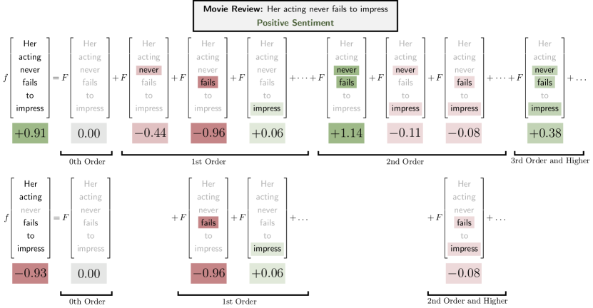
Figure 1: We consider a sentiment analysis problem where the movie review “Her acting never fails to impress” is passed into the BERT language model fine-tuned on the task of sentiment analysis. On the left we present several $1^{st}$, $2^{nd}$ and $3^{rd}$ order Mobius coefficients, with positive valued interactions in green and negative ones in red computed via (2). The Mobius coefficients explain how groups of words influence how BERT perceives the overall sentiment of a sentence. For instance, while never and fails have strongly negative sentiment on their own, when combined, they impose a profound positive sentiment.

Concepts like Shapley value (Lundberg & Lee, 2017) are used to interpret model predictions, assigning importance scores to single inputs (features, data samples, etc.). The Shapley value is the weighted average marginal contribution of a given input, i.e., how much the function changes when the input is included or not. Recent works extend this concept to assigning importance to sets of inputs (Fumagalli et al., 2023; Tsai et al., 2023). What makes all of these representations interpretable is that they represent the function in terms of the marginal effect of inputs (or groups of inputs). The Mobius Transform is a transformation onto this understandable basis that most other explanation techniques use. For instance, a function $f$ with $4$ inputs, $2$ of which are active, can be broken down in terms of its Mobius transform $F$ as illustrated below:

A function is evaluated by summing over all the interactions between all the active inputs, and since the space of all interactions is a basis, the transform $F$ is unique. Other importance metrics can be viewed as projections onto a subset of the Mobius basis. For instance, the Shapley values come from a projection onto the first order basis functions (corresponding to individual marginal effects) under the Shapley kernel error metric.

The complicated functions we learn from deep learning typically do not have boolean inputs, but in order to try to understand them, a common approach is to convert them locally to a function with boolean inputs. Fig. 1 considers a sentiment analysis problem using a version of BERT (Devlin et al., 2019) fine-tuned on the IMDB dataset (Lee, 2023). The objective of the model is to classify the sentiment of the review as positive or negative. Our goal is to understand why the model makes the decision it does. The movie review in Fig. 1 has $n=6$ words. We construct a boolean function $f$, where the inputs determine which of $6$ words are left unmasked before we feed in into BERT. When we mask none of the words (top of Fig 1), BERT correctly determines that the sentiment is positive. Since all the inputs are “active” (not masked), this can be retrieved by summing all Mobius interactions $F$. Generally, we write for $f:\mathbb{Z}_{2}^{n}\rightarrow\mathbb{R}$

$$f(\mathbf{m})=\sum_{\mathbf{k}\leq\mathbf{m}}F(\mathbf{k}),$$ (1)

where $\mathbf{k}\leq\mathbf{m}$ means that $k_{i}\leq m_{i}\;\forall i$. All the inputs being active corresponds to $\mathbf{m}=\bm{1}$, so the inequality condition means we sum over all $2^{6}$ interactions. Examining these interactions can tell us about BERT: it understands double negatives (see the interaction between “never” and “fails”) as well as the positive sentiment of the word “impress”.

Fig. 1 also shows what happens when we mask “never”. Following (1), we exclude interactions involving “never”. Since “never” is involved in many positive interactions, the sentiment is overall negative. This is the power of the Mobius transform: we can see precisely the interactions that cause this shift. This is a significant advantage over first order metrics like the Shapley value. The value of the Mobius transform is apparent, but given its complex structure, is it possible to compute it efficiently? Shown below is the definition of $F$ (this is the “forward” Mobius transform where (1) is the “inverse” transform):

$$F(\mathbf{k})=\sum_{\mathbf{m}\leq\mathbf{k}}(-1)^{\bm{1}^{\textrm{T}}(\mathbf{k}-\mathbf{m})}f(\mathbf{m}).$$ (2)

In general, to compute $F(\mathbf{k})$ for all $\mathbf{k}\in\mathbb{Z}_{2}^{n}$ requires all $2^{n}$ samples from $f$, as well as $n2^{n}$ time using a divide-and-conquer approach similar to that of the Fast Fourier Transform (FFT) algorithm. ChatGPT-3.5 currently supports in the range of $800$ words-per-prompt. Running inference $2^{800}$ times is not even close to possible, and even if you could, $2^{800}$ coefficients is hardly interpretable!

In Fig. 1 we see that many coefficients are small compared to those with the largest magnitude. This is typical. The solution to the computational problem is to just focus on computing the largest Mobius interactions and ignore the small ones. Is this possible in a systematic way? We answer this question in the affirmative. Assuming that for all but $K$ values of $\mathbf{k}$ we have $F(\mathbf{k})=0$ (which $K$ values are significant is unknown), our algorithm enables us to intelligently select points $\bm{$}tosignificantlyreducethenumberofsamplesof$f(m)$thatarerequiredtodetermine$F$to$O(Kn)$with$O(Kn^2)$time.Wealsoexploretheregimewherethenon-zerointeractionsoccurbetweenatmost$t$inputs,with$t ≪n$,showingthatonly$O(Ktlog(n))$samplesarerequiredin$O(Kpoly(n))$time.Wealsohavearobustalgorithmthatallowsforsomenoiseinthesamplingprocess,effectivelyrelaxingtheconstraintthatthe$F(k) = 0$areexactlyzerowhilemaintainingthecomplexity.\par$

1.1 Main Contributions

Our algorithm and proofs are deeply interdisciplinary. We use modern ideas spanning across signal processing, algebra, coding and information theory, and group testing to address this important problem at the forefront of machine learning.

• With $K$ non-zero Mobius coefficients chosen uniformly at random, the Sparse Mobius Transform (SMT) algorithm exactly recovers the transform $F$ in $O(Kn)$ samples and $O(Kn^{2})$ time in the limit as $n\rightarrow\infty$ with $K$ growing at most as $2^{n\delta}$ with $\delta\leq\frac{1}{3}$.

• We develop a formal connection with group testing and present a variant of SMT that works when all non-zero interactions are low order (between only a small number of coordinates). If the maximum order of interaction is $t=\Theta(n^{\alpha})$ where $\alpha<0.409$ then we can compute the Mobius transform in $O(Kt\log(n))$ samples in $O(K\operatorname{poly}(n))$ time with error going to zero as $n\rightarrow\infty$ with growing $K$.

• Leveraging robust group testing, we develop an algorithm that, under certain assumptions, computes the Mobius transform in $O(Kt\log(n))$, with vanishing error in the limit as $n\rightarrow\infty$ with growing $K$.

In addition to our asymptotic performance analysis, we also provide synthetic experiments that verify that our algorithm performs well even in the finite $n$ regime. Furthermore, our results are non-adaptive meaning that sampling can be parallelized. We note that several of our guarantees require that $K$ or $t$ is not too large. For instance, for some results we require $K=O(2^{n\delta})$ with $\delta\leq\frac{1}{3}$.

1.2 Notation

Lowercase boldface $\mathbf{x}$ and uppercase boldface $\mathbf{X}$ denote vectors and matrices respectively. $\mathbf{x}\geq\mathbf{y}$ means that $x_{i}\geq y_{i}\;\forall i$. Multiplication is always standard real field multiplication, but addition between two elements in $\mathbb{Z}_{2}$ should be interpreted as a logical OR $\lor$. We also define subtraction, of $\mathbf{x}-\mathbf{y}$ for $\mathbf{x}\geq\mathbf{y}$ by standard real field subtraction. $\bar{\mathbf{x}}$ corresponds to bit-wise negation for boolean $\mathbf{x}$, and $\mathbf{x}\odot\mathbf{y}$ represents an element-wise multiplication. We say $g_{1}(n)=O(g_{2}(n))$, if there exists some constant $A$ and some $n_{0}$ such that $g_{1}(n)\leq Ag_{2}(n)\;\forall n\geq n_{0}$. We say $g_{1}(n)=\Theta(g_{2}(n))$ if $g_{1}(n)=O(g_{2}(n))$ and there exists some constant $B$ and some $n_{1}$ such that $g_{1}(n)\geq Bg_{2}(n)\;\forall n\geq n_{0}$.

2 Related Works and Applications

This work is inspired by the literature on sparse Fourier transforms, which began with Hassanieh et al. (2012), Stobbe & Krause (2012) and Pawar & Ramchandran (2013). The sparse boolean Fourier (Hadamard) transform (Li et al., 2014; Amrollahi et al., 2019) is most relevant.

Group Testing

This manuscript establishes a strong connection between the interaction identification problem and group testing (Aldridge et al., 2019). Group testing was first described by Dorfman (1943), who noted that when testing soldiers for syphilis, pooling blood samples from many soldiers, and testing the pooled blood samples reduced the total number of tests needed. Zhou et al. (2014) were the first to exploit group testing in a feature selection/importance problem, using a group testing matrix in their algorithm. Jia et al. (2019) also mention group testing in relation to Shapley values.

Mobius Transform

The Mobius transform (Grabisch et al., 2000) is well known in the literature on pseudo-boolean functions (set functions). Wendler et al. (2021) develop a general framework for computing transforms of pseudo-boolean functions. They do not directly consider the Mobius transform as we define it, but their framework can compute a range of $K$ sparse transforms in $O(n^{2}K-nK\log(K))$ adaptive samples and $O(n^{2}K+K^{2}n)$ time. Below, we describe some applications to machine learning.

Explainability

Lundberg & Lee (2017) suggest explaining models by transforming it into a pseudo-boolean function and approximating it using the Shapley value, amounting to only using the first order Mobius coefficients. In Tsai et al. (2023), a higher order version of this idea is introduced, named Faithful Shapley Interaction index (FSI), which uses up to $t$-th order Mobius interactions. In Fumagalli et al. (2023) a new computational approach is devised that generally outperforms other methods for computing the FSI. Other cardinal interaction indices (CII) are also studied. We provide an explanation on the relationship between the Mobius transform, FSI, and standard Shapley value in Appendix A. We also note the many other extensions of Shapley values (Harris et al., 2022; Jullum et al., 2021).

Data Valuation and Auctions

In data valuation (Jia et al., 2019) the goal is to assign an importance score to data, either to determine a fair price (Kang et al., 2023), or to curate a more efficient dataset (Wang & Jia, 2023). A feature of this problem is the high cost of getting a sample, since we need to determine the accuracy of our model when trained on different subsets of data. Ghorbani & Zou (2019); Ghorbani et al. (2020) try to approximate this by looking at the accuracy of partially trained models, though this introduces sampling noise. Banzhaf values have also been proposed as a robust alternative (Wang & Jia, 2023). Combinatorial auctions are another important application area (Leyton-Brown et al., 2000). We discuss auctions more in Section 7.

3 Problem Setup

In general computing (2) requires sampling $f$ for all $2^{n}$ possible input combinations, which is impractical even for modest $n$. For an arbitrary $f$, one cannot do any better. In fact, the same is true of the Shapley value—so why do computational software packages like SHAP (Lundberg & Lee, 2017) exist? It is because interesting $f$ are not arbitrary. If $f$ is a classifier that takes in many features, it is likely some of these features will be complementary (when they appear together, the probability of a class is increased or decreased further) or substitutive (meaning when they occur together, the sum of their effects is diminished). Similarly, it is rather unlikely that there are significant interactions between large numbers of features simultaneously. This idea that only a small fraction of the total $2^{n}$ interactions will be significant is considered in the following assumption:

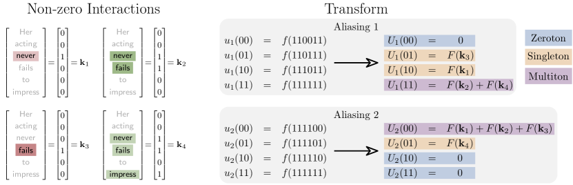
Figure 2: This figure considers a “sparsified” version of the Mobius coefficients depicted in Fig 1, keeping only the largest 4 depicted. Two different sampling choices are shown, as well as the resulting aliasing sets. In the first aliasing set, there is one zeroton, two singletons and one multiton. In the second aliasing set, there is two zerotons, one singleton and one multiton.

Assumption 3.1.

($K$ uniform interactions) $f:\mathbb{Z}_{2}^{n}\mapsto\mathbb{R}$ has a Mobius transform of the following form: $\mathbf{k}_{1},\dotsc,\mathbf{k}_{K}$ are sampled uniformly at random from $\mathbb{Z}_{2}^{n}$, and have $F(\mathbf{k}_{i})\neq 0,\;\forall i\in[K]$, but $F(\mathbf{k})=0$ for all other $\mathbf{k}\in\mathbb{Z}_{2}^{n}$.

We might also expect most of the meaningful interactions to be between a small number of inputs. We characterize this with the following assumption:

Assumption 3.2.

($K$ $t$-degree interactions) $f:\mathbb{Z}_{2}^{n}\mapsto\mathbb{R}$ has a Mobius transform of the following form: $\mathbf{k}_{1},\dotsc,\mathbf{k}_{K}$ are sampled uniformly from $\{\mathbf{k}:\left\lvert\mathbf{k}\right\rvert\leq t,\mathbf{k}\in\mathbb{Z}_{2}^{n}\}$, and have $F(\mathbf{k}_{i})\neq 0,\;\forall i\in[K]$, but $F(\mathbf{k})=0$ other $\mathbf{k}\in\mathbb{Z}_{2}^{n}$.

In practice, we might not expect the non-zero interactions to be exactly zero. We investigate this in Section 5.

4 Algorithm Overview

4.1 Subsampling and Aliasing

In the first part of the algorithm, we perform functional subsampling: We construct $u$, such that for $b<n$

$$u(\bm{\ell})=f(\mathbf{m}_{\bm{\ell}}),\;\;\bm{\ell}\in\mathbb{Z}_{2}^{b},\;\;\mathbf{m}_{\bm{\ell}}\in\mathbb{Z}_{2}^{n},$$ (3)

where we have the freedom to choose $\mathbf{m}_{\bm{\ell}}$. A very important part of the algorithm is understanding that the Mobius transform of $u$, denoted $U$, is related to $F$ via the well-known signal processing phenomenon of aliasing:

$$U(\mathbf{j})=\sum_{\mathbf{k}\in\mathcal{A}(\mathbf{j})}F(\mathbf{k}),$$ (4)

where $\mathcal{A}(\mathbf{j})$ corresponds to an aliasing set determined by $\mathbf{m}_{\bm{\ell}}$. Fig. 2 shows this subsampling procedure on a “sparsified” version of our sentiment analysis example using two different $\mathbf{m}_{\bm{\ell}}$. Our goal is to choose $\mathbf{m}_{\bm{\ell}}$ such that the non-zero values of $F(\mathbf{k})$ are uniformly spread across the aliasing sets, since that makes them easier to recover. If only a single $\mathbf{k}$ with non-zero $F(\mathbf{k})$ ends up in an aliasing set $\mathcal{A}(\mathbf{j})$, we call it a singleton. In Fig. 2, our first subsampling generated two singletons, while our second one generated only one. Maximizing the number of singleton is one of our goals, since we can ultimately use those singetons to construct the Mobius transform. In this work, we have determined two different subsampling procedures that are asymptotically optimal under our two assumptions:

Lemma 4.1.

We choose $\mathbf{m}_{\bm{\ell}}=\overline{\mathbf{H}^{\textrm{T}}\overline{\bm{\ell}}}$, which results in $\mathcal{A}(\mathbf{j})=\{\mathbf{k}:\mathbf{H}\mathbf{k}=\mathbf{j}\}$. $\mathbf{H}$ should be chosen as follows:

1. Under Assumption 3.1, we choose $\mathbf{H}=[\mathbf{I}_{b\times b}\bm{0}_{b,n-b}]$, or any column permutation of this matrix.

2. Under Assumption 3.2 with $t=\Theta(n^{\alpha})$ for $\alpha\leq 0.409$, we choose $\mathbf{H}$ to be $b$ rows of a properly chosen group testing matrix.

If chosen this way, each of the non-zero indices are mapped to the $2^{b}$ sampling sets $\mathcal{A}(\mathbf{j})$ independently and uniformly at random, thus maximizing singletons when $b=\Theta(\log(K))$.

A thorough discussion of this result is provided in Appendix B.2. We also provide a slightly stronger version that extends independence across multiple $\mathbf{H}$, as is required for our overall result. The proof of this lemma touches many areas of mathematics, including the theory of monoids, information theory, and optimal group testing.

4.2 Singleton Detection and Identification

Although singletons are useful, we cannot immediately use them to recover $F(\mathbf{k})$. We first need a way to know that a given $U(\mathbf{j})$ is a singleton. Secondly, we also need a way to identify what value of $\mathbf{k}$ that singleton corresponds to. Section 5 explains how to accomplish both tasks. Below, we discuss the final part of the algorithm with the assumption that we can accomplish both tasks.

4.3 Message Passing to Resolve Collisions

Since we don’t know the non-zero indices beforehand, collisions between multiple non-zero indices ending up in the same aliasing set is inevitable. These are called multitons. One approach to deal with these multitons is to repeat the procedure over again. Thus, we take samples of the form:

$$u_{c}(\bm{\ell})=f(\mathbf{m}_{c,\bm{\ell}}),\iff U_{c}(\mathbf{j})=\sum_{\mathbf{k}\in\mathcal{A}_{c}(\mathbf{j})}F(\mathbf{k}),$$ (5)

$c=1,\dotsc,C$. Each time, we get different aliasing sets $\mathcal{A}_{c}(\mathbf{j})$ and we uncover a different set of singletons, and thus find a different set of $\mathbf{k}$ with non-zero indices $F(\mathbf{k})$. While this approach works, a better approach is to combine this idea with a message passing algorithm to use known non-zero indices and values $(\mathbf{k},F[\mathbf{k}])$ to resolve these multitons and turn them into singletons. The particular type of message passing algorithm we use is called graph peeling. The aliasing structure can be represented as a bipartite graph like in Fig. 3. Each $U_{c}(\mathbf{j})$ is a check node, and each non-zero coefficient $F(\mathbf{k})$ is a variable node. The variable note $F(\mathbf{k})$ is connected to the check node $U_{c}(\mathbf{j})$ if $\mathbf{H}_{c}\mathbf{k}=\mathbf{j}$. Fig. 3 constructs this bipartite graph for the aliasing in Fig. 2. Note that $U_{1}(11)=F(\mathbf{k}_{2})+F(\mathbf{k}_{4})$ is a multiton; however, in the other sub-samping group $U_{2}(01)=F(\mathbf{k}_{4})$ is a singleton. Once we resolve $U_{2}(01)$, we can simply subtract $F(\mathbf{k}_{4})$ from $U_{1}(11)$, allowing us to create a new singleton, and extract $F(\mathbf{k}_{2})$. The remaining values of $F$ both appear as singletons in the first sampling group, so we can resolve all $4$ non-zero interactions $F$ with only $8$ ($7$ unique) samples. Peeling algorithms were first popularized in information and coding theory as a method of decoding fountain codes (Luby, 2002) and have been widely used. They can be analyzed using density evolution theory (Chung et al., 2001), which we use in Appendix B.6 as part of our proof.

5 Singleton Detection and Identification

We have discussed how to subsample efficiently to maximize singletons and how to use message passing to recover as many interactions as possible. Now we discuss (1) how to identify singletons and (2) how to determine the $\mathbf{k}^{*}$ corresponding to the singleton. The following result is key:

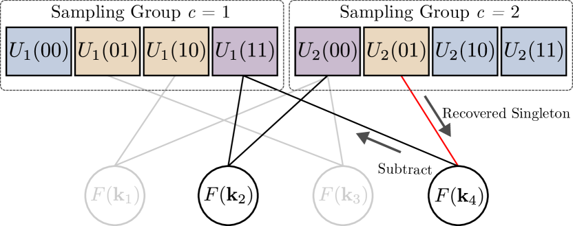
Figure 3: Depiction of our peeling message passing algorithm for the samples in Fig. 2. The singleton in $U_{2}(01)$ is subtracted (peeled) so we can resolve $F(\mathbf{k}_{2})$ from $U_{1}(11)$.

Lemma 5.1.

Consider $\mathbf{H}\in\mathbb{Z}_{2}^{b\times n}$, and $f:\mathbb{Z}_{2}^{n}\mapsto\mathbb{R}$, and some $\mathbf{d}\in\mathbb{Z}_{2}^{n}$. If $U$ is the Mobius transform of $u$, and $F$ is the Mobius transform of $f$ we have:

$$u(\bm{\ell})=f\left(\overline{\mathbf{H}^{\textrm{T}}_{c}\overline{\bm{\ell}}+\mathbf{d}}\right)\iff U(\mathbf{j})=\sum_{\begin{subarray}{c}\mathbf{H}\mathbf{k}=\mathbf{j}\\ \mathbf{k}\leq\mathbf{\overline{d}}\end{subarray}}F(\mathbf{k}).\vspace{-6pt}$$ (6)

The proof is found in Appendix B.4. The form of (6) allows us to reduce the aliasing set in a controlled way. Define $\mathbf{d}_{c,0}\vcentcolon=\bm{0}_{n}$, and $\mathbf{D}_{c}\in\mathbb{Z}_{2}^{P\times n}$ for some $P>0$. The $i^{\text{th}}$ row of $\mathbf{D}_{c}$ is denoted $\mathbf{d}_{c,p}$, $p=1\dotsc,P$. Using these vectors, we construct $C(P+1)$ different subsampled functions $u_{c,p}$:

$$u_{c,p}(\bm{\ell})=f\left(\overline{\mathbf{H}^{\textrm{T}}_{c}\overline{\bm{\ell}}+\mathbf{d}_{c,p}}\right),\;\forall\bm{\ell}\in\mathbb{Z}_{2}^{b}.$$ (7)

Then, we compute the Mobius transform of each $u_{c,p}$ denoted $U_{c,p}$. Let $\mathbf{U}_{c}(\mathbf{j})\vcentcolon=[U_{c,0}(\mathbf{j}),\dotsc,U_{c,P}(\mathbf{j})]^{\textrm{T}}$.

Algorithm 1 Sparse Mobius Transform (SMT)

1:  Input: $\{\mathbf{H}_{c}\}_{c=1}^{C},\;\mathbf{H}_{c}\in\mathbb{Z}_{2}^{b\times n}$, $\{\mathbf{D}_{i}\}_{c=1}^{C}\;\mathbf{D}_{c}\in\mathbb{Z}_{2}^{P\times n}$

2:  $\hat{F}(\mathbf{k})\leftarrow 0\;\forall\mathbf{k}$; $\;\mathcal{K}\leftarrow\emptyset$;

3:  for $c=1$ to $C$ do

4:     for $p=1$ to $P$ do

5:        $u_{c,p}(\bm{\ell})\leftarrow f\left(\overline{\mathbf{H}^{\textrm{T}}_{c}\overline{\bm{\ell}}+\mathbf{d}_{c,p}}\right)\forall\bm{\ell}\in\mathbb{Z}_{2}^{b}$

6:        $U_{c,p}\leftarrow\operatorname{FastMobius}\left(u_{c,p}\right)$

7:     end for

8:  end for

9:  $\mathcal{S}=\left\{(c,\mathbf{j},\mathbf{k},v):\mathrm{Detect}\left(\mathbf{U}_{c}(\mathbf{j})\right)=\mathcal{H}_{S}(\mathbf{k},v)\right\}$

10:  while $\left\lvert\mathcal{S}\right\rvert>0$ do

11:     for $(c,\mathbf{j},\mathbf{k},v)\in\mathcal{S}$ with $\mathbf{k}\in\mathcal{K}$ do

12:        $\hat{F}(\mathbf{k})\leftarrow v$; $\mathcal{K}\leftarrow\mathcal{K}\cup\{\mathbf{k}\}$

13:        for $c=1$ to $C$ do

14:           $\mathbf{U}_{c}(\mathbf{H}_{c}\mathbf{k})\leftarrow\mathbf{U}_{c}(\mathbf{H}_{c}\mathbf{k})-\hat{F}(\mathbf{k})(\bm{1}-\mathbf{D}_{c}\mathbf{k})$

15:        end for

16:     end for

17:     Update $\mathcal{S}$ : Re-run $\mathrm{Detect}\left(\cdot\right)$

18:  end while

19:  Output: $\hat{F}$

The goal of singleton detection is to identify when $\mathbf{U}_{c}[\mathbf{j}]$ reduces to a single term, and for what value $\mathbf{k}$ that term corresponds to. To do so, we define the $\mathrm{Type}\left(\cdot\right)$:

1. $\mathrm{Type}\left(\mathbf{U}_{c}[\mathbf{j}]\right)=\mathcal{H}_{Z}$ denotes a zeroton, for which there does not exist $F[\mathbf{k}]\neq 0$ such that $\mathbf{H}\mathbf{k}=\mathbf{j}$.

2. $\mathrm{Type}\left(\mathbf{U}_{c}[\mathbf{j}]\right)=\mathcal{H}_{S}(\mathbf{k},F[\mathbf{k}])$ denotes a singleton with only one $\mathbf{k}$ with $F[\mathbf{k}]\neq 0$ such that $\mathbf{H}\mathbf{k}=\mathbf{j}$.

3. $\mathrm{Type}\left(\mathbf{U}_{c}[\mathbf{j}]\right)=\mathcal{H}_{M}$ denotes a multiton for which there exists more than one $F[\mathbf{k}]\neq 0$ such that $\mathbf{H}\mathbf{k}=\mathbf{j}$.

In addition, we define the following ratios:

$$y_{c,p}\vcentcolon=1-\frac{U_{c,p}(\mathbf{j})}{U_{c,0}(\mathbf{j})}\;\;p=1,\dotsc,P,$$ (8)

and the corresponding vector $\mathbf{y}_{c}\vcentcolon=[y_{c,1},\dotsc,y_{c,P}]^{\textrm{T}}$. We use the following rule as our best guess for the type:

$$\mathrm{Detect}\left(\mathbf{U}_{c}[\mathbf{j}]\right)\vcentcolon=\begin{cases}\mathcal{H}_{Z},&\mathbf{U}_{c}[\mathbf{j}]=\bm{0}\\ \mathcal{H}_{M},&\mathbf{y}_{c}\notin\{0,1\}^{P}\\ \mathcal{H}_{S}(\mathbf{k},F[\mathbf{k}]),&\mathbf{y}_{c}\in\{0,1\}^{P}\end{cases}.$$ (9)

By considering the definition of $\mathbf{U}_{c}$ it is possible to show that when $\mathrm{Type}\left(\mathbf{U}_{c}[\mathbf{j}]\right)=\mathcal{H}_{S}(\mathbf{k}^{*},F[\mathbf{k}^{*}])$ that

$$\mathbf{y}_{c}=\mathbf{D}_{c}\mathbf{k}^{*}.$$ (10)

Thus, to recover $\mathbf{k}^{*}$, it always suffices to take $\mathbf{D}_{c}=\mathbf{I}$, and thus $P=n$. It also follows immediately that $\mathrm{Detect}\left(\mathbf{U}_{c}[\mathbf{j}]\right)=\mathrm{Type}\left(\mathbf{U}_{c}[\mathbf{j}]\right)$ under this choice. We can’t do better if we don’t have any extra information about $\mathbf{k}^{*}$, but we can if we know $\left\lvert\mathbf{k}^{*}\right\rvert\leq t$ as we show below. Going back to our example in Fig. 2, with $\mathbf{D}_{c}=\mathbf{I}$ we use a total of $8\times 6=48$ samples as opposed to $2^{6}=64$.

Singleton Identification in the Low-Degree Setting

Let’s say we want to determine the singleton from $U_{1}(10)$ in Fig. 2, and we know $\left\lvert\mathbf{k}^{*}\right\rvert\leq 1$. The following $\mathbf{D}_{c}$ suffices:

$$\mathbf{D}_{c}=\begin{pmatrix}1&1&1&1&1&1\\ 1&1&1&1&0&0\\ 1&1&0&0&1&1\\ 1&0&1&0&1&0\end{pmatrix}.$$ (11)

This matrix is essentially doing a binary search. The first row checks if there are any $1$, the next two rows check which third of the vectors the $1$ is in, and the final row resolves any remaining ambiguity. It requires $P=4$, rather than the $P=6$ for $\mathbf{D}_{c}=\mathbf{I}$. If all non-zero $F(\mathbf{k})$ had satisfied $\left\lvert\mathbf{k}\right\rvert\leq 1$, we could use this matrix for our example in Fig. 2. However, we only have $\left\lvert\mathbf{k}\right\rvert\leq 3$, so $\mathbf{D}_{c}$ as in (11) would not suffice. In the case of general $t$ Bay et al. (2022) says that for any scaling of $t$ with $n$, there exists a group testing design $\mathbf{D}_{c}$ with $P=O(t\log(n))$ that can recover $\mathbf{k}^{*}$ in the limit as $n\rightarrow\infty$ with vanishing error in $\operatorname{poly}(n)$ time, also implying $\mathrm{Detect}\left(\mathbf{U}_{c}[\mathbf{j}]\right)$ has vanishing error (see Appendix B.7.2).

Extension to Noisy Setting

It is practically important to relax the assumption that most of the coefficients are exactly zero. To do this, we assume each subsampled Mobius coefficient is corrupted by noise:

$$U_{c,p}(\mathbf{j})=\sum_{\begin{subarray}{c}\mathbf{H}_{c}\mathbf{k}=\mathbf{j}\\ \mathbf{k}\leq\mathbf{\overline{d}}_{p}\end{subarray}}F(\mathbf{k})+Z_{c,p}(\mathbf{j}),\vspace{-6pt}$$ (12)

where $Z_{c,p}(\mathbf{j})\overset{\tiny i.i.d.}{\sim}\mathcal{N}(0,\sigma^{2})$. There are two main changes that must be made compared to the noiseless case. First, we must place an assumption on the magnitude of non-zero coefficients $\left\lvert F(\mathbf{k}_{i})\right\rvert$, such that the signal-to-noise ratio (SNR) remains fixed. Secondly, the matrix $\mathbf{D}_{c}$ must be modified. It now consists of two parts: $\mathbf{D}_{c}=[\mathbf{D}_{c}^{(1)};\mathbf{D}_{c}^{(2)}]$. $\mathbf{D}_{c}^{(2)}\in\mathbb{Z}_{2}^{P_{2}\times n}$ is a standard noise robust Bernoulli group testing matrix. Using the results of (Scarlett & Johnson, 2020), we can show that $P_{2}=O(t\log(n))$ suffices for any fixed SNR. Unlike the noiseless case, the samples from the rows of $\mathbf{D}_{c}^{(2)}$ are not enough to ensure vanishing error of the $\mathrm{Detect}\left(\cdot\right)$ function. For this we construct $\mathbf{D}_{c}^{(1)}$, which is also a Bernoulli group testing matrix, but with a different probability. In Appendix B.7.4 we show that a modified version of $\mathrm{Detect}\left(\cdot\right)$ has vanishing error if $P_{1}=O(t\log(n))$.

6 Theoretical Guarantees

Now that we have discussed all the major components of the algorithm, we present out theoretical guarantees:

Theorem 6.1.

(Recovery with $K$ Uniform Interactions) Let $f$ satisfy Assumption 3.1 for some $K=O(2^{n\delta})$ with $\delta\leq\frac{1}{3}$. For $\{\mathbf{H}_{c}\}_{c=1}^{C}$ chosen as in Lemma B.3 with $b=O(\log(K))$, $C=3$ and $\mathbf{D}_{c}=\mathbf{I}$, Algorithm 1 exactly computes the transform $F$ in $O(Kn)$ samples and $O(Kn^{2})$ time complexity with probability at least $1-O(1/K)$.

Theorem 6.2.

(Noisy Recovery with $K$ $t^{\text{th}}$ Order Interactions) Let $f$ satisfy Assumption 3.2 for some $K$ and $t=\Theta(n^{\alpha})$ for $\alpha\leq 0.409$. For $\{\mathbf{H}_{c}\}_{c=1}^{C}$ chosen as in Lemma B.4 with $b=O(\log(K))$, $C=3$ and $\mathbf{D}_{c}$ chosen as a suitable group testing matrix. Let $U_{c,p}$ be of the form (12) for the noisy case, and let all non-zero $\left\lvert F(\mathbf{k})\right\rvert=\rho$ again for the noisy case only. Algorithm 1 exactly computes the transform $F$ in $O(Kt\log(n))$ samples and $O(K\operatorname{poly}(n))$ time complexity with probability at least $1-O(1/K)$ in both the noisy and noiseless case.

The proof of Theorem 6.1 and 6.2 is provided in Appendix B.5. The argument combines the results on aliasing, singleton detection and peeling. We note that the requirement $\left\lvert F(\mathbf{k})\right\rvert=\rho$ is only due to limitations of group testing theory, and inequality suffices in practice.

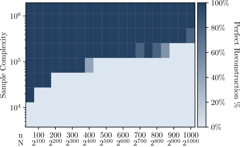
Figure 4: Perfect reconstruction against $n$ and sample complexity under Assumption 3.1. Holding $C=3$, we scale $b$ to increase the sample complexity. We observe that the number of samples required to achieve perfect reconstruction is scaling linearly in $n$ as predicted.

7 Numerical Experiments

7.1 Synthetic Experiments

We now evaluate the performance of SMT on functions generated according to Assumption 3.1 and 3.2. Non-zero coefficients $F(\mathbf{k})$ take values uniformly over $[-1,1]$. We implement SMT as described in Algorithm 1, with group testing decoding via linear programming (Appendix E.2).

Fig. 4 plots the percent of runs where SMT exactly reconstructs $F$ with fixed $K=100$ at different sample complexities and values of $n$. The transition threshold for perfect reconstruction is linear in $n$, as predicted by the theory. Note that we vastly outperform the naive approach: when $n=1000$, we get perfect reconstruction with only $10^{-294}$ percent of total samples!

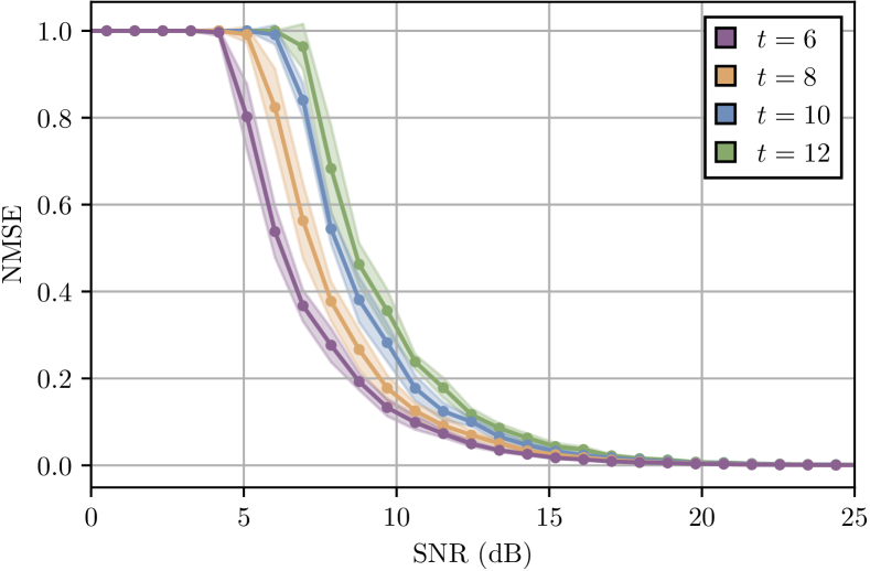
Figure 5: Plot of the noise-robust version of our algorithm. For various values of $t$, we set $n=500$ and $K=500$, using a group testing matrix with $P=1000$. We plot the performance of our algorithm against SNR, measured in terms of the NMSE (13). Error bands represent the standard deviation over $10$ runs.

		Matching	Scheduling
Small Regime	Mobius	$7.4\pm 5.2$	$21.7\pm 11.7$
	Fourier	$214.4\pm 128.3$	$1{,}165.3\pm 1{,}144.1$
Large Regime	Mobius	$12.8\pm 6.1$	$29.5\pm 5.5$
	Samples	$(1.2\pm 2.2)\times 10^{5}$	$(3.6\pm 4.3)\times 10^{5}$
	Time (sec)	$1.69\pm 1.02$	$2.49\pm 0.75$

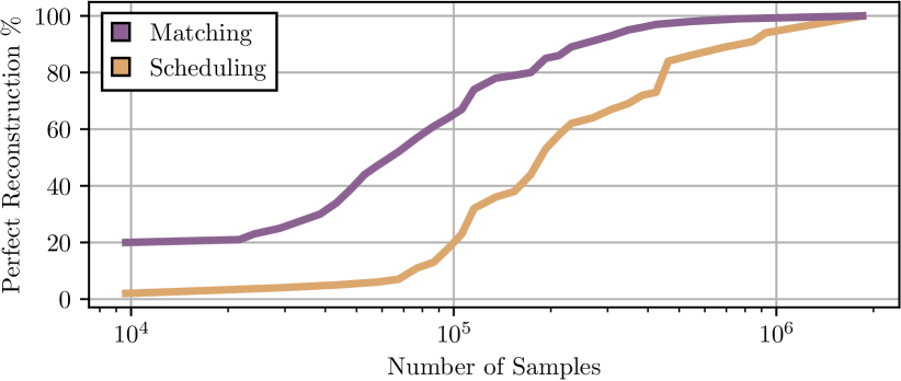
Figure 6: (Left) For both a 20 item and 400 item regimes, we report the mean $\pm$ standard deviation of the sparsity and performance of SMT for the Matching and Scheduling distributions from Leyton-Brown et al. (2000). These distributions model bidder preferences for airport slot allocations and for being allocated time on a shared resource, respectively. (Right) Across 100 realizations of bidder value function for each distribution, we plot the percent of realizations that are perfectly recoverable by SMT for a given number of samples.

Fig. 5 shows SMT under a noisy setting. All other parameters are fixed, with $K=500$, $n=500$, and $P=1000$. We plot the error in terms of

$$\mathrm{NMSE}=\lVert\hat{F}-F\rVert^{2}/\left\lVert F\right\rVert^{2}$$ (13)

versus signal to noise ratio (SNR), where $\hat{F}$ is our estimated Mobius transform. For lower $t$, we see that SMT is more robust. This is because $t=6$ has the most redundant samples, resulting in improved robustness. Increasing $P$ further improves robustness.

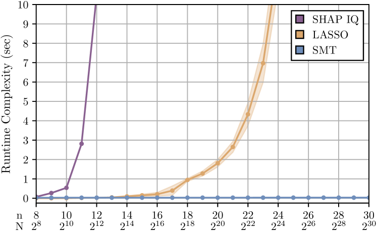
Figure 7: Runtime comparison of SMT, SHAP-IQ (Fumagalli et al., 2023), and $t^{\text{th}}$ order FSI via LASSO (Tsai et al., 2023). All are computing the Mobius transform in the setting where all non-zero interactions are order $t$. SMT easily outperforms both, and scaling as $\log(n)$ while the other methods become intractable. Error bands represent standard deviation over $10$ runs.

Fig. 7 plots the runtime for our algorithm until perfect reconstruction compared to two competing methods. Functions $f$ are sampled such that they each have $K=10$ non-zero Mobius coefficients, and all non-zero interactions have $\left\lvert\mathbf{k}\right\rvert=5$ (restricted to equality rather than inequality due to limitations in the SHAP-IQ code). We compare against SHAP-IQ (Fumagalli et al., 2023) configured to compute the $5^{\text{th}}$ order Faith Shapley Index (FSI), as well as the method of Tsai et al. (2023) which computes $5^{\text{th}}$ order FSI via LASSO. As shown in Appendix A, the $t^{\text{th}}$ order FSI are exactly the $t^{\text{th}}$ order Mobius interactions for our chosen $f$, so all methods compute the same thing. Fig. 7 shows these algorithms scale at least $\operatorname{poly}(n)$ in this setting, while ours scales as $\log(n)$. This figure exemplifies the fact that while these other methods can be useful for small enough $n$, for identifying interactions on the scale of $n\geq 100$, SMT is the only viable option. Additional simulations and discussion can be found in Appendix D.

7.2 Combinatorial Auctions

For large-scale combinatorial auctions, due to the impracticality of collecting complete value functions $f$ over all $2^{n}$ possible allocations over $n$ items, one may seek to elicit bidders’ underlying preferences through a limited number of queries (Conen & Sandholm, 2001). The Mobius transform $F$ identifies the complementary effects between items, such as receiving both a takeoff and landing slot in an airport runway slot allocation auction. We investigate the use of our algorithm to learn and explain bidder value functions for two settings from the Combinatorial Auction Test Suite (Leyton-Brown et al., 2000).

Matching

Many combinatorial auctions concern the allocation of corresponding time chunks across multiple resources, such as an airport slot allocation auction. This distribution models the allocation of runway use for four congested U.S. airports, each with $n/4$ possible time intervals. Bidders (airlines) are interested in securing slots to both takeoff and land along their routes of interest, with sufficient separation to complete the flight.

Scheduling

To manage the use of time on a resource (such as a server or conference room), a combinatorial auction can be used to allocate $n$ time intervals. In this distribution, bidders are interested in receiving a continuous sequence of intervals necessary to complete their task, with their value for a sequence diminishing if not completed by a deadline.

As shown in Weissteiner et al. (2020), many value functions exhibit Fourier sparsity, which can be exploited to learn them with small sample complexity. In Fig. 6, we report the number of Mobius coordinates needed for exact recovery and the number Fourier coordinates necessary to capture 99% of the spectral energy with $n=20$ and $n=400$ items up for auction. While the value functions of bidders can be represented in hundreds or thousands of Fourier coordinates, they can be fully recovered in dozens of Mobius coordinates.

Fig. 6 shows the performance of SMT for recovering value functions under both the matching and scheduling settings when $n=400$. With enough samples, SMT reconstructs the functions perfectly, even though both types of value functions violate Assumptions 3.1 and 3.2 since interactions are heavily correlated. Despite this, our algorithm fully recovers the value function with efficient sample and time complexity, though not as efficiently as our synthetic setting, where our assumptions are satisfied.

8 Conclusion

Identifying interactions between inputs is an important open research question in machine learning, with applications to exaplinability, data valuation, auctions, and many other problems. We approached this problem by studying the Mobius transform, which is a representation over the fundamental interaction basis. We introduced several exciting new tools to the problem of identifying interactions. The use of ideas from sparse signal processing and group testing has allowed SMT to operate in regimes where all other methods fail due to computational burden. Our theoretical results guarantee asymptotic exact reconstruction and are complimented by numerical simulations that show SMT performs well with finite parameters and also under noise.

Future Work

Applying SMT to real world tasks like understanding protein language models (Lin et al., 2022), LLM chatbots (OpenAI, 2023) or diffusion models (Kingma et al., 2021), would be insightful. Working with large and complicated models will likely require further improvements to robustness—both in terms of dealing with noise from small but non-zero interactions, and dealing with potential correlations between interactions. Some interesting ideas in this direction could be using more standards statistical ideas like in Fumagalli et al. (2023), or considering concepts from adaptive group testing. Finally, it would be interesting to see if the techniques used here can improve other algorithms for computing Shapley or Banzhaf values directly.

Impact Statement

Rigorous tools for understanding models can potentially profoundly increase trust in deep learning systems. If we can understand and reason for ourselves why a model is making a decision, we can put greater trust into those decisions. Furthermore, if we understand why a model is doing something that we believe is incorrect, we can better steer it towards doing what we believe is correct. This “steering” of model behavior is sometimes described as alignment, and is a critical task for addressing things like incorrect or misleading information generated by a model, or for address any undesirable biases. In terms of concerns, it is important to not misinterpret or over-interpret the interaction indices that come out of SMT. It could be the case that looking over some selection of interactions doesn’t reveal the full picture, and leads one down an incorrect line of reasoning.

Appendix A Relationship between Mobius Transform and Other Importance Metrics

We being with some notation. We define the Mobius basis function (which are all possible products of inputs) as:

$$b_{\mathbf{k}}(\mathbf{m})\vcentcolon=\prod_{i:k_{i}=1}m_{i}.$$ (14)

Now we define the following sub-spaces of pseudo-boolean function in terms of the linear span of Mobius basis functions:

$$\mathcal{M}_{t}\vcentcolon=\operatorname{span}\{b_{\mathbf{k}}(\mathbf{m}):\left\lvert\mathbf{k}\right\rvert\leq t\}.$$ (15)

Now we define the projection operator $\operatorname{Proj}_{\mu}(f,\mathcal{M}_{t})$, as the projection of the function $f$ onto the $t^{\text{th}}$ order Mobius basis functions with respect to the measure $\mu$. Let $c_{i}$ be the coefficient corresponding to this projection. If $g(\mathbf{m})=\operatorname{Proj}_{\mu}(f,\mathcal{M}_{t})$, we write its decomposition as $g(\mathbf{m})=\sum_{\mathbf{k}\leq t}c(f,\mathcal{M}_{t},\mu,\mathbf{k})b_{\mathbf{k}}(\mathbf{m})$.

Shapley Value

The Shapley values $\operatorname{SV}(i)$ (Shapley, 1952) of the inputs $m_{i},i=1,\dotsc,n$ with respect to the function $f$ are (Hammer & Holzman, 1992):

$$\operatorname{SV}(i)=c(f,\mathcal{M}_{1},\sigma,\mathbf{e}_{i}),$$ (16)

where $\sigma$ is the Shapley kernel. $\operatorname{SV}(i)=F(\mathbf{e}_{i})$ when $f$ is a linear function.

Banzhaf Index

The Banzhaf index $\operatorname{BZ}(i)$ of the inputs $m_{i},i=1,\dotsc,n$ with respect to the function $f$ are (Hammer & Holzman, 1992):

$$\operatorname{BZ}(i)=c(f,\mathcal{M}_{1},\mu,\mathbf{e}_{i}),$$ (17)

where $\mu$ is the uniform measure. $\operatorname{BZ}(i)=F(\mathbf{e}_{i})$ when $f$ is a linear function.

Faith Shapley Interaction Index

The $t^{\text{th}}$ order Faith Shapley interaction index $\operatorname{SV}_{t}(\mathbf{k})$ for $\left\lvert\mathbf{k}\right\rvert\leq t$ (Tsai et al., 2023) is

$$\operatorname{SV}_{t}(\mathbf{k})=c(f,\mathcal{M}_{t},\sigma,\mathbf{k}),$$ (18)

where $\sigma$ is the Shapley kernel. $\operatorname{SV}_{t}(\mathbf{k})=F(\mathbf{k})$ when $f$ is a $t^{\text{th}}$ order function, i.e., $F(\mathbf{k})=0$ when $\left\lvert\mathbf{k}\right\rvert>t$.

Faith Banzhaf Interaction Index

The $t^{\text{th}}$ order Faith Shapley interaction index $\operatorname{BZ}_{t}(\mathbf{k})$ for $\left\lvert\mathbf{k}\right\rvert\leq t$ (Tsai et al., 2023) is

$$\operatorname{BZ}_{t}(\mathbf{k})=c(f,\mathcal{M}_{t},\mu,\mathbf{k}),$$ (19)

where $\mu$ is the uniform measure. $\operatorname{BZ}_{t}(i)=F(\mathbf{k})$ when $f$ is a $t^{\text{th}}$ order function, i.e., $F(\mathbf{k})=0$ when $\left\lvert\mathbf{k}\right\rvert>t$.

Appendix B Missing Proofs

B.1 Boolean Arithmetic

Below we have the addition and multiplication table for arithmetic between $x,y\in\mathbb{Z}_{2}$. We also note that $\mathbb{Z}_{2}$ is typically used to refer to the integer ring modulo $2$. The arithmetic we are describing here is actually that of a monoid. Since the audience for this paper is people interested in machine learning, we continue to use $\mathbb{Z}_{2}$ since it is commonly used to simply refer to the set $\{0,1\}$.

Addition Table
$+$	$x=1$	$x=0$
$y=1$	1	1
$y=0$	1	0

Multiplication Table
$\times$	$x=1$	$x=0$
$y=1$	1	0
$y=0$	0	0

Subtraction Table
$-$	$x=1$	$x=0$
$y=1$	0	1
$y=0$	N/A	0

Table 1: Addition, Multiplication and Subtraction table for boolean arithmetic in this paper. Subtraction is for $y-x$.

B.2 Discussion of Aliasing of the Mobius Transform

When a function has many small or zero Mobius coefficients (interactions), our goal is to subsample (3) in such a way that the aliasing causes the non-zero coefficients to end up in different aliasing sets (4) (as opposed to all of them being aliased together, making them more difficult to reconstruct). Lemma B.1 is a key tool that we will use in this work to design subsampling patterns that result in good aliasing patterns.

Lemma B.1.

Consider $\mathbf{H}\in\mathbb{Z}_{2}^{b\times n}$, $b<n$ and $f:\mathbb{Z}_{2}^{n}\mapsto\mathbb{R}$. Let

$$u(\bm{\ell})=f\left(\overline{\mathbf{H}^{\textrm{T}}\overline{\bm{\ell}}}\right),\;\forall\bm{\ell}\in\mathbb{Z}_{2}^{b}.$$ (20)

If $U$ is the Mobius transform of $u$, and $F$ is the Mobius transform of $f$ we have:

$$U(\mathbf{j})=\sum_{\mathbf{H}\mathbf{k}=\mathbf{j}}F(\mathbf{k}).$$ (21)

This lemma is a powerful tool, allowing us to control the aliasing sets through the matrix $\mathbf{H}$. The proof can be found in Appendix B.3, and is straightforward, given the relationship between $u$ and $f$. Understanding why we choose this relationship, however, is more complicated. Underlying this choice is the algebraic theory of monoids and abstract algebra.

As we have mentioned, our ultimate goal is to design $\mathbf{H}$ to sufficiently “spread out” the non-zero indices among the aliasing sets. Below, we define a simple and useful construction for $\mathbf{H}$.

Definition B.2.

Consider $\{i_{1},\dotsc,i_{b}\}=I\subset[n]$, with $\left\lvert I\right\rvert=b$, and $\mathbf{H}\in\mathbb{Z}_{2}^{b\times n}$. Let $\mathbf{h}_{i}$ correspond to the $i^{\text{th}}$ row of $\mathbf{H}$, given by $\mathbf{h}_{i}=\mathbf{e}_{i_{j}}$, the length $n$ unit vector in coordinate $i_{j}$. Then if we subsample according to (20) we have:

$$U(\mathbf{j})=\sum_{\mathbf{k}\;:\;k_{i}=j_{i}\;\forall i\in I}F(\mathbf{k}).$$ (22)

which happens to result in aliasing sets $\mathcal{A}(\mathbf{j})=\{\mathbf{k}:k_{i}=j_{i}\;\forall i\in I\}$ all of equal size $2^{b}$. The above choice $\mathbf{H}$ actually induces a rather simple sampling procedure when we follow (20). For instance if $I=[b]$, we have:

$$u(\bm{\ell})=f\left([\overline{\bm{\ell}};\bm{1}_{n-b}]\right),$$ (23)

In other words, in this case, we construct samples by freezing $n-b$ of the inputs to $1$ and then varying the remaining $b$ inputs across all the $2^{b}$ possible options. In the case where the non-zero Mobius interactions are chosen uniformly at random, this construction does a good job at spacing them out across the various aliasing sets. The following result formalizes this.

Lemma B.3.

(Uniform interactions) Let $\mathbf{k}_{1},\dotsc,\mathbf{k}_{K}$ be sampled uniformly at random from $\mathbb{Z}_{2}^{n}$, where $F(\mathbf{k}_{i})\neq 0,\;\forall i\in[K]$, but $F(\mathbf{k})=0$ for all other $\mathbf{k}\in\mathbb{Z}_{2}^{n}$. Construct disjoint sets $I_{c}\subset[n]$ for $c=1,\dotsc,C$, and the corresponding matrix $\mathbf{H}_{c}$ according to Definition B.2. Let $\mathcal{A}_{c}(\mathbf{j})$ correspond to the aliasing sets after sampling with respect to matrix $\mathbf{H}_{c}$. Now define:

$$\mathbf{j}\text{ such that }\mathbf{k}_{i}\in\mathcal{A}_{c}(\mathbf{j})\vcentcolon=\mathbf{j}_{i}^{c}.$$ (24)

Then if $b=O(\log(K))$, $K=O(2^{n/C})$, in the limit as $n\rightarrow\infty$ with $C=O(1)$, $\mathbf{j}_{i}^{c}$ are mutually independent and uniformly distributed over $\mathbb{Z}_{2}^{b}$.

The proof is given in Appendix B.6.1, and follows directly from the form of the aliasing sets $\mathcal{A}_{c}(\mathbf{j})$. Corollary B.3 means that using $\mathbf{H}$ as constructed in Definition B.2 ensures that we all $\mathbf{k}$ with $F(\mathbf{k})\neq 0$ are uniformly distributed over the aliasing sets, which maximizes the number of singletons. This result, however, hinges on the fact that the non-zero coefficients are uniformly distributed. We are also interested in the case where the non-zero coefficients are all low-degree. In order to induce a uniform distribution in this case, we need to exploit a group testing matrix.

Lemma B.4.

(Low-degree interactions) Let $\mathbf{k}_{1},\dotsc,\mathbf{k}_{K}$ be sampled uniformly at random from $\{\mathbf{k}:\left\lvert\mathbf{k}\right\rvert\leq t,\mathbf{k}\in\mathbb{Z}_{2}^{n}\}$, where $F(\mathbf{k}_{i})\neq 0,\;\forall i\in[K]$, but $F(\mathbf{k})=0$ for all other $\mathbf{k}\in\mathbb{Z}_{2}^{n}$. By constructing $C$ matrices $\mathbf{H}_{c},c=1,\dotsc,C$ from rows of a near constant column weight group testing matrix, and sampling as in (20), if $t=\Theta(n^{\alpha})$ for $\alpha<0.409$, and $b=O(\log(K))$, $K=O(n^{t})$, in the limit as $n\rightarrow\infty$, $\mathbf{j}_{i}^{c}$ as defined in (24) are mutually independent and uniformly distributed over $\mathbb{Z}_{2}^{b}$.

The proof is given in Appendix B.6.2. It relies on an information theoretic argument, exploiting a result from optimal group testing (Coja-Oghlan et al., 2020).

B.3 Proof of Lemma B.1

Proof.

Taking the Mobius transform of $u$ gives us:

$$U(\mathbf{k}) = \sum_{\bm{\ell}\leq\mathbf{k}}(-1)^{\mathds{1}^{T}(\mathbf{k}-\bm{\ell})}u(\bm{\ell})$$

$$= \sum_{\bm{\ell}\leq\mathbf{k}}(-1)^{\mathds{1}^{T}(\mathbf{k}-\bm{\ell})}f\left(\bigodot_{i:\ell_{i}=0}\mathbf{\overline{h}}_{i}\right)$$

$$= \sum_{\bm{\ell}\leq\mathbf{k}}(-1)^{\mathds{1}^{T}(\mathbf{k}-\bm{\ell})}\sum_{\mathbf{r}\leq\bigodot_{i:\ell_{i}=0}\mathbf{\overline{h}}_{i}}F(\mathbf{r})$$

$$= \sum_{\bm{\ell}\in\mathbb{Z}_{2}^{b}}(-1)^{\mathds{1}^{T}(\mathbf{k}-\bm{\ell})}\mathds{1}\{\bm{\ell}\leq\mathbf{k}\}\sum_{\mathbf{r}\in\mathbb{Z}_{2}^{n}}F(\mathbf{r})\mathds{1}\left\{\mathbf{r}\leq\bigodot_{i:\ell_{i}=0}\mathbf{\overline{h}}_{i}\right\}$$

$$= \sum_{\mathbf{r}\in\mathbb{Z}_{2}^{n}}F(\mathbf{r})\left(\sum_{\bm{\ell}\in\mathbb{Z}_{2}^{b}}(-1)^{\mathds{1}^{T}(\mathbf{k}-\bm{\ell})}\mathds{1}\{\bm{\ell}\leq\mathbf{k}\}\mathds{1}\left\{\mathbf{r}\leq\bigodot_{i:\ell_{i}=0}\mathbf{\overline{h}}_{i}\right\}\right)$$

$$= \sum_{\mathbf{r}\in\mathbb{Z}_{2}^{n}}F(\mathbf{r})I(\mathbf{r})$$

Now let’s just focus on the term in the parenthesis for now, which we have called $I(\mathbf{r})$.

Case 1: $\mathbf{H}\mathbf{r}=\mathbf{k}$

$$I(\mathbf{r}) = \sum_{\bm{\ell}\leq\mathbf{k}}(-1)^{\mathds{1}^{T}(\mathbf{k}-\bm{\ell})}\mathds{1}\left\{\mathbf{r}\leq\bigodot_{i:\ell_{i}=0}\mathbf{\overline{h}}_{i}\right\}$$ (25)

First note that under this condition, $\bm{\ell}=\mathbf{k}\implies\mathbf{r}\leq\bigodot_{i:\ell_{i}=0}\mathbf{\overline{h}}_{i}$. To see this, note that $k_{j}=0\implies\mathbf{r}\leq\mathbf{\overline{h}}_{j}$. Since this holds for all $j$ such that $k_{j}=0$, we have the previously mentioned implication.

Conversely, if $\ell_{j}<k_{j}$ (this means $\ell_{j}=0$ AND $k_{j}=1$) for some $j$, then $\mathbf{r}$ and $\mathbf{h}_{j}$ must overlap. Thus,

$$\mathds{1}\left\{\mathbf{r}\leq\mathbf{\overline{h}}_{j}\right\}=0\implies\mathds{1}\left\{\mathbf{r}\leq\bigodot_{i:\ell_{i}=0}\mathbf{\overline{h}}_{i}\right\}=0$$

We can split $I(\mathbf{r})$ into two parts, the part where $\bm{\ell}=\mathbf{k}$ and the part where $\bm{\ell}<\mathbf{k}$:

$$I(\mathbf{r}) = \mathds{1}\left\{\mathbf{r}\leq\bigodot_{i:\mathbf{k}_{i}=0}\mathbf{\overline{h}}_{i}\right\}+\sum_{\bm{\ell}<\mathbf{k}}(-1)^{\mathds{1}^{T}(\mathbf{k}-\bm{\ell})}\mathds{1}\left\{\mathbf{r}\leq\bigodot_{i:\ell_{i}=0}\mathbf{\overline{h}}_{i}\right\}\quad(\mathbf{H}\mathbf{r}=\mathbf{k})$$ (26)

$$= 1+\sum_{\bm{\ell}<\mathbf{k}}0$$ (27)

$$= 1$$ (28)

Case 2: $\mathbf{H}\mathbf{r}\neq\mathbf{k}$

Let $\mathbf{H}\mathbf{r}=\mathbf{k}^{\prime}\neq\mathbf{k}$. This case itself will be broken into two parts. First let’s say there is some $j$ such that $k_{j}=0$ and $k_{j}^{\prime}=1$. Since $k^{\prime}_{j}=1$ we know that $\mathds{1}\left\{\mathbf{r}\leq\mathbf{\overline{h}}_{j}\right\}=0$. Furthermore, since $\forall\bm{\ell}\in\{\bm{\ell}:\bm{\ell}\leq\mathbf{k}\}$ we have $\ell_{j}=0$. Then by a similar argument to our previous one, we have $\mathds{1}\left\{\mathbf{r}\leq\bigodot_{i:\ell_{i}=0}\mathbf{\overline{h}}_{i}\right\}=0\;\forall\bm{\ell}\leq\mathbf{k}$. It follows immediately that $I(\mathbf{r})=0$ in this case.

Finally, we have the case where $\mathbf{k}^{\prime}<\mathbf{k}$. First, if there is a coordinate $j$ such that $0=\ell_{j}<k^{\prime}_{j}=1$, we know that $\mathds{1}\left\{\mathbf{r}\leq\mathbf{\overline{h}}_{j}\right\}=0$ so we have $\mathds{1}\left\{\mathbf{r}\leq\bigodot_{i:\ell_{i}=0}\mathbf{\overline{h}}_{i}\right\}=0\;\forall\bm{\ell}$ s.t. $\exists j,\ell_{j}<k^{\prime}_{j}$. The only $\bm{\ell}$ that remain are those such that $\mathbf{k}^{\prime}\leq\bm{\ell}\leq\mathbf{k}$. It is easy to see that this is a sufficient condition for $\mathds{1}\left\{\mathbf{r}\leq\bigodot_{i:\ell_{i}=0}\mathbf{\overline{h}}_{i}\right\}=1$.

$$I(\mathbf{r}) = \sum_{\bm{\ell}\leq\mathbf{k}}(-1)^{\mathds{1}^{T}(\mathbf{k}-\bm{\ell})}\mathds{1}\left\{\mathbf{r}\leq\bigodot_{i:\ell_{i}=0}\mathbf{\overline{h}}_{i}\right\}$$ (29)

$$= \sum_{\mathbf{k}^{\prime}\leq\bm{\ell}\leq\mathbf{k}}(-1)^{\mathds{1}^{T}(\mathbf{k}-\bm{\ell})}$$ (30)

$$= 0$$ (31)

Where the final sum is zero because exactly half of the $\bm{\ell}$ have even and odd parity respectively.

Thus, the subsampling pattern becomes:

$$U(\mathbf{k})=\sum_{\mathbf{H}\mathbf{r}=\mathbf{k}}F(\mathbf{r}).$$

∎

B.4 Proof of Section 5

$$U(\mathbf{k}) = \sum_{\bm{\ell}\leq\mathbf{k}}(-1)^{\mathds{1}^{T}(\mathbf{k}-\bm{\ell})}u(\bm{\ell})$$

$$= \sum_{\bm{\ell}\leq\mathbf{k}}(-1)^{\mathds{1}^{T}(\mathbf{k}-\bm{\ell})}f\left(\left(\bigodot_{i:\ell_{i}=0}\mathbf{\overline{h}}_{i}\right)\odot\mathbf{\overline{d}}\right)$$

$$= \sum_{\bm{\ell}\leq\mathbf{k}}(-1)^{\mathds{1}^{T}(\mathbf{k}-\bm{\ell})}\sum_{\mathbf{r}\leq\bigodot_{i:\ell_{i}=0}\mathbf{\overline{h}}_{i}}F(\mathbf{r})\mathds{1}\left\{\mathbf{r}\leq\mathbf{\overline{d}}\right\}$$

$$= \sum_{\bm{\ell}\in\mathbb{Z}_{2}^{b}}(-1)^{\mathds{1}^{T}(\mathbf{k}-\bm{\ell})}\mathds{1}\{\bm{\ell}\leq\mathbf{k}\}\sum_{\mathbf{r}\in\mathbb{Z}_{2}^{n}}F(\mathbf{r})\mathds{1}\left\{\mathbf{r}\leq\bigodot_{i:\ell_{i}=0}\mathbf{\overline{h}}_{i}\right\}\mathds{1}\left\{\mathbf{r}\leq\mathbf{\overline{d}}\right\}$$

$$= \sum_{\mathbf{r}\in\mathbb{Z}_{2}^{n}}F(\mathbf{r})\mathds{1}\left\{\mathbf{r}\leq\mathbf{\overline{d}}\right\}\left(\sum_{\bm{\ell}\in\mathbb{Z}_{2}^{b}}(-1)^{\mathds{1}^{T}(\mathbf{k}-\bm{\ell})}\mathds{1}\{\bm{\ell}\leq\mathbf{k}\}\mathds{1}\left\{\mathbf{r}\leq\bigodot_{i:\ell_{i}=0}\mathbf{\overline{h}}_{i}\right\}\right)$$

$$= \sum_{\mathbf{r}\in\mathbb{Z}_{2}^{n}}F(\mathbf{r})\mathds{1}\left\{\mathbf{r}\leq\mathbf{\overline{d}}\right\}I(\mathbf{r})$$

$$= \sum_{\begin{subarray}{c}\mathbf{H}\mathbf{r}=\mathbf{k}\\ \mathbf{r}\leq\mathbf{\overline{d}}\end{subarray}}F(\mathbf{r})$$

B.5 Proof of Main Theorems

See 6.1

See 6.2

Proof.

The first step for proving both Theorem 6.1 and Theorem 6.2 is to show that Algorithm 1 can successfully recover all Mobius coefficients with probability $1-O(1/K)$ under the assumption that we have access to a $\mathrm{Detect}\left(\mathbf{U}_{c}(\mathbf{j})\right)$ function that can output the type $\mathrm{Type}\left(\mathbf{U}_{c}(\mathbf{j})\right)$ for any aliasing set $\mathbf{U}_{c}(\mathbf{j})$. Under this assumption, we use density evolution proof techniques to obtain Theorem B.5 and conclude both theorems.

Then, to remove this assumption, we need to show that we can process each aliasing set $\mathbf{U}_{c}(\mathbf{j})$correctly, meaning that each bin is correctly identified as a zeroton, singleton, or multiton. Define $\mathcal{E}$ as the error event where the detector makes a mistake in $O(K)$ peeling iterations. If the error probability satisfies $\mathrm{Pr}(\mathcal{E})\leq O(1/K)$, the probability of failure of the algorithm satisfies

$$\mathbb{P}_{F} =\mathrm{Pr}\left(\widehat{F}\neq F|\mathcal{E}^{\mathrm{c}}\right)\mathrm{Pr}(\mathcal{E}^{\mathrm{c}})+\mathrm{Pr}\left(\widehat{F}\neq F|\mathcal{E}\right)\mathrm{Pr}(\mathcal{E})$$

$$\leq\mathrm{Pr}\left(\widehat{F}\neq F|\mathcal{E}^{\mathrm{c}}\right)+\mathrm{Pr}(\mathcal{E})$$

$$=O(1/K).$$

In the following, we describe how we achieve $\mathrm{Pr}(\mathcal{E})\leq O(1/K)$ under different scenarios.

In the case of uniformly distributed interactions without noise, singleton identification and detection can be performed without error as described in Section B.7.1. In the case of interactions with low-degree and without noise, singleton identification and detection can be performed with vanishing error as described in Section B.7.2. Lastly, we can perform noisy singleton identification and detection with vanishing error for low-degree interactions as described in Section B.7.2.

∎

B.6 Density Evolution Proofs

The density evolution proof is generally separated into two parts.

• We show that with high probability, nearly all of the variable nodes will be resolved.

• We show that with high probability, the graph is a good expander, which ensures that if only a small number are unresolved, the remaining variable nodes will be resolved.

Whether the decoding succeeds or fails depends entirely on the graph (or rather distribution over graphs) that is induced by the algorithm. The graph ensemble is parameterized as $\mathcal{G}\left(\mathcal{D},\left\{\mathbf{M}_{c}\right\}_{c\in[C]}\right)$. $\mathcal{D}$ is the support distribution. The set of non-zero Mobius coefficients $\left\{\mathbf{r}:\mathcal{M}[f](\mathbf{r})\neq 0\right\}\sim\mathcal{D}$ is drawn from this distribution. In (Li et al., 2014), using the arguments above it is shown that if the following conditions hold, the peeling message passing successfully resolves all variable nodes:

1. In the limit as $n\rightarrow\infty$ asymptotic check-node degree distribution from an edge perspective converges to that of independent an identically distributed Poisson distribution (shifted by 1).

2. The variable nodes have a constant degree $C\geq 3$ (This is needed for the expander property).

3. The number of check nodes $b$ in each of the $C$ sampling group is such that $2^{b}=O(K)$.

Theorem B.5 (Li et al. (2014)).

If the above three conditions hold, the peeling decoder recovers all Mobius coefficients with probability $1-O(1/K)$.

In the following section, we show that for suitable choice of sampling matrix, these conditions are satisfied, both in the case of uniformly distributed and low degree Mobius coefficients.

B.6.1 Uniform Distribution

In order to satisfy the conditions for the case of a uniform distribution of we use the matrix in Corollary B.3. We select $C=3$ different $I_{1},I_{2},I_{3}$ such that $I_{i}\cap I_{j}=\emptyset\;\;\forall i\neq j\in\{1,2,3\}$. Note that this satisfies condition (2) above. Furthermore, we let $k$ scale as $O(2^{n\delta})$. In order to satisfy condition (3), we must have $\delta<\frac{1}{3}$, since each $I_{i}$ can consist of at most $\frac{1}{3}$ of all the coordinates.

We now introduce some notation. Let $\mathbf{g}_{j}(\cdot)$ represent the hash function, that maps a frequency $\mathbf{r}$ to a check node index $\mathbf{k}$ in each subsampling group $j=1,\dotsc,C$, i.e., $\mathbf{g}_{j}(\mathbf{r})=\mathbf{H}_{j}\mathbf{r}$. Per our assumption, we have $K$ non-zero variable notes $\mathbf{r}^{(1)},\dotsc,\mathbf{r}^{(K)}$ chosen uniformly at random. Technically, we are sampling without replacement, however, since $\frac{K}{2^{n}}\rightarrow 0$, the probability of selecting a previously selected $\mathbf{r}^{(i)}$ vanishes. Going forward in this subsection, we will assume that each $\mathbf{r}_{i}$ is sampled with replacement for a more brief solution. A more careful analysis that deals with sampling with replacement before taking limits yields an identical result.

First, let’s consider the marginal distribution of $\mathbf{g}_{j}(\mathbf{r}^{(i)})$ for some arbitrary $j\in[C]$ and $i\in[K]$. Assuming sampling with replacement, we have:

$$\Pr\left(\mathbf{g}_{j}(\mathbf{r}^{(i)})=\mathbf{k}\right)=\Pr\left(\mathbf{r}^{(i)}_{I_{j}}=\mathbf{k}\right)=\prod_{m\in I_{j}}\Pr\left(r^{(i)}_{m}=k_{m}\right)=\frac{1}{2^{b}}.$$ (32)

Thus, we have established that the our approach induces a uniform marginal distribution over the $2^{b}$ check nodes. Next, we consider the independence of our bins. By assuming sampling with replacement, we can immediately factor our probability mass function.

$$\Pr\left(\bigcap_{i,j}\mathbf{g}_{j}(\mathbf{r}^{(i)})=\mathbf{k}^{(i,j)}\right)=\prod_{i}\Pr\left(\bigcap_{j}\mathbf{g}_{j}(\mathbf{r}^{(i)})=\mathbf{k}^{(i,j)}\right)$$ (33)

Furthermore, since we carefully chose the $I_{i}$ such that they are pairwise disjoint, we have

$$\Pr\left(\bigcap_{j}\mathbf{g}_{j}(\mathbf{r}^{(i)})=\mathbf{k}^{(i,j)}\right)=\Pr\left(\bigcap_{j}\mathbf{r}^{(i)}_{I_{j}}=\mathbf{k}^{(i,j)}\right)=\prod_{j}\Pr\left(\mathbf{r}^{(i)}_{I_{j}}=\mathbf{k}^{(i,j)}\right)=\prod_{j}\Pr\left(\mathbf{g}_{j}(\mathbf{r}^{(i)})=\mathbf{k}^{(i,j)}\right),$$ (34)

establishing independence. Let’s define an inverse load factor $\eta=\frac{2^{b}}{K}$. From a edge perspective, sampling with replacement with independent uniformly distributed gives us:

$$\rho_{j}=j\eta\binom{K}{j}\left(\frac{1}{2^{b}}\right)^{j}\left(1-\frac{1}{2^{b}}\right)^{k-j},$$ (35)

For fixed $\eta$, asymptotically as $K\rightarrow\infty$ this converges to:

$$\rho_{j}\rightarrow\frac{(1/\eta)^{j-1}e^{-1/\eta}}{{(j-1)!}}.$$ (36)

B.6.2 Low-Degree Distribution

For this proof, we take an entirely different approach to the uniform case. We instead exploit the results of Theorem E.1, which is about asymptotically exactly optimal group testing, and then make an information-theoretic argument. Let $\mathbf{X}^{n}$ be a group testing matrix (constructed either by an i.i.d. Bernoulli design or a constant column weight design using the parameters required for the given $n$). We don’t explicitly write the dependence of $\mathbf{X}^{n}$ on $t$, since by invoking Theorem E.1, we assume some implicit relationship where $t=\Theta(n^{\theta})$ for $\theta$ satisfying the theorem conditions. Now consider some $\mathbf{r}_{n}$ chosen uniformly at random from the $\binom{n}{t}$ weight $t$ binary vectors. Note that in this work we actually use what is known as the “i.i.d prior” as opposed to the “combinatorial prior” that we have just defined. As noted in (Aldridge et al., 2019), these are actually equivalent, so we can arbitrarily choose to work with one, and the result holds for the other as well. We define:

$$\mathbf{Y}^{n}=\mathbf{X}^{n}\mathbf{r}^{n}.$$ (37)

Furthermore, we define the decoding function $\operatorname{Dec}_{n}(\cdot)$, which represents the deterministic procedure that successfully recovers $\mathbf{r}$ with vanishing error probability. We have the following bounds on the entropy of $\mathbf{Y}_{n}$:

$$H(\mathbf{Y}^{n}) = H(Y^{n}_{1})+H(Y^{n}_{2}\mid Y^{n}_{1})+\dots+H(Y^{n}_{T}\mid Y^{n}_{1},\dotsc,Y^{n}_{T-1})$$ (38)

$$\leq T,$$ (39)

where we have used the fact that binary random variables have a maximum entropy of $1$. Furthermore, by the properties of entropy we also have $H(\mathbf{Y}^{n})\geq H(\operatorname{Dec}(\mathbf{Y}^{n},\mathbf{X}^{n})\mid\mathbf{X}^{n})$. Dividing through by $T$, we have:

$$\frac{H(\operatorname{Dec}(\mathbf{Y}^{n},\mathbf{X}^{n})\mid\mathbf{X}^{n}))}{T}\leq\frac{H(\mathbf{Y}^{n})}{T}\leq 1.$$ (40)

Let $\operatorname{Dec}_{n}(\mathbf{Y}^{n},\mathbf{X}^{n}))=\mathbf{r}^{n}+\operatorname{err}_{n}(\mathbf{Y}^{n},\mathbf{X}^{n})$. It is known (see (Aldridge et al., 2019)) that $\Pr(\operatorname{err}_{n}(\mathbf{Y}^{n},\mathbf{X}^{n})\neq 0)=O(\operatorname{poly}(T)e^{-T})$. Thus, we can bound the left-hand side as:

$$\frac{H(\operatorname{Dec}(\mathbf{Y}^{n},\mathbf{X}^{n})\mid\mathbf{X}^{n})}{T} = \frac{H(\mathbf{r}^{n}+\operatorname{err}_{n}(\mathbf{Y}^{n},\mathbf{X}^{n})\mid\mathbf{X}^{n})}{T}$$ (41)

$$\geq \frac{H(\mathbf{r}^{n})-H(\operatorname{err}_{n}(\mathbf{Y}^{n},\mathbf{X}^{n})\mid\mathbf{X}^{n})}{T}$$ (42)

$$\geq \frac{H(\mathbf{r}^{n})-H(\operatorname{err}_{n}(\mathbf{Y}^{n},\mathbf{X}^{n}))}{T},$$ (43)

Where in (42) we have used the bound $H(A+B)\geq H(A)-H(B)$ and the fact that $\mathbf{X}^{n}$ and $\mathbf{r}^{n}$ are independent, and in (43) we have used the fact that conditioning only decreases entropy. By the continuity of entropy and Theorem E.1, we have that:

$$\lim_{n\rightarrow\infty}\frac{H(\mathbf{r}^{n})-H(\operatorname{err}_{n}(\mathbf{Y}^{n},\mathbf{X}^{n}))}{T}=\lim_{n\rightarrow\infty}\frac{\log\binom{n}{t}}{T}-\lim_{n\rightarrow\infty}\frac{H(\operatorname{err}_{n}(\mathbf{Y}^{n},\mathbf{X}^{n}))}{T}=1-0=1.$$ (44)

This establishes that:

$$\lim_{n\rightarrow\infty}\frac{1}{T(n)}\sum_{i=1}^{T(n)}H\left(Y^{n}_{i}\mid\mathbf{Y}^{n}_{1:(i-1)}\right)=1.$$ (45)

Unfortunately, this does not immediately imply that all of the summands have a limit of $1$, however, it does mean that the fraction of total summands that are less than one goes to zero (it grows as $o(T(n))$). Let $G\subset\mathbb{N}$ correspond to the set containing all the indicies $i$ of the summands that are equal to $1$. By using the fact that conditioning only reduces entropy, we have

$$\lim_{n\rightarrow\infty}H\left(Y^{n}_{i}\mid\mathbf{Y}^{n}_{S_{i}}\right)=1,\;\;S_{i}=\{j<i,j\in G\},$$ (46)

Now we define the countable sequence of random variables:

$$\bar{Y_{i}}=\lim_{n\rightarrow\infty}Y^{n}_{i},\;i\in\mathbb{N}.$$ (47)

By continuity of entropy, and the above limit and definition, we have:

$$H\left(\bar{Y_{i}}\mid\bar{\mathbf{Y}}_{S_{i}}\right)=1,$$ (48)

Noting that conditioning only decreases entropy, we immediately have that $\bar{Y}_{i}\sim\operatorname{Bern}(\frac{1}{2})$. Now consider some arbitrary finite set $S^{*}\subset G$. We will now prove that $\{\bar{Y}_{i},i\in S^{*}\}$ is mutually independent.

Proof.

Let $i_{1}<i_{2}<\dotsc<i_{\left\lvert S^{*}\right\rvert}$ be an ordered indexing of the elements of $S^{*}$. Furthermore, let $Q_{j}=\left\{i_{q}\mid 1\leq q\leq j\right\}$. Assume the set $\{\bar{Y}_{i},i\in Q_{j}\}$ is mutually independent, and use the notation $\mathbf{Y}_{Q_{j}}$ to represent a vector containing all of these entries. We have:

$$H(Y_{i_{j+1}},\mathbf{Y}_{Q_{j}})=H(\mathbf{Y}_{Q_{j}})+H(Y_{i_{j+1}}\mid\mathbf{Y}_{Q_{j}}).$$ (49)

However, by using the fact that conditioning only decreases entropy we have:

$$1=H(Y_{i_{j+1}}\mid\mathbf{Y}_{S_{j+1}})\leq H(Y_{i_{j+1}}\mid\mathbf{Y}_{Q_{j}})\leq H(Y_{i_{j+1}})\leq 1,$$ (50)

thus,

$$H(Y_{i_{j+1}}\mid\mathbf{Y}_{Q_{j}})=H(Y_{i_{j+1}})=1.$$ (51)

This leads to the following chain of implications:

$$H(Y_{i_{j+1}},\mathbf{Y}_{Q_{j}})=H(\mathbf{Y}_{Q_{j}})+H(Y_{i_{j+1}})\iff Y_{i_{j+1}}\perp\!\!\!\perp\mathbf{Y}_{Q_{j}}.$$ (52)

From this, and the initial inductive assumption, we can conclude that $\{\bar{Y}_{i},i\in Q_{j+1}\}$ is mutually independent. The base case of $j=1$ follows from the fact that a set containing just one single random variable is mutually independent. Since $Q_{\left\lvert S^{*}\right\rvert}=S^{*}$ the proof is complete. ∎

Now let $L(n)=\left\lvert G\cap[n]\right\rvert$ we know $L=\Theta(T(n))$, which follows from the stronger result that $\lim_{n\rightarrow\infty}\frac{L(n)}{T(n)}=1$. Take $b\leq\frac{L(n)}{C}$ By leveraging the above results, we can select our subsampling matrices $\{\mathbf{H}_{i}\}_{i=1}^{C}$ from suitable rows of $\mathbf{X}_{n}$. Let $S^{(n)}_{1},\dotsc,S^{(n)}_{C}\subset G\cap[n]$, $\left\lvert S^{(n)}_{i}\right\rvert=b$ and $S^{(n)}_{i}\cap S^{(n)}_{j}=\emptyset$. Then take

$$\mathbf{H}_{i}(n)=\mathbf{X}^{n}_{S_{i},:}.$$ (53)

Due to the independence result proved above, the asymptotic degree distribution is:

$$\rho_{j}\rightarrow\frac{(1/\eta)^{j-1}e^{-1/\eta}}{{(j-1)!}}.$$ (54)

B.7 Singleton Detection and Identification

B.7.1 Uniform Interactions Singleton Identification and Detection without Noise

Consider a multiton where $\mathbf{U}_{c}(\mathbf{j})=F(\mathbf{k}_{1})+F(\mathbf{k}_{2})$ for $\mathbf{k}_{1}\neq\mathbf{k}_{2}$. Since any two binary vectors must differ in at least one location, there must exist some $p$ such that

$$y_{c,p}=\frac{F_{\mathbf{k}_{1}}}{F_{\mathbf{k}_{1}}+F_{\mathbf{k}_{2}}}\notin\{0,1\},$$ (55)

or

$$y_{c,p}=\frac{F_{\mathbf{k}_{2}}}{F_{\mathbf{k}_{1}}+F_{\mathbf{k}_{2}}}\notin\{0,1\}.$$ (56)

Furthermore, since (10) always exactly recovers $\mathbf{k}^{*}$, we have that $\mathrm{Detect}\left(\mathbf{U}_{c}(\mathbf{j})\right)=\mathrm{Type}\left(\mathbf{U}_{c}(\mathbf{j})\right)$.

B.7.2 Low-Degree Singleton Identification and Detection without Noise

In this case, we can simply rely on the result of Bay et al. (2022). Since $\Pr(\hat{\mathbf{k}}\neq\mathbf{k}^{*})\rightarrow 0$, we correctly recover $\mathbf{k}^{*}$ in the limit, Furthermore, if $\mathbf{U}_{c}(\mathbf{j})=F(\mathbf{k}_{1})+F(\mathbf{k}_{2})$, we also must have $\Pr(\mathbf{D}_{c}\mathbf{k}_{1}\neq\mathbf{D}_{c}\mathbf{k}_{2})\rightarrow 1$. Thus, by the same argument as above, we must also have $\mathbf{y}_{c}\notin\{0,1\}^{n}$ in the limit, implying that $\mathrm{Detect}\left(\mathbf{U}_{c}(\mathbf{j})\right)$ has vanishing error in the limit.

B.7.3 Singleton Identification in i.i.d. Spectral Noise

In this section, we discuss how to ensure that we can detect the true non-zero index $\mathbf{r}^{*}$ from the delayed samples, under the i.i.d. noise assumption. We first discuss the delay matrix itself, $\mathbf{D}\in\mathbb{Z}_{2}^{P_{1}\times n}$. As in the noiseless case, we want to choose this matrix to be a group testing matrix. For the purposes of theory, we will choose $\mathbf{D}$ such that each element is drawn i.i.d. as a $\operatorname{Bern}\left(\frac{\nu}{t}\right)$ for some $\nu=\Theta(1)$. We denote the $i^{th}$ row of $\mathbf{D}$ as $\mathbf{d}_{i}$. Each group test is derived from one of the delayed samples. Under the i.i.d. spectral noise model, this means each sample has the form:

$$U_{i}(\mathbf{k}) = \sum_{\begin{subarray}{c}\mathbf{H}\mathbf{r}=\mathbf{k}\\ \mathbf{r}\leq\mathbf{\overline{d}}_{i}\end{subarray}}F(\mathbf{r})+Z_{i}(\mathbf{k})$$ (57)

$$= F(\mathbf{r}^{*})\mathds{1}\left\{\mathbf{r}^{*}\leq\bar{\mathbf{d}}_{i}\right\}+Z_{i}(\mathbf{k}),$$ (58)

where $Z_{i}(\mathbf{k})\sim\mathcal{N}\left(0,\sigma^{2}\right)$. Essentially, we can view this as a hypothesis testing problem, where we have one sample $X$, and hypothesis and the alternative are:

$$H_{0}:X=Z\quad H_{1}:X=F(\mathbf{r}^{*})+Z,\;\;Z\sim\mathcal{N}(0,\sigma^{2})$$

Furthermore, lets say the magnitude of $\left\lvert F[\mathbf{k}]\right\rvert=\rho$ is known. We construct a threshold test:

$$\varphi(X)=\mathds{1}\left\{\left\lvert X\right\rvert>\gamma\right\}$$ (59)

With such a test, we can compute the cross-over probabilities:

$$p_{01}=\Pr_{H_{0}}\left(\left\lvert X\right\rvert>\gamma\right)=2Q(\gamma/\sigma),$$ (60)

$$p_{10}=\Pr_{H_{1}}\left(\left\lvert X\right\rvert<\gamma\right)=\Phi((\gamma-\rho)/\sigma)-\Phi((-\gamma-\rho)/\sigma).$$ (61)

For the sake of simplicity, we will make the choice to choose $\gamma$ such that $p_{10}=p_{01}$. In that case, we can numerically solve for the cross-over probability which is fixed for a given signal-to-noise ratio.

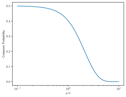
Figure 8: Symmetric cross-over probability induced by hypothesis testing problem for noisy singleton identification/detection.

By invoking (Scarlett & Johnson, 2020), we immediately have the following lemma.

Lemma B.6.

For any fixed SNR, taking $\mathbf{D}_{c}$ such that each element is $\operatorname{Bern}\left(\frac{\nu}{t}\right)$, and $t=\Theta(n^{\alpha})$ for $\alpha\in(0,1)$, taking $P_{1}=O(t\log(n))$ suffices to ensure that the DD algorithm has with vanishing error in the limit as $n\rightarrow\infty$.

B.7.4 Singleton Detection in i.i.d. Spectral Noise

We note that the general flow of this proof follows (Erginbas et al., 2023), but there are several fundamental differences that make this proof overall quite different. We define $\mathcal{E}_{b}$ as the error event where a bin $\mathbf{k}$ is decoded wrongly, and then using a union bound over different bins and different iterations, the probability of the algorithm making a mistake in bin identification satisfies

$$\mathrm{Pr}(\mathcal{E})\leq\text{(\# of iterations)}\times\text{(\# of bins)}\times\mathrm{Pr}(\mathcal{E}_{b})$$

The number of bins is at most $\eta K$ for some constant $\eta$ and the number of iterations is at most $CK$ (at least one edge is peeled off at each iteration in the worst case). Hence, $\mathrm{Pr}(\mathcal{E})\leq\eta CK^{2}\mathrm{Pr}(\mathcal{E}_{b})$. In order to satisfy $\mathrm{Pr}(\mathcal{E})\leq O(1/K)$, we need to show that $\mathrm{Pr}(\mathcal{E}_{b})\leq O(1/K^{3})$.

We already showed in Lemma B.6 that we can achieve singleton identification under noise with vanishing error as $n\to\infty$ with a delay matrix $\mathbf{D}\in\mathbb{Z}_{2}^{P_{1}\times n}$.

To achieve type detection, we construct another pair of delay matrices $\mathbf{D}^{1}\in\mathbb{Z}_{2}^{P_{2}\times n}$ and $\mathbf{D}^{2}\in\mathbb{Z}_{2}^{P_{2}\times n}$. We will choose $\mathbf{D}^{1}$ and $\mathbf{D}^{2}$ such that each element is drawn i.i.d. as a $\operatorname{Bern}\left((1/2)^{1/t}\right)$. We denote the $i^{th}$ row of $\mathbf{D}^{1}$ as $\mathbf{d}_{i}^{1}$ and denote the $i^{th}$ row of $\mathbf{D}^{2}$ as $\mathbf{d}_{i}^{2}$. Then, with these delay matrices, we can obtain observations of the form

$$U_{i}^{1}(\mathbf{k}) =\sum_{\begin{subarray}{c}\mathbf{H}\mathbf{r}=\mathbf{k}\\ \mathbf{r}\leq\mathbf{\overline{d}}_{i}^{1}\end{subarray}}F(\mathbf{r})+Z_{i}(\mathbf{k})$$

$$U_{i}^{2}(\mathbf{k}) =\sum_{\begin{subarray}{c}\mathbf{H}\mathbf{r}=\mathbf{k}\\ \mathbf{r}\leq\mathbf{\overline{d}}_{i}^{2}\end{subarray}}F(\mathbf{r})+Z_{i}(\mathbf{k}).$$

Note that we can represent these observations as

$$\mathbf{U}^{1}=\mathbf{S}^{1}\bm{\alpha}+\mathbf{W}^{1}$$

$$\mathbf{U}^{2}=\mathbf{S}^{2}\bm{\alpha}+\mathbf{W}^{2}$$

with $\mathbf{W}^{1},\mathbf{W}^{2}\sim\mathcal{N}(0,\sigma^{2}\mathbf{I})$, a $\bm{\alpha}$ vector with entries $F(\mathbf{r})$ for coefficients in the set and binary signature matrices $\mathbf{S}^{1},\mathbf{S}^{2}$ with entries indicating the subsets of coefficients included in each sum.

Then, we subtract these observations to obtain a single observation $\mathbf{U}=\mathbf{U}^{1}-\mathbf{U}^{2}$ which can be written as

$$\mathbf{U}=\mathbf{S}\bm{\alpha}+\mathbf{W}$$

with $\mathbf{W}\sim\mathcal{N}(0,2\sigma^{2}\mathbf{I})$ and $\mathbf{S}=\mathbf{S}^{1}-\mathbf{S}^{2}$. This construction allows us to show that the columns of $\mathbf{S}$ are sufficiently incoherent and hence we can correctly perform identification.

Lemma B.7.

For any fixed SNR, taking $\mathbf{D}_{c}^{1}$ and $\mathbf{D}_{c}^{2}$ such that each element is $\operatorname{Bern}\left((1/2)^{1/t}\right)$, and $t=\Theta(n^{\alpha})$ for $\alpha\in(0,1/2)$ and taking $P_{2}=O(t\log(n))$ suffices to ensure that the probability $\mathrm{Pr}(\mathcal{E}_{b})$ for an arbitrary bin can be upper bounded as $\mathrm{Pr}(\mathcal{E}_{b})\leq O(1/K^{3})$.

Proof.

In the following, we prove that $\mathrm{Pr}(\mathcal{E}_{b})\leq O(1/K^{3})$ holds using the observation model. We consider separate cases where the bin in consideration is fixed as a zeroton, singleton, or multiton.

The error probability $\mathrm{Pr}(\mathcal{E}_{b})$ for an arbitrary bin can be upper bounded as

$$\mathrm{Pr}(\mathcal{E}_{b})\leq \sum_{\mathcal{F}\in\{\mathcal{H}_{Z},\mathcal{H}_{M}\}}\mathrm{Pr}(\mathcal{F}\leftarrow\mathcal{H}_{S}(\mathbf{r},F(\mathbf{r})))$$

$$+ \sum_{\mathcal{F}\in\{\mathcal{H}_{Z},\mathcal{H}_{M}\}}\mathrm{Pr}(\mathcal{H}_{S}(\widehat{\mathbf{r}},\widehat{F}(\mathbf{r}))\leftarrow\mathcal{F})$$

$$+ \mathrm{Pr}(\mathcal{H}_{S}(\widehat{\mathbf{r}},\widehat{F}(\mathbf{r}))\leftarrow\mathcal{H}_{S}(\mathbf{r},F(\mathbf{r})))$$

above, each of these events should be read as:

1. $\{\mathcal{F}\leftarrow\mathcal{H}_{S}(\mathbf{r},F(\mathbf{r}))\}$: missed verification in which the singleton verification fails when the ground truth is in fact a singleton.

2. $\{\mathcal{H}_{S}(\widehat{\mathbf{r}},\widehat{F}(\mathbf{r}))\leftarrow\mathcal{F}\}$: false verification in which the singleton verification is passed when the ground truth is not a singleton.

3. $\{\mathcal{H}_{S}(\widehat{\mathbf{r}},\widehat{F}(\mathbf{r}))\leftarrow\mathcal{H}_{S}(\mathbf{r},F(\mathbf{r}))\}$: crossed verification in which a singleton with a wrong index-value pair passes the singleton verification when the ground truth is another singleton pair.

We can upper-bound each of these error terms using Propositions B.8, B.9, and B.10. Note that all upper-bound terms decay exponentially with $P_{2}$ except for the term $\mathrm{Pr}(\widehat{\mathbf{r}}\neq\mathbf{r})\leq O(1/K^{3})$.

We use Theorem 68 to show that we can achieve $\mathrm{Pr}(\widehat{\mathbf{r}}\neq\mathbf{r})\leq O(1/K^{3})$ if we choose $P_{1}=O(t\log n)$. Since all other error probabilities decay exponentially with $P_{2}$, it is clear that if $P_{2}$ is chosen as $P_{2}=O(t\log n)$, the error probability can be bounded as $\mathrm{Pr}(\mathcal{E}_{b})\leq O(1/K^{3})$.

∎

Proposition B.8 (False Verification Rate).

For $0<\gamma<\frac{\eta}{4}\mathrm{SNR}$, the false verification rate for each bin hypothesis satisfies:

$$\mathrm{Pr}(\mathcal{H}_{S}(\widehat{\mathbf{r}},\widehat{F}(\widehat{\mathbf{r}}))\leftarrow\mathcal{H}_{Z}) \leq e^{-\frac{P_{2}}{2}(\sqrt{1+2\gamma}-1)^{2}},$$

$$\mathrm{Pr}(\mathcal{H}_{S}(\widehat{\mathbf{r}},\widehat{F}(\widehat{\mathbf{r}}))\leftarrow\mathcal{H}_{M}) \leq e^{-\frac{P_{2}\gamma^{2}}{4(1+4\gamma)}}+K^{2}e^{-\epsilon\left(1-\frac{4\gamma\nu^{2}}{\rho^{2}}\right)^{2}P_{2}},$$

where $P_{2}$ is the number of the random offsets.

Proof.

The probability of detecting a zeroton as a singleton can be upper-bounded by the probability of a zeroton failing the zeroton verification. This means

$$\mathrm{Pr}(\mathcal{H}_{S}(\widehat{\mathbf{r}},\widehat{F}(\widehat{\mathbf{r}}))\leftarrow\mathcal{H}_{Z}) \leq\mathrm{Pr}\left(\frac{1}{P_{2}}\|\mathbf{W}\|^{2}\geq(1+\gamma)\nu^{2}\right)$$

$$\leq e^{-\frac{P_{2}}{4}(\sqrt{1+2\gamma}-1)^{2}},$$

by noting that $\mathbf{W}\sim\mathcal{N}(0,\nu^{2}\mathbf{I})$ and applying Lemma B.11.

On the other hand, given some multiton observation $\mathbf{U}=\mathbf{S}\bm{\alpha}+\mathbf{W}$, the probability of detecting it as a singleton with index-value pair $(\widehat{\mathbf{r}},\widehat{F}(\widehat{\mathbf{r}}))$ can be written as

$$\mathrm{Pr}(\mathcal{H}_{S}(\widehat{\mathbf{r}},\widehat{F}(\widehat{\mathbf{r}}))\leftarrow\mathcal{H}_{M})=\mathrm{Pr}\left(\frac{1}{P_{2}}\left\|\mathbf{U}-\widehat{F}(\widehat{\mathbf{r}})\mathbf{s}_{\widehat{\mathbf{r}}}\right\|^{2}\leq(1+\gamma)\nu^{2}\right)=\mathrm{Pr}\left(\frac{1}{P_{2}}\left\|\mathbf{g}+\mathbf{v}\right\|^{2}\leq(1+\gamma)\nu^{2}\right),$$

where $\mathbf{g}:=\mathbf{S}(\bm{\alpha}-\widehat{F}(\widehat{\mathbf{r}})\mathbf{e}_{\widehat{\mathbf{r}}})$ and $\mathbf{v}:=\mathbf{W}$. Then, we can upper bound this probability as

$$\mathrm{Pr}\left(\frac{1}{P_{2}}\left\|\mathbf{g}+\mathbf{v}\right\|^{2}\leq(1+\gamma)\nu^{2}\middle|\frac{\|\mathbf{g}\|^{2}}{P_{2}}\geq 2\gamma\nu^{2}\right)+\mathrm{Pr}\left(\frac{\|\mathbf{g}\|^{2}}{P_{2}}\leq 2\gamma\nu^{2}\right).$$

To upper bound the first term, we use Lemma B.11. Note that the first term is conditioned on the event $\|\mathbf{g}\|^{2}/P_{2}\geq 2\gamma\nu^{2}$, thus the normalized non-centrality parameter satisfies $\theta_{0}\geq 2\gamma$. As a result, we can use Lemma B.11 by letting $\tau_{2}=(1+\gamma)\nu^{2}$. Then, the first term is upper bounded by $\exp\{-(P_{2}\gamma^{2})/(4(1+4\gamma))\}$. To analyze the second term, we let $\bm{\beta}=\bm{\alpha}-\widehat{F}(\widehat{\mathbf{r}})\mathbf{e}_{\widehat{\mathbf{r}}}$ and write $\mathbf{g}=\mathbf{S}\bm{\beta}$. Denoting its support as $\mathcal{L}:=\mathrm{supp}(\bm{\beta})$, we can further write $\mathbf{S}\bm{\beta}=\mathbf{S}_{\mathcal{L}}\bm{\beta}_{\mathcal{L}}$ where $\mathbf{S}_{\mathcal{L}}$ is the sub-matrix of $\mathbf{S}$ consisting of the columns in $\mathcal{L}$ and $\bm{\beta}_{\mathcal{L}}$ is the sub-vector consisting of the elements in $\mathcal{L}$. Then, we consider two scenarios:

• The multiton size is a constant, i.e., $|\mathcal{L}|=L=O(1)$. In this case, we have

  $$\lambda_{\mathrm{min}}(\mathbf{S}_{\mathcal{L}}^{\top}\mathbf{S}_{\mathcal{L}})\|\bm{\beta}_{\mathcal{L}}\|^{2}\leq\|\mathbf{S}_{\mathcal{L}}\bm{\beta}_{\mathcal{L}}\|^{2}$$

  Using $\|\bm{\beta}_{\mathcal{L}}\|^{2}\geq L\rho^{2}$, the probability can be bounded as

  $$\mathrm{Pr}\left(\frac{\|\mathbf{g}\|^{2}}{P_{2}}\leq 2\gamma\nu^{2}\right)\leq\mathrm{Pr}\left(\lambda_{\mathrm{min}}\left(\frac{1}{P_{2}}\mathbf{S}_{\mathcal{L}}^{\top}\mathbf{S}_{\mathcal{L}}\right)\leq\frac{2\gamma\nu^{2}}{L\rho^{2}}\right)$$

  On the other hand, using Lemma B.12 with the selection $\beta=1/2$ and $\eta=\frac{1}{1+2L}(\frac{1}{2}-\frac{2\gamma\nu^{2}}{L\rho^{2}})$, we have

  $$\mathrm{Pr}\left(\frac{\|\mathbf{g}\|^{2}}{P_{2}}\leq 2\gamma\nu^{2}\right)\leq 2L^{2}e^{-\frac{P_{2}}{2(1+2L)^{2}}\left(\frac{1}{2}-\frac{2\gamma\nu^{2}}{L\rho^{2}}\right)^{2}}.$$

  which holds as long as $\gamma<L\rho^{2}/(4\nu^{2})=\frac{L\eta}{4}\mathrm{SNR}$.

• The multiton size grows asymptotically with respect to $K$, i.e., $|\mathcal{L}|=L=\omega(1)$. As a result, the vector of random variables $\mathbf{g}=\mathbf{S}_{\mathcal{L}}\bm{\beta}_{\mathcal{L}}$ becomes asymptotically Gaussian due to the central limit theorem with zero mean and a covariance

  $$\mathbb{E}[\mathbf{g}\mathbf{g}^{\mathrm{H}}]=\frac{1}{2}L\rho^{2}\mathbf{I}$$

  Therefore, by Lemma B.11, we have

  $$\mathrm{Pr}\left(\frac{\|\mathbf{g}\|^{2}}{P_{2}}\leq 2\gamma\nu^{2}\right)\leq e^{-\frac{P_{2}}{2}\left(1-\frac{\gamma\nu^{2}}{L\rho^{2}}\right)}$$

  which holds as long as $\gamma<L\rho^{2}/\nu^{2}=L\eta\mathrm{SNR}$.

By combining the results from both cases, there exists some absolute constant $\epsilon>0$ such that

$$\mathrm{Pr}\left(\frac{\|\mathbf{g}\|^{2}}{P_{2}}\leq 2\gamma\nu^{2}\right)\leq K^{2}e^{-\epsilon\left(1-\frac{4\gamma\nu^{2}}{\rho^{2}}\right)^{2}P_{2}}$$

as long as $\gamma<\rho^{2}/(4\nu^{2})=\frac{\eta}{4}\mathrm{SNR}$. ∎

Proposition B.9 (Missed Verification Rate).

For $0<\gamma<\frac{\eta}{2}\mathrm{SNR}$, the missed verification rate for each bin hypothesis satisfies

$$\mathrm{Pr}(\mathcal{H}_{Z}\leftarrow\mathcal{H}_{S}(\mathbf{r},F[\mathbf{r}])) \leq e^{-\frac{P_{2}}{4}\frac{(\rho^{2}/\nu^{2}-\gamma)^{2}}{1+2\rho^{2}/\nu^{2}}}$$

$$\mathrm{Pr}(\mathcal{H}_{M}\leftarrow\mathcal{H}_{S}(\mathbf{r},F[\mathbf{r}])) \leq e^{-\frac{P_{2}}{4}(\sqrt{1+2\gamma}-1)^{2}}+2e^{-\frac{\rho^{2}}{2\nu^{2}}P_{2}}+2\mathrm{Pr}(\widehat{\mathbf{r}}\neq\mathbf{r})$$

where $P_{2}$ is the number of the random offsets.

Proof.

The probability of detecting a singleton as a zeroton can be upper bounded by the probability of a singleton passing the zeroton verification. Hence, by noting that $\mathbf{W}\sim\mathcal{N}(0,\nu^{2}\mathbf{I})$ and applying Lemma B.11,

$$\mathrm{Pr} (\mathcal{H}_{Z}\leftarrow\mathcal{H}_{S}(\mathbf{r},F[\mathbf{r}]))$$

$$\leq\mathrm{Pr}\left(\frac{1}{P_{2}}\|F[\mathbf{r}]\mathbf{s}_{\mathbf{r}}+\mathbf{W}\|^{2}\leq(1+\gamma)\nu^{2}\right)$$

$$\leq e^{-\frac{P_{2}}{4}\frac{(\rho^{2}/\nu^{2}-\gamma)^{2}}{1+2\rho^{2}/\nu^{2}}}.$$

which holds as long as $\gamma<\rho^{2}/\nu^{2}=\eta\mathrm{SNR}$.

On the other hand, the probability of detecting a singleton as a multiton can be written as the probability of failing the singleton verification step for some index-value pair $(\widehat{\mathbf{r}},\widehat{F}[\widehat{\mathbf{r}}])$. Hence, we can write

$$\mathrm{Pr}(\mathcal{H}_{M}\leftarrow\mathcal{H}_{S}(\mathbf{r},F[\mathbf{r}])) =\mathrm{Pr}\left(\frac{1}{P_{2}}\left\|\mathbf{U}-\widehat{F}[\widehat{\mathbf{r}}]\mathbf{s}_{\widehat{k}}\right\|^{2}\geq(1+\gamma)\nu^{2}\right)$$

$$\leq\mathrm{Pr}\left(\frac{1}{P_{2}}\left\|\mathbf{U}-\widehat{F}[\widehat{\mathbf{r}}]\mathbf{s}_{\widehat{k}}\right\|^{2}\geq(1+\gamma)\nu^{2}\middle|\widehat{F}[\widehat{\mathbf{r}}]=F[\mathbf{r}]\wedge\widehat{\mathbf{r}}=\mathbf{r}\right)+\mathrm{Pr}(\widehat{F}[\widehat{\mathbf{r}}]\neq F[\mathbf{r}]\vee\widehat{\mathbf{r}}\neq\mathbf{r}).$$

Then, using Lemma B.11, the first term is upper-bounded as

$$\mathrm{Pr}\left(\frac{1}{P_{2}}\left\|\mathbf{U}-\widehat{F}[\widehat{\mathbf{r}}]\mathbf{s}_{\widehat{k}}\right\|^{2}\geq(1+\gamma)\nu^{2}\middle|\widehat{F}[\widehat{\mathbf{r}}]=F[\mathbf{r}]\wedge\widehat{\mathbf{r}}=\mathbf{r}\right) \leq\mathrm{Pr}\Big{(}\frac{1}{P_{2}}\|\mathbf{W}\|^{2}\geq(1+\gamma)\nu^{2}\Big{)}$$

$$\leq e^{-\frac{P_{2}}{4}(\sqrt{1+2\gamma}-1)^{2}}.$$

On the other hand, the second term can be bounded as

$$\mathrm{Pr}(\widehat{F}[\widehat{\mathbf{r}}]\neq F[\mathbf{r}]\vee\widehat{\mathbf{r}}\neq\mathbf{r}) \leq\mathrm{Pr}(\widehat{F}[\widehat{\mathbf{r}}]\neq F[\mathbf{r}])+\mathrm{Pr}(\widehat{\mathbf{r}}\neq\mathbf{r})$$

$$=\mathrm{Pr}(\widehat{F}[\widehat{\mathbf{r}}]\neq F[\mathbf{r}]|\widehat{\mathbf{r}}\neq\mathbf{r})\mathrm{Pr}(\widehat{\mathbf{r}}\neq\mathbf{r})$$

$$\qquad+\mathrm{Pr}(\widehat{F}[\widehat{\mathbf{r}}]\neq F[\mathbf{r}]|\widehat{\mathbf{r}}=\mathbf{r})\mathrm{Pr}(\widehat{\mathbf{r}}=\mathbf{r})$$

$$\qquad+\mathrm{Pr}(\widehat{\mathbf{r}}\neq\mathbf{r})$$

$$\leq\mathrm{Pr}(\widehat{F}[\widehat{\mathbf{r}}]\neq F[\mathbf{r}]|\widehat{\mathbf{r}}=\mathbf{r})+2\mathrm{Pr}(\widehat{\mathbf{r}}\neq\mathbf{r})$$

The first term is the error probability of a BPSK signal with amplitude $\rho$, and it can be bounded as

$$\mathrm{Pr}(\widehat{F}[\widehat{\mathbf{r}}]\neq F[\mathbf{r}]|\widehat{\mathbf{r}}=\mathbf{r})\leq 2e^{-\frac{\rho^{2}}{2\nu^{2}}P_{2}}$$

∎

Proposition B.10 (Crossed Verification Rate).

For $0<\gamma<\frac{\eta}{2}\mathrm{SNR}$, the crossed verification rate for each bin hypothesis satisfies

$$\mathrm{Pr}(\mathcal{H}_{S}(\widehat{\mathbf{r}},\widehat{F}[\widehat{\mathbf{r}}])\leftarrow\mathcal{H}_{S}(\mathbf{r},F[\mathbf{r}]))\leq e^{-\frac{P_{2}\gamma^{2}}{4(1+4\gamma)}}+Ke^{-\epsilon\left(1-\frac{4\gamma\nu^{2}}{\rho^{2}}\right)^{2}P_{2}}+K^{2}e^{-\epsilon\left(1-\frac{4\gamma\nu^{2}}{\rho^{2}}\right)^{2}P_{2}^{2}/t}.$$

where $P_{2}$ is the number of the random offsets.

Proof.

This error event can only occur if a singleton with index-value pair $(\mathbf{r},F[\mathbf{r}])$ passes the singleton verification step for some index-value pair $(\widehat{\mathbf{r}},\widehat{F}[\widehat{\mathbf{r}}])$ such that $\mathbf{r}\neq\widehat{\mathbf{r}}$. Hence,

$$\mathrm{Pr}(\mathcal{H}_{S}(\widehat{\mathbf{r}},\widehat{F}[\widehat{\mathbf{r}}])\leftarrow\mathcal{H}_{S}(\mathbf{r},F[\mathbf{r}]))$$

$$\leq\mathrm{Pr}\left(\frac{1}{P_{2}}\|F[\mathbf{r}]\mathbf{s}_{\mathbf{r}}-\widehat{F}[\widehat{\mathbf{r}}]\mathbf{s}_{\widehat{\mathbf{r}}}+\mathbf{W}\|^{2}\leq(1+\gamma)\nu^{2}\right)$$

$$=\mathrm{Pr}\left(\frac{1}{P_{2}}\|\mathbf{S}\bm{\beta}+\mathbf{W}\|^{2}\leq(1+\gamma)\nu^{2}\right)$$

$$=\mathrm{Pr}\left(\frac{1}{P_{2}}\|\mathbf{S}\bm{\beta}+\mathbf{W}\|^{2}\leq(1+\gamma)\nu^{2}\middle|\|\mathbf{S}\bm{\beta}\|^{2}\geq 2\gamma\nu^{2}\right)$$

$$\qquad+\mathrm{Pr}\left(\|\mathbf{S}\bm{\beta}\|^{2}\leq 2\gamma\nu^{2}\right)$$

where $\bm{\beta}$ is a $2$-sparse vector with non-zero entries from $\{\rho,-\rho\}$. Using Lemma B.11, the first term is upper-bounded as

$$\mathrm{Pr}\left(\frac{1}{P_{2}}\|\mathbf{S}\bm{\beta}+\mathbf{W}\|^{2}\leq(1+\gamma)\nu^{2}\middle|\|\mathbf{S}\bm{\beta}\|^{2}\geq 2\gamma\nu^{2}\right)\leq e^{-\frac{P_{2}\gamma^{2}}{4(1+4\gamma)}}.$$

By Lemma B.12, the second term is upper bounded as

$$\mathrm{Pr}\left(\|\mathbf{S}\bm{\beta}\|^{2}\leq 2\gamma\nu^{2}\right)\leq 8e^{-\frac{P_{2}}{50}\left(\frac{1}{2}-\frac{\gamma\nu^{2}}{L\rho^{2}}\right)^{2}}$$

which holds as long as $\gamma<\rho^{2}/(2\nu^{2})=\frac{\eta}{2}\mathrm{SNR}$.

∎

Lemma B.11 (Non-central Tail Bounds (Lemma 11 in (Li et al., 2014))).

Given any $\mathbf{g}\in\mathbb{R}^{P}$ and a Gaussian vector $\mathbf{v}\sim\mathcal{N}(0,\nu^{2}\mathbf{I})$, the following tail bounds hold:

$$\mathrm{Pr}\left(\frac{1}{P}\|\mathbf{g}+\mathbf{v}\|^{2}\geq\tau_{1}\right) \leq e^{-\frac{P}{4}(\sqrt{2\tau_{1}/\nu^{2}-1}-\sqrt{1+2\theta_{0}})^{2}}$$

$$\mathrm{Pr}\left(\frac{1}{P}\|\mathbf{g}+\mathbf{v}\|^{2}\leq\tau_{2}\right) \leq e^{-\frac{P}{4}\frac{\left(1+\theta_{0}-\tau_{2}/\nu^{2}\right)^{2}}{1+2\theta_{0}}}$$

for any $\tau_{1}$ and $\tau_{2}$ that satisfy $\tau_{1}\geq\nu^{2}(1+\theta_{0})\geq\tau_{2}$ where

$$\theta_{0}:=\frac{\|\mathbf{g}\|^{2}}{P\nu^{2}}$$

is the normalized non-centrality parameter.

Lemma B.12.

Suppose $\beta=\Theta(1)$, $\eta=\Omega(1)$, and $t=\Theta(n^{\alpha})$ for some $\alpha\in(0,1/2)$. Then, there exists some $n_{0}$ such that for all $n\geq n_{0}$, we have

$$\Pr\left(\lambda_{\mathrm{min}}\left(\frac{1}{P_{2}}\mathbf{S}_{\mathcal{L}}^{\top}\mathbf{S}_{\mathcal{L}}\right)\leq 2\beta(1-\beta)-(2L+1)\eta\right)\leq 2L^{2}\exp\left(-\frac{\eta^{2}}{2}P_{2}\right).$$

Proof.

For any $\mathbf{r}$ sampled uniformly from vectors up to degree $t$, the probability that it will have degree $0\leq k\leq t$ can be written as

$$\Pr\left(|\mathbf{r}|=k\right)=\frac{\binom{n}{k}}{\sum_{k=1}^{t}{\binom{n}{k}}}$$

We know that the entries of $\mathbf{s}_{\mathbf{r}}$ are given as $(\mathbf{s}_{\mathbf{r}}^{1})_{i}=\mathds{1}\left\{\mathbf{r}\leq\bar{\mathbf{d}}_{i}^{1}\right\}$ and $(\mathbf{s}_{\mathbf{r}}^{2})_{i}=\mathds{1}\left\{\mathbf{r}\leq\bar{\mathbf{d}}_{i}^{2}\right\}$. Therefore,

$$\Pr\left((\mathbf{s}_{\mathbf{r}}^{1})_{i}=1\right) =\Pr\left(d_{ij}^{1}=0,\forall j\in\mathrm{supp}(\mathbf{r})\right)$$

$$=\sum_{k=1}^{t}\Pr\left(d_{ij}^{1}=0,\forall j\in\mathrm{supp}(\mathbf{r})||\mathbf{r}|=k\right)\Pr\left(|\mathbf{r}|=k\right)$$

$$=\frac{\sum_{k=1}^{t}{\binom{n}{k}}\beta^{k/t}}{\sum_{k=1}^{t}{\binom{n}{k}}}.$$

$$=:g(t,n)$$

With $\beta=\Theta(1)$ and $t=\Theta(n^{\alpha})$ for $\alpha\in(0,1/2)$, we can show that $\lim_{n\to\infty}g(t,n)=\beta$. Therefore, there exists some $n_{0}$ such that $|\Pr\left((\mathbf{s}_{\mathbf{r}}^{1})_{i}=1\right)-\beta|\leq\eta$ for all $n\geq n_{0}$. For the rest of the proof, let $g=\Pr\left((\mathbf{s}_{\mathbf{r}}^{1})_{i}=1\right)$ and assume $|g-\beta|\leq\eta$.

Then, recalling $(\mathbf{s}_{\mathbf{r}})_{i}=(\mathbf{s}_{\mathbf{r}}^{1})_{i}-(\mathbf{s}_{\mathbf{r}}^{2})_{i}$, the distribution for each entry of $\mathbf{s}_{\mathbf{r}}$ can be written as

$$\Pr\left((\mathbf{s}_{\mathbf{r}})_{i}=1\right) =\Pr\left((\mathbf{s}_{\mathbf{r}})_{i}=-1\right)=g(1-g).$$

Hence, using Hoeffding’s inequality, we obtain

$$\Pr\left(\frac{1}{P_{2}}\mathbf{s}_{\mathbf{r}}^{\top}\mathbf{s}_{\mathbf{r}}\leq 2\beta(1-\beta)-\eta\right)\leq\Pr\left(\frac{1}{P_{2}}\mathbf{s}_{\mathbf{r}}^{\top}\mathbf{s}_{\mathbf{r}}\leq 2g(1-g)-\eta\right)\leq\exp\left(-\frac{\eta^{2}}{2}P_{2}\right).$$

Furthermore, the conditional probability of another vector $\mathbf{m}\neq\mathbf{r}$ being included in test $i$ is given by

$$\Pr\left((\mathbf{s}_{\mathbf{m}}^{1})_{i}=1|(\mathbf{s}_{\mathbf{r}}^{1})_{i}=1,|\mathbf{r}|=k\right) =\Pr\left(d_{ij}=0,\forall j\in\mathrm{supp}(\mathbf{m})\setminus\mathrm{supp}(\mathbf{r})||\mathbf{r}|=k\right)$$

$$=\sum_{\ell=0}^{t}\left(\beta^{1/t}\right)^{\ell}\left(1-\frac{k}{n}\right)^{\ell}\left(\frac{k}{n}\right)^{t-\ell}$$

$$=\left(\frac{k}{n}+\left(1-\frac{k}{n}\right)\beta^{1/t}\right)^{t}$$

$$=:f(t,n,k).$$

With $\beta=\Theta(1)$ and $t=\Theta(n^{\alpha})$ for $\alpha\in(0,1)$, for any $k\leq t$, we can show that $\lim_{n\to\infty}f(t,n,k)=\beta$. Therefore, there exists some $n_{0}$ such that $|\Pr\left((\mathbf{s}_{\mathbf{m}}^{1})_{i}=1|(\mathbf{s}_{\mathbf{r}}^{1})_{i}=1\right)-\beta|\leq\eta$ for all $n\geq n_{0}$. For the rest of the proof, let $f=\Pr\left((\mathbf{s}_{\mathbf{m}}^{1})_{i}=1|(\mathbf{s}_{\mathbf{r}}^{1})_{i}=1\right)$ and assume $|f-\beta|\leq\eta$.

On the other hand,

$$\Pr\left((\mathbf{s}_{\mathbf{m}})_{i}(\mathbf{s}_{\mathbf{r}})_{i}=1\right) =2fg\left[1-g-(1-f)g\right]$$

$$\Pr\left((\mathbf{s}_{\mathbf{m}})_{i}(\mathbf{s}_{\mathbf{r}})_{i}=-1\right) =2\left[(1-f)g\right]^{2}$$

As a result, we have

$$\mathbb{E}[(\mathbf{s}_{\mathbf{m}})_{i}(\mathbf{s}_{\mathbf{r}})_{i}]=2g(f-g).$$

Since $\lim_{n\to\infty}\mathbb{E}[(\mathbf{s}_{\mathbf{m}})_{i}(\mathbf{s}_{\mathbf{r}})_{i}]=0$, there exists some $n_{0}$ such that $-\eta\leq\mathbb{E}[(\mathbf{s}_{\mathbf{m}})_{i}(\mathbf{s}_{\mathbf{r}})_{i}]\leq\eta$ for all $n\geq n_{0}$. For the rest of the proof assume $-\eta\leq\mathbb{E}[(\mathbf{s}_{\mathbf{m}})_{i}(\mathbf{s}_{\mathbf{r}})_{i}]\leq\eta$. As a result, we can write

$$\Pr\left(\frac{1}{P_{2}}|\mathbf{s}_{\mathbf{r}}^{\top}\mathbf{s}_{\mathbf{m}}|\geq 2\eta\right)\leq\Pr\left(|\mathbf{s}_{\mathbf{r}}^{\top}\mathbf{s}_{\mathbf{m}}-P_{2}\mathbb{E}[(\mathbf{s}_{\mathbf{m}})_{i}(\mathbf{s}_{\mathbf{r}})_{i}]|\geq P_{2}\eta\right)\leq\exp\left(-\frac{\eta^{2}}{2}P_{2}\right).$$

By Gershgorin Circle Theorem, the minimum eigenvalue of $\frac{1}{P_{2}}\mathbf{S}_{\mathcal{L}}^{\top}\mathbf{S}_{\mathcal{L}}$ is lower bounded as

$$\lambda_{\mathrm{min}}\left(\frac{1}{P_{2}}\mathbf{S}_{\mathcal{L}}^{\top}\mathbf{S}_{\mathcal{L}}\right)\geq\frac{1}{P_{2}}\min_{\mathbf{r}\in\mathcal{L}}\left(|\mathbf{s}_{\mathbf{r}}^{\top}\mathbf{s}_{\mathbf{r}}|-\sum_{\begin{subarray}{c}\mathbf{m}\in\mathcal{L}\\ \mathbf{m}\neq\mathbf{r}\end{subarray}}|\mathbf{s}_{\mathbf{r}}^{\top}\mathbf{s}_{\mathbf{m}}|\right).$$

Lastly, we apply a union bound over all $(\mathbf{r},\mathbf{m})$ pairs to obtain

$$\Pr\left(\lambda_{\mathrm{min}}\left(\frac{1}{P_{2}}\mathbf{S}_{\mathcal{L}}^{\top}\mathbf{S}_{\mathcal{L}}\right)\leq 2\beta(1-\beta)-(2L+1)\eta\right)\leq 2L^{2}\exp\left(-\frac{\eta^{2}}{2}P_{2}\right).$$

∎

Appendix C Worst-Case Time Complexity

In this section, we discuss the computational complexity of Algorithm 1, which is broken down into the following parts:

Computing Samples

Computing samples for one sapling matrix requires computing the row-span of $\mathbf{H}_{c}$, which can be computed in $n2^{b}$ operations. Then for each sample, we must take the bit-wise and with each row of the delay matrix, so the total complexity is: $Cn2^{b}P$.

Taking Small Mobius Transform

Computing the Mobius transform for each of the $CP$ subsampled functions is $CPb2^{b}$.

Singleton Detection

To detect each singleton requires computing $\mathbf{y}$. This requires $P$ divisions for each of the $C2^{b}$ bins, for a total of $CP2^{b}$ operations.

Singleton Identification

To identify each singleton requires different complexity for our different assumptions.

1. In the case of uniformly distributed interactions, singleton detection is $O(1)$, since $\mathbf{y}=\mathbf{k}^{*}$ immediately, so doing this for each singleton makes the total complexity $CK$.

2. In the noiseless low-degree case decoding $\mathbf{k}^{*}$ from $\mathbf{y}$ is $\operatorname{poly}(n)$, so for each singleton the complexity is $CK\operatorname{poly}(n)$

Message Passing

In the worst case, we peel exactly one singleton per iteration, resulting in $CK$ subtractions (the above singleton identification bounds already take into account the need to re-do singelton identification).

Thus in the case of uniformly distributed and low-degree interactions respectively, the complexity is:

Uniform distributed noiseless time complexity $$= O(CPn2^{b}+CPb2^{b}+CK)$$

$$= O(CPnK)$$

$$= O(n^{2}K).$$

Low-degree (noisy) time complexity $$= O(CPn2^{b}+CPb2^{b}+CK\operatorname{poly}(n))$$

$$= O(CP\operatorname{poly}(n)K)$$

$$= O(\operatorname{poly}(n)K).$$

Appendix D Additional Simulations

In this section, we present some additional simulations that did not fit in the body of the manuscript. Fig 9 and 10. Plot the runtime of SMT vs. $n$ under both of our assumptions. In both cases we observe excellent scaling with $n$. We note that our low-degree setting has a higher fixed cost since we are using linear programming to solve our group testing problem and the solver appears to have some non-trivial fixed time cost.

Fig. 11 plots the perfect reconstruction percentage against $n$ and sample complexity. We also observe a phase transition, however, the phase threshold appears very insensitive to $n$, as expected, since our sample complexity requirement is growing like $\log(n)$, and we are already plotting on a log scale.

Figure 9: Time complexity of SMT under Assumption 3.1. The parameter $K$ is fixed and we plot the runtime v.s. $n$. our algorithm remains possible to run for $n=1000$ where other competitors fail.

Figure 10: Time complexity of SMT under assumption  3.2. The parameters $K$ and $t$ are fixed and we plot the runtime v.s. $n$. Our theory says we have a $\operatorname{poly}(n)$ complexity. In practice, for reasonable $n$ our algorithm is running quickly.

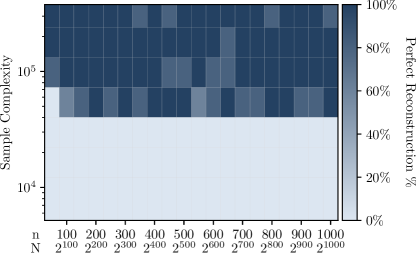
Figure 11: Perfect reconstruction percentage plotted against sample complexity and $n$ under Assumption 3.2. Holding $C=3$, we scale $b$ to increase the sample complexity. We observe that the number of samples required to achieve perfect reconstruction is scaling linearly is very insensitive to $n$ as predicted. We also include $N=2^{n}$ on the bottom axis, which is the total number of interactions. In this regime we do not appear to consistently maintain zero error. This could be due to the fact that the asymptotic behaviour of group testing might not yet be fuly realized in the regime with $n\leq 1000$.

		Arbitrary	Paths	Proximity
Small Regime	Mobius	$13.5\pm 10.1$	$5.8\pm 5.9$	$9.9\pm 8.2$
	Fourier	$(3.4\pm 3.9)\times 10^{5}$	$2{,}231.2\pm 4{,}872.3$	$(3.2\pm 4.2)\times 10^{5}$
Large Regime	Mobius	$13.3\pm 10.4$	$5.7\pm 3.9$	$10.8\pm 8.9$
	Samples	$(1.8\pm 1.8)\times 10^{5}$	$(1.7\pm 2.0)\times 10^{5}$	$(1.9\pm 2.1)\times 10^{5}$
	Time (s)	$0.72\pm 0.57$	$0.34\pm 0.27$	$0.63\pm 0.54$

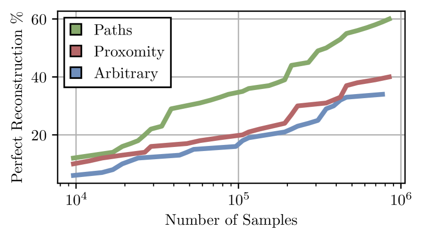
Figure 12: (Left) In cases of perfect recovery, mean $\pm$ standard deviation of the sparsity and performance of SMT across the Arbitrary, Paths, and Proxmity settings from (Leyton-Brown et al., 2000). The Mobius sparsity does not grow with the number of items. (Right) Across 100 realizations of each setting, the number of realizations that are perfectly recoverable by the SMT algorithm for a given number samples. On these three distributions, perfect recovery is not achievable in $10^{6}$ samples on all realizations by the Sparse Mobius Transform.

Finally, we discuss a few additional combinatorial auction settings in Fig. 12. In these settings SMT requires too many samples for accurate construction. The main reason is that in these settings, interactions between inputs are very correlated and the distribution of the degrees is very strange, and difficult to uniformly hash accross the aliasing sets. The algorithm and techniques used in SMT are a clear step forward in state of the art methods for computing interaction scores in many ways, and many of our theoretical assumptions can be relaxed in practice. Some of our assumptions, however, cannot be relaxed in practice. Many problems like these have correlated interactions and future iterations of this algorithm should try to resolve these issues.

Appendix E Group Testing

E.1 Group Testing Achievability Results From Literature

Theorem E.1 (Part of Theorem 4.1 and 4.2 in Aldridge et al. (2019)).

Asymptotic Rate 1 Noiseless Group Testing: Consider a noiseless group testing problem with $t=\Theta(n^{\theta})$ defects out of $n$ elements. We define the rate of a group testing procedure as:

$$R\vcentcolon=\frac{\log\binom{n}{t}}{T}$$ (62)

where $T$ is the number of tests performed by the group testing procedure. For an i.i.d. Bernoulli design matrix, for $\theta\in[0,1/3]$, in the limit as $n\rightarrow\infty$, a rate $R^{*}_{\text{BERN}}=1$ is achievable with vanishing error. Furthermore, for the constant column-weight design matrix, for $\theta\in[0,0.409]$ a rate $R^{*}_{\text{CCW}}=1$ is achievable with vanishing error.

Theorem E.2 (Bay et al. (2022)).

Noiseless Group Testing: Consider the noiseless non-adaptive group testing setup with $t=\left\lvert\mathbf{k}\right\rvert$ defects out of $n$ items, with $t$ scaling arbitrarily in $n$. Let $\hat{\mathbf{k}}$ be the output of a group testing decoder and let $T^{*}=\Theta\left(\min\left\{t\log(n),n\right\}\right)$. Then there exists a strategy using $T\leq(1+\epsilon)T^{*}$ such that in the limit as $n\rightarrow\infty$ we have:

$$\Pr\left(\hat{\mathbf{k}}\neq\mathbf{k}\right)\rightarrow 0.$$ (63)

Furthermore, there is a $\operatorname{poly}(n)$ algorithm for computing $\hat{\mathbf{k}}$.

Theorem E.3 ((Scarlett & Johnson, 2020)).

Noisy Group Testing Under General Binary Noise: Consider the general binary noisy group testing setup with crossover probabilities $p_{10}$ and $p_{01}$. We use i.i.d Bernoulli testing with parameter $\nu>0$. There are a total of $\left\lvert\mathbf{k}\right\rvert=t=\Theta(n^{\theta})$ defects, where $\theta\in(0,1)$. Let $T^{*}=\max\left\{T_{1}^{(D)},T_{1}^{(ND)},T_{2}^{(D)},T_{2}^{(ND)}\right\}$, where we have

$$T_{1}^{(D)} = \frac{1}{\nu p_{10}D_{(}\alpha/p_{10})}t\log(t),$$ (64)

$$T_{1}^{(ND)} = \frac{1}{\nu wD(\alpha/w)}t\log(n),$$ (65)

$$T_{2}^{(D)} = \frac{1}{\nu e^{-\nu}(1-p_{10})D(\beta/p_{10})}t\log(t),$$ (66)

$$T_{2}^{(ND)} = \frac{1}{\nu p_{01}D(\beta/p_{01})}t\log(n).$$ (67)

where $D(x)=x\log(x)-x+1$, and $w=(1-p_{01})e^{-\nu}+p_{10}(1-e^{-\nu})$. For any $\alpha\in(p_{10},1-p_{01})$, $\beta\in(p_{01},1-p_{10})$, there exist some number of tests $T<(1+\epsilon)T^{*}$ where the Noisy DD algorithm produces $\hat{\mathbf{k}}$ such that in the limit as $n\rightarrow\infty$ we have:

$$\Pr\left(\hat{\mathbf{k}}\neq\mathbf{k}\right)\rightarrow 0.$$ (68)

E.2 Group Testing Implementation

We implement group testing via linear programming. As noted in (Aldridge et al., 2019), linear programming generally outperforms most other group testing algorithms in both the noisy and noiseless case. We use the following linear program, to implement group testing.

$$\min_{\mathbf{k},\bm{\xi}} \sum_{i=1}^{n}k_{i}+\lambda\sum_{p=1}^{P}{\xi_{j}}$$ (69)

s.t. $$k_{i}\geq 0$$

$$\xi_{p}\geq 0$$

$$\xi_{p}\leq 1\quad p\text{ s.t. }y_{p}=1$$

$$\mathbf{d}_{p}^{\textrm{T}}\mathbf{k}=\xi_{p}\quad p\text{ s.t. }y_{p}=0$$

$$\mathbf{d}_{p}^{\textrm{T}}\mathbf{k}+\xi_{p}\geq 1\quad p\text{ s.t. }y_{p}=1$$

References

- Aldridge et al. (2019) Aldridge, M., Johnson, O., and Scarlett, J. Group testing: An information theory perspective. Foundations and Trends® in Communications and Information Theory, 15(3–4):196–392, 2019. ISSN 1567-2328. doi: 10.1561/0100000099. URL http://dx.doi.org/10.1561/0100000099.
- Amrollahi et al. (2019) Amrollahi, A., Zandieh, A., Kapralov, M., and Krause, A. Efficiently learning fourier sparse set functions. Advances in Neural Information Processing Systems, 32, 2019.
- Bay et al. (2022) Bay, W. H., Scarlett, J., and Price, E. Optimal non-adaptive probabilistic group testing in general sparsity regimes. Information and Inference: A Journal of the IMA, 11(3):1037–1053, 02 2022. ISSN 2049-8772. doi: 10.1093/imaiai/iaab020. URL https://doi.org/10.1093/imaiai/iaab020.
- Chung et al. (2001) Chung, S.-Y., Richardson, T., and Urbanke, R. Analysis of sum-product decoding of low-density parity-check codes using a gaussian approximation. IEEE Transactions on Information Theory, 47(2):657–670, 2001. doi: 10.1109/18.910580.
- Coja-Oghlan et al. (2020) Coja-Oghlan, A., Gebhard, O., Hahn-Klimroth, M., and Loick, P. Information-theoretic and algorithmic thresholds for group testing. IEEE Transactions on Information Theory, 66(12):7911–7928, 2020. doi: 10.1109/TIT.2020.3023377.
- Conen & Sandholm (2001) Conen, W. and Sandholm, T. Preference elicitation in combinatorial auctions. In Proceedings of the 3rd ACM Conference on Electronic Commerce, pp. 256–259, 2001.
- Devlin et al. (2019) Devlin, J., Chang, M.-W., Lee, K., and Toutanova, K. Bert: Pre-training of deep bidirectional transformers for language understanding. In North American Chapter of the Association for Computational Linguistics, 2019. URL https://api.semanticscholar.org/CorpusID:52967399.
- Dorfman (1943) Dorfman, R. The detection of defective members of large populations. The Annals of mathematical statistics, 14(4):436–440, 1943.
- Erginbas et al. (2023) Erginbas, Y. E., Kang, J., Aghazadeh, A., and Ramchandran, K. Efficiently computing sparse fourier transforms of q-ary functions. In 2023 IEEE International Symposium on Information Theory (ISIT), pp. 513–518, 2023. doi: 10.1109/ISIT54713.2023.10206686.
- Fumagalli et al. (2023) Fumagalli, F., Muschalik, M., Kolpaczki, P., Hüllermeier, E., and Hammer, B. E. SHAP-IQ: Unified approximation of any-order shapley interactions. In Thirty-seventh Conference on Neural Information Processing Systems, 2023. URL https://openreview.net/forum?id=IEMLNF4gK4.
- Ghorbani & Zou (2019) Ghorbani, A. and Zou, J. Data shapley: Equitable valuation of data for machine learning. In Chaudhuri, K. and Salakhutdinov, R. (eds.), Proceedings of the 36th International Conference on Machine Learning, volume 97 of Proceedings of Machine Learning Research, pp. 2242–2251. PMLR, 09–15 Jun 2019. URL https://proceedings.mlr.press/v97/ghorbani19c.html.
- Ghorbani et al. (2020) Ghorbani, A., Kim, M., and Zou, J. A distributional framework for data valuation. In III, H. D. and Singh, A. (eds.), Proceedings of the 37th International Conference on Machine Learning, volume 119 of Proceedings of Machine Learning Research, pp. 3535–3544. PMLR, 13–18 Jul 2020. URL https://proceedings.mlr.press/v119/ghorbani20a.html.
- Grabisch et al. (2000) Grabisch, M., Marichal, J.-L., and Roubens, M. Equivalent Representations of Set Functions. Mathematics of Operations Research, 25(2):157–178, May 2000. ISSN 0364-765X, 1526-5471. doi: 10.1287/moor.25.2.157.12225. URL https://pubsonline.informs.org/doi/10.1287/moor.25.2.157.12225.
- Hammer & Holzman (1992) Hammer, P. L. and Holzman, R. Approximations of pseudo-boolean functions; applications to game theory. Zeitschrift für Operations Research, 36(1):3–21, 1992. doi: 10.1007/BF01541028. URL https://doi.org/10.1007/BF01541028.
- Harris et al. (2022) Harris, C., Pymar, R., and Rowat, C. Joint shapley values: a measure of joint feature importance. In International Conference on Learning Representations, 2022. URL https://openreview.net/forum?id=vcUmUvQCloe.
- Hassanieh et al. (2012) Hassanieh, H., Indyk, P., Katabi, D., and Price, E. Simple and practical algorithm for sparse fourier transform. In SIAM Symposium on Discrete Algorithms (SODA), pp. 1183–1194, 2012. doi: 10.1137/1.9781611973099.93. URL https://epubs.siam.org/doi/abs/10.1137/1.9781611973099.93.
- Jia et al. (2019) Jia, R., Dao, D., Wang, B., Hubis, F. A., Hynes, N., Gürel, N. M., Li, B., Zhang, C., Song, D., and Spanos, C. J. Towards efficient data valuation based on the shapley value. In Chaudhuri, K. and Sugiyama, M. (eds.), Proceedings of the Twenty-Second International Conference on Artificial Intelligence and Statistics, volume 89 of Proceedings of Machine Learning Research, pp. 1167–1176. PMLR, 16–18 Apr 2019. URL https://proceedings.mlr.press/v89/jia19a.html.
- Jullum et al. (2021) Jullum, M., Redelmeier, A., and Aas, K. groupshapley: Efficient prediction explanation with shapley values for feature groups. arXiv preprint arXiv:2106.12228, 2021.
- Kang et al. (2023) Kang, J., Pedarsani, R., and Ramchandran, K. The fair value of data under heterogeneous privacy constraints, 2023.
- Kingma et al. (2021) Kingma, D., Salimans, T., Poole, B., and Ho, J. Variational diffusion models. In Ranzato, M., Beygelzimer, A., Dauphin, Y., Liang, P., and Vaughan, J. W. (eds.), Advances in Neural Information Processing Systems, volume 34, pp. 21696–21707. Curran Associates, Inc., 2021. URL https://proceedings.neurips.cc/paper_files/paper/2021/file/b578f2a52a0229873fefc2a4b06377fa-Paper.pdf.
- Lee (2023) Lee, J. IMDB Finetuned BERT-base-uncased. Accessed Jan 2024., 2023. URL https://huggingface.co/JiaqiLee/imdb-finetuned-bert-base-uncased.
- Leyton-Brown et al. (2000) Leyton-Brown, K., Pearson, M., and Shoham, Y. Towards a universal test suite for combinatorial auction algorithms. In Proceedings of the 2nd ACM conference on Electronic commerce, pp. 66–76, 2000.
- Li et al. (2014) Li, X., Bradley, J. K., Pawar, S., and Ramchandran, K. The spright algorithm for robust sparse hadamard transforms. In 2014 IEEE International Symposium on Information Theory, pp. 1857–1861, 2014. doi: 10.1109/ISIT.2014.6875155.
- Lin et al. (2022) Lin, Z., Akin, H., Rao, R., Hie, B., Zhu, Z., Lu, W., dos Santos Costa, A., Fazel-Zarandi, M., Sercu, T., Candido, S., et al. Language models of protein sequences at the scale of evolution enable accurate structure prediction. BioRxiv, 2022:500902, 2022.
- Luby (2002) Luby, M. Lt codes. In The 43rd Annual IEEE Symposium on Foundations of Computer Science, 2002. Proceedings., pp. 271–280, 2002. doi: 10.1109/SFCS.2002.1181950.
- Lundberg & Lee (2017) Lundberg, S. M. and Lee, S.-I. A unified approach to interpreting model predictions. In Proceedings of the 31st International Conference on Neural Information Processing Systems, NIPS’17, pp. 4768–4777, Red Hook, NY, USA, 2017. Curran Associates Inc. ISBN 9781510860964.
- OpenAI (2023) OpenAI. Gpt-4 technical report, 2023.
- Pawar & Ramchandran (2013) Pawar, S. and Ramchandran, K. Computing a k-sparse n-length discrete fourier transform using at most 4k samples and o(k log k) complexity. In 2013 IEEE International Symposium on Information Theory, pp. 464–468, 2013. doi: 10.1109/ISIT.2013.6620269.
- Scarlett & Johnson (2020) Scarlett, J. and Johnson, O. Noisy non-adaptive group testing: A (near-)definite defectives approach. IEEE Transactions on Information Theory, 66(6):3775–3797, 2020. doi: 10.1109/TIT.2020.2970184.
- Shapley (1952) Shapley, L. S. A Value for N-Person Games. RAND Corporation, Santa Monica, CA, 1952. doi: 10.7249/P0295.
- Stobbe & Krause (2012) Stobbe, P. and Krause, A. Learning fourier sparse set functions. In Lawrence, N. D. and Girolami, M. (eds.), Proceedings of the Fifteenth International Conference on Artificial Intelligence and Statistics, volume 22 of Proceedings of Machine Learning Research, pp. 1125–1133, La Palma, Canary Islands, 21–23 Apr 2012. PMLR. URL https://proceedings.mlr.press/v22/stobbe12.html.
- Tsai et al. (2023) Tsai, C.-P., Yeh, C.-K., and Ravikumar, P. Faith-shap: The faithful shapley interaction index. Journal of Machine Learning Research, 24(94):1–42, 2023.
- Wang & Jia (2023) Wang, J. T. and Jia, R. Data banzhaf: A robust data valuation framework for machine learning. In Ruiz, F., Dy, J., and van de Meent, J.-W. (eds.), Proceedings of The 26th International Conference on Artificial Intelligence and Statistics, volume 206 of Proceedings of Machine Learning Research, pp. 6388–6421. PMLR, 25–27 Apr 2023. URL https://proceedings.mlr.press/v206/wang23e.html.
- Weissteiner et al. (2020) Weissteiner, J., Wendler, C., Seuken, S., Lubin, B., and Püschel, M. Fourier analysis-based iterative combinatorial auctions. arXiv preprint arXiv:2009.10749, 2020.
- Wendler et al. (2021) Wendler, C., Amrollahi, A., Seifert, B., Krause, A., and Püschel, M. Learning set functions that are sparse in non-orthogonal fourier bases. In Proceedings of the AAAI Conference on Artificial Intelligence, volume 35, pp. 10283–10292, 2021.
- Zhou et al. (2014) Zhou, Y., Porwal, U., Zhang, C., Ngo, H. Q., Nguyen, X., Ré, C., and Govindaraju, V. Parallel feature selection inspired by group testing. In Ghahramani, Z., Welling, M., Cortes, C., Lawrence, N., and Weinberger, K. (eds.), Advances in Neural Information Processing Systems, volume 27. Curran Associates, Inc., 2014. URL https://proceedings.neurips.cc/paper_files/paper/2014/file/fb8feff253bb6c834deb61ec76baa893-Paper.pdf.