PROSAC: Provably Safe Certification for Machine Learning Models under Adversarial Attacks

Abstract

It is widely known that state-of-the-art machine learning models, including vision and language models, can be seriously compromised by adversarial perturbations. It is therefore increasingly relevant to develop capabilities to certify their performance in the presence of the most effective adversarial attacks. Our paper offers a new approach to certify the performance of machine learning models in the presence of adversarial attacks with population level risk guarantees. In particular, we introduce the notion of $(\alpha,\zeta)$ machine learning model safety. We propose a hypothesis testing procedure, based on the availability of a calibration set, to derive statistical guarantees providing that the probability of declaring that the adversarial (population) risk of a machine learning model is less than $\alpha$ (i.e. the model is safe), while the model is in fact unsafe (i.e. the model adversarial population risk is higher than $\alpha$), is less than $\zeta$. We also propose Bayesian optimization algorithms to determine efficiently whether a machine learning model is $(\alpha,\zeta)$-safe in the presence of an adversarial attack, along with statistical guarantees. We apply our framework to a range of machine learning models — including various sizes of vision Transformer (ViT) and ResNet models — impaired by a variety of adversarial attacks, such as AutoAttack, SquareAttack and natural evolution strategy attack, to illustrate the operation of our approach. Importantly, we show that ViT’s are generally more robust to adversarial attacks than ResNets, and ViT-large is more robust than smaller models. Our approach goes beyond existing empirical adversarial risk-based certification guarantees. It formulates rigorous (and provable) performance guarantees that can be used to satisfy regulatory requirements mandating the use of state-of-the-art technical tools.

Keywords: Adversarial Risk, Risk Certification, Regulations

1 Introduction

With the development of increasingly capable autonomous machine learning systems and their use in a range of domains from healthcare to banking and finance, education, and e-commerce, to name just a few, policy makers across the world are in the process of formulating detailed regulatory requirements that will apply to developers and operators of AI systems. The EU is at the forefront of the drive to regulate AI systems. Proposals for an EU AI Act, an AI Liability Directive, and an extension of the EU Product Liability Directive to AI systems and AI-enabled goods are at advanced stages of the legislative process. Other jurisdictions, too, pursue a variety of regulatory initiatives, and standard setters such as the National Institute of Standards and Technology in the United States and the Supreme Audit Institutions of Germany, the UK, and other countries have started work on more precise standards, including standards concerning the robustness of machine learning systems in the presence of adversarial attacks.

Regulatory frameworks adopted so far are mostly high-level, but those that establish more detailed requirements for AI systems to be put in service or for ongoing compliance, such as the EU AI Act, require an assessment of the performance of AI systems based on precise metrics. These metrics must include, among other things, an evaluation of the accuracy and resilience of a system in case of perturbations or unauthorised use.

It is thus important for those who deploy an AI system to have technical capabilities that allow a precise measurement of performance. However, developing certification procedures is not trivial due to the fact that state-of-the-art machine learning models are black-boxes that are poorly understood; furthermore, the standard train/validate/test paradigm often lacks rigorous statistical guarantees and is therefore a poor certification instrument. Therefore, recent years have witnessed the introduction of various promising procedures, building on recent advances in statistics, that can be used to endow black-box / complex state-of-the-art machine learning models with statistical guarantees [4, 3, 26]. For example, [4] have proposed a framework to offer rigorous distribution-free error control of machine learning models for a variety of tasks. [3] have proposed a procedure, the Learn-then-Test framework, that leverages multiple hypothesis testing techniques to calibrate machine learning models so that their predictions satisfy explicit, finite-sample statistical guarantees. Building on the Learn-then-Test framework, [26] introduce a procedure to identify machine learning model risk-controlling configurations that also satisfy a variety of other objectives. Additionally, conformal prediction techniques have been proposed to quantify the reliability of the predictions of machine learning models, e.g. [2].

Our paper builds on this line of research to offer an approach – PROSAC – to certify the robustness of a machine learning model under adversarial attacks [7, 10] with population-level guarantees, thereby differing from existing approaches that are limited to the certification of the empirical risk such as [14, 44] (see Section 2). In particular, we build on hypothesis testing techniques akin to those in [3, 26] to determine whether a model is robust against a specific adversarial attack. However, our approach differs from those in [3, 26] because we aim to guarantee that a machine learning model is safe for any attacker hyper-parameter configuration, rather than for at least one such hyper-parameter configuration. PROSAC is then used to benchmark a wide variety of state-of-the-art machine learning models, such as vision Transformers (ViT) and ResNet models, against a number of adversarial attacks, such as AutoAttack, SquareAttack and natural evolution strategy attack in vision tasks.

Contributions: Our main contributions are as follows:

• We propose PROSAC, a new framework to certify whether a machine learning model is robust against a specific adversarial attack. Specifically, we propose a hypothesis testing procedure based on a notion of $(\alpha,\zeta)$ machine learning model safety, entailing (loosely) that the adversarial risk of a model is less than a (pre-specified) threshold $\alpha$ with a (pre-specified) probability higher than $\zeta$.

• We propose a Bayesian optimization algorithm –- concretely, the (Improved) GP-UCB algorithm –- to approximate the $p$-values associated with the underlying hypothesis testing problems, with a number of queries that scale much slower than the number of hyper-parameter configurations available to the attacker.

• We also demonstrate that – under a slightly more stringent testing procedure – the proposed Bayesian optimization algorithm allows us to rigorously certify $(\alpha,\zeta)$ safety of a specific machine learning model in the presence of a specific adversarial attack.

• Finally, we offer a series of experiments elaborating on $(\alpha,\zeta)$ safety of different machine learning models in the presence of different adversarial attacks. Notably, our framework reveals that ViTs appear to be more robust to adversarial perturbations than ResNets, and that ViT-large appears to be more robust to adversarial perturbations than smaller models.

Organization: Our paper is organized as follows: The following section briefly reviews related work. Section 3 presents the problem statement, including the notion of $(\alpha,\zeta)$ machine learning model safety under adversarial attacks. Section 4 presents our procedure to certify $(\alpha,\zeta)$ machine learning model safety. It describes the algorithm to certify $(\alpha,\zeta)$ machine learning model safety and presents associated guarantees. Section 5 offers experimental results to benchmark $(\alpha,\zeta)$ safety of various machine learning models under various attacks. Section 6 discusses implications of our findings for AI regulation. Finally, we offer concluding remarks in Section 7. The proofs of the main technical results are relegated to the Supplementary Material.

2 Related Research

Our work is related to various research directions in the literature.

Adversarial Robustness Certification: There are three major approaches to certify the adversarial robustness of machine learning models [29]: a) set propagation methods [44, 45, 20, 21, 50]; b) Lipschitz constant controlling methods [23, 43, 42, 28, 49, 47]; and c) randomized smoothing techniques [14, 27, 35, 9]. Set propagation approaches need access to the model architecture and parameters so that an input polytope can be propagated from the input layer to the output layer to produce an upper bound for the worse-case input perturbation. This approach however requires the model architecture to be able to propagate sets, e.g. [44] relies on RelU activation functions. Lipschitz constant controlling approaches produce adversarial robustness certification by bounding local Lipschitz constants; however, these approaches are limited to certain model architectures such as LipConvnet [38]. In contrast, randomized smoothing (RS) represents a versatile certification methodology free from model architectural constraints or model parameter access. Nonetheless, RS is limited to certifying empirical risk of a machine learning model on pre-defined test datasets under $l_{2}$-norm bounded adversarial perturbations. Our certification framework shares RS’s versatility but a) it also exhibits the ability to accommodate a diverse range of $l_{p}$ norm-based adversarial perturbations, and b) it produces a certification for population adversarial risk of the machine learning model.

Other Certification Approaches: There are various other recent approaches to certify (audit) machine learning models in relation to issues including fairness or bias [6, 48, 37, 41, 13]. For example, [6], [48], [41] and [37] leverage hypothesis testing techniques – coupled with optimal transport approaches – to test whether a model discriminates against different demographic groups; [13] leverages recent advances in (sequential) hypothesis testing techniques – the “testing by betting” framework – to continuously test (monitor) whether a model is fair. Our certification framework also leverages hypothesis testing techniques, but the focus is on certifying for model adversarial robustness rather than model fairness.

Distribution-free uncertainty quantification: Our certification framework builds on recent work on distribution-free risk quantification, e.g. [4, 3]. In particular, [4, 3] seek to identify model hyper-parameter configurations that offer a pre-specified level of risk control (under a variety of risk functions). See also similar follow-up work in [26], [32]. Our proposed PROSAC framework departs from these existing approaches in that it seeks to offer risk guarantees for a machine learning model in the presence of an adversarial attack. Via the use of a GP-UCB algorithm, it seeks to ascertain the risk of a machine learning model in the presence of the worst-case attacker hyper-parameter configuration.

3 Problem Statement

We consider how to certify the robustness of a (classification) machine learning model against specific adversarial attacks. We assume that we have access to a machine learning model $\mathcal{M}:\mathcal{X}\rightarrow\mathcal{Y}$ that maps features $X\in\mathcal{X}$ onto a (categorical) target $Y\in\mathcal{Y}$ where $(X,Y)$ are drawn from an unknown distribution $\mathcal{D}_{X,Y}$. We also assume that this machine learning model has already been optimized (trained) a priori to solve a specific multi-class classification task using a given training set (hence, $\mathcal{Y}=\left\{1,2,\ldots,K\right\}$).

We consider that the machine learning model $\mathcal{M}$ is attacked by an adversarial attack $\mathcal{A}_{\mathcal{M}}:\mathcal{X}\times\mathcal{Y}\rightarrow\mathcal{X}$ that – given a pair $(X,Y)\in\mathcal{X}\times\mathcal{Y}$ – (ideally) converts the original model input $X\in\mathcal{X}$ onto an adversarial one $\tilde{X}\in\mathcal{X}$ as follows:

$$\tilde{X}=\mathcal{A}_{\mathcal{M}}(X,Y)=X+\tilde{\delta}=X+\operatorname*{arg\,max}_{\delta\in\mathcal{B}^{q}_{\epsilon}}\mathcal{L}(\mathcal{M}(X+\delta),Y),$$ (1)

with the intent of maximizing the per-sample loss $\mathcal{L}$ associated with a given sample $(X,Y)\in\mathcal{X}\times\mathcal{Y}$, where ${\mathcal{B}}_{\epsilon}^{q}$ is an $l_{q}$ norm bounded ball with radius $\epsilon$ (where $\epsilon$ measures the capability of the attacker).

In general, we can distinguish between white-box adversarial attacks, where the attacker has access to the machine learning model architecture / parameters, and black-box attacks, where the attacker does not have access to the machine learning model details.

Attack Type	Attack Method	Hyperparameter	Hyperparameter Selection
Black-box attack	NES [25]	$\lambda_{\sigma}$: forward step size of Gaussian sampling $\lambda_{\eta}$: step size of input image updating	Empirical
	SquareAttack [1]	N.A.	Default
White-box attack	AutoAttack [16]	N.A.	Default

Table 1: Representative black-box and white-box attacks, their hyper-parameters, and the hyper-parameter selection procedure. We test two black-box attacks (NES and SquareAttack) and one white-box attack (Auto Attack) to illustrate PROSAC’s effectiveness.

White-box attacks. The most widely used white-box attack is the projected gradient descent (PGD) attack [30], where the attacker relies on the signed gradient of the loss with respect to the input to update $\tilde{X}$ iteratively as follows:

$$\tilde{X}^{t+1}=\prod_{X+{\mathcal{B}}_{\epsilon}}[\tilde{X}^{t}+\lambda_{\eta}\cdot\text{sign}(\nabla_{X}{\mathcal{L}}({\mathcal{M}}(\tilde{X}^{t}),Y))],$$ (2)

where $t$ represents the $t$-th step of a PGD iteration, $\lambda_{\eta}$ is the step size of each update step, and $X^{0}$ can be set to be equal to the original image $X$ or the original image plus some random noise. Note we also project the result of each gradient update step onto a $\ell_{q}$-ball with radius $\epsilon$ centered at $X$.

The hyperparameter $\lambda_{\eta}$ is often selected heuristically based on a pre-specified dataset like ImageNet [17], for instance via random or grid search. To circumvent the difficulty of hyperparameter search, AutoAttack [16] has been proposed to automatically select hyperparameters of PGD and fix hyperparameters of three other adversarial attacks, i.e., targeted APGD-DLR [16], targeted fast adaptive boundary attack [15], and Square Attack [1]) according to common practice, which has become the standard benchmark in the field of white-box adversarial robustness.

Black-box attacks. There are generally two categories of black-box attacks: score-based [1] and decision-based [11]. The idea of score-based attacks is to approximate the gradient of the loss with respect to input using zero-order information since exact differentiation cannot be carried out without knowledge of the model parameters. Natural evolution strategy (NES) [25] is a widely used score-based attack involving two iterative steps that rely on two crucial hyperparameters, $\lambda_{\sigma}$ and $\lambda_{\eta}$. In the first step of iteration $t$, we estimate the gradient of the loss with respect to the input using natural evolution strategy by relying on $S$ samples from a multi-variate Gaussian distribution, i.e.,

$$G^{t}=\frac{1}{2S\lambda_{\sigma}}\sum_{s=1}^{S}[{\mathcal{L}}_{C\&W}(\tilde{X}^{t}+ \lambda_{\sigma}u_{s},Y)-{\mathcal{L}}_{C\&W}(\tilde{X}^{t}-\lambda_{\sigma}u_{s},Y)]\cdot u_{s},$$ (3)

$$u_{s} \sim{\mathcal{N}}(\bm{0},{\bm{I}}),$$ (4)

where ${\mathcal{L}}_{C\&W}$ denotes C&W loss [8]. In the second step of iteration $t\textsterling$, we update $\tilde{X}$ using the estimated gradient by relying on projected gradient descent with step size $\lambda_{\eta}$, i.e.

$$\tilde{X}^{t+1}=\prod_{X+{\mathcal{B}}_{\epsilon}}[\tilde{X}^{t}+\lambda_{\eta}G^{t}].$$ (5)

The hyperparameters of the NES attack are determined in a heuristic way [25].

In this work, we test our framework with a single white-box attack (AutoAttack) and two score-based black-box attacks (NES and SquareAttack [1]).  We will assume in the following, where appropriate, that the attacker draws its hyper-parameter configuration $\lambda$ from a (finite) set of hyper-parameter configurations $\Lambda$, where each hyper-parameter configuration is $d$-dimensional i.e. $\lambda\in\mathbb{R}^{d}$. We summarize the adversarial attacks used in our experiments in Tab. 1.

In general, the various attacks are stochastic, i.e., in contrast to equation 1, the white-box and black-box attacks in Tab. 1 do not deliver a deterministic perturbation $\tilde{\delta}$ given fixed $(X,Y)$ (and given fixed attack hyper-parameters) but rather random perturbations, because the attacks depend on other random variables. Notably, the white-box PGD attack depends on the initialization $X^{0}$; the black-box NES attack depends on the exact samples of the multi-variate Gaussian random variables per iteration; and other black-box attacks also depend on various random quantities like box sampling in SquareAttack. In the following, we will therefore represent the adversarial attacks as $\mathcal{A}_{\mathcal{M},\mathcal{B}_{\epsilon}^{q},\lambda}(X,Y,Z)$ to emphasize that their operation depends on a random object $Z$ drawn from a distribution $\mathcal{D}_{Z}$ , a series of attack hyper-parameters $\lambda=(\lambda_{1},\cdots,\lambda_{d})\in\Lambda$, the attack budget $\epsilon$ and norm $q$, and naturally the machine learning model $\mathcal{M}$.

Given an adversarial attack $\mathcal{A}_{\mathcal{M},\mathcal{B}_{\epsilon}^{q},\lambda}$, we can consequently characterize the performance of a machine learning model using two quantities: the adversarial risk and the max adversarial risk. We define the adversarial (population) risk induced by an attack $\mathcal{A}_{\mathcal{M},\mathcal{B}_{\epsilon}^{q},\lambda}$on a model $\mathcal{M}$ as follows:

$$\mathcal{R}_{\mathcal{A}_{\mathcal{M},\mathcal{B}_{\epsilon}^{q},\lambda}}(\mathcal{M})=\mathbb{E}_{(X,Y,Z)\sim\mathcal{D}_{X,Y}\times\mathcal{D}_{Z}}\left\{\mathbbm{1}[\mathcal{M}(\mathcal{A}_{\mathcal{M},\mathcal{B}_{\epsilon}^{q},\lambda}(X,Y,Z))\neq Y]\cdot\mathbbm{1}[\mathcal{M}(X)=Y]\right\}$$ (6)

and we define the max adversarial (population) risk induced by an attack $\mathcal{A}_{\mathcal{M},\mathcal{B}_{\epsilon}^{q},\lambda}$ on a model $\mathcal{M}$ independently of how the attacker chooses its hyper-parameters as follows:

$$\mathcal{R}_{\mathcal{A}_{\mathcal{M},\mathcal{B}_{\epsilon}^{q},\lambda}}^{*}(\mathcal{M})=\max_{\lambda\in\Lambda}\mathbb{E}_{(X,Y,Z)\sim\mathcal{D}_{X,Y}\times\mathcal{D}_{Z}}\left\{\mathbbm{1}[\mathcal{M}(\mathcal{A}_{\mathcal{M},\mathcal{B}_{\epsilon}^{q},\lambda}(X,Y,Z))\neq Y]\cdot\mathbbm{1}[\mathcal{M}(X)=Y]\right\}$$ (7)

where we use the 0-1 loss to measure the per-sample loss. Note that the adversarial (population) risk characterizes the performance of the machine learning model for a specific attack with a given budget / norm and a fixed hyper-parameter configuration, whereas the max adversarial (population) risk characterizes the performance of the machine learning model for an attack with a given budget / norm, independently of how the attacker chooses its hyper-parameter configuration.

Our overarching goal is to determine whether a machine learning model is safe by establishing whether the max (adversarial) population risk is below some threshold with high probability.

Definition 1

($(\alpha,\zeta)$-Model Safety) Fix $0\leq\alpha\leq 1$, $0\leq\zeta\leq 1$. Then, we say that a machine learning model $\mathcal{M}$ is $(\alpha,\zeta)$-safe under an adversarial attack $\mathcal{A}_{\mathcal{M},\mathcal{B}_{\epsilon}^{q},\lambda}$ with fixed budget $\epsilon$ and norm $q$, and for all attack hyper-parameters, provided that

$$\mathbb{P}\left({\sf reject}~{}\mathcal{R}^{*}_{\mathcal{A}_{\mathcal{M},\mathcal{B}_{\epsilon}^{q},\lambda}}(\mathcal{M})>\alpha~{}\big{|}~{}\mathcal{R}^{*}_{\mathcal{A}_{\mathcal{M},\mathcal{B}_{\epsilon}^{q},\lambda}}(\mathcal{M})>\alpha{\sf~{}is~{}true}\right)\leq\zeta$$ (8)

We will see in the following that this entails formulating a hypothesis testing problem where the null hypothesis is associated with a max adversarial risk higher than $\alpha$. Therefore, $(\alpha,\zeta)$-model safety means that the probability of declaring that the max adversarial risk of a model is less than $\alpha$ when it is in fact higher than $\alpha$ is smaller than $\zeta$, or, more loosely speaking, a model max adversarial risk is less than $\alpha$ with a probability higher than $1-\zeta$

4 Certification Procedure

We now describe our proposed certification approach allowing us to establish $(\alpha,\zeta)$- safety of a machine learning model in the presence of an adversarial attack. We will omit the dependency of adversarial risk on the model, the attack, and the attack parameters in order to simplify notation. We will also omit the fact that the attack depends on the model, its budget / norm, and the hyper-parameters.

4.1 Procedure

Our procedure is related to, but also departs from, a recent line of research concerning risk control in machine learning models, pursued by [4, 3, 26] (see also references therein). In particular, [4, 3, 26] offer a methodology to identify a set of model hyper-parameter configurations that control the (statistical) risk of a machine learning model. However, we are not interested in determining a set of attacker hyper-parameters guaranteeing risk control, but rather in guaranteeing risk control independently of how an attacker chooses the hyper-parameters (since a user cannot control the choice of hyper-parameters).

We fix the machine learning model $\mathcal{M}$, the adversarial attack $\mathcal{A}$, the adversarial attack budget $\epsilon$, and the adversarial attack norm $q$. We leverage – in line with [4, 3, 26] – access to a calibration set $\mathcal{S}=\left\{(X_{1},Y_{1}),(X_{2},Y_{2}),\ldots,(X_{n},Y_{n})\right\}$ (independent of any training set) where the samples $(X_{i},Y_{i})$ are drawn i.i.d. from the distribution $\mathcal{D}_{X,Y}$ to construct our certification procedure.

Our certification procedure then involves the following sequence of steps:

• First, we set up a hypothesis testing problem where the null hypothesis is $\mathcal{H}_{0}:\mathcal{R}^{*}>\alpha$ or, equivalently, $\mathcal{H}_{0}:\exists~{}\lambda:~{}\mathcal{R}(\lambda)>\alpha$, where $\mathcal{R}^{*}$ represents the max adversarial risk in equation 7 and $\mathcal{R}(\lambda)$ represents the adversarial risk in equation 6 that depends on the attacker hyper-parameters $\lambda\in\Lambda$.

• Second, we leverage the calibration set (plus another set with a number of instances / objects characterizing the randomness of the attack) to determine a finite-sample $p$-value $p^{*}$ that can be used to reject the null hypothesis $\mathcal{H}_{0}:\mathcal{R}^{*}>\alpha$ or, equivalently, $\mathcal{H}_{0}:\exists~{}\lambda:~{}\mathcal{R}(\lambda)>\alpha$.

• Finally, we reject the null hypothesis $\mathcal{H}_{0}:\mathcal{R}^{*}>\alpha$ or, equivalently, $\mathcal{H}_{0}:\exists~{}\lambda:~{}\mathcal{R}(\lambda)>\alpha$ provided that the $p$-value $p^{*}$ is less than $\zeta$.

This procedure allows us to establish $(\alpha,\zeta)$- safety of the machine learning model $\mathcal{M}$ in the presence of an adversarial attack $\mathcal{A}$, in accordance with Definition 1.

Theorem 1

Let $p^{*}$ be a p-value associated with the hypothesis testing problem where the null hypothesis is $\mathcal{H}_{0}:\mathcal{R}^{*}>\alpha$ or, equivalently, $\mathcal{H}_{0}:\exists~{}\lambda:~{}\mathcal{R}(\lambda)>\alpha$. It follows immediately that the machine learning model is $(\alpha,\zeta)$- safe, i.e.

$$\mathbb{P}\left({\sf reject}~{}\mathcal{R}^{*}>\alpha~{}\big{|}~{}\mathcal{R}^{*}>\alpha{\sf~{}is~{}true}\right)\leq\zeta$$ (9)

provided the null hypothesis is rejected if and only if $p^{*}\leq\zeta$.

We next show how to derive a $p$-value for our hypothesis testing problem where $\mathcal{H}_{0}:\exists~{}\lambda:~{}\mathcal{R}(\lambda)>\alpha$ from the $p$-values for the hypothesis testing problems where $\mathcal{H}_{0}:\mathcal{R}(\lambda)>\alpha$, $\forall~{}\lambda$ (see also [26]).

Theorem 2

If $p(\lambda)$ is a p-value associated with the null $\mathcal{H}_{0}:\mathcal{R}(\lambda)>\alpha$ then $p^{*}=\max_{\lambda\in\Lambda}p(\lambda)$ is a p-value associated with the null hypothesis $\mathcal{H}_{0}:\exists~{}\lambda,\mathcal{R}(\lambda)>\alpha$.

Therefore, building on Theorem 2, we can immediately determine a $p$-value for our hypothesis testing problem.

Theorem 3

A (super-uniform) p-value associated with the null hypothesis $\mathcal{H}_{0}:\exists~{}\lambda,\mathcal{R}(\lambda)>\alpha$ is given by:

$$p^{*}=\max_{\lambda\in\Lambda}\min\left\{\exp\left(-n\cdot h_{1}\left(\hat{\mathcal{R}}(\lambda)\wedge\alpha,\alpha\right)\right),e\cdot\mathbb{P}\left({\sf Bin}(n,\alpha)\leq\left\lceil n\cdot\hat{\mathcal{R}}(\lambda)\right\rceil\right)\right\}$$ (10)

where $\hat{\mathcal{R}}(\lambda)$ represents the adversarial empirical risk induced by the attack $\mathcal{A}$ on model $\mathcal{M}$ given a specific hyper-parameter configuration $\lambda\in\Lambda$ i.e.

$$\hat{\mathcal{R}}(\lambda)=\frac{1}{n}\sum_{i=1}^{n}\mathbbm{1}[\mathcal{M}(\mathcal{A}(X_{i},Y_{i},Z_{i}))\neq Y_{i}]\cdot\mathbbm{1}[\mathcal{M}(X_{i})=Y_{i}]$$ (11)

where (again) $\mathcal{S}=\left\{(X_{1},Y_{1}),\dots,(X_{n},Y_{n}\right\}$ is the set containing the calibration data, $\mathcal{Z}=\left\{Z_{1},\dots,Z_{n}\right\}$ is a set containing a series of random objects that capture the randomness of the attack, and $h_{1}(a,b)=a\cdot\log(a/b)+(1-a)\cdot\log((1-a)/(1-b))$.

4.2 Algorithm and Associated Guarantees

Algorithm 1 GP-UCB for hyperparameter optimization

  Input: Hyper-parameter configuration grid $\Lambda$. Gaussian Process prior mean $\mu_{0}=0$; Gaussian Process prior covariance $\sigma_{0}=k$ where $k$ corresponds to the kernel function.

  for t = 1, 2, 3 …T do

     Compute $\lambda_{t}=\operatorname*{arg\,max}\limits_{\lambda\in\Lambda}\mu_{t-1}(\lambda)+\beta_{t}\sigma_{t-1}(\lambda)$.

     Compute $\hat{p}_{t}=p(\lambda_{t})+\epsilon_{t}$.

     Perform Bayesian update to obtain new GP mean $\mu_{t}$ and covariance $\sigma_{t}$ using the sampled points $(\lambda_{t},\hat{p}_{t})$.

  end for

  return  $\hat{p}_{T}=1/T\sum_{t=1}^{T}\hat{p}_{t}$

Our procedure to establish $(\alpha,\zeta)$-safety of a machine learning model $\mathcal{M}$ in the presence of an adversarial attack $\mathcal{A}$, in accordance with Definition 1, relies on the ability to approximate the $p$-value associated with the null hypothesis $\mathcal{H}_{0}:\exists~{}\lambda:~{}\mathcal{R}(\lambda)>\alpha$ as per Theorem 3. However, this involves solving a complex optimization problem concerning the maximization of a function (a Hoeffding-Bentkus $p$-value [4, 3]) over the set of attacker hyper-parameter configurations. We therefore propose to adopt a Bayesian optimization (BO) procedure, based on the established Gaussian Process Upper Confidence Bound (GP-UCB) algorithm [39], which can be used to search effectively over the set of hyper-parameter configurations of the attack in order to identify the configuration leading to the highest $p$-value.

Algorithm 1 summarizes the GP UCB procedure used to search for the attack hyperparameters that solve equation 10.  The algorithm first ingests the attacker hyper-parameter grid configuration, the Gaussian process mean function, and the Gaussian process prior covariance (kernel) function. We select the kernel to be Matern kernel [19]. At round $t$, the algorithm determines the hyper-parameter configuration $\lambda_{t}\in\Lambda$ that maximizes the upper confidence bound. The algorithm then determines a $p$-value $\hat{p}_{t}$ corresponding to the sum of $p(\lambda_{t})$ plus some i.i.d. zero-mean Gaussian noise $\epsilon_{t}$ (where $p(\lambda_{t})$ is derived from equation 10), and the algorithm performs Bayesian updating to obtain a new GP mean function $\mu_{t}$ and covariance function $\sigma_{t}$. The algorithm finally delivers the $p$-value estimate after $T$ rounds. We choose $\beta_{t}$ to be 0.1 with hyper-parameter search from $\beta$={0.01,0.1,1.0}.

The following theorem shows that we can establish $(\alpha,\zeta)$-safety of the machine learning model $\mathcal{M}$ in the presence of an adversarial attack $\mathcal{A}$ (in accordance with Definition 1) by relying on Algorithm 1. In particular, in view of the fact that the GP UCB procedure in Algorithm 1 delivers a $p$-value estimate that is close to the true $p$-value with probability $1-\delta$ only, with $0<\delta<1$ (see guarantees in [39]), the hypothesis testing procedure underlying Theorem 4 compares the GP UCB $p$-value estimate $\hat{p}_{T}$ to a more conservative threshold $\zeta^{\prime}<\zeta$, rather than $\zeta$, where

$$\zeta^{\prime}=\zeta-\varepsilon-\delta,$$ (12)

with $\varepsilon=\mathcal{O}\left(B\sqrt{\gamma_{T}/T}+\sqrt{\gamma_{T}\left(\gamma_{T}+\log(1/\delta)\right)/T}\right)$ where the value $B$ bounds the smoothness of the $p$-value function, $\gamma_{T}$ corresponds to the maximum information gain at round $T$, and $T$ is the number of GP UCB rounds. The Supplementary Material demonstrates that this more conservative testing procedure is sufficient to retain the $(\alpha,\zeta)$ safety guarantees in Definition 1.

Theorem 4

($(\alpha,\zeta)$-Model Safety with GP-UCB) Fix $0\leq\alpha\leq 1$, $0\leq\zeta\leq 1$, $0\leq\delta\leq 1$ (with $\delta<\zeta$), the machine learning model $\mathcal{M}$, the adversarial attack $\mathcal{A}$ (its budget $\epsilon$ and norm $q$). Assume that one rejects the null hypothesis provided that GP UCB $p$-value estimate $\hat{p}_{T}$ is below $\zeta^{\prime}$ in equation 12. Then, one can guarantee that the machine learning model $\mathcal{M}$ is $(\alpha,\zeta)$-safe under an adversarial attack $\mathcal{A}$ for all attack hyper-parameters, i.e.,

$$\mathbb{P}\left({\sf reject}~{}\mathcal{R}^{*}>\alpha~{}\big{|}~{}\mathcal{R}^{*}>\alpha{\sf~{}is~{}true}\right)\leq\zeta,$$ (13)

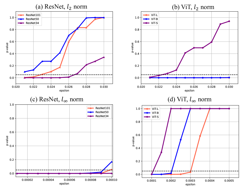
Figure 1: $p$-value vs. attack budget $\epsilon$ for ResNets and ViT’s under AutoAttack with $l_{2}$ norm and $l_{\infty}$ norm. In (b), the curves of ViT-B and ViT-L overlap because they exhibit similar empirical risks.

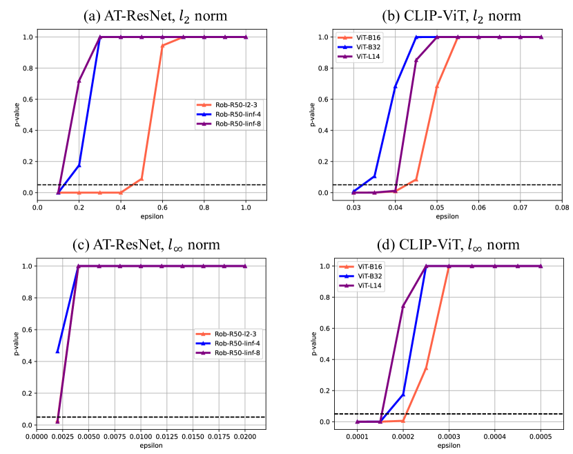
Figure 2: $p$-value vs. attack budget $\epsilon$ for AT Resnets and CLIP-ViT’s under AutoAttack with $l_{2}$ norm and $l_{\infty}$ norm. In (c), the curves of Rob-R50-linf-8 and Rob-R50-l2-3 overlap because they exhibit similar empirical risks.

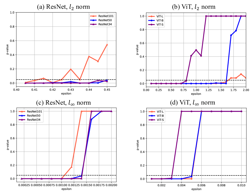
Figure 3: $p$-value vs. attack budget $\epsilon$ for ResNets and ViT’s under SquareAttack with $l_{2}$ norm and $l_{\infty}$ norm.

Figure 4: $p$-value vs. attack budget $\epsilon$ for AT-ResNets and CLIP-ViT’s under SquareAttack with $l_{2}$ norm and $l_{\infty}$ norm. In (c) and (d), the curves of Rob-R50-linf-4 and Rob-R50-linf-8 overlap because they exhibit similar empirical risks.

5 Experiments

We now show how to use PROSAC to certify the performance of various state-of-the-art vision models in the presence of various adversarial attacks; how the framework recovers existing trends relating to the robustness of different models against different adversarial attacks; and how the framework also suggests new trends relating to state-of-the-art model robustness against attacks.

5.1 Experimental Settings

Datasets We will consider primarily classification tasks on the ImageNet-1k dataset [17]. We follow the common experimental setting in black-box adversarial attacks, using 1,000 images from ImageNet-1k [1, 25] to apply our proposed certification procedure. In particular, we take our calibration set to correspond to this dataset.

Models We use two representative state-of-the-art models in computer vision in our experiments, vision transformer (ViT) [18] and ResNet [22]. Three categories of models are used in our experiments. 1) Supervised pre-trained models on ImageNet-1k: We use small, base and large models for both ResNet and ViT. Specifically, we test ViT-Small, ViT-Base and ViT-Large for ViT, and ResNet-34, ResNet-50 and ResNet-101 for ResNet. 2) Self-supervised pre-trained models fine-tuned on ImageNet-1k: We use CLIP models [33] with ViT-B16, ViT-B32 and ViT-L14. 3) Adversarially pre-trained (AT) models on ImageNet-1k: Three ResNet-50 models pre-trained on ImageNet-1k are tested with different attack budgets and $l_{p}$ norms [34] used during adversarial training. Two models use $l_{\infty}$ norm and $\epsilon$=4/255 and 8/255, which we will refer to as Rob-R50-linf-4 and Rob-R50-linf-8, respectively, and one uses $l_{2}$ norm and $\epsilon$=3, which we will refer to as Rob-R50-l2-3. In summary, we test 12 pre-trained models in our experiments.

Adversarial Attacks We use three adversarial attacks in our experiments, including one white-box attack and two black-box attacks. We use AutoAttack [16] to evaluate the white-box adversarial risk, as this is the default benchmark for white-box adversarial robustness in the literature. In the black-box setting, we use SquareAttack [1] and NES attack [25], since both attacks are computationally efficient and effective. Both attacks are score-based; the SquareAttack is considered hyperparameter-free, while the NES attack contains two hyper-parameters, $\lambda_{\sigma}$ and $\lambda_{\eta}$ (see Table 1). We also use both $l_{2}$- and $l_{\infty}$-balls with radius $\epsilon$ to define the various attacks. We set $\alpha=0.10$ and $\zeta=0.05$ in our safety certification procedure, per Definition 1.

5.2 Experimental Results

We now report results relating to the use of PROSAC to certify the performance of the above models in the presence of various attacks, including attacks with fixed and optimizable hyper-parameters.

Adversarial Attacks with Fixed Hyperparameters. Here, we consider SquareAttack and AutoAttack by fixing their hyper-parameters to be equal to the default parameters. It is thus sufficient to certify the machine learning models for different values of the attack budget and different norms. Fig. 1 and 2 depict how the $p$-value behaves as a function of the attack budget for AutoAttack for different machine learning models, with hyper-parameters set equal to the default in [16]. We choose a smaller adversarial attack budget for $l_{\infty}$ constrained attacks as an $l_{2}$ ball of a certain radius is contained by the $l_{\infty}$ ball with the same radius. Fig. 3 and 4 depict how the $p$-value behaves as a function of the attack budget for SquareAttack, where we have set the hyper-parameter corresponding to the probability of changing a particular image pixel to be equal to the default of 0.05 c.f. [1]. Note that different models exhibit radically different behaviours under a SquareAttack, so we also use different attack budget grids for these models. As there are more sources of randomness in SquareAttack than in AutoAttack, we average the empirical risks over 10 trials with different random seeds for a more accurate p-value.

Adversarial Attacks with Free Hyperparameters. We next consider a NES attack where the attacker can choose the two hyper-parameters $\lambda_{\sigma}$ and $\lambda_{\eta}$, shown in Tab. 1, to test the ability of the BO algorithm to certify machine learning model robustness. Bayesian optimization is initialized with 9 initial samples using a two-dimension discrete grid, where $\lambda_{\sigma}=\{\text{0.005, 0.01, 0.015}\}$ and $\lambda_{\eta}=\{\text{0.01, 0.02, 0.03}\}$. During the GP-UCB optimization process, we set $\beta_{\text{UCB}}$=0.1, the interval bound for both hyperparameters $[\text{1e-5},0.1]$ and the number of optimization rounds $T=50$. The supplementary material shows how the number of rounds T in GP-UCB is needed to retain the ($\alpha$,$\zeta$)-safety guarantee. For the attack budget, we use a grid of $\{\text{0.10, 0.15, 0.20, 0.25, 0.30}\}$. We also use a dense grid in Table 2 to show the impact of the grid interval. Tab 2 shows the $p$-value for different $\ell_{2}$-norm constrained attack budgets for the ResNet50 model. Note that we use the GP-UCB as the searching algorithm because of its efficiency in searching for the optimal solution of a black-box function [12].

(a) Sparse Grid

$\epsilon$	0.10	0.15	0.2	0.25	0.3
p-value	0.000	0.009	0.423	1.000	1.000

(b) Dense Grid

$\epsilon$	0.14	0.15	0.16	0.17	0.18
p-value	0.000	0.009	0.029	0.134	0.346

(c) GP-UCB

$\epsilon$	0.14	0.15	0.16	0.17	0.18
p-value	0.000	0.009	0.029	0.134	0.346

Table 2: NES attack with GP-UCB optimization (Alg. 1) for hyperparameter selection with ResNet50 and $l_{2}$ norm.

Discussion. Our experimental results suggest how one can leverage PROSAC to certify the performance of different machine learning models in the presence of different adversarial attacks. In particular, given a specific machine learning model under a specific adversarial attack (with fixed budget and norm), one can leverage the different $p$-value vs. attack budget plots in Figs. 1–4 to establish whether such a model is $(\alpha=0.10,\zeta=0.05)$–safe under such an attack depending on whether the $p$-value is higher or lower than $\zeta=0.05$ (corresponding to the horizontal dashed line in each plot). For example, under a white-box AutoAttack with an $\ell_{2}$-ball with radius $\epsilon=0.026$, one can establish from Fig. 1a that ResNet34 is ($\alpha$=0.10, $\zeta$=0.05)-safe, while ResNet50 and ResNet101 are not; likewise, under the same attack with $\epsilon=0.026$, Fig. 1.b reveals that ViT-S is not ($\alpha$=0.10, $\zeta$=0.05)-safe, while the two larger models are safe.

Moreover, one can leverage the $p$-value vs attack budget plots in Figs. 1–4 to establish a range of attack budgets under which a specific model subject to a specific adversarial attack is $(\alpha=0.10,\zeta=0.05)$-safe. For example, Fig. 1a shows that ResNet34 is $(\alpha=0.10,\zeta=0.05)$-safe under AutoAttack with $l_{2}$ norm provided that the attack budget is smaller than (roughly) 0.027; in turn, Fig. 1b suggests that ViT-S is $(\alpha=0.10,\zeta=0.05)$-safe under AutoAttack with $l_{2}$ norm provided that the attack budget is smaller than (roughly) 0.022. Naturally, we can adopt a similar analysis to establish $(\alpha,\zeta)$-safety guarantees of the other models in the presence of the various attacks under consideration by inspecting Figs. 1–4.

Importantly, our framework leads to results that are consistent with existing results in the literature, thereby further validating our certification procedure. Concretely, beyond showing that different models exhibit different robustness behaviour under different attacks [16], our certification procedure also reveals that:

• The models are less robust to white-box attacks in comparison with black-box attacks. For example, comparing Figs. 1 to 3 or Figs. 2 to 4, it is evident that any of our models appear to be more robust under the SquareAttack than the AutoAttack, since our certification procedure declares them ($\alpha$, $\zeta$)–safe under a wider set of attack budgets.

• The models are less robust to a black-box NES attack, where the attacker can further optimize the attack hyper-parameters, in comparison with a black-box SquareAttack, where the attacker uses a set of fixed hyper-parameters. For example, inspecting Fig. 3 and Table 2, we can declare that ResNet50 is safer under a wider set of attack budgets in the presence of the SquareAttack compared with the NES attack.

• Adversarially trained models are more robust than non-adversarially trained models under different white-box and black-box attacks. Comparing Figs. 1 to 2 or Figs. 3 to 4, it can be seen that adversarially trained ResNets are more robust than standard ResNets, since our procedure declares them to be ($\alpha$, $\zeta$)–safe under a wider set of attack budgets.

• ViTs are generally more adversarially robust than ResNets under both white-box and black-box attacks, corroborating existing observations in [36, 5, 9]. For instance, in Fig. 1-4, ViT-B and ViT-L are certifiably more robust than all ResNets under both attacks.

However, our framework also leads to new observations relating to the robustness of different models to different adversarial attacks that may merit additional investigation. First, the experiments suggest that larger ViT models appear to be more robust than smaller models; in contrast, Resnet model size does not appear to influence its robustness against adversarial attacks much, in line with existing research suggesting that a wider ResNet does not necessarily have stronger adversarial robustness [46]. Second, the experiments suggest that CLIP-ViTs appear to be more vulnerable than supervised trained ViTs under the different attacks, despite the fact that the CLIP models are trained with more data during the self-supervised training stage [33]. This raises questions about the impact of self-supervised training on adversarial robustness or how to harvest the self-supervised learned features in downstream adversarial training.

6 Regulatory Implications

Policy makers and standard setters around the world emphasise the importance of “robust and verifiable measurement methods for risk and trustworthiness” of AI systems, including measures of the resilience of a system against unexpected or adversarial use (or misuse) [40]. For example, the EU AI Act requires systems classified as “high risk” to have risk management systems capable of estimating and evaluating both “the risks that may emerge when the high-risk AI system is used in accordance with its intended purpose and under conditions of reasonably foreseeable misuse” (Art. 9). The Act further stipulates that high risk systems must “achieve an appropriate level of accuracy, robustness and cybersecurity”, including where attempts are made by unauthorised third parties to alter the performance of the system, i.e. where adversarial attacks occur (Art. 15(1), (4)). Levels of accuracy and robustness must be measured and disclosed to users (Art. 15(2)).

While the AI Act requires further implementation and the promulgation of harmonised standards that can be used to assess conformity with the Act (Arts. 40-43), it is clear that the necessary risk assessments (including the risk of an adversarial attack compromising performance) must be made against “preliminarily defined metrics and probabilistic thresholds” (Art. 9(7) AI Act) and take into account “the generally acknowledged state of the art” in engineering and machine learning (AI Act, recital 49 and Art. 9(3)). By providing population-level guarantees that hold for any set of hyperparameters chosen by an attacker and that are based on precise probabilistic thresholds, i.e., ($\alpha$,$\zeta$)-safety, PROSAC offers a state-of-the-art risk assessment tool that is suitable to satisfy the requirements of the AI Act.

Beyond the EU AI Act, PROSAC is also likely to be of relevance as a risk assessment tool. Both the U.S. National Institute of Standards and Technology (NIST) and European standard setting bodies expect firms to analyze, benchmark, and monitor AI risks [40, 31]. According to the NIST AI RMF Playbook, this involves evaluating and documenting the extent to which systems can withstand adverse events (Measure 2.7). PROSAC provides precisely this assessment. Additionally, using state-of-the-art certification procedures and disclosing performance guarantees to operators and end users will typically play a key role in discharging a provider’s duty to act with due care and thus limit liability exposure for negligence.

7 Conclusions

We have proposed PROSAC, a new approach to certify the performance of a machine learning model in the presence of an adversarial attack, with population level adversarial risk guarantees. PROSAC builds on recent work on distribution-free risk quantification approaches, offering an instrument to ascertain whether a model is likely to be safe in the presence of an adversarial attack, independently of how the attacker chooses the attack hyperparameters. We show via experiments that PROSAC is able to certify various state-of-the-art models, leading to results that are in line with existing results in the literature. The technical framework developed here is likely to be of high relevance to AI regulation, such as the EU’s AI Act, which requires providers of certain AI systems to ensure that their systems are resilient to adversarial attacks. Our approach to certifying the performance of any black-box machine learning system offers a tool that can help providers to comply with their legal obligations and show that they acted with due care.

Beyond its utility as a certification instrument, our framework also suggests that a number of areas in adversarial robustness may merit further attention. First, PROSAC has shown that large ViT models appear to be more adversarially robust than smaller models, pointing to new directions for research on the relationship between the capacity of a ViT and its adversarial robustness. Second, CLIP-ViT models appear to be more vulnerable to adversarial attacks than supervised trained ViTs, raising questions about how to use self-supervised models better in improving adversarial robustness of downstream tasks.

Appendix A Proof of Theorem 1

The proof is trivial: We reject / accept the null hypothesis $\mathcal{H}_{0}:\mathcal{R}^{*}>\alpha$ depending on whether or not $p^{*}\leq\zeta$, respectively. The result then follows immediately, because $p^{*}$ is a finite-sample valid $p$-value under the null, i.e. $\mathbb{P}\left(p^{*}\leq\zeta\right)\leq\zeta$ under the null ($0\leq\zeta\leq 1$).

Appendix B Proof of Theorem 2

The proof is also in [26]. In particular, we can establish that

$$\mathbb{P}\left(p^{*}\leq\zeta\right)=\mathbb{P}\left(\max_{\lambda\in\Lambda}p(\lambda)\leq\zeta\right)=\mathbb{P}\left(p\leq\zeta,\forall~{}\lambda\in\Lambda\right)\leq\max_{\lambda\in\Lambda}\mathbb{P}\left(p(\lambda)\leq\zeta\right)\leq\zeta$$ (14)

where the last step follows from the fact that $\mathbb{P}\left(p(\lambda)\leq\zeta\right)\leq\zeta,\forall~{}\lambda\in\Lambda$. Therefore, $p^{*}=\max_{\lambda\in\Lambda}p(\lambda)$ is a (super-uniform) p-value associated with the null hypothesis $\mathcal{H}_{0}:\exists~{}\lambda,\mathcal{R}(\lambda)>\alpha$.

Appendix C Proof of Theorem 3

The proof follows immediately from [4] with some minor modifications that accommodate for the fact that the attack can be stochastic.

Fix the attacker hyper-parameter configuration $\lambda\in\Lambda$. We can show based on the tighter version of Hoeffding’s inequality [24] that for any $\mathcal{R}(\lambda)>\alpha$ it holds

$$\mathbb{P}\left(\hat{\mathcal{R}}(\lambda)\leq\alpha\right)\leq\exp\left(-n\cdot h_{1}\left(\alpha;\mathcal{R}(\lambda)\right)\right)$$ (15)

We can also show based on Bentkus inequality that it holds

$$\mathbb{P}\left(\hat{\mathcal{R}}(\lambda)\leq\alpha\right)\leq e\cdot\mathbb{P}\left({\sf Bin}(n,\mathcal{R}(\lambda))\leq\left\lceil n\cdot\alpha\right\rceil\right)$$ (16)

Therefore, via the hybridization of the Hoeffding and Bentkus inequalities [4] it also follows that

$$\mathbb{P}\left(\hat{\mathcal{R}}(\lambda)\leq\alpha\right)\leq\min\left\{\exp\left(-n\cdot h_{1}\left(\alpha;\mathcal{R}(\lambda)\right)\right),e\cdot\mathbb{P}\left({\sf Bin}(n,\mathcal{R}(\lambda))\leq\left\lceil n\cdot\alpha\right\rceil\right)\right\}$$ (17)

implying that [4]

$$p(\lambda)=\min\left\{\exp\left(-n\cdot h_{1}\left(\hat{\mathcal{R}}(\lambda)\wedge\alpha,\alpha\right)\right),e\cdot\mathbb{P}\left({\sf Bin}(n,\alpha)\leq\left\lceil n\cdot\hat{\mathcal{R}}(\lambda)\right\rceil\right)\right\}$$ (18)

is a valid $p$-value associated with the null hypothesis $\mathcal{H}_{0}:\mathcal{R}(\lambda)>\alpha$ and – via Theorem 3

$$p^{*}=\max_{\lambda\in\Lambda}\min\left\{\exp\left(-n\cdot h_{1}\left(\hat{\mathcal{R}}(\lambda)\wedge\alpha,\alpha\right)\right),e\cdot\mathbb{P}\left({\sf Bin}(n,\alpha)\leq\left\lceil n\cdot\hat{\mathcal{R}}(\lambda)\right\rceil\right)\right\}$$ (19)

is a valid $p$-value associated with the null hypothesis $\mathcal{H}_{0}:\exists\lambda:\mathcal{R}(\lambda)>\alpha$.

Appendix D Proof of Theorem 4

The proof builds on a classical result establishing regret bounds for Gaussian Process Upper Confidence Bound (GP-UCB) optimization from [12]. It is assumed that the p-value lies in an RKHS $\mathcal{H}_{k}$ with some known kernel $k$, such that $\|p\|_{k}\leq B$, and that the noise sequence is conditionally $R$-sub-Gaussian, as in [12].

Let $\hat{p}_{t}$ correspond to the $p$-value evaluation corresponding to the GP-UCB’s decision $\lambda_{t}$ at round $t$, i.e., $\hat{p}_{t}=p(\lambda_{t})$. We let $\hat{p}_{T}=1/T\sum_{t=1}^{T}\hat{p}_{t}$ correspond to the GP-UCB algorithm (maximal) $p$-value approximation (after $T$ rounds) and $p^{*}$ correspond to the exact (maximal) $p$-value appearing in Theorem 3. We can establish from [12] that with probability at least $1-\delta$ (with $\delta\in(0,1)$)

$$p^{*}-\hat{p}_{T}\leq\mathcal{O}\left(B\sqrt{\gamma_{T}/T}+\sqrt{\gamma_{T}\left(\gamma_{T}+\log(1/\delta)\right)/T}\right),$$ (20)

where $\gamma_{T}$ corresponds to the maximum information gain at round $T$ [12]. We can also establish that

$$\hat{p}_{T}\geq p^{*}-\mathcal{O}\left(B\sqrt{\gamma_{T}/T}+\sqrt{\gamma_{T}\left(\gamma_{T}+\log(1/\delta)\right)/T}\right)$$ (21)

with probability greater than $1-\delta$, and

$$\hat{p}_{T}<p^{*}-\mathcal{O}\left(B\sqrt{\gamma_{T}/T}+\sqrt{\gamma_{T}\left(\gamma_{T}+\log(1/\delta)\right)/T}\right)$$ (22)

with probability less than $\delta$.

We now propose to reject or accept the hypothesis $\mathcal{H}_{0}:\mathcal{R}^{*}>\alpha$ by comparing $\hat{p}_{T}$ to a threshold $\zeta^{\prime}$ in lieu of the original threshold $\zeta$, where we will define the value of the new threshold later, because we can only guarantee that $\hat{p}_{T}$ is close to $p^{*}$ – per equation 20 – with probability $1-\delta$.

We next quantify the probability of rejecting the null hypothesis given the null hypothesis is true. In particular, as per the law of total probability, we can show that

$$\mathbb{P}\left(\hat{p}_{T}\leq\zeta^{\prime}\right) =\mathbb{P}\Big{(}\hat{p}_{T}\leq\zeta^{\prime}~{}\big{|}~{}\hat{p}_{T}\geq p^{*}-\mathcal{O}\left(B\sqrt{\gamma_{T}/T}+\sqrt{\gamma_{T}\left(\gamma_{T}+\log(1/\delta)\right)/T}\right)\Big{)}\times$$

$$\qquad\qquad\times\mathbb{P}\left(\hat{p}_{T}\geq p^{*}-\mathcal{O}\left(B\sqrt{\gamma_{T}/T}+\sqrt{\gamma_{T}\left(\gamma_{T}+\log(1/\delta)\right)/T}\right)\right)+$$

$$=\mathbb{P}\Big{(}\hat{p}_{T}\leq\zeta^{\prime}~{}\big{|}~{}\hat{p}_{T}<p^{*}-\mathcal{O}\left(B\sqrt{\gamma_{T}/T}+\sqrt{\gamma_{T}\left(\gamma_{T}+\log(1/\delta)\right)/T}\right)\Big{)}\times$$

$$\qquad\qquad\times\mathbb{P}\left(\hat{p}_{T}<p^{*}-\mathcal{O}\left(B\sqrt{\gamma_{T}/T}+\sqrt{\gamma_{T}\left(\gamma_{T}+\log(1/\delta)\right)/T}\right)\right)$$ (23)

We upper bound the first probability in equation 23 as follows:

$$\mathbb{P}\Big{(}\hat{p}_{T}\leq\zeta^{\prime}~{}\big{|}~{}\hat{p}_{T}\geq p^{*}-\mathcal{O}\left(B\sqrt{\gamma_{T}/T}+\sqrt{\gamma_{T}\left(\gamma_{T}+\log(1/\delta)\right)/T}\right)\Big{)}\leq$$

$$\leq\mathbb{P}\left(p^{*}\leq\zeta^{\prime}+\mathcal{O}\left(B\sqrt{\gamma_{T}/T}+\sqrt{\gamma_{T}\left(\gamma_{T}+\log(1/\delta)\right)/T}\right)\right)\leq$$

$$\leq\zeta^{\prime}+\mathcal{O}\left(B\sqrt{\gamma_{T}/T}+\sqrt{\gamma_{T}\left(\gamma_{T}+\log(1/\delta)\right)/T}\right)$$ (24)

because $\hat{p}_{T}\leq\zeta^{\prime}\implies p^{*}\leq\zeta^{\prime}+\mathcal{O}\left(B\sqrt{\gamma_{T}/T}+\sqrt{\gamma_{T}\left(\gamma_{T}+\log(1/\delta)\right)/T}\right)$ under the condition $\hat{p}_{T}\leq p^{*}-\mathcal{O}\left(B\sqrt{\gamma_{T}/T}+\sqrt{\gamma_{T}\left(\gamma_{T}+\log(1/\delta)\right)/T}\right)$.

We trivially upper bound the third probability in equation 23 as follows:

$$\mathbb{P}\Big{(}\hat{p}_{T}\leq\zeta^{\prime}~{}\big{|}~{}\hat{p}_{T}<p^{*}-\mathcal{O}\left(B\sqrt{\gamma_{T}/T}+\sqrt{\gamma_{T}\left(\gamma_{T}+\log(1/\delta)\right)/T}\right)\Big{)}\leq 1$$ (25)

Furthermore, in view of the probabilistic guarantee associated with the GP UCB algorithm in equation 20, we also upper bound the remaining probabilities as follows:

$$\mathbb{P}\left(\hat{p}_{T}<p^{*}-\mathcal{O}\left(B\sqrt{\gamma_{T}/T}+\sqrt{\gamma_{T}\left(\gamma_{T}+\log(1/\delta)\right)/T}\right)\right)\leq 1$$ (26)

and

$$\mathbb{P}\left(\hat{p}_{T}\geq p^{*}-\mathcal{O}\left(B\sqrt{\gamma_{T}/T}+\sqrt{\gamma_{T}\left(\gamma_{T}+\log(1/\delta)\right)/T}\right)\right)\leq\delta$$ (27)

Putting this together, it follows that – under the null hypothesis – we have

$$\mathbb{P}\left(\hat{p}_{T}\leq\zeta^{\prime}\right)\leq\zeta^{\prime}+\mathcal{O}\left(B\sqrt{\gamma_{T}/T}+\sqrt{\gamma_{T}\left(\gamma_{T}+\log(1/\delta)\right)/T}\right)+\delta$$ (28)

Finally, we guarantee $(\alpha,\zeta)$ model safety by choosing a new threshold $\zeta^{\prime}=\zeta-\mathcal{O}\left(B\sqrt{\gamma_{T}/T}+\sqrt{\gamma_{T}\left(\gamma_{T}+\log(1/\delta)\right)/T}\right)-\delta$. Note we can guarantee $\zeta>\mathcal{O}\left(B\sqrt{\gamma_{T}/T}+\sqrt{\gamma_{T}\left(\gamma_{T}+\log(1/\delta)\right)/T}\right)+\delta$ by choosing the number of GP UCB rounds to be sufficiently large, for any $\delta<\zeta$.

References

- [1] Maksym Andriushchenko, Francesco Croce, Nicolas Flammarion and Matthias Hein “Square attack: a query-efficient black-box adversarial attack via random search” In European conference on computer vision, 2020, pp. 484–501 Springer
- [2] Anastasios Angelopoulos and Stephen Bates “Conformal Prediction: A Gentle Introduction” In Foundations and Trends in Machine Learning 31, 2023
- [3] Anastasios N Angelopoulos et al. “Learn then test: Calibrating predictive algorithms to achieve risk control” In arXiv preprint arXiv:2110.01052, 2021
- [4] Stephen Bates et al. “Distribution-free, risk-controlling prediction sets” In Journal of the ACM (JACM) 68.6 ACM New York, NY, 2021, pp. 1–34
- [5] Srinadh Bhojanapalli et al. “Understanding robustness of transformers for image classification” In Proceedings of the IEEE/CVF international conference on computer vision, 2021, pp. 10231–10241
- [6] Emily Black, Samuel Yeom and Matt Fredrikson “Fliptest: fairness testing via optimal transport” In Proceedings of the 2020 Conference on Fairness, Accountability, and Transparency, 2020, pp. 111–121
- [7] Joan Bruna et al. “Intriguing properties of neural networks” In International Conference on Learning Representations, 2014
- [8] Nicholas Carlini and David Wagner “Towards evaluating the robustness of neural networks” In 2017 ieee symposium on security and privacy (sp), 2017, pp. 39–57 Ieee
- [9] Nicholas Carlini et al. “(Certified!!) Adversarial Robustness for Free!” In The Eleventh International Conference on Learning Representations, 2023 URL: https://openreview.net/forum?id=JLg5aHHv7j
- [10] Anirban Chakraborty et al. “Adversarial Attacks and Defences: A Survey” In arXiv:1810.00069, 2018
- [11] Jianbo Chen, Michael I Jordan and Martin J Wainwright “Hopskipjumpattack: A query-efficient decision-based attack” In 2020 ieee symposium on security and privacy (sp), 2020, pp. 1277–1294 IEEE
- [12] Sayak Ray Chowdhury and Aditya Gopalan “On kernelized multi-armed bandits” In International Conference on Machine Learning, 2017, pp. 844–853 PMLR
- [13] Ben Chugg, Santiago Cortes-Gomez, Bryan Wilder and Aaditya Ramdas “Auditing Fairness by Betting” In arXiv preprint arXiv:2305.17570, 2023
- [14] Jeremy Cohen, Elan Rosenfeld and Zico Kolter “Certified adversarial robustness via randomized smoothing” In international conference on machine learning, 2019, pp. 1310–1320 PMLR
- [15] Francesco Croce and Matthias Hein “Minimally distorted adversarial examples with a fast adaptive boundary attack” In International Conference on Machine Learning, 2020, pp. 2196–2205 PMLR
- [16] Francesco Croce and Matthias Hein “Reliable evaluation of adversarial robustness with an ensemble of diverse parameter-free attacks” In International conference on machine learning, 2020, pp. 2206–2216 PMLR
- [17] Jia Deng et al. “Imagenet: A large-scale hierarchical image database” In 2009 IEEE conference on computer vision and pattern recognition, 2009, pp. 248–255 Ieee
- [18] Alexey Dosovitskiy et al. “An Image is Worth 16x16 Words: Transformers for Image Recognition at Scale” In International Conference on Learning Representations, 2020
- [19] Marc G Genton “Classes of kernels for machine learning: a statistics perspective” In Journal of machine learning research 2.Dec, 2001, pp. 299–312
- [20] Sven Gowal et al. “On the effectiveness of interval bound propagation for training verifiably robust models” In arXiv preprint arXiv:1810.12715, 2018
- [21] Sven Gowal et al. “Scalable verified training for provably robust image classification” In Proceedings of the IEEE/CVF International Conference on Computer Vision, 2019, pp. 4842–4851
- [22] Kaiming He, Xiangyu Zhang, Shaoqing Ren and Jian Sun “Deep residual learning for image recognition” In Proceedings of the IEEE conference on computer vision and pattern recognition, 2016, pp. 770–778
- [23] Matthias Hein and Maksym Andriushchenko “Formal guarantees on the robustness of a classifier against adversarial manipulation” In Advances in neural information processing systems 30, 2017
- [24] Wassily Hoeffding “Probability inequalities for sums of bounded random variables” In The collected works of Wassily Hoeffding Springer, 1994, pp. 409–426
- [25] Andrew Ilyas, Logan Engstrom, Anish Athalye and Jessy Lin “Black-box adversarial attacks with limited queries and information” In International conference on machine learning, 2018, pp. 2137–2146 PMLR
- [26] Bracha Laufer-Goldshtein, Adam Fisch, Regina Barzilay and Tommi Jaakkola “Efficiently controlling multiple risks with Pareto testing” In International Conference on Learning Representations, 2023
- [27] Mathias Lecuyer et al. “Certified robustness to adversarial examples with differential privacy” In 2019 IEEE symposium on security and privacy (SP), 2019, pp. 656–672 IEEE
- [28] Klas Leino, Zifan Wang and Matt Fredrikson “Globally-robust neural networks” In International Conference on Machine Learning, 2021, pp. 6212–6222 PMLR
- [29] Linyi Li, Tao Xie and Bo Li “Sok: Certified robustness for deep neural networks” In 2023 IEEE Symposium on Security and Privacy (SP), 2023, pp. 1289–1310 IEEE
- [30] Aleksander Madry et al. “Towards Deep Learning Models Resistant to Adversarial Attacks” In International Conference on Learning Representations, 2018
- [31] Supreme Audit Institutions Netherlands Norway and UK “Auditing machine learning algorithms: A white paper for public auditors”, 2023
- [32] Victor Quach et al. “Conformal Language Modeling” In arXiv preprint arXiv:2306.10193, 2023
- [33] Alec Radford et al. “Learning transferable visual models from natural language supervision” In International conference on machine learning, 2021, pp. 8748–8763 PMLR
- [34] Hadi Salman et al. “Do adversarially robust imagenet models transfer better?” In Advances in Neural Information Processing Systems 33, 2020, pp. 3533–3545
- [35] Hadi Salman et al. “Provably robust deep learning via adversarially trained smoothed classifiers” In Advances in Neural Information Processing Systems 32, 2019
- [36] Rulin Shao et al. “On the Adversarial Robustness of Vision Transformers” In Transactions on Machine Learning Research, 2022
- [37] Nian Si, Karthyek Murthy, Jose Blanchet and Viet Anh Nguyen “Testing group fairness via optimal transport projections” In International Conference on Machine Learning, 2021, pp. 9649–9659 PMLR
- [38] Sahil Singla and Soheil Feizi “Skew orthogonal convolutions” In International Conference on Machine Learning, 2021, pp. 9756–9766 PMLR
- [39] Niranjan Srinivas, Andreas Krause, Sham Kakade and Matthias Seeger “Gaussian process optimization in the bandit setting: no regret and experimental design” In Proceedings of the 27th International Conference on International Conference on Machine Learning, 2010, pp. 1015–1022
- [40] National Institute Standards and Technology (NIST) “Artificial Intelligence Risk Management Framework (AI RMF 1.0)”, 2023
- [41] Bahar Taskesen, Jose Blanchet, Daniel Kuhn and Viet Anh Nguyen “A statistical test for probabilistic fairness” In Proceedings of the 2021 ACM Conference on Fairness, Accountability, and Transparency, 2021, pp. 648–665
- [42] Asher Trockman and J Zico Kolter “Orthogonalizing Convolutional Layers with the Cayley Transform” In International Conference on Learning Representations, 2020
- [43] Yusuke Tsuzuku, Issei Sato and Masashi Sugiyama “Lipschitz-margin training: Scalable certification of perturbation invariance for deep neural networks” In Advances in neural information processing systems 31, 2018
- [44] Eric Wong and Zico Kolter “Provable defenses against adversarial examples via the convex outer adversarial polytope” In International conference on machine learning, 2018, pp. 5286–5295 PMLR
- [45] Eric Wong, Frank Schmidt, Jan Hendrik Metzen and J Zico Kolter “Scaling provable adversarial defenses” In Advances in Neural Information Processing Systems 31, 2018
- [46] Boxi Wu et al. “Do wider neural networks really help adversarial robustness?” In Advances in Neural Information Processing Systems 34, 2021, pp. 7054–7067
- [47] Xiaojun Xu, Linyi Li and Bo Li “Lot: Layer-wise orthogonal training on improving l2 certified robustness” In Advances in Neural Information Processing Systems 35, 2022, pp. 18904–18915
- [48] Songkai Xue, Mikhail Yurochkin and Yuekai Sun “Auditing ml models for individual bias and unfairness” In International Conference on Artificial Intelligence and Statistics, 2020, pp. 4552–4562 PMLR
- [49] Bohang Zhang, Du Jiang, Di He and Liwei Wang “Boosting the Certified Robustness of L-infinity Distance Nets” In International Conference on Learning Representations, 2021
- [50] Huan Zhang et al. “Towards Stable and Efficient Training of Verifiably Robust Neural Networks” In International Conference on Learning Representations, 2019