Abstract

Language Models (LMs) are increasingly used for a wide range of prediction tasks, but their training can often neglect rare edge cases, reducing their reliability. Here, we define a stringent standard of trustworthiness whereby the task algorithm and circuit implementation must be verified, accounting for edge cases, with no known failure modes. We show that a transformer model can be trained to meet this standard if built using mathematically and logically specified frameworks. In this paper, we fully verify a model for n-digit integer addition. To exhibit the reusability of verified modules, we insert the trained integer addition model into an untrained model and train the combined model to perform both addition and subtraction. We find extensive reuse of the addition circuits for both tasks, easing verification of the more complex subtractor model. We discuss how inserting verified task modules into LMs can leverage model reuse to improve verifiability and trustworthiness of language models built using them. The reuse of verified circuits reduces the effort to verify more complex composite models which we believe to be a significant step towards safety of language models.

1 Introduction

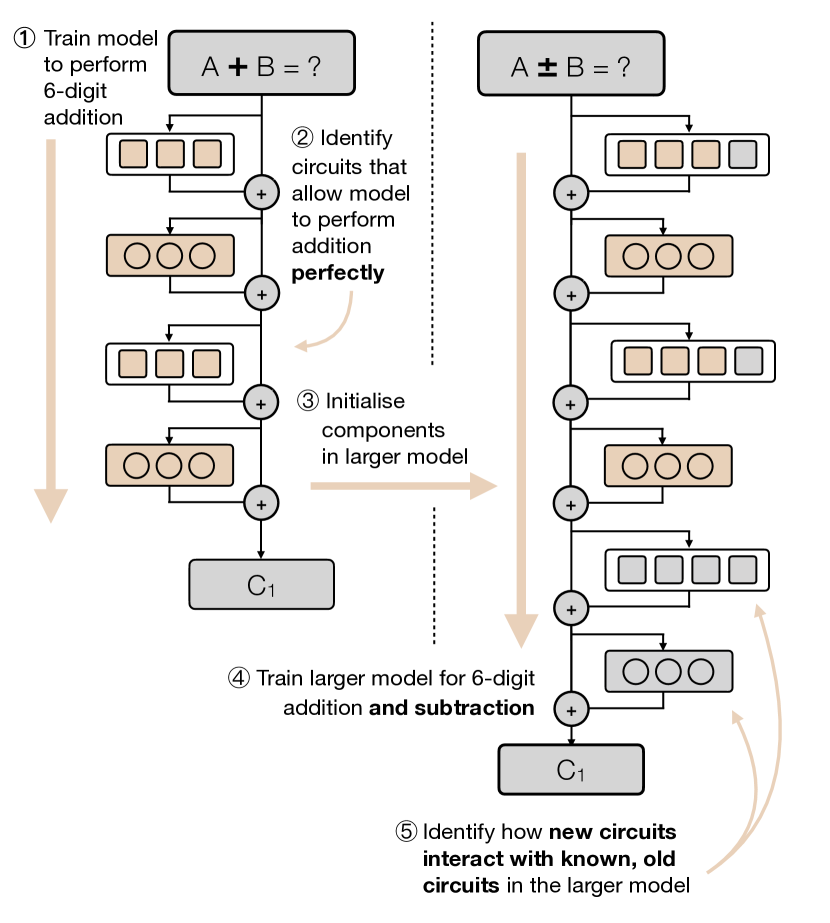
Figure 1: An overview of our methodology: (1) We trained a perfectly accurate 6-digit integer addition model. (2) We reverse-engineered the model to find the algorithms that were implemented to perform addition. (3) We inserted the addition model into a new model, by copying the weights of the attention heads and MLPs (in brown) into the larger model during initialisation. (4) We then train the new model on 80% subtraction and 20% addition questions. (5) We find that the resulting model reuses the inserted addition circuits for both addition and subtraction questions.

Transformer-based large language models (LLMs) are powerful (Barak et al., 2022) yet largely inscrutable due to their complex, nonlinear interactions in dense layers within high-dimensional spaces. Given this complexity, their deployment in critical settings (Zhang et al., 2022) highlights the need for understanding their behavior. Many argue that making these models interpretable is key to their safe use (Hendrycks & Mazeika, 2022).

Mechanistic interpretability focuses on demystifying and validating the algorithms behind model weights, translating complex computations into more human-understandable components (Raukur et al., 2022). This understanding aids in predicting model behavior in new situations and fixing model errors.

In creating and training a model, we would ideally want the model to have a very high standard of accuracy and trustworthiness. We aim to achieve this by holding the model to a standard that we term known-good. A model performing a task is known-good if:

1. The model’s algorithm for the task and the mechanisms it implements (the “circuits”) are understood.

2. All possible edge cases have been identified and tested. As a heuristic, the model should be able to perform the task one million times without error (“1M Q accuracy”).

3. The model has no known failure modes.

However, exhaustive testing of a model for most tasks is unfeasible. For instance, a task involving the addition of 5-digit integers (e.g., 12345+67890) presents ten billion possible variations. Rather than testing every variation, the task can be conceptualized within a formal framework to pinpoint edge cases the model must handle. For example, in 5-digit addition, the most uncommon edge case is 55555+44445=100000, which requires a carry bit to cascade through all digits, occurring in only 0.002% of cases. A known-good model must incorporate algorithms to manage this and other more frequent edge cases. A known-good model would hence have circuits that are verified to perform the task perfectly.

In this paper, we detail the development and interpretation of a known-good model for addition. Our findings indicate that the model constructs a specific circuit for each edge case, with these circuits sharing intermediate results. We confirm the validity of the entire set of circuits, ensuring they cover all identified edge cases. The model achieves a very low training loss and can do one million predictions without error, making it a known-good model.

Additionally, we develop a “mixed” model capable of both addition and subtraction, incorporating the known-good addition model. This mixed model extensively reuses the addition circuits for both operations and learns new circuits, facilitating the interpretation of the model’s algorithm. This approach marks progress toward a known-good model for both addition and subtraction.

Hence, our main contributions are three-fold:

• A trustworthy known-good 5-digit addition model, with an algorithm extensible to n-digits.

• A 6-digit addition and subtraction model that reuses established addition circuits for both operations, indicating steps toward a known-good model for these tasks.

• A proof of concept for enhancing the trustworthiness of a larger model by integrating a smaller known-good transformer model.

2 Related Work

Mechanistic interpretability aims to reverse engineer neural networks to find interpretable algorithms that are implemented in a model’s weights (Olah et al., 2020). To better represent these algorithms, Elhage et al. (2021a) introduced a mathematical framework to represent how transformer attention heads can work with each other to implement complex algorithms.

To explain how (not where) a model algorithm is implemented, Jenner et al. (2023) recommends documenting a low-level computation graph (causal abstraction), with a mapping from the graph to the model nodes that implement the computation, with experimentation verification.

Investigative techniques such as ablation interventions, activation unembeddings (nostalgebraist, 2020), and sparse autoencoders (Nanda, 2023; Cunningham et al., 2023), underpinned by the more theoretical frameworks (Elhage et al., 2021b; Geva et al., 2022), provide tools to help confirm a mapping.

Investigating pre-trained LMs on Arithmetic. Even though basic arithmetic can be solved following a few simple rules, pre-trained LMs often struggle to solve simple math questions (Hendrycks et al., 2021). Stolfo et al. (2023) used causal mediation analysis to investigate how large pre-trained LMs like Pythia and GPT-J performed addition to solve word problems.

It is also possible to improve a model’s arithmetic abilities through training data enrichment. Liu & Low (2023) used supervised fine tuning (including enriched training data) to convert LLaMA 7B to Goat - a model that is “Good at Arithmetic Tasks” including addition and subtraction. They also showed the model’s performance relied in part on LLaMA’s consistent tokenization of digits.

Studying Toy Models for Arithmetic. Doing mechanistic interpretability on toy transformers can help to better isolate clear, distinct circuits given the highly specific experimental setup for the model studied. Nanda et al. (2023) studied modular addition in a one-layer transformer (where each number was represented by a distinct token) to better understand training dynamics.

Quirke & Barez (2024) detailed how a 1-layer, 3-head transformer model performed 5-digit addition questions. It showed a rare edge case (e.g. “77778+22222=100000” where a “carry 1” cascades through 4 digits) that the model couldn’t handle - showing the importance of understanding and testing all edge cases for trustworthiness.

Michaud et al. (2023) posits that many natural prediction problems decompose into a finite set of knowledge and skills that are “quantized” into discrete chunks (quanta). Models must learn these quanta to reduce loss. They posit that “understanding a network reduces to enumerating its quanta.” Schaeffer et al. (2023) provides useful ways to measure quanta in mathematical prediction problems.

3 Methodology

3.1 Mathematical Framework

Consider the task of adding two $n$-digit numbers together. Let us define the first number as $D=\{D_{n-1},D_{n-2},\ldots,D_{0}\}$ and the second number as $D^{\prime}=\{D^{\prime}_{n-1},D^{\prime}_{n-2},\ldots,D^{\prime}_{0}\}$. The resulting answer can be represented as $A=\{A_{n},A_{n-1},\ldots,A_{0}\}$. For an illustrative example, see Figure 2.

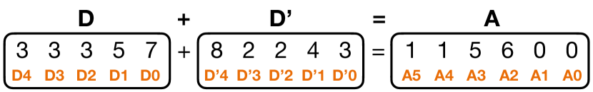
Figure 2: We refer to individual tokens in a 5-digit addition question as D4, .. D0, and D’4, .., D’0 and the answer tokens as A5, .., A0. For n-digits, we use the terms $D_{n}$, $D^{\prime}_{n}$and $A_{n}$.

We categorize the sum of each digit pair into three overlapping groups BA, MC and US defined as:

$$BA_{n}=(D_{n}+D^{\prime}_{n})\mod 10$$ (1)

$$MC_{n}=\begin{cases}1&\text{if }(D_{n}+D^{\prime}_{n})\geq 10,\\ 0&\text{otherwise}.\end{cases}$$ (2)

$$US_{n}=\begin{cases}1&\text{if }(D_{n}+D^{\prime}_{n})=9,\\ 0&\text{otherwise}.\end{cases}$$ (3)

When calculating $(A_{n})$, considering only the carry bit from the two preceding digits, we have:

$$A_{n}=\begin{cases}D_{n}+D^{\prime}_{n}+1\underbrace{\text{mod}}_{10},&\text{if }\underbrace{MC}_{n-1}=1\text{ or}\\ &(\underbrace{US}_{n-1}=1\text{ and }\underbrace{MC}_{n-2}=1),\\ D_{n}+D^{\prime}_{n}\underbrace{\text{mod}}_{10},&\text{otherwise.}\end{cases}$$ (4)

This approach is aligned with the framework implemented by the addition model in Quirke & Barez (2024). However, it is restricted to cases where the carry bit cascades over two or fewer digits. To address this limitation, we introduce an additional digit-level categorization called TriCase:

$$D_{n}.C=\underbrace{\text{TriCase}}_{(D_{n},D^{\prime}_{n})}=\begin{cases}T10&\text{if }(D_{n}+D^{\prime}_{n})\geq 10,\\ T9&\text{if }(D_{n}+D^{\prime}_{n})=9,\\ T8&\text{if }(D_{n}+D^{\prime}_{n})\leq 8.\end{cases}$$ (5)

These categorization cases contain carry bit information:

• If $D_{n}.C=T10$, the digit-pair always causes a MC,

• if $D_{n}.C=T9$, the digit-pair will cause an MC if the proceeding digit-pair sum generates an MC, and

• if $D_{n}.C=T8$, the digit-pair never causes an MC .

To compute the first digit of the answer in a problem such as $(55555+44445=)$, the algorithm must synthesize the five TriCase values from the respective digit-pairs. This synthesis is crucial to determine the presence of a carry bit cascading through all five digits.

We introduce a function, TriAdd, to facilitate the transfer of TriCase data between digits. It is defined as follows:

$$\underbrace{\text{TriAdd}}_{(D_{n}.C,D_{n-1}.C)}=\begin{cases}T10&\text{if }D_{n}.C=T10\\ &\text{or }D_{n}.C=T9\\ &\text{\quad and }D_{n-1}.C=T10,\\ T9&\text{if }D_{n}.C=T8\\ &\text{\quad and }D_{n-1}.C=T10,\\ T8&\text{otherwise.}\end{cases}$$ (6)

TriAdd transfers MC data from $(D_{n-1})$ to $(D_{n})$ by integrating the values of $(D_{n}.C)$ and $(D_{n-1}.C)$. This function can be represented as nine bigram mappings and yields three distinct outputs (details in App. D). Finally, we introduce the recursive function $D_{n}$.$C_{m}$ , which aggregates TriCase data across $(m)$ digits to enhance accuracy.

$$D_{n}.C_{m}=\begin{cases}\underbrace{\text{TriAdd}}_{(D_{n}.C,D_{n-1}.C_{m-1})}&\text{if }m>2,\\ \underbrace{\text{TriAdd}}_{(D_{n}.C,D_{n-1}.C)}&\text{if }m=2.\end{cases}$$ (7)

Simply put $D_{n}$.$C_{m}$ cascades the carry bit over $m$ digits. Calculating $D_{1}.C_{2}$ means calculating $\text{TriAdd}(D_{1}.C,D_{0}.C)$ combining the $D_{0}$-specific TriCase value and $D_{1}$-specific TriCase value to give a perfectly accurate TriCase value for $D_{1}$. Calculating $D_{4}.C_{5}$ means calculating $\text{TriAdd}(D_{4}.C,D_{3}.C_{4})$ combining the $D_{4}$-specific TriCase value with the perfectly accurate $D_{3}.C_{4}$ TriCase value to give a perfectly accurate TriCase value for $D_{4}$.

In 5-digit addition, the values D4.C5, D3.C4, D2.C3 and D1.C2 are perfectly accurate as they integrate TriCase data all the way back to and including D0.MC . An accurate algorithm must calculate these values. Works on 5-digit model was unable to calculate these $D_{n}$.$C_{m}$ and so was not perfectly accurate (Quirke & Barez, 2024) . As shown later, our model’s algorithm incorporates the (Quirke & Barez, 2024) algorithm, and adds these perfectly accurate $D_{n}$.$C_{m}$ . Figure 3 shows the combined algorithm.

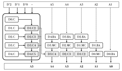
Figure 3: In 5-digit addition the model first calculates all $D_{n}.C$ values, then combines them into perfectly accurate $D_{n}$.$C_{m}$ values by P11 (token =) when A5 is predicted. From P12, the remaining answer digits are calculated one by one, using $D_{n}$.$C_{m}$ values if needed. This algorithm can be extended to generalise to n-digits.

3.2 Question Difficulty and Frequency

To analyse question difficulty, we categorised questions by the complexity of the computation required to solve the question, as shown in Tab. 1. The categories are arranged according to the number of digits that a carry bit has to cascade through.

Table 1: We categorise addition questions into non-overlapping “calculation complexity” quanta, ordered by increased computational difficulty (and decreasing occurrence frequency). Five-digit addition questions quanta are S0 to S5. Ten-digit addition question quanta are S0 to S10. S10’s frequency is $\sim 3\times 10^{-4}$ showing the need to enrich training data for rare edge cases.

Name	Contains	Example	Freq
S0	BA	11111+12345=23456	$\sim$5%
S1	BA,MC	11111+9=22230	$\sim$21%
S2	BA,MC,US	11111+89=22300	$\sim$34%
S3	BA,MC,USx2	11111+889=23000	$\sim$28%
S4	BA,MC,USx3	11111+8889=30000	$\sim$11%
S5	BA,MC,USx4	11111+88889=100000	$\sim$2%

3.3 Techniques

In investigating the circuits of the model, we want to understand what each attention head or MLP layer is doing across each token position, and how it relates to our mathematical framework. Hence, we define a node as the computation done by an attention head or MLP layer for a given token position.

Mean ablation. To find out how the model depends on the output of a node, we replace the output of that node with the vector that is the mean of all of its outputs across its batch.

Attention Patterns. To find out what the model attends to at that node, we take the attention pattern at that token position and take the significant tokens attended to ($>0.01$ post softmax).

4 Experiments

4.1 Training & Investigating Five-Digit Addition Model

Training the model. The 5-digit 1-layer addition model in Quirke & Barez (2024) achieved an accuracy of approximately 99%. Our preliminary experiments indicated that a 2-layer, 3-head model was the smallest configuration capable of achieving fully accurate addition (see App. C for alternative configurations tested).

This configuration effectively doubled the computational power compared to the 1-layer model. Moreover, a 2-layer model introduces the capability to “compose” the attention heads in novel ways, facilitating the implementation of more complex algorithms (Elhage et al., 2021b).

By enriching the training dataset with more instances of rare edge cases and using 30 thousand training batches, the 5-digit 2-layer model attained a final training loss of approximately $2.3\times 10^{-8}$. This model demonstrated a 1M Q accuracy (details in App. B).

Investigating the model. To gain insights into the model’s predictive behavior, we conducted an investigation focusing on its activity during prediction calculations. Ablation experiments targeting the nodes revealed that the model primarily depends on nodes located in token positions D’2 to A1, as illustrated in Figs 4 and 5. Across these nine positions, the model engages 36 nodes, comprising 21 attention head nodes and 15 MLP layer nodes. The effects of node ablation on our complexity and answer-impact metrics were analyzed (see Figs 6 and 7), elucidating the specific computations performed at each node.

For each answer digit $A_{n}$using test questions corresponding to the T8, T9 and T10 categories, we performed Principal Component Analysis (PCA) on the nodes yielding interpretable results. Specifically nine “node and answer-digit” combinations (see Figs 13 and 14) showed strong clustering of the questions aligned to the T8, T9 and T10 categories, suggesting these nodes are implementing the TriCase categorisation.

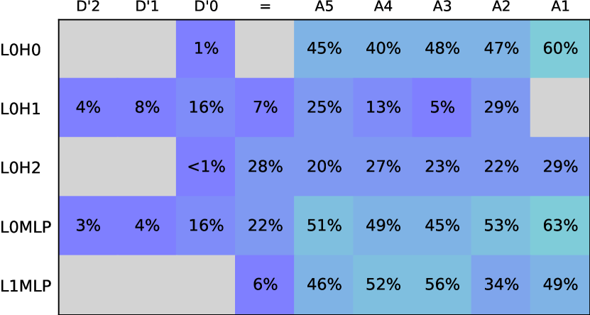
Figure 4: This map shows the % of enriched questions that fail when we ablate each node in the 5-digit 2-layer 3-head addition model. The model only uses nodes in token positions P8 to P16 (tokens D’2 to A1). No attention heads in layer 1 are used. Lower percentages correspond to rarer edge cases. The grey space represents nodes that are not used by the model.

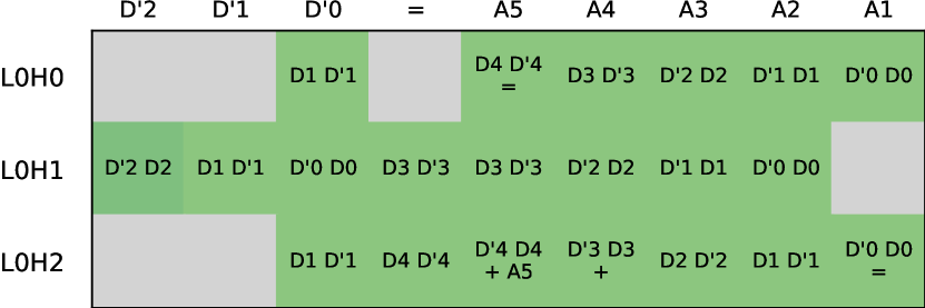
Figure 5: This map shows the input tokens each attention head attends to at each token position. At token position P11 (token =) the model predicts the first answer digit A5. All digit pairs (e.g. D2 D’2) are attended to by P11.

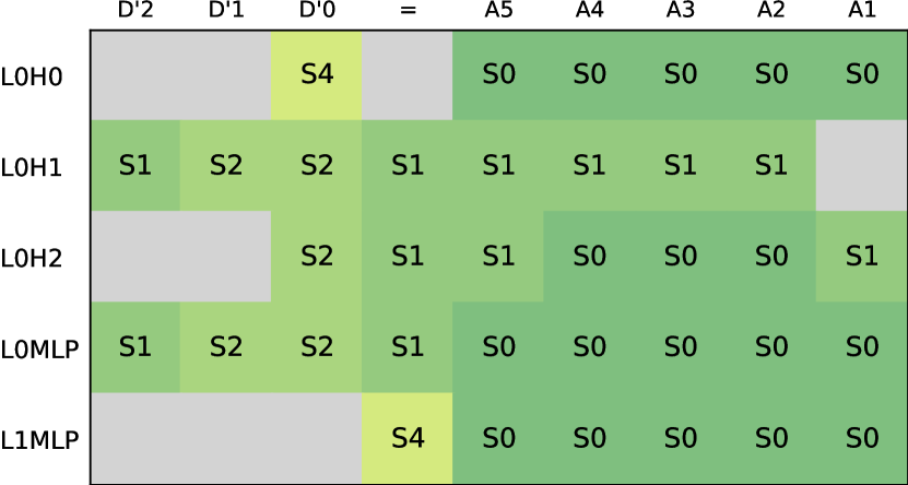
Figure 6: This map shows the lowest complexity quanta S0, S1, etc impacted when we ablate each node in the 5-digit 2-layer 3-head addition model. To answer S0 questions, only the S0 nodes are used. To answer S1 questions, S0 and S1 nodes are used, etc.

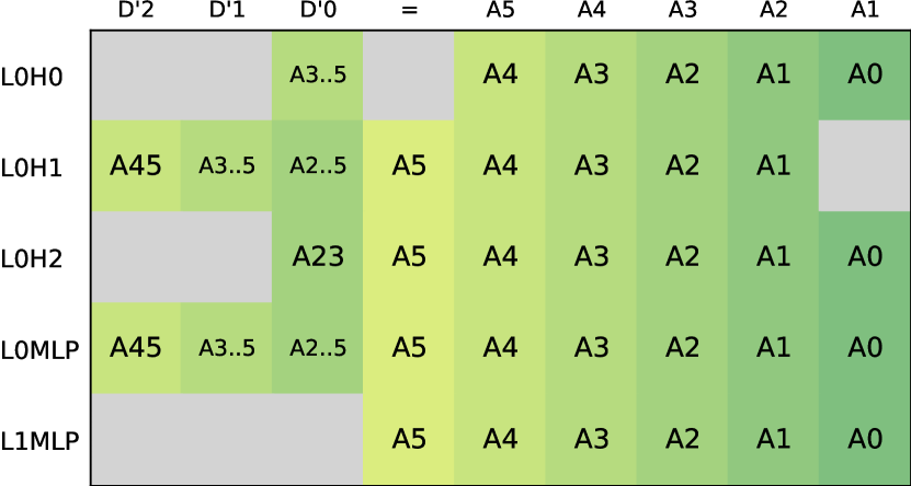
Figure 7: This map shows the answer digit(s) A0 .. A5 impacted when we ablate each useful node in the 5-digit 2-layer 3-head addition model. The “column per digit” pattern in the last 6 columns mirrors the 1-layer model’s pattern. Cells containing values like A2..5 (in column D’0) are used in multiple prediction steps to calculate multiple answer digits e.g. A2 to A5.

The algorithm predicts the first answer digit, A5, at position P11 (tokne =). This digit, which can only be 0 or 1, is the most challenging to predict as it may rely on a cascade starting from the digit pair D0 D’0 (e.g., 55555+44445=100000). The algorithm is required to compute this cascade using the nodes located in positions P8 to P11 (input tokens D’2 to =). As illustrated in Figure 5, these nodes attend to all digit pairs from D4 D’4 to D0 D’0 by P11. Additionally, the PCA data, as shown in Figures 13 and 14, suggest that these nodes produce tri-state outputs.

After encountering several initial setbacks (see App. E and F), we discovered that the model utilizes a minimal set of “make carry” information, leading to the development of the TriCase quanta.

The model performs $D_{n}.C$ using bigrams (see App. D) to map two input tokens to one result token e.g. “6” + “7” = T10. In positions P8 to P11, the model does $D_{n}.C$ calculations on all digit pairs from D4 D’4 to D0 D’0.

The mathematical framework behind this is intricate. To validate it, we implemented the algorithm in Python and successfully executed one million additions with zero errors.

For a specific instance of the 5-digit addition model, we mapped the algorithm to individual nodes. Using ablation interventions, we verified each node’s role in executing the expected algorithmic step (see App. G). Table 2 and Figure 1 illustrate how the algorithm was applied to this particular model instance, adhering to all known constraints and accurately calculating all six answer digits.

Table 2: Pseudo-code for accurately predicting all answer digits, with mappings to the model nodes that implement the pseudo-code, for a specific 5-digit model instance.

Value	Value calculated as	Nodes used
D2.C	TriCase(D2, D’2)	P8.L0.H1 and P8.L0.MLP
D1.C	TriCase(D1, D’1)	P9.L0.H1 and P9.L0.MLP
D1.C2	TriAdd(D1.C, TriCase(D0, D’0))	P10.L0.H1 and P10.L0.MLP
D3.C4	TriAdd(TriCase(D3, D’3), TriAdd(D2.C,D1.C2))	P11.L0.H1
D4.C	TriCase(D4, D’4)	P11.L0.H2
D4.C5	TriAdd(D4.C, D3.C4)	P11.L0.MLP
A5	(D4.C5 == 10)	P11.L1.MLP
D4.BA	(D4 + D’4) % 10	P12.L0.H0 + H2
D3.C4	TriAdd(TriCase(D3, D’3), TriAdd(D2.C,D1.C2))	P12.L0.H1
A4	(D4.BA + (D3.C4 / 10)) % 10	P12.L0.MLP and P12.L1.MLP
D3.BA	(D3 + D’3) % 10	P13.L0.H0 + H2
D2.C3	TriAdd(D2.C,D1.C2)	P13.L0.H1
A3	(D3.BA + (D2.C3 / 10)) % 10	P13.L0.MLP and P13.L1.MLP
D2.BA	(D2 + D’2) % 10	P14.L0.H0 + H2
D1.C2	(D1 + D’1) / 10 + P10.D1.C2 *	P14.L0.H1
A2	(D2.BA + (D1.C2 / 10)) % 10	P14.L0.MLP and P14.L1.MLP
D1.BA	(D1 + D’1) % 10	P15.L0.H0 + H2
D0.MC	(D0 + D’0) / 10	P15.L0.H1
A1	(D1.BA + D0.MC) % 10	P15.L0.MLP and P15.L1.MLP
A0	(D0 + D’0) % 10	P16.L0.H0 + H2 P16.L0.MLP and P16.L1.MLP

Throughout the training of different instances of the 5-digit models, small modifications to the training environment resulted in subtly varied implementations. All variations seen use the Figure 3 algorithm, but each has small implementation differences. For example, in positions P8 to P11, the model might alter which 5 nodes perform the $D_{n}.C$ calculations and in what order. This corresponds to small changes in the Tab. 2 documentation per variation.

In summary, we concluded that the specific instance of the 5-digit addition model documented above is reliably accurate, well-understood, well-functioning and so known-good.

4.2 Case Study: Extending to Six-Digit Addition

Our investigations showed that all instances of the 5-digit addition model we trained appeared to utilize the same algorithm. To determine if this algorithm extends to related models, we trained a 6-digit 2-layer 3-head addition model, employing a different seed and optimizer. Additionally, we modified the answer format to include a ’+’ token (e.g., 111111+222222=+0333333).

Employing similar quanta and training data enrichment techniques, we developed a 6-digit addition model. This model achieved a loss of approximately $9.1\times 10^{-9}$ and demonstrated 1M Q accuracy.

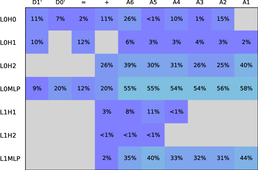
Figure 15: This map shows the % of questions that fail when we ablate each node in the 6-digit 2-layer 3-head addition model. The model only uses nodes in token positions P11 to P20. Lower percentages correspond to rarer edge cases. The grey space represents nodes that are not useful.

The 5-digit (see Figures 4,  5,  6, and  7) and 6-digit (see Figures 15,  16,  8, and  17) quanta maps show numerous similarities, suggesting the 6-digit model implements the logical extension of the 5-digit algorithm (see Figure 3).

Intervention ablation tests show the 6-digit model does 6 BA and 6 MC calculations in late tokens, and does 6 $D_{n}.C$ calculations in early tokens with PCA showing the expected TriCase output. The 5 $D_{n}$.$C_{m}$ calculations are still to be tested.

Give this model has 1M Q accuracy, if this testing is successfully completed, and the algorithm implementation detail is documented, we can state the 6-digit model is known-good.

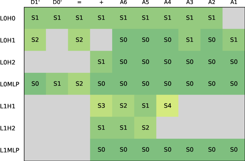
Figure 8: This map shows the simpliest addition complexity quanta S0, S1, etc used in each useful node of the 6-digit 2-layer 3-head addition model. Note the similarity to 5-digit Figure 6

4.3 Case Study: Extending the model for subtraction

To explore the reuse of known-good models, we developed a larger (6-digit 3-layer 4-head) model capable of performing both addition and subtraction. We introduced specific subtraction quanta and enriched the training dataset with rare subtraction edge cases.

This new “mixed” model, initially untrained, was initialized with the weights from the (6-digit 2-layer 3-head) addition model. To facilitate its learning of subtraction while maintaining its pre-inserted addition skills, we trained the mixed model with a dataset comprising 80% subtraction and 20% addition problems. This approach resulted in a model achieving 1M Q accuracy for both addition and subtraction tasks. Attempts to “freeze” useful attention heads and/or MLP layers from the addition model by periodically copying their weights back into the mixed model every 100 training epochs, however, led to decreased accuracy.

Subtraction ($a-b$) presents a greater challenge than addition ($a+b$), primarily due to its two distinct cases: $a>b$ (positive answer) and $a<b$ (negative answer). The model must discern this difference to accurately determine the first answer token as either “+” or “-”.

In cases of “positive” subtraction, the process closely mirrors addition. This observation led us to define subtraction quanta (see Tables 3 and 4 (see App. J), paralleling the addition quanta.

Calculating the “-” case in subtraction is more complex than the “+” case. The model might employ distinct circuits for each scenario. Our hypothesis is that after mastering the simpler “+” case, the model will learn to apply the mathematical identity $a-b=-(b-a)$, thus enabling it to handle “-” case questions by re-utilizing the “+” case circuits and then inverting the result. To examine this, we introduced the NG quanta (see Table 4) and again applied mean-ablation techniques to analyze the process.

Table 3: We categorise digit-pair differences (i.e. $D_{n}$- $D^{\prime}_{n}$ abbreviated as $D_{n}$.Diff) into three groups. These subtraction groups parallel the BA, MC and US addition groups. Groups BS and DZ overlap.

Name	Abbrev	Definition	E.g.	Like
Base Subtract	BS	$D_{n}$.Diff $<=0$	7 - 2	BA
Borrow 1	B1	$D_{n}$.Diff $<0$	7 - 9	MC
Diff Zero	DZ	$D_{n}$.Diff = 0	7 - 7	US

Table 4: We categorise subtraction questions into non-overlapping “calculation complexity” quanta, ordered by increased computational difficulty and decreasing occurrence frequency. Five-digit subtraction questions quanta are M0 to M4. Ten-digit subtraction question quanta are M0 to M9, and M9’s frequency is $\sim$0.000001%. Subtraction questions where the answer is negative get their own category NG .

Name	Contains	Example	Freq
M0	BS	33333-22222=+11111	$\sim$25%
M1	BS,B1	33333-22282=+11051	$\sim$15%
M2	BS,B1,DZ	33333-22382=+10951	$\sim$8%
M3	BS,B1,DZx2	33333-23382=+09951	$\sim$2%
M4	BS,B1,DZx3	33333-23338=+09995	$\sim$0.1%
NG	N/A	10000-90000=-80000	$\sim$50%

We compared the nodes utilized by the inserted addition model (see Figure 6) to those used by the mixed model when performing addition (see Figure 9). There is a strong correlation between them. Notably, the mixed model predominantly uses the existing attention heads in layers 1 and 2, ignoring many available spare heads.

Further comparison was made between the nodes the mixed model employs for addition and subtraction (see Figures 9 and 10). The nodes used for addition (S*) and those for “subtraction with a positive answer” (M*) show a very strong correlation. This suggests that the model repurposes its addition nodes to facilitate subtraction in some manner. Notably, an additional 15 nodes are activated for subtraction problems that result in a negative answer (represented by the NG quanta).

While the mixed model has 1M Q accuracy for both addition and subtraction tasks, intervation ablation testing and PCA of the mixed model have not been completed, and the algorithm implementation has not been documented. We cannot yet assert that it is known-good.

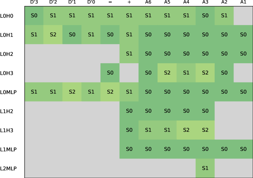
Figure 9: This map shows the simplest complexity quanta S0, S1, etc used in each useful node of the 6-digit 3-layer 4-head mixed model when doing addition questions.

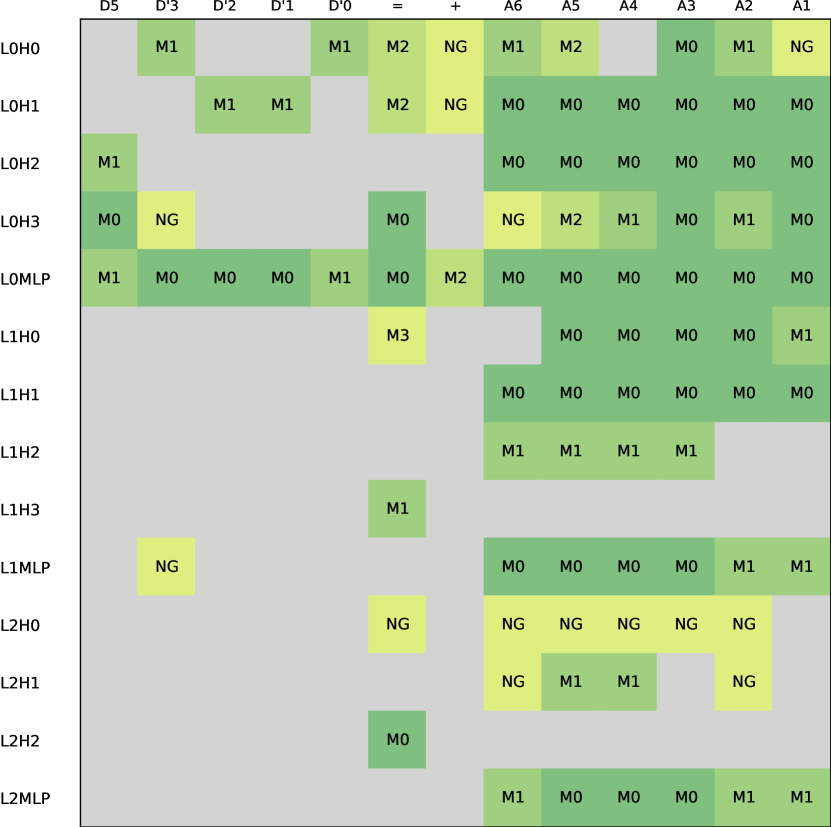
Figure 10: This map shows the simpliest complexity quanta M0, M1, etc used in each useful node of the 6-digit 3-layer 4-head mixed model for subtraction questions with positive answers. The NG cells are only used in subtractions $a-b$ where $a<b$, likely implementing the $-(b-a)$ identity as described in  4.3.

5 Conclusion

In this paper, we successfully trained a 5-digit 2-layer 3-head addition model that we have verified as known-good. Our investigation revealed that a 6-digit 2-layer 3-head addition model follows the same algorithmic principles, albeit with some implementation variations.

A significant aspect of our work was demonstrating component reuse. We achieved this by integrating an existing addition model into a new “mixed” model designed for both addition and subtraction tasks. This integration allowed us to leverage our in-depth understanding of the addition model’s algorithm to unravel the workings of the mixed model. Our findings indicate that the mixed model employs the nodes of the inserted addition model for conducting both addition and subtraction computations.

This paper lends support to the assertion by Michaud et al. (2023) that many natural prediction problems can be broken down into a finite set of “quanta” computations. These quanta are essential for models to learn in order to minimize loss. Furthermore, it aligns with the concept that comprehending a network’s functionality is fundamentally about identifying and understanding its sub-quanta.

6 Limitations and Future Work

Our research opens up several promising avenues for future exploration. A key objective is to establish the mixed model as known-good by reverse-engineering its algorithm implementation and validating it through experimental methods. Additionally, we aim to develop a comprehensive model that proficiently handles addition, subtraction, multiplication, and division, ensuring its status as known-good.

Currently, our approach requires significant human effort, which may not be feasible for large-scale applications. However, we believe applying this method to critical tasks, such as logical reasoning involving both simple (e.g., AND, OR) and more complex operators (e.g., Converse, Inverse), is justified. This could lead to the creation of more known-good transformer models, potentially extending to frameworks for ethical decision-making.

A promising finding of our research was the successful insertion of a known-good model into a larger, untrained model while retaining its functionality. We think it might be feasible to embed a compact known-good model into an existing Large Language Model (LLM) to enhance its trustworthiness. Previous studies (Stolfo et al., 2023; Kruthoff, 2024) found nodes in LLMs that were responsible for inaccuracies mathematical calculations. Given our findings, it might be possible to replace these nodes with known-good ones. While this poses an engineering challenge, research by (Voita et al., 2023) and (Hu et al., 2021) indicates the presence of “spare” neurons in LLMs and the potential for integrating small-scale modifications to fix erroneous circuits in LLMs.

Moreover, developing methods to incorporate compact known-good models into LLMs, whether untrained or trained, could democratize AI Safety research. It enables small teams to focus on specific functional areas, crafting component models to a defined quality standard for integration into various LLMs.

A significant challenge in our research was the sensitivity of model behavior to minor changes in the training environment. These changes often altered the specific nodes used for calculations, necessitating manual adjustments to our algorithm-validation test suite. A more effective strategy would be a declarative approach to describing each component in an algorithm hypothesis, allowing automatic identification of corresponding model nodes. For instance, a component description could specify nodes that primarily attend to question digits D2 and D’2, influence answer digit A3, and are crucial for S0 but not S1 complexity questions. Such a declarative language and its accompanying tooling would accelerate research progress and ensure that known-good components retain their functionality when integrated into LLMs. An initial version of this tooling has been created, but significant further work is required to fully realize its potential.

Impact Statement

Our work aims to explain the inner workings of transformer-based language models, which may have broad implications for a wide range of applications. A deeper understanding of generative AI has dual usage. While the potential for misuse exists, we discourage it. The knowledge gained can be harnessed to safeguard systems, ensuring they operate as intended. It is our sincere hope that this research will be directed towards the greater good, enriching our society and preventing detrimental effects. We encourage responsible use of AI, aligning with ethical guidelines.

Appendix A Appendix: Model Configuration

Addition experiments were done in Colab notebooks named “Accurate Addition - Train” and “Accurate Addition - Analyse”. They run on a T4 GPU. Training takes $\sim$15 mins. Analysis takes $\sim$8 mins. The key parameters (which are all configurable) are:

• n_layers = 2: This is a 2-layer Transformer model

• n_heads = 3: There are 3 attention heads

• n_digits = 5: Number of digits in the addition question

Training uses a new batch of data each step (aka Infinite Training Data) to minimise memorisation. During a training run the model processes about 1.5 million training datums. For the 5-digit addition problem there are 100,000 squared (that is 10 billion) possible questions. So the training data is much less than 1% of the possible problems. Because US cascades (e.g. 44445+55555=100000, 54321+45679=1000000, 44450+55550=10000, 1234+8769=10003) are exceedingly rare, the data generator was enhanced to increase the likelihood of these cases turning up in the training data

Mixed operation (addition and subtraction) experiments were done in Colab notebooks named “Accurate Math - Train” and “Accurate Math - Analyse”. They run on a T4 GPU. Training takes $\sim$25 mins. Analysis takes $\sim$8 mins. The key parameters (which are all configurable) are:

• n_layers = 3: This is a 3-layer transformer model

• n_heads = 4: There are 4 attention heads

• n_digits = 6: Number of digits in the addition and subtraction questions

Training uses a new batch of data each step (aka Infinite Training Data) to minimise memorisation.

In all Colabs, each digit is represented as a separate token. (Liu & Low, 2023) state that LLaMa’s “remarkable arithmetic ability … is mainly atributed to LLaMA’s consistent tokenization of numbers”.

These Colabs are available at https://github.com/apartresearch/Verified_Addition

Appendix B Appendix: Addition Model Loss

The 1-layer model is not very accurate (see Tab. 5). With 2 layers the model gains accuracy (see Tab. 6). The model uses batch_size = 64, n_heads = 3, lr = 0.00008, weight_decay = 0.1. The loss function is simple:

• Per Digit Loss: For “per digit” graphs and analysis, for a given answer digit, the loss used is negative log likelihood.

• All Digits Loss: For “all answer digits” graphs and analysis, the loss used is the mean of the “per digit” loss across all the answer digits.

Table 5: Results for 1-layer 3-head model with 5, 10 & 15 digits

No. digits	5	10	15
Training batches	20K	20K	20K
Loss	0.008314	0.040984	0.031746
Heads used	15	29	46
MLPs used	6	11	16

Table 6: Results for 2-layer 3-head model with 5 & 10 digits

No. digits	5	5	10	10
Training batches	20K	30K	20K	30K
Loss	2.7e-6	2.3e-8	9.4e-5	1.2e-4
Heads used	21	19	57	51
MLPs used	15	15	27	28

The 2-layer, 5-digit model trained over 30 thousand batches has a final training loss of $\sim 2.3\times 10^{-8}$.

Appendix C Appendix: Addition Model Shape Choice

While we wanted a very low loss addition model, we also wanted to keep the model compact - intuiting that a smaller model would be easier to understand than a large model. Here are the things we tried to reduce loss that didn’t work:

• Increasing the frequency of hard (cascading US ) examples in the training data so the model has more hard examples to learn from. This improved training speed but did not reduce loss.

• Increasing the number of attention heads from 3 to 4 or 5 (while still using 1 layer) to provide more computing power.

• Changing the question format from “12345+22222=” to “12345+22222equals” giving the model more prediction steps after the question is revealed before it needs to state the first answer digit.

• With n_layers = 1 increasing the number of attention heads from 3 to 4.

• Changing the n_layers to 2 and n_heads to 2.

The smallest model shape that did reduce loss significantly was 2 layers with 3 attention heads

Appendix D Appendix: TriAdd Implementation

TriAdd transfers data from $(D_{n-1})$ to $(D_{n})$ by integrating the values of $(D_{n}.C)$ and $(D_{n-1}.C)$. This function can be represented as nine bigram mappings with three possible outputs.

Table 7: $D_{n}$.TriAdd can be calculated from $D_{n}.C$ and $D_{n-1}.C$ through nine bigram mappings and yielding the three distinct outputs T8, T9 and T10

	$D_{n}.C$ =T8	$D_{n}.C$ =T9	$D_{n}.C$ =T10
$D_{n-1}.C$ = T8	T8	T9	T10
$D_{n-1}.C$ = T9	T8	T9	T10
$D_{n-1}.C$ = T10	T9 *	T10	T10

Note that in the case $D_{n}.C$ = T9 and $D_{n-1}.C$ = T10, the answer is indeterminate. The result could be T8 or T9 but importantly it can not be T10. We choose to use T9 in our definition, but T8 would work just as well.

Appendix E Appendix: Addition Hypothesis 1

Given the 2-layer attention pattern’s similarity to 1-layer attention pattern, and the above evidence, our first (incorrect) hypothesis was that the 2-layer algorithm:

• Is based on the same BA, MC and US operations as the 1-layer.

• Uses the new early positions to (somehow) do the US calculations with higher accuracy than the 1-layer model.

• The long double staircase still finalises each answer digit’s calculation.

• The two attention nodes in the long double staircase positions do the BA and MC calculations and pull in US information calculated in the early positions.

If this is correct then the 2-layer algorithm successfully completes these calculations:

• A0 = D0.BA

• A1 = D1.BA + D0.MC

• A2 = D2.BA + (D1.MC or (D1.MS & D0.MC))

• A3 = D3.BA + (D2.MC or (D2.MS & D1.MC) or (D2.MS & D1.MS & D0.MC))

• A4 = D4.BA + (D3.MC or (D3.MS & D2.MC) or (D3.MS & D2.MS & D1.MC) or (D3.MS & D2.MS & D1.MS & D0.MC))

• A5 = D4.MC or (D4.MS & D3.MC) or (D4.MS & D3.MS & D2.MC) or (D4.MS & D3.MS & D2.MS & D1.MC) or (D4.MS & D3.MS & D2.MS & D1.MS & D0.MC)

Our intuition is that there are not enough useful nodes in positions 8 to 11 to complete the A5 calculation this way. So we abandoned this hypothesis.

Appendix F Appendix: Addition Hypothesis 2

Our second (incorrect) hypothesis was that the 2-layer algorithm has a more compact data representation, so it can pack more calculations into each node, allowing it to accurately predict A5 in step 11.

We claimed the model stores the sum of each digit-pair as a single token in the range “0” to “18” (covering 0+0 to 9+9). We name this operator $D_{n}$.T, where T stands for “token addition”:

• $D_{n}$.T = $D_{n}$+ $D^{\prime}_{n}$

The $D_{n}$.T operation does not understand mathematical addition. Tab. 8 shows how the model implements the T operator as a bigram mapping.

Table 8: Implementing the T operator as a bigram mapping from 2 input tokens to 1 result token.

$D_{n}$vs $D^{\prime}_{n}$	0	1	…	4	5	…	8	9
0	0	1	…	4	5	…	8	9
1	1	2	…	5	6	…	9	10
…	…	…	…	…	…	…	…	…
4	4	5	…	8	9	…	12	13
5	5	6	…	9	10	…	13	14
…	…	…	…	…	…	…	…	…
8	8	9	…	12	13	…	16	17
9	9	10	…	13	14	…	17	18

$D_{n}$.T is a compact way to store data. Tab. 9 show how, if it needs to, the model can convert a $D_{n}$.T value into a one-digit-accuracy BA, MC or MS value.)

Table 9: Converting a $D_{n}$.T value into a BA , MC or MS value.

$D_{n}$.T	$D_{n}$.BA	$D_{n}$.MC	$D_{n}$.MS
0	0	0	0
1	1	0	0
…	…	…	…
8	8	0	0
9	9	0	1
10	0	1	0
…	…	…	…
17	7	1	0
18	8	1	0

Our notation shorthand for one-digit-accuracy these “conversion” bigram mappings is:

• $D_{n}$.BA = ($D_{n}$.T % 10) where % is the modulus operator

• $D_{n}$.MC = ($D_{n}$.T // 10) where // is the integer division operator

• $D_{n}$.MS = ($D_{n}$.T == 9) where == is the equality operator

The D0.T value is perfectly accurate. But the other $D_{n}$.T values are not perfectly accurate because each is constrained to information from just one digit. We define another more accurate operator $D_{n}$.T2 that has “two-digit accuracy”. $D_{n}$.T2 is the pair sum for the nth digit plus the carry bit (if any) from the n-1th digit T:

• $D_{n}$.T2 = $D_{n}$.T + $D_{n-1}$.MC

$D_{n}$.T2 is more accurate than $D_{n}$.T. The $D_{n}$.T2 value is always in the range “0” to “19” (covering 0+0+0 to 9+9+MakeCarry). Tab. 10 show how the model can implement the T2 operator as a mapping.

Table 10: Calculating $D_{n}$.T2 from $D_{n}$.T and $D_{n-1}$.T

$D_{n}$.T	$D_{n}$.T2 if $D_{n-1}$.MC==0	$D_{n}$.T2 if $D_{n-1}$.MC==1
0	0	1
1	1	2
…	…	…
9	9	10
10	10	11
…	…	…
17	17	18
18	18	19

Following this pattern, we define operators $D_{n}$.T3, $D_{n}$.T4 and $D_{n}$.T5 with 3, 4 and 5 digit accuracy respectively:

• $D_{n}$.T3 = $D_{n}$.T + ( $D_{n-1}$.T2 // 10 ) aka $D_{n}$.T + $D_{n-1}$.MC2

• $D_{n}$.T4 = $D_{n}$.T + ( $D_{n-1}$.T3 // 10 ) aka $D_{n}$.T + $D_{n-1}$.MC3

• $D_{n}$.T5 = $D_{n}$.T + ( $D_{n-1}$.T4 // 10 ) aka $D_{n}$.T + $D_{n-1}$.MC4

The value D4.T5 is perfectly accurate as it integrates MC and cascading MS data all the way back to and including D0.T. The values D1.T2, D2.T3, D3.T4 are also all perfectly accurate. If the model knows these values it can calculate answer digits with perfect accuracy:

• A1 = D1.T2 % 10 with zero loss

• A2 = D2.T3 % 10 with zero loss

• A3 = D3.T4 % 10 with zero loss

• A4 = D4.T5 % 10 with zero loss

• A5 = D4.T5 // 10 with zero loss

Tab. 11 shows how the hypothesis 2 mathematical framework is applied and Figure 11 shows how this maps to the model. There are nodes that the model needs that this framework does not use, so our hypothesis is not 100% right.

Table 11: Accurately predicting A5 in step 11 and A4 in step 12 using addition hypothesis 2

Calculation	Node
D1.T = D1 + D’1	P9.L0.H1 and P9.L0.MLP
D2.T = D2 + D’2	P8.L0.H1 and P8.L0.MLP
D1.T2 = D2.T + (D1.T + (D0 + D0’) // 10) // 10	P10.L0.H1 and P10.L0.MLP
D3.T4 = D3 + D’3 + D2.T3 // 10	P11.L0.H1
D4.T = D4 + D’4	P11.L0.H2
D3.MC3 = D3.T4 // 10	P11.L0.MLP
A5 = (D4.T + D3.MC3) // 10	P11.L1.MLP
D4.T5 = D4.T + D3.T4 // 10	P12.L0.H0
A4 = D4.T5 % 10 // 10	P12.L0.MLP

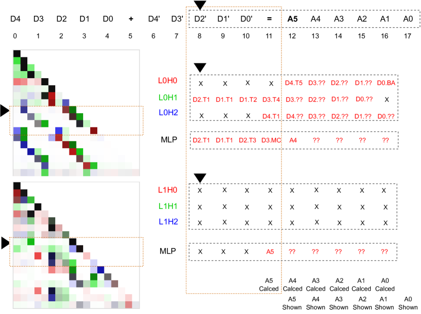
Figure 11: The 5-digit 2-layer integer addition model algorithm under hypothesis 2

In this hypothesis, all the answer digits are perfectly calculated using the nodes in positions 8 to 11. This hypothesis 2 is feasible, elegant and compact - reflecting the authors (human) values for good code.

Experimenation shows the model does not implement this hypothesis. It retains the long staircase BA calculations in positions 11 to 16. Why? Two reasons suggest themselves:

• Hypothesis 2 is too compact. The model is not optimising for compactness. The long staircase is discovered early in training, and it works for simple questions. Once the overall algorithm gives low loss consistently it stops optimising.

• Hypothesis 2 accurately predicts all answer digits in step 11 - reflecting the authors (human) values for good code. The model is not motivated to do this. It just needs to accurately predict A5 as 1 or 0 in step 11 and A4 in step 12 - nothing more.

We abandoned this hypothesis.

Appendix G Appendix: Five-Digit Addition Experiments

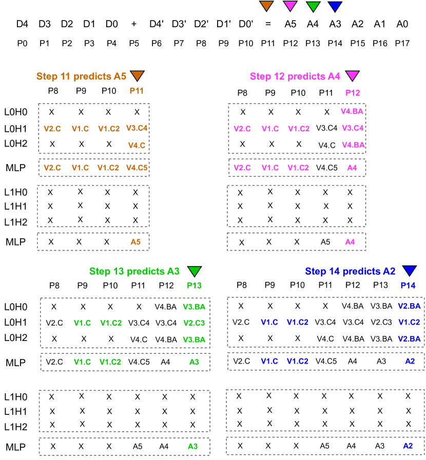
Figure 12: Our 5-digit integer addition question has 12 question tokens ($D_{n}$,$D^{\prime}_{n}$) followed by 6 answer tokens ($A_{n}$). This known-good 2-layer 3-head model can perform one million predictions without error. The model’s algorithm co-ordinates computation across 9 token positions ($P_{n}$) using 19 attention heads ($H_{n}$) and 15 MLP layers. Three attention heads produce intermediate results that are reused in multiple prediction steps e.g. P10.L0.H1 is reused in 4 prediction steps to calculate answer digits A5 to A2.

The hypothesis 3 pseudo-code was derived iteratively by obtaining experimental results and mapping them to mathematical operations. Figure 12 shows the pseudo-code diagramtically. Some of the experiments and mappings were:

• Ablation experiments show that the A5 value is accurately calculated in prediction step 11 using 5 attention heads and 5 MLP layers. The pseudo-code accurately calculates A5 while constraining itself to this many steps.

• Ablating the nodes one by one shows which answer digit(s) are reliant on each node (Ref Figure 7). Most interestingly, ablating P10.L0.H1 impacts the answer digits A5, A4, A3, A2 (but not A1 and A0). This node is used in the calculation of A5, A4, A3, A2 in prediction steps 11, 12, 13 and 14. These relationships are constraints that are all obeyed by the pseudo-code.

• The pseudo-code has 4 instances where $D_{n}.C$ is calculated using TriCase. PCA of the corresponding nodes (P8.L0.H1, P9.L0.H1, P11.L0.H2 and P14.L0.H1) shows tri-state output for the specified $D_{n}$. (see Figure 13).

• The pseudo-code has 4 instances where compound functions using TriCase and TriAdd to generate tri-state outputs. PCA of the corresponding nodes (P11.L0.H1, P12.L0.H1 and P13.L0.H1) shows tri-state output for the specified $D_{n}$. (see Figure 13).

• Activation patching (aka interchange intervention) experiments at attention head level confirmed some aspects of the calculations (see § H for details.

• The pseudo code includes calculations like D1.C which it says is calculated in P9.L0.H1 and P9.L0.MLP. Ablation tells us both nodes are necessary. For the attention head we use the PCA results for insights. We didn’t implement a similar investigative tool for the MLP layer, so in the pseudo-code we attribute the calculation of D1.C to both nodes.

• For P10.L0.H1, the attention head PCA could represent either a bi-state or tri-state output (see Figure 14). The MLP layer at P10.L0.MLP could map the attention head output to either a bi-state or tri-state. We cannot see which. The pseudo-code shows a tri-state calculation at P10.L0.MLP, but with small alterations the pseudo-code would work with a bi-state output.

• For P15.L0.H1 the attention head PCA could represent either a bi-state or tri-state output (see Figure 14). The pseudo-code shows a bi-state calculation D0.MC at P15.L0.H1, but with small alterations the pseudo-code would work with a tri-state output.

• The calculation of D1.C2 in P14.L0.H1 is a interesting case. The model needs D1.C2 for A2 accuracy. The model could simply reuse the accurate D1.C2 value calculated in P10. Activation patching shows that it does not. Instead the P14 attention heads calculate D1.C1 from D1 and D’1 directly, and only relies on the P10.D1.C2 value in the case where D1.C2 != D1.C. That is, the calculation is “use P14.D1.C1 value else use P10.D1.C2 values”. This aligns with the model learning the P10.D1.C calculation early in training (for 90% accuracy) and later learning that P10.D1.C2 contains additional information it can use to get to 100% accuracy.

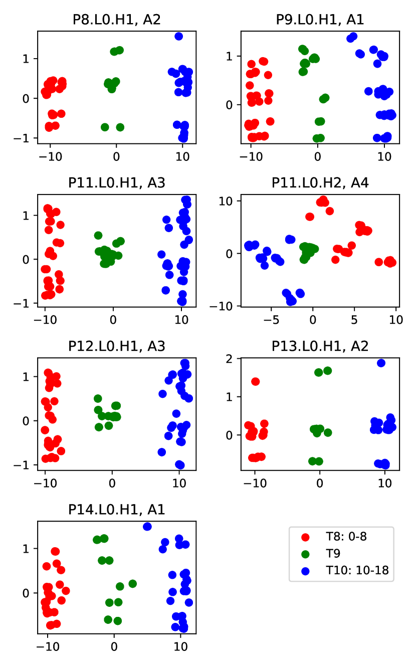
Figure 13: For 5-digit addition, for these attention heads, for exactly 1 answer digit $A_{n}$each, PCA shows these interpretable results. The dot colours show the TriCase value of each question. The PCA data and TriCase quanta are both tri-state and strongly correlated.

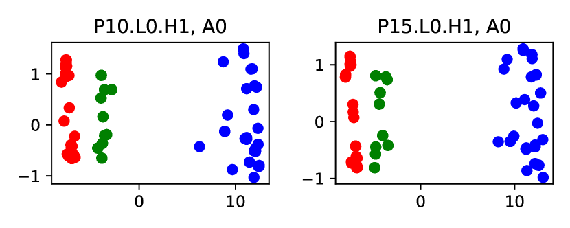
Figure 14: For 5-digit addition, for these attention heads, for exactly 1 digit $A_{n}$each, PCA shows these interpretable results. The dot colours show the TriCase value of each question. The PCA and TriCase data are strongly correlated, but the PCA data has 2 states.

Appendix H Appendix: Addition Interchange Interventions

To test the hypothesis 3 mapping of the mathematical framework (casual abstraction) to the model attention heads, various “interchange interventions” (aka activation patching) experiments were performed on the model, where

• A particular claim about an attention head has selected for testing.

• The model predicted answers for sample test questions, and the attention head activations were recorded (stored).

• The model then predicted answers for more questions, but this time we intervened during the prediction to override the selected attention head activations with the activations from the previous run.

Using this approach we obtained the findiings in Tab. 12.

Table 12: Interchange Interventions experiments used activation patching to test the claims addition hypothesis 3 made for each attention head. Experimental results are consistent with hypothesis 3 for all nodes.

Nodes	Claim: Attention head(s) perform …	Finding: Attention head(s) perform a function that …
P8.L0.H1 and MLP	D2.C = TriCase( D2, D’2 ) impacting A4 and A5 accuracy	Based on D2 and D’2. Triggers on a D2 carry value. Provides carry bit used in A5 and A4 calculation.
P9.L0.H1 and MLP	D1.C = TriCase( D1, D’1 ) impacting A5, A4 and A3 accuracy	Based on D1 and D’1. Triggers on a D1 carry value. Provides carry bit used in A5, A4 and A3 calculation.
P10.L0.H1 and MLP	D1.C2 = TriAdd( D1.C, TriCase(D0, D’0) ) impacting A5, A4, A3 and A2 accuracy	Based on D0 and D’0. Triggers on a D0 carry value. Provides carry bit used in A5, A4, A3 and A2 calculation.
P11.L0.H1 and MLP	D3.C4 = TriAdd( TriCase( D3, D’3 ), TriAdd( D2.C, D1.C2)) impacting A5 accuracy	Based on D3 and D’3. Triggers on a D3 carry value. Provides carry bit used in A5 calculations.
P11.L0.H2 and MLP	D4.C = TriCase(D4, D’4) impacting A5 accuracy A4	Based on D4 and D’4. Triggers on a D4 carry value. Provides carry bit used in A5 calculation.
P12.L0.H0+H2 and MLP	D4.BA = (D4 + D’4) % 10 impacting A4 accuracy A4	Sums D4 and D’4. Impacts A4.
P13.L0.H0+H2 and MLP	D3.BA = (D3 + D’3) % 10 impacting A3 accuracy	Sums D3 and D’3. Impacts A3.
P14.L0.H0+H2 and MLP	D2.BA = (D2 + D’2) % 10 impacting A2 accuracy	Sums D2 and D’2. Impacts A2.
P14.L0.H1 and MLP	(D1 + D’1) / 10 + P10.D1.C2 info impacting A2 accuracy	Calculates P10.D1.C1 but add P10.D1.C2 info when D1.C != D1.C2. Impacts A2
P15.L0.H0+H2 and MLP	D1.BA = (D1 + D’1) % 10 impacting A1 accuracy	Sums D1 and D’1. Impacts A1.
P15.L0.H1 and MLP	D0.MC = (D0 + D’0) / 10 impacting A1 accuracy	Triggers when D0 + D’0 >10. Impacts A1 digit by 1
P16.L0.H0+H2 and MLP	D0.BA = (D0 + D’0) % 10 impacting A0 accuracy	Sums D0 and D’0. Impacts A0.

Appendix I Appendix: Six-Digit Addition

We trained a very low loss 6-digit Addition model. We compared the 5-digit and 6-digit model algorithms. Figures 6 and  8 are very instructive. So are Figures 7 and  17. We concluded that the 6-digit model used the same logical algorithm as the 5-digit model. There were some implementation differences:

• The models selected different attention heads in the early positions to use to do the same logical calculations.

• The 5-digit model used 2 attention heads per digit to do the BA calculation, whereas 6-digit model only uses one (and so is more compact).

• The PCA trigrams have difference appearances in the two models. Figures 13 and  18.

• For 6-digits, for A2 (only), the BA calculation is done in P18, but the MC calculation is not in P18. This is unique. The 6-digit model has optimised out the MC and instead relies solely on the accurate D1.C2 value (and so is more compact).

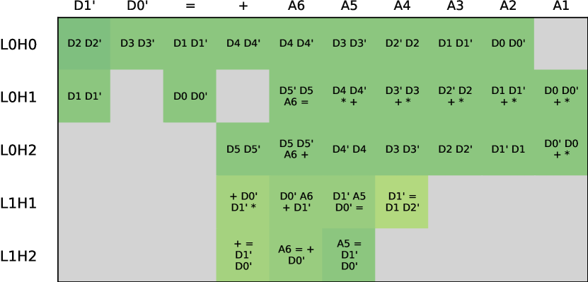
Figure 16: This map shows the input tokens each attention head attends to at each token position. The model predicts the first answer digit A6 in token position P14, and all digit-pair sums (e.g. D2 D’2) are attended to in P11 to P14. Note the similarity to Figure 5.

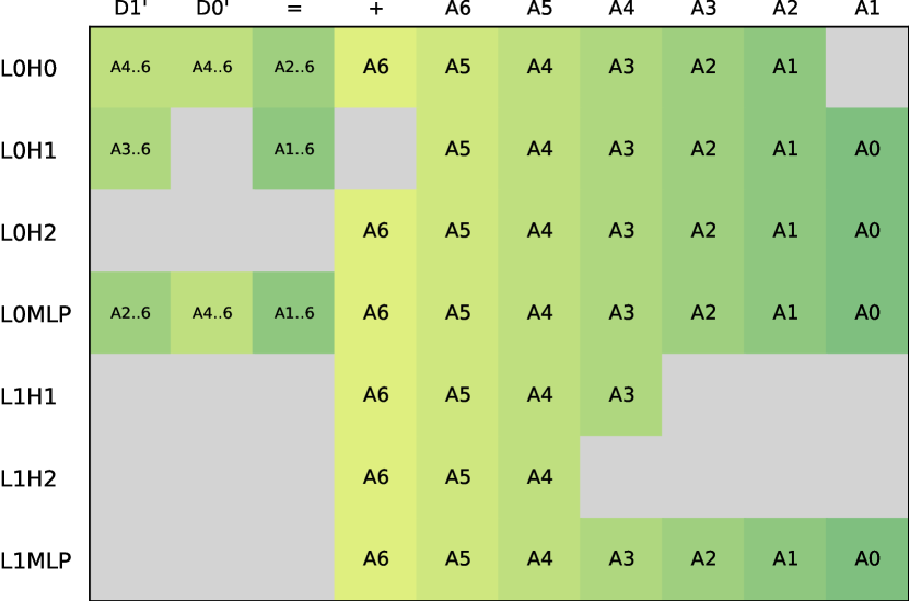
Figure 17: This map shows the answer digit(s) A0 .. A5 impacted when we ablate each useful node in the 6-digit 2-layer 3-head addition model. Note the similarity to Figure 7.

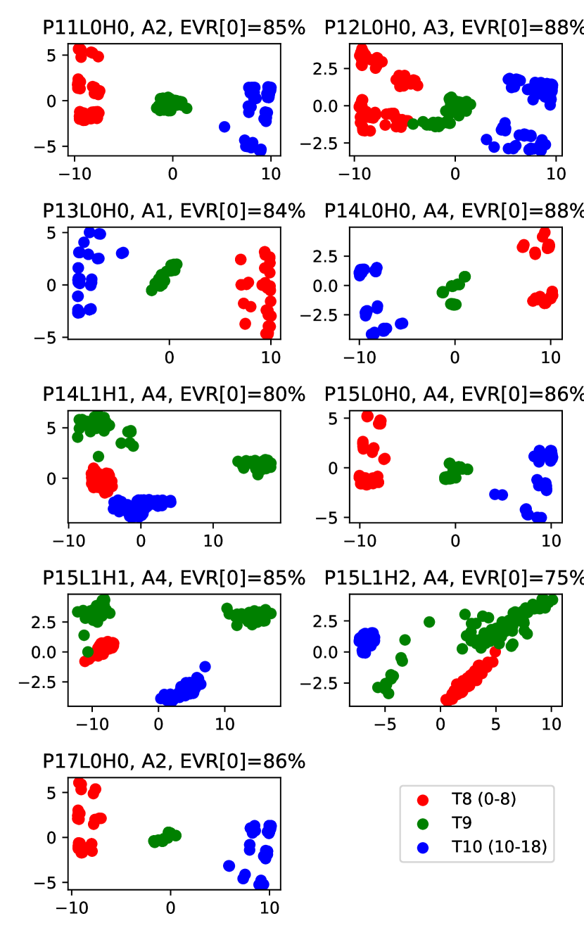
Figure 18: For 9 attention heads, for exactly 1 answer digit $A_{n}$each, PCA shows these interpretable results for the 6-digit Addition model. The 3 dot colours show the TriCase value of each question. The PCA data and TriCase quanta are both tri-state and strongly correlated.

Appendix J Appendix: Six-Digit Subtraction

Integer subtraction (e.g. 654321-789012=-0134691) and integer addition have similarities. Subtraction is conceptually more complex than integer addition. While $a+b$ and $b+a$ give the same answer, generally $a-b$ and $b-a$ give difference answers. In human subtraction the algorithm used to calculate $a-b$ changes depending on whether $a>b$ or $a<b$.

In our transformer-based models, Subtraction and Addition have some similar quanta. For example:

• In addition, the first answer digit is always and “1” or “0” and this token is the hardest to calculate accurately because of the “cascading carry 1” edge case. In subtraction, the first answer token is always “+” or “-” and this token is the hardest to calculate accurately because of the “cascading borrow 1” edge case.

• If $a>b$ then the algorithm to calculate $a-b$ and $a+b$ have strong structural similarities, allowing per-digit calculations with one sub-task moving data between digits (“carry 1” or “borrow 1”)

• If $a<b$ then the algorithm to calculate $a-b$ can use the mathematical identity that $1a-b=-(b-a)$. Our intuition is that the model will calculate if $a<b$, and if so will reuse the $a>b$ circuit, then negate the answer.

We created a very-low-loss 6-digit addition model. Figure 8 shows the lowest quanta impacted when ablating each node. We created a “mixed operations” model (6-digit, 3-layer, 4-head) to do both Addition and Subtraction. We initialised the untrained model with the addition model and trained it (with 80% subtraction and 20% addition questions) to be very low loss. This mixed model can predict one million addition and one million subtraction questions without error.

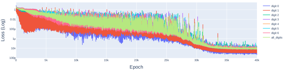
Figure 19: The per-digit log-loss curves for a 6-digit 3-layer 4-head mixed model trained to perform subtraction and addition after being initialised with a very low loss addition model.

To investigate what classes of questions the model is always getting wrong, we expanded our existing addition-specific metrics, to include subtraction-specific question categorisations (see Sec. 4.3. Figures 9 and  10 maps these quanta against nodes showing which are used for addition and subtraction.

The model contains a new sub-task that stands out: The algorithm relies on calculations done at token position P0, when the model has only seen one question token! What information can the model gather from just the first token? Intuitively, if the first token is a “8” or “9” then the first answer token is more likely to be a “+” (and not a “-”). The model uses this heuristic even though this probabilistic information is sometimes incorrect and so will work against the model achieving very low loss.

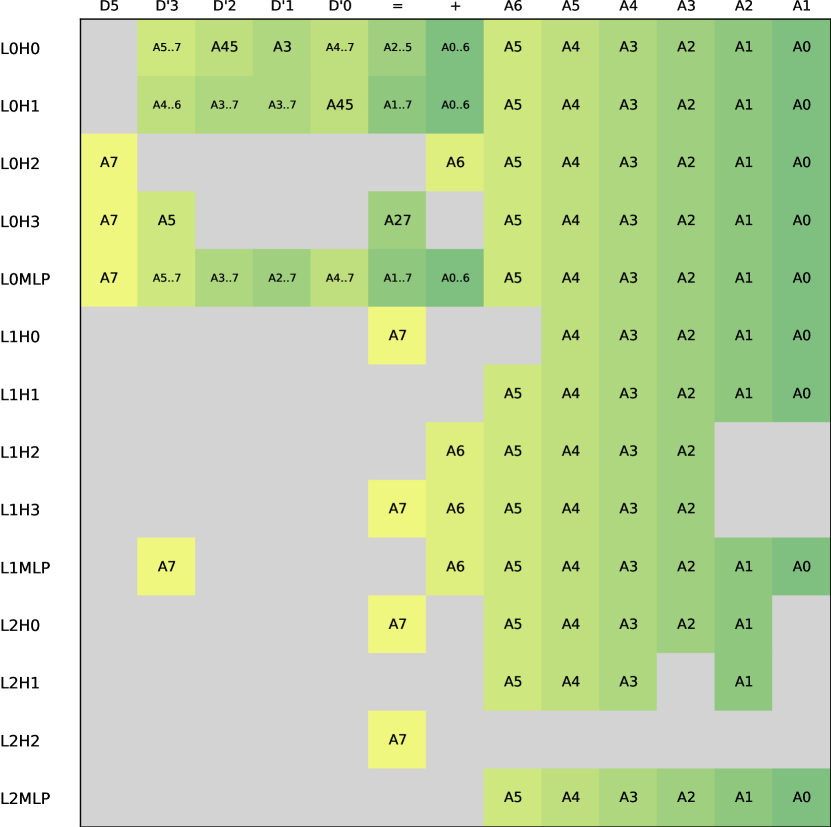
Figure 20: This map shows the answer digit(s) A0 .. A7 impacted when we ablate each useful node in the 6-digit 3-layer 4-head mixed model. A7 is the sign of the answer and calculated first. Note the similarity to the 5 and 6-addition Figures 7 and  17.

References

- Barak et al. (2022) Barak, B., Edelman, B. L., Goel, S., Kakade, S. M., Malach, E., and Zhang, C. Hidden progress in deep learning: Sgd learns parities near the computational limit. ArXiv, abs/2207.08799, 2022. URL https://api.semanticscholar.org/CorpusID:250627142.
- Cunningham et al. (2023) Cunningham, H., Ewart, A., Riggs, L., Huben, R., and Sharkey, L. Sparse autoencoders find highly interpretable features in language models, 2023.
- Elhage et al. (2021a) Elhage, N., Nanda, N., Olsson, C., Henighan, T., Joseph, N., Mann, B., Askell, A., Bai, Y., Chen, A., Conerly, T., DasSarma, N., Drain, D., Ganguli, D., Hatfield-Dodds, Z., Hernandez, D., Jones, A., Kernion, J., Lovitt, L., Ndousse, K., Amodei, D., Brown, T., Clark, J., Kaplan, J., McCandlish, S., and Olah, C. A mathematical framework for transformer circuits. Transformer Circuits Thread, 2021a. https://transformer-circuits.pub/2021/framework/index.html.
- Elhage et al. (2021b) Elhage, N., Nanda, N., Olsson, C., et al. A mathematical framework for transformer circuits. https://transformer-circuits.pub/2021/framework/index.html, 2021b.
- Geva et al. (2022) Geva, M., Caciularu, A., Wang, K. R., and Goldberg, Y. Transformer feed-forward layers build predictions by promoting concepts in the vocabulary space, 2022.
- Hendrycks & Mazeika (2022) Hendrycks, D. and Mazeika, M. X-risk analysis for ai research. ArXiv, abs/2206.05862, 2022. URL https://api.semanticscholar.org/CorpusID:249626439.
- Hendrycks et al. (2021) Hendrycks, D., Burns, C., Kadavath, S., Arora, A., Basart, S., Tang, E., Song, D., and Steinhardt, J. Measuring mathematical problem solving with the math dataset. In Thirty-fifth Conference on Neural Information Processing Systems Datasets and Benchmarks Track (Round 2), 2021.
- Hu et al. (2021) Hu, E. J., Shen, Y., Wallis, P., Allen-Zhu, Z., Li, Y., Wang, S., Wang, L., and Chen, W. Lora: Low-rank adaptation of large language models, 2021.
- Jenner et al. (2023) Jenner, E., Garriga-alonso, A., and Zverev, E. A comparison of causal scrubbing, causal abstractions, and related methods. https://www.lesswrong.com/posts/uLMWMeBG3ruoBRhMW/a-comparison-of-causal-scrubbing-causal-abstractions-and, 2023.
- Kruthoff (2024) Kruthoff, J. Carrying over algorithm in transformers, 2024.
- Liu & Low (2023) Liu, T. and Low, B. K. H. Goat: Fine-tuned llama outperforms gpt-4 on arithmetic tasks, 2023.
- Michaud et al. (2023) Michaud, E. J., Liu, Z., Girit, U., and Tegmark, M. The quantization model of neural scaling, 2023.
- Nanda (2023) Nanda, N. One layer sparce autoencoder. https://github.com/neelnanda-io/1L-Sparse-Autoencoder, 2023.
- Nanda et al. (2023) Nanda, N., Chan, L., Lieberum, T., Smith, J., and Steinhardt, J. Progress measures for grokking via mechanistic interpretability, 2023.
- nostalgebraist (2020) nostalgebraist. interpreting gpt: the logit lens. https://www.alignmentforum.org/posts/AcKRB8wDpdaN6v6ru/interpreting-gpt-the-logit-lens, 2020.
- Olah et al. (2020) Olah, C., Cammarata, N., Schubert, L., Goh, G., Petrov, M., and Carter, S. Zoom in: An introduction to circuits. Distill, 2020. doi: 10.23915/distill.00024.001. https://distill.pub/2020/circuits/zoom-in.
- Quirke & Barez (2024) Quirke, P. and Barez, F. Understanding addition in transformers. In The Twelfth International Conference on Learning Representations, 2024. URL https://arxiv.org/pdf/2310.13121.pdf.
- Raukur et al. (2022) Raukur, T., Ho, A. C., Casper, S., and Hadfield-Menell, D. Toward transparent ai: A survey on interpreting the inner structures of deep neural networks. 2023 IEEE Conference on Secure and Trustworthy Machine Learning (SaTML), pp. 464–483, 2022. URL https://api.semanticscholar.org/CorpusID:251104722.
- Schaeffer et al. (2023) Schaeffer, R., Miranda, B., and Koyejo, S. Are emergent abilities of large language models a mirage?, 2023.
- Stolfo et al. (2023) Stolfo, A., Belinkov, Y., and Sachan, M. A mechanistic interpretation of arithmetic reasoning in language models using causal mediation analysis. In Proceedings of the 2023 Conference on Empirical Methods in Natural Language Processing, pp. 7035–7052, 2023.
- Voita et al. (2023) Voita, E., Ferrando, J., and Nalmpantis, C. Neurons in large language models: Dead, n-gram, positional, 2023.
- Zhang et al. (2022) Zhang, A., Xing, L., Zou, J., and Wu, J. C. Shifting machine learning for healthcare from development to deployment and from models to data. Nature Biomedical Engineering, 6:1330 – 1345, 2022. URL https://api.semanticscholar.org/CorpusID:250283181.
Acknowledgements
The authors would like to thank Apart Labs (https://apartresearch.com/lab) for their support in producing this paper and more generally supporting the entry of people new to AI Safety into the field.