Minute-Cadence Observations of the LAMOST Fields with the TMTS: V. Machine Learning Classification of TMTS Catalogues of Periodic Variable Stars

Abstract

Periodic variables are always of great scientific interest in astrophysics. Thanks to the rapid advancement of modern large-scale time-domain surveys, the number of reported variable stars has experienced substantial growth for several decades, which significantly deepened our comprehension of stellar structure and binary evolution. The Tsinghua University–Ma Huateng Telescopes for Survey (TMTS) has started to monitor the LAMOST sky areas since 2020, with a cadence of 1 minute. During the period from 2020 to 2022, this survey has resulted in densely sampled light curves for ~30,000 variables of the maximum powers in the Lomb-Scargle periodogram above the 5$\sigma$ threshold. In this paper, we classified 11,638 variable stars into 6 main types using XGBoost and Random Forest classifiers with accuracies of 98.83% and 98.73%, respectively. Among them, 5301 (45.55%) variables are newly discovered, primarily consisting of $\delta$ Scuti stars, demonstrating the capability of TMTS in searching for short-period variables. We cross-matched the catalogue with $Gaia$’s second Data Release (DR2) and LAMOST’s seventh Data Release (DR7) to obtain important physical parameters of the variables. We identified 5504 $\delta$ Scuti stars (including 4876 typical $\delta$ Scuti stars and 628 high-amplitude $\delta$ Scuti stars), 5899 eclipsing binaries (including EA-, EB- and EW-type) and 226 candidates of RS Canum Venaticorum. Leveraging the metal abundance data provided by LAMOST and the Galactic latitude, we discovered 8 candidates of SX Phe stars within the class of "$\delta$ Scuti stars". Moreover, with the help of $Gaia$ color-magnitude diagram, we identified 9 ZZ ceti stars.

1 Introduction

Figure 1: Sky map (in equatorial coordinates) of TMTS uninterrupted observations during 2020-2022. The color displays the maximum number of uninterrupted exposures within a single night, as in TMTS-II. We used the HEALPIX package (http://healpix.sourceforge.net) with NSIDE=128 to plot this sky map (Gorski et al., 2005).

Since ancient times, people have been fascinated by changes occurring in the night sky. Large-scale surveys play a crucial role in the study of variables in the modern era. Over the past decade, missions like the All-Sky Automated Survey for Supernovae (ASAS-SN, Jayasinghe et al. 2019), the Catalina Sky Survey (CSS, Drake et al. 2014), the Asteroid Terrestrial-impact Last Alert System (ATLAS, Heinze et al. 2018) among others offer unique opportunities to explore variable stars. The $Gaia$ DR2 provides a detailed catalogue of more than 1 million variable stars, including ~228 thousand RR Lyrae stars, ~151 thousand long-period variable stars (LPVs), ~147 thousand rotational variables, etc (Brown et al., 2018; Holl et al., 2018). $Gaia$ $G$, $G$_BP and $G$_RP integrated photometric band measurements as well as parallaxes with unprecedented accuracy substantially help to locate stars in the $Gaia$ color-magnitude diagram (CMD), which facilitates classification and further studies of stellar evolution history. The Optical Gravitational Lensing Experiment (OGLE) sky survey has started sky monitoring for more than 30 years. Initially designed as hunter for gravitational microlensing events and dark matter, the OGLE has obtained photometric datasets for millions of variables in the Galactic bulge, Galactic disk and the Magellanic Clouds (Udalski et al., 2015). In the foreseeable future, the Large Synoptic Survey Telescope (LSST, Ivezić et al. 2019) may discover billions of variable stars, potentially ushering in a transformative era in the field of astronomy. However, due to the long sampling cadences (e.g. $\geq$ 1 day), previous large-scale surveys are constrained in their ability to identify short-period variables. The advent of high-cadence surveys, such as the ZTF high-cadence Galactic Plane Survey with a cadence of 40 sec (Kupfer et al., 2021), has brought groundbreaking opportunities to the identification of variables with periods below several hours, such as ultra-compact binaries (UCBs) and compact pulsators.

Study of variable stars is an essential part in time-domain astronomy, which focuses on transients and violent outbursts in the universe. Pulsating stars are a vital category among variable stars. Situated within the instability strip, pulsating stars mainly consist of Cepheids, $\delta$ Scuti stars, RR Lyrae stars, ZZ Ceti stars and LPVs. Mainly triggered by the $\kappa$ mechanism, these pulsators follow period-luminosity ($P-L$) relations, among which the well-defined $P-L$ relations of Cepheids (Leavitt & Pickering, 1912) rendering them invaluable for measuring cosmic distances and aiding in the determination of the Hubble constant (Sandage et al., 2006; Riess et al., 2018). In the big family of pulsating variables, stars manifest significant discrepancies in their periods. $\delta$ Scuti stars are a subclass of pulsating stars which undergo multi-mode pulsations (Breger, 2000) with periods below 0.3 d. This bound is somewhat arbitrarily set to distinct them from classical pulsators such as RR Lyrae stars and Cepheids. Pre-main-sequence A-type stars are the fastest known $\delta$ Scuti pulsators (Holdsworth et al., 2014), among which HD 34282 has the shortest period ($P$ = 18.12 min) ever observed (Rodríguez, 2004). The study of $\delta$ Scuti stars would answer some long-standing questions in stellar physics, such as the pulsator fraction within the $\delta$ Scuti instability strip as well as the determination of the edges of the instability strip (Murphy et al., 2019). On the other hand, the periods of Cepheids are usually a few days. For LPVs like mira variables which are characterized by very red colors, periods can extend to hundreds or even thousands of days (Iwanek et al., 2022). This vast disparity in periods reflects the abundance and diverse nature of pulsating stars.

Eclipsing binaries are another important subclass of transients discovered by wide-field survey projects. Binaries play a crucial role in understanding stellar evolution history (e.g. common envelope evolution, mass exchange and stellar winds, Taam & Sandquist 2000; Plavec 1968; Theuns & Jorissen 1993). In addition, they could be progenitor of Type Ia Supernovae (Rebassa-Mansergas et al., 2019), which is of significant importance in cosmology. Periods of binaries range from several hours to a few days, while short-period binaries have been getting increasing attention recently, since the mergings of UCBs, whose period are typically less than an hour (Chen et al., 2020b), are the most prominent gravitational wave source (Postnov & Yungelson, 2014). Observed by the LIGO-Virgo detector network, the gravitation-wave signal GW170817 is explained as a binary neutron star merger, while GW190814 is generated by a compact binary coalescence involving a black hole and a compact object (Abbott et al., 2017, 2020). Several short-period eclipsing binaries, such as the AM CVn stars SDSS J0926+3624 ($P$ = 28 min, Copperwheat et al. 2011), the double-white-dwarf binary SDSS J0651+2844 ($P$ = 12.75 min, Brown et al. 2011) and ZTF J1539+5027 ($P$ = 6.91 min, Burdge et al. 2019), have periods considerably shorter than the 0.22 day short-period limit of contact eclipsing binaries (Rucinski, 1992), posing a new challenge to this short-period limit.

In the past decade, machine learning technique becomes increasingly prevalent in astronomy, with the astronomical data underwent exponential expansion, (e.g., Richards et al. 2011; Bloom et al. 2012; Kim & Bailer-Jones 2016; Naul et al. 2018; Hosenie et al. 2020). Holding great potential to enhance our interpretation of vast and complex data, machine learning algorithms effectively resolve regression, classification, clustering and dimension reduction problems. In practice, machine learning techniques show particular promising in tackling intriguing problems such as galaxy identification (Krakowski et al., 2016), variable star classification (Jayasinghe et al., 2019; Chen et al., 2020a) and exoplanet exploration (Nixon & Madhusudhan, 2020).

The Tsinghua University–Ma Huateng Telescopes for Survey (TMTS), consisting of four optical telescopes, is located at the Xinglong Station of NAOC. TMTS has a field of view (FoV) up to 18 deg² (Zhang et al., 2020), covering a wavelengths range from 400 to 900 mm. For an exposure time of 60s, TMTS can reach ~19.4 mag in white light (or Luminous filter) at 3$\sigma$ detection limit. To ensure the quality of our analysis, we only picked the light curves (LCs) with at least 100 uninterrupted measurements (Lin et al. 2022, hereafter TMTS-I). TMTS has already yielded progress in several aspects, including the identification of over 1000 short-period variables (i.e., $P$ < 2 hr, Lin et al. 2023c, hereafter TMTS-II), the record of 125 flare stars (Liu et al., 2023), the discoveries of a 18.9-min blue large-amplitude pulsators (BLAPs, Lin et al. 2023b) and a 20.5-min sdB binary (Lin et al., 2023a). In this paper, we search for periodic variables ($P$ < 7.5 hr) using two advanced algorithms (XGBoost and Random Forest) in the TMTS Catalog of Periodic Variable Stars. Observations and data are introduced in Section 2, and the method and result of the classification are discussed in Section 3. Section 4 explains the characteristics of the catalogues. We discuss the overall catalogue and each type of variables in detail in Section 5. A summary of our work is given in Section 6.

2 Data

Since 2020, TMTS has monitored 449 LAMOST/TMTS plates by the end of 2022, covering a total of 6977 deg² of the sky, which are shown in Figure 1. This effort leads to the production of 19,099,266 uninterrupted LCs with more than 100 epochs. We adopted the Lomb-Scargle periodogram (LSP; Lomb 1976; Scargle 1982) to analyze these LCs. Using the distribution of modified false-alarm probability (FAP) as adopted in papers of TMTS-I and -II, we calculated the maximum powers in LSP (hereafter $LSP\mathrm{{}_{max}}$) and determined the 5$\sigma$ and 10$\sigma$ thresholds for each source. Among the millions of sources detected, the numbers of those with $LSP\mathrm{{}_{max}}$ $>$ 5$\sigma$ and $>$ 10$\sigma$ thresholds are $>$ 30000 and $>$ 8000, respectively. The TMTS LCs are cross-matched with $Gaia$ DR2 (the pipeline system of TMTS cross-matched DR2) and LAMOST DR7 to obtain some crucial photometric and spectroscopic parameters, such as dereddening color $(B\mathrm{{}_{p}}-R\mathrm{{}_{p}})_{0}$, effective temperature $T$_eff and spectral type. We derived the G-band absolute magnitude ($G$_abs) of variables with reliable parallax (i.e., $\varpi/\sigma_{\varpi}\geq 5.0$) as in paper TMTS-II.

To ensure the accuracy of our classifications of the TMTS periodic variables, we first cross-matched the TMTS LCs with the variable sources of the International Variable Star Index (VSX, Watson et al. 2006), which is a database providing comprehensive information of over 2200,000 known and suspected variable stars. This cross match indicates that 6801 sources have been recorded and identified by the VSX. To augment the dataset, a manual examination was conducted, resulting in another 1015 sources with assigned classifications. Among the ($6801+1015=$) 7816 identified sources, 6146 have $LSP\mathrm{{}_{max}}$ above the 10$\sigma$ threshold.

We visually inspected all the LCs of the 6146 sources and excluded some low-quality (low SNR ratio, i.e. SNR $<$ 20) LCs. It is worth noting that classifying a variable star based solely on the information extracted from the LCs can be challenging. Incorporating supplementary information, especially color and absolute magnitude, can significantly enhance the reliability of classification. The $Gaia$ color-magnitude diagram (CMD), a close counterpart to the Hertzsprung–Russell diagram, is a useful tool for the classification, as it enables the segregation of variables into distinct regions based on their characteristics (Eyer et al., 2019). For instance, $\delta$ Scuti stars locate in the instability strips, while eclipsing binaries can appear anywhere in the CMD.

Considering the importance of $Gaia$ $(B\mathrm{{}_{p}}-R\mathrm{{}_{p}})_{0}$ and $G$_abs, we exclusively deemed the classification of sources with these information to be reliable. A total of 4506 sources were finally selected as the labelled dataset (hereafter Dataset-I), which serves as the training set and test set to train the classifiers and evaluate their performances. Dataset-I contains 1120 typical $\delta$ Scuti stars (DSCT), 256 high-amplitude $\delta$ Scuti stars (HADS), 49 RS Canum Venaticorum (RS), and 3081 eclipsing binaries. The eclisping bianries includes 2985 W UMa type (EW), 42 Algol type (EA) and 54 $\beta$ Lyr type (EB). “DSCT” refers to typical $\delta$ Scuti stars which include subtypes of DSCT, DSCTc (obsolete VSX type designation, low-amplitude $\delta$ Scuti stars with V-band light amplitude $<$ 0.1 mag) and DSCTr (VSX type designation, a subtype of $\delta$ Scuti stars in ASAS-3). SX Phe variables are metal-poor pulsating sub-dwarfs which resemble $\delta$ Scuti stars phenomenologically. As SX Phe variables can hardly be identified through LCs, they are included in the class “DSCT” as well (Soszyński et al., 2021). We will discuss candidates of SX Phe variables using the metal abundance data provided by LAMOST and the Galactic latitude in Section 4. We use “HADS” to represent HADS and HADS(B) (VSX type designation, first/second overtone double-mode HADS). The criteria that distinguish HADS from DSCT is that the former light-variation amplitude exceeds 0.3 mag in the $V$ band. While this threshold may appear somewhat discretionary, HADS and DSCT exhibit divergent characteristics in light of the LC shapes, rotation speed, evolutionary stages and so on (Chang et al. 2013; Chen et al. 2020a; McNamara 2011). We therefore regard them as two distinct groups. To avoid ambiguity, we use “$\delta$ Scuti stars” to encompass the entire category (including typical $\delta$ Scuti stars and high-amplitude $\delta$ Scuti stars), while “DSCT” is used to denote typical $\delta$ Scuti stars and “HADS” specifically designates high-amplitude $\delta$ Scuti stars. The sample sizes for other types are insufficient (i.e., number $<$ 30) to establish datasets with adequate statistical robustness without risking overfitting, even with carefully-designed over-sampling algorithms. This overfitting could arise from that the models misinterprete the specific characteristics of individual light curves as general traits of the entire class. In the future, we intend to employ novelty detection algorithms for the identification of such variables.

We randomly checked 300 unlabeled LCs, finding a relatively low false-positive rate in the 10$\sigma$ threshold LCs. However, over 70% of the 5$\sigma$ threshold LCs were recognized to be non-astrophysically variable sources, as a typical concern in high-cadence surveys (Kupfer et al., 2021). We thus retained all the 10$\sigma$ threshold LCs, while applying an additional minimum threshold of $LSP\mathrm{{}_{max}}$ = 30 for the 5$\sigma$ threshold LCs. This selection process yields ~8000 unlabeled LCs, referred to as Dataset-II.

Dataset-I and II only include limited kinds of variables due to the observation strategy of TMTS (see paper TMTS-I). The upper period bound of TMTS is ~7.5 h, preventing us from discovering variables with longer periods, such as Cepheids and LPVs. In fact, the longest period detected in Dataset-I and -II is 6.21 h. Periods of Cepheids are typically above 1 d, far exceeding the upper period limit of TMTS. RR Lyrae stars are another frequently observed stars with periods of 0.2–1.0 d. A considerable portion of RRc variables having periods below 0.3 d (7.2 h), falls within the detection range of TMTS. However, they are old and commonly present in globular clusters located around the Galactic core (Soszynski et al., 2014), which is not covered by TMTS, resulting in their scarcity in our catalogue.

3 Classification

3.1 Method

Table 1: Features of the XGBoost and RF classifier.

Feature	Description	Reference
Period	Photometric period determined through the Lomb–Scargle periodogram.
$(B\mathrm{{}_{P}}-R\mathrm{{}_{P}})_{0}$	$(G$BP-$G$$\mathrm{{}_{RP}})_{0}$, dereddened color provided by $Gaia$ DR2.
$M\mathrm{{}_{G}}$	G-band (330 nm to 1050 nm) absolute magnitude provided by $Gaia$ DR2.
Amplitude	Peak-to-peak amplitude obtained from the fourth-order Fourier fitting of the LCs.
Cusum	The range of the cumulative sum of the LCs. Cusums of LCs with longer-term variability are usually larger.	Kim et al. (2014)
Eta	Measures the degree of trends in a long-term baseline, which is useful in separate variables with different periods.	Kim et al. (2014)
Hl_amp_ratio	Ratio between higher and lower amplitude than average. Hl_amp_ratios for EAs are higher by definition.	Kim & Bailer-Jones (2016)
Kurtosis	The fourth standardized moment of the distribution, measuring the tailedness of the distribution. Kurtosis=$\frac{\frac{1}{n}\sum_{i=1}^{n}(x_{i}-\bar{x})^{4}}{(\frac{1}{n}\sum_{i=1}^{n}(x_{i}-\bar{x})^{2})^{2}}-3$
Quartile31	Difference between 75% percentile and 25% percentile of the LCs.	Kim & Bailer-Jones (2016)
Shapiro_w	Shapiro-Wilk test for normalization.	Kim & Bailer-Jones (2016)
Skewness	The third standardized moment of the distribution, measuring its asymmetry. Skewness=$\frac{\frac{1}{n}\sum_{i=1}^{n}(x_{i}-\bar{x})^{3}}{(\frac{1}{n}\sum_{i=1}^{n}(x_{i}-\bar{x})^{2})^{3}/2}$
Stetson_k	Stetson K index, describing the shape of the LCs.	Kim et al. (2014)
Weighted_mean	Weighted mean of the LCs, the weight of each data point in the LCs is inversely proportional to its measurement error, which assigns higher weights to data points with smaller errors.
Weighted_std	Weighted standard deviation of the LCs.
Phase_eta	Eta for phase-folded LCs.	Kim et al. (2014)
Phase_cusum	Cusum for phase-folded LCs.	Kim et al. (2014)
Slope_per10	10% percentile of slopes of a phase-folded LC.	Long et al. (2012)
Slope_per90	90% percentile of slopes of a phase-folded LC.	Long et al. (2012)
R21	$a_{2}$ / $a_{1}$, 2nd to 1st amplitude ratio obtained from the fourth-order Fourier fitting.
R31	$a_{3}$ / $a_{1}$, 3nd to 1st amplitude ratio obtained from the fourth-order Fourier fitting.
R41	$a_{4}$ / $a_{1}$, 4nd to 1st amplitude ratio obtained from the fourth-order Fourier fitting.
$\Phi$21	$\Phi_{2}$ - 2$\Phi_{1}$, the phase difference between 2nd and 1st phase obtained from the fourth-order Fourier fitting.
$\Phi$31	$\Phi_{2}$ - 3$\Phi_{1}$, the phase difference between 3rd and 1st phase obtained from the fourth-order Fourier fitting.

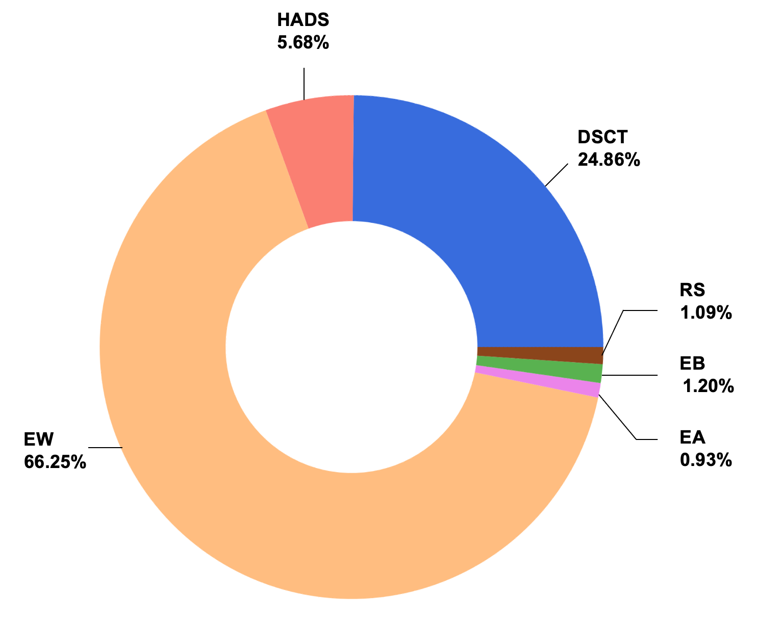
Figure 2: Pie chart of the distribution of variable stars within Dataset-I, which is heavily imbalanced. EWs account for 66.25%, while EAs comprise a mere 0.93%, underscores the pronounced disparity of over 70-fold between these two groups.

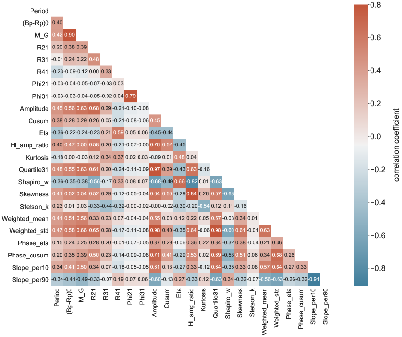
Figure 3: Correlation matrix of the features used in classification. The color of each square represents the value of the Pearson correlation coefficient between the corresponding features. A predominantly white color indicates a minimal correlation between a pair of features. Conversely, a thicker red (blue) color indicates a stronger positive (negative) correlation between the features.

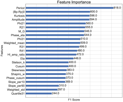
Figure 4: Feature importance of the feature set of the XGB classifier. The x-axis shows the F₁ scores (represents the gain) of each feature, and the y-axis displays the names of the features.

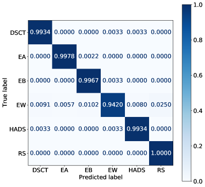
Figure 5: The normalized confusion matrix derived from the XGB classifier (left) and the RF classifier (right) based on the labelled dataset (Dataset-I). The x-axis represents the prediction class obtained from the classifier, and the y-axis displays the true group of a variable star.

In pursuit of higher prediction accuracy, we trained two classifiers, the XGBoost (XGB) classifier and the Random Forest (RF) classifier. Both classifiers would undergo training and testing in Dataset-I, and then predict the classes of each LCs in Dataset-II as well as providing a probability of the classification (Chen et al., 2015; Breiman, 2001). XGBoost and random forest are two popular machine learning algorithms based on ensemble learning techniques, where multiple decision trees are integrated to generate predictions, constructing a powerful knowledge discovery and data mining model (Dong et al., 2020). Both algorithms can be paralleled to speed up the training process and are robust to over-fitting. However, there are still certain differences between them. Random forest creates multiple weak decision trees independently, aggregating the predictions given by each tree to reach the ultimate result. XGBoost, using gradient boosting, optimizes the loss function by iteratively adding new trees. Comparing with neural networks (NNs), the two algorithms are more interpretable and require less preprocessing of the data. For instance, NNs exhibit sensitivity to the initial phases of LCs, which are external to the variability. Consequently, preprocessing steps or structural adjustments of the neural network are necessary (Zhang & Bloom, 2021). Moreover, XGBoost and random forest algorithms can provide insight into the importance of each feature input, allowing us to identify the key characteristics of the LCs to help distinguish different types. Although NNs may work better in large and complex datasets (Bishop, 1994), the capabilities of our classifiers are sufficient for the study.

Dataset-I is extremely imbalanced, as illustrated in Figure 2, where the number of EWs is more than 70 times that of the least abundant EAs. Considering eclipsing binaries alone, VSX recorded 812 EAs, 121 EBs and 62,356 EWs with periods below 7.5 h, roughly consistent with the proportion of these variables in Dataset-I. Due to the small numbers of some classes and the modest size of Dataset-I, it is hard to build a balanced training set. Although XGBoost and Random Forest algorithms can handle imbalanced datasets, the result without any preprocessing was not satisfactory. So we used Synthetic Minority Oversampling Technique (SMOTE, Chawla et al. 2002), an over-sampling technique, to prepare for a balanced training set. Based on the K-Nearest Neighbors algorithm, SMOTE synthesizes new instances for the minority classes by interpolating between existing samples from these classes, effectively increasing their representation.

We extracted some basic features (i.e.,features not related to period and the light curve fitting) of the LCs with the help of the UPSILoN package (Kim & Bailer-Jones, 2016). We simply used the “extract_features” module instead of its classification algorithm. Due to the importance of period determination, we carefully calculated it through LSP (see also paper TMTS-II) and fit the LCs with a fourth-order Fourier function (Chen et al., 2020a):

$$f=a_{0}+\sum_{i=1}^{4}a_{i}\cos(2\pi it/P+\phi_{i})$$ (1)

where $a_{i}$ (i = 0,1,2,3,4) and $\phi_{i}$ (i = 1,2,3,4) represent the Fourier amplitudes and phases in each order. Notice that we used a fourth-order fitting, while UPSILoN chooses a third-order function. We studied the residual of the third-order fitting, finding that nearly half of the residuals exceed the error of the magnitude. On the contrary, the fourth-order fitting leads to only 7.4% of the residuals above the magnitude error. Then we calculated some critical parameters like $R$₂₁ and $\Phi$₂₁ based on the fitting. Considering the challenge of classifying variable stars based on LCs alone, we included $Gaia$ $(B\mathrm{{}_{p}}-R\mathrm{{}_{p}})_{0}$ and $G$_abs into the feature list. Since only a small fraction of the sources in Dataset-I and II have LAMOST log $g$, $T$_eff and spectral type, we did not select these features. The complete set of features and their explanations in both classifiers are summarized in Table 1.

Features that exhibit low correlations are generally preferred in machine learning classification, as they are more likely to provide independent information, thereby contributing to the model’s ability to generalize and improve the classification accuracy. However, correlated features also have positive impacts. They enhance the stability of the algorithms by offering complementary information, and reduce the risk of overfitting by preventing the algorithms from relying excessively on an individual feature. Commonly, a correlation coefficient $r$ above 0.8 or below -0.8 would be considered a strong correlation. According to this criterion, as illustrated in Figure 3, most of the features in our feature set exhibit weak or moderate correlations. However, strong correlations exist between certain features. For example, $G$_abs and $(B\mathrm{{}_{p}}-R\mathrm{{}_{p}})_{0}$ show a positive correlation with $r$ = 0.9, because of the distribution pattern in the CMD. Similarly, quartile₃₁, weighted_std and amplitude show a strong correlation, because they represent different measurements of LC variabilities. Shapiro_w and hl_amp_ratio exhibit a noticeable negative correlation with r = $-$0.82. This relationship can be readily comprehended, as shapiro_w measures the extent to which a distribution deviates from a normal distribution. Larger deviations (as those found in the LCs of EAs) tend to result in an increase in hl_amp_ratio (a ratio between higher and lower amplitude relative to the average).

Figure 4 shows the importance of all features used in our classification, where the importance is represented by a parameter named as F₁ score. The more a feature contributes to the improvement of classification accuracy, the greater its gain and therefore its F₁ score. Among various features, the most important one is the period, highlighting the critical role of precise period determination. Features that characterize the shape of the LCs from different aspects, such as kurtosis, amplitude and R₂₁, are of significant importance. Additionally, in accordance with our predictions, $Gaia$ $G$_abs and $(B\mathrm{{}_{p}}-R\mathrm{{}_{p}})_{0}$ also have great effects on the classifications.

3.2 Accuracy

Table 2: The precision, recall and F₁ scores of the XGB classifier.

Type	Precision	Recall	F1 score
DSCT	0.9956	0.9890	0.9923
EA	1.0000	0.9945	0.9972
EB	0.9989	0.9903	0.9946
EW	0.9420	0.9916	0.9662
HADS	0.9923	0.9912	0.9917
RS	1.0000	0.9729	0.9863
Macro-average	0.9881	0.9883	0.9881
Weighted-average	0.9887	0.9883	0.9884

Table 3: The precision, recall and F₁ scores of the RF classifier.

Type	Precision	Recall	F1 score
DSCT	0.9934	0.9879	0.9907
EA	0.9978	0.9944	0.9961
EB	0.9967	0.9882	0.9924
EW	0.9420	0.9893	0.9651
HADS	0.9934	0.9890	0.9912
RS	1.0000	0.9751	0.9874
Macro-average	0.9872	0.9873	0.9871
Weighted-average	0.9878	0.9873	0.9874

Three scores are used to evaluate the performance of the classifiers. Precision measures the fraction of true positives relative to the predicted positive instances:

$$\mathrm{Precision=\frac{True\ Positives}{True\ Positives+False\ Positives}}.$$ (2)

Recall refers to the proportion of true positives among actual positive instances:

$$\mathrm{Recall=\frac{True\ Positives}{True\ Positives+False\ Negatives}}.$$ (3)

Where the true positives refer to the samples correctly classified as belonging to a specific class, while false positives indicate samples that do not belong to this class but are incorrectly classified as part of it. Moreover, false negatives represent the samples that actually belong to that class but are incorrectly classified as not belonging. A clear trade-off exists between these two measurements. Aiming to improve precision, the algorithm tends to minimize predicting positive samples to mitigate false positives. On the contrary, for optimizing recall, the model is inclined to select more positive samples to avoid missing any possible positives. Thus, F₁ score is the harmonic mean of precision and recall, which provides a balanced measure of the algorithm’s performance:

$$\mathrm{F_{1}\ score=\frac{2}{1/precision+1/recall}}.$$ (4)

The normalized confusion matrices of both classifiers is shown in Figure 5. We used two measurements to evaluate the overall performance of the classifiers. Macro-average treats each class fairly, while weighted-average gives each type a weight that is proportional to the number of samples in that class. As our dataset is heavily imbalanced, weighted-average is more appropriate in measuring the performance of the classifiers. Some analogous patterns can be discerned in both confusion matrices. Both classifiers exhibit excellent performance in distinguishing EAs and RS CVn candidates, potentially owing to the distinctive shapes of their light curves. The overall performance of the XGB classifier is slightly better than the RF classifier. The macro-average and weighted-average F₁ scores of the XGB classifier are 98.81% and 98.84%, respectively. The precision, recall and F₁ scores for each type are summarized in Table 2. The F₁ scores for all six types are higher than 96%, which indicates that the variable stars are well distinguished by the XGB classifier. With F₁ scores $\geq$ 99%, the DSCT, EA, EB and HADS classes are very well classified, while the scores of EWs appear to be relatively diminished.

For the RF classifier, its performance is summarized in Table 3. All the F₁ scores are higher than 96%, with the macro-average and weighted-average F₁ scores of 98.71% and 98.74%. Similar to the situation of the XGB classifier, the EW class has lower F₁ scores than other classes. In both classifiers, the relatively lower F₁ scores of EWs may potentially attributed to the contamination of EBs and RS CVn candidates, as illustrated in Figure 5. EBs are semi-detached eclipsing binaries occupying an intermediate evolutionary state between EAs and EWs, and in some cases their LCs closely resemble those of EWs, leading to challenges in their differentiation. In fact, sometimes the classification of eclipsing binaries has been simplified to primarily two categories (Chen et al., 2020a): EA-type (detached) and EW-type (contact). Furthermore, some RS CVn variables are themselves eclipsing binaries, which explains the occasional similarity between their LCs and those of EWs.

In both classifiers, the F₁ score for DSCT, HADS, EA and EB exceeds 99%, while EW slightly lags behind at 96%. These results underscore the effectiveness of our feature selection and algorithm training processes. However, we shall point out that the confusion matrices and the scores are derived from Dataset-I (the labelled dataset), while Dataset-II (the unlabelled dataset) might contain fainter objects with noisier light curves, making them more susceptible to misclassification. As a consequence, the scores might be degraded in Dataset-II. Additionally, we acknowledge that our training and test datasets are relatively limited in size and may not yield the same level of accuracy if expanded.

When appling the classifiers to Dataset-II, we find that some objects do not belong to the 6 main classes explored in this paper. To avoid misclassifications, we conducted a comprehensive manual inspection of all sources, which should minimize the probability of such errors.

4 Catalogues

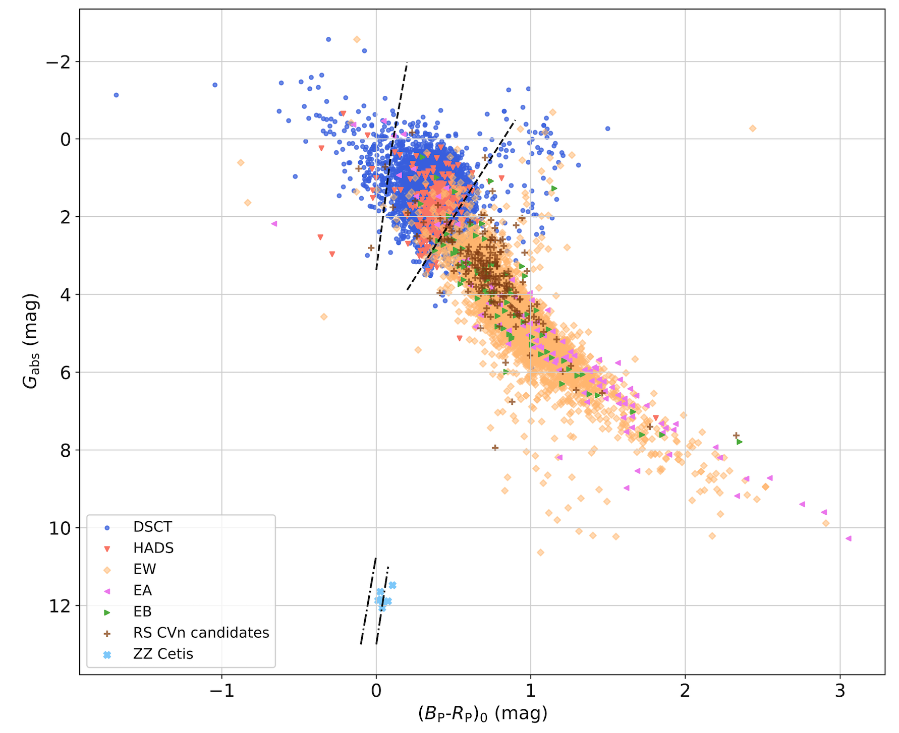
Figure 6: Distribution of variable stars in TMTS Catalog of Periodic Variable Stars across the color-magnitude diagram. Color-coded symbols represent different classes of variable stars, include typical $\delta$ Scuti stars (DSCT, royal blue), high amplitude $\delta$ Scuti stars (HADS, red), EW-type eclipsing binaries (EW, orange), EA-type eclipsing binaries (EA, pink), EB-type eclipsing binaries (EB, green), RS CVn candidates (RS, brown) and ZZ Ceti variables (ZZ, azure). The dashed lines and dash-dotted lines indicate the instability strip edges for $\delta$ Scuti stars (Murphy et al., 2019) and ZZ Ceti stars (Caiazzo et al., 2021), respectively. The edges of the instability strip are calculated by using the relationship of $Gaia$ $B_{\mathrm{P}}-R_{\mathrm{P}}$ and $T_{\mathrm{eff}}$ (see also Jordi et al. 2010).

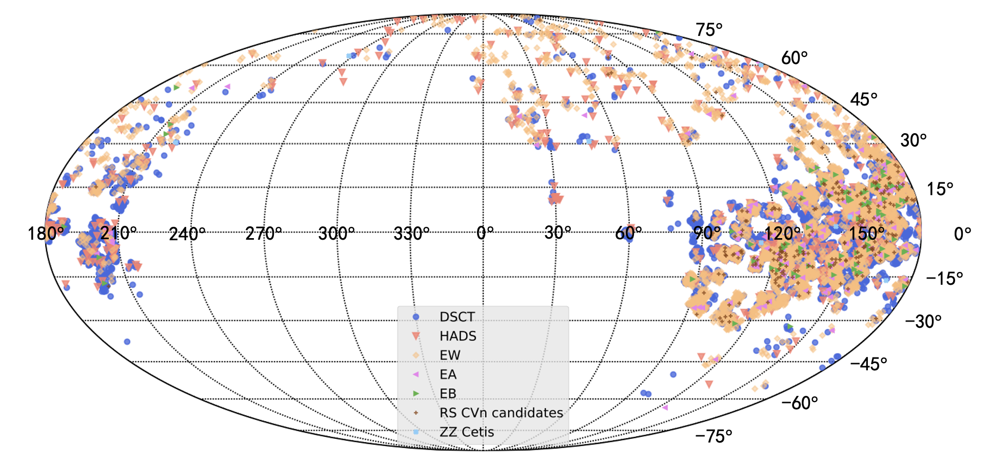
Figure 7: Distribution of variable stars in TMTS Catalog of Periodic Variable Stars in Galactic coordinates.

Table 4: All and newly discovered variables in TMTS Catalogues of Periodic Variable Stars.

Type	Total number	Newly discovered (Fraction)
DSCT	4876	4297 (88.13%)
EA	117	18 (15.38%)
EB	84	18 (21.43%)
EW	5698	780 (13.69%)
HADS	628	74 (11.78%)
RS CVn	226	108 (47.79%)
ZZ Ceti	9	6 (66.67%)

Table 5: Example catalogue for typical $\delta$ Scuti stars (DSCT) and high amplitude $\delta$ Scuti stars (HADS) in TMTS Catalogues of Periodic Variable Stars.

Type	source I.D.	R.A.	Dec.	Period	Amp	$R_{21}$	$\Phi_{21}$	$G\mathrm{{}_{abs}}$	$(B\mathrm{{}_{p}}-R\mathrm{{}_{p}})_{0}$	spec.type	VSX type	$T\mathrm{{}_{eff}}$	log g
		deg	deg	hours	mag			mag	mag			K	cm-2
HADS	TMTS J00000450+5146157	0.01875	51.77104	2.28702	0.077	0.464	0.435				DSCT
DSCT	TMTS J00001301+5520331	0.05422	55.34254	2.39646	0.018	0.028	0.701	1.086	0.412
DSCT	TMTS J00001318+5144112	0.05494	51.73646	1.64768	0.036	0.262	-0.180	2.428	0.356		DSCT
DSCT	TMTS J00003793+5423372	0.15805	54.39367	2.22930	0.033	0.384	0.584	1.206	0.375
DSCT	TMTS J00004133+6034008	0.17223	60.56690	0.74820	0.006	0.069	0.288	1.277	0.150
DSCT	TMTS J00004531+5857086	0.18880	58.95239	1.27363	0.010	0.113	0.108	1.494	0.345	F0	DSCT	7148.6	3.913
DSCT	TMTS J00004603+5649520	0.19179	56.83111	1.72859	0.012	0.179	1.436	1.978	0.406	F0		7329.5	3.951
DSCT	TMTS J00011153+5402497	0.29804	54.04713	0.86593	0.016	0.022	-0.003	1.565	0.271
HADS	TMTS J00011212+5756134	0.30052	57.93705	2.39443	0.179	0.165	0.142				HADS
DSCT	TMTS J00011472+3332389	0.31135	33.54413	1.05077	0.012	0.022	-0.470	1.659	0.305
HADS	TMTS J00011653+5430249	0.31889	54.50691	1.09143	0.057	0.202	-0.768	5.130	0.539		HADS
HADS	TMTS J00013456+6012530	0.39398	60.21473	2.72071	0.092	0.208	-2.888				DSCT
DSCT	TMTS J00014233+6725590	0.42638	67.43332	2.56480	0.016	0.205	0.872				DSCT
DSCT	TMTS J00014879+5616112	0.45328	56.26978	2.57181	0.012	0.118	-0.686	1.393	0.473
HADS	TMTS J00020221+5602430	0.50922	56.04529	1.52818	0.208	0.188	0.768				HADS
DSCT	TMTS J00020700+5317162	0.52919	53.28783	1.77589	0.016	0.222	1.065	1.241	0.352
HADS	TMTS J00021894+5353057	0.57894	53.88492	2.91048	0.094	0.141	-0.116	0.981	0.443		HADS
DSCT	TMTS J00023993+5224248	0.66637	52.40689	0.70615	0.008	0.093	-0.698	1.791	0.366
DSCT	TMTS J00030625+4927079	0.77606	49.45219	0.99118	0.007	0.229	-0.280	1.669	0.356	F0		7359.6	3.902
DSCT	TMTS J00030676+6111553	0.77816	61.19869	1.66266	0.013	0.058	-0.463	0.497	0.259
DSCT	TMTS J00031014+7056063	0.79226	70.93509	1.73341	0.008	0.154	-0.553	0.810	0.396		DSCT
DSCT	TMTS J00031753+5548560	0.82304	55.81556	0.87144	0.008	0.143	0.012	1.837	0.321
DSCT	TMTS J00032377+6015228	0.84906	60.25634	0.37645	0.005	0.155	1.833	2.150	0.141
DSCT	TMTS J00032731+5057573	0.86380	50.96592	2.19325	0.008	0.137	-0.230	2.129	0.435
HADS	TMTS J00051479+3233034	1.31163	32.55094	1.36111	0.240	0.307	-0.745				HADS
HADS	TMTS J00085079+1831103	2.21162	18.51952	1.51535	0.081	0.147	0.122				DSCT
HADS	TMTS J00103232+3223484	2.63466	32.39677	1.76144	0.059	0.175	0.242	1.903	0.352	A7V	HADS(B)
HADS	TMTS J00145409+7053126	3.72537	70.88682	1.85296	0.146	0.203	1.032				HADS
HADS	TMTS J00165257+6317533	4.21905	63.29815	2.59283	0.190	0.377	-0.656	2.350	0.474		HADS
HADS	TMTS J00172714+5825592	4.36309	58.43312	2.19222	0.147	0.203	-0.101	0.743	0.231		HADS

Table 6: Example catalogue for EA, EB and EW-type binaries in TMTS Catalogues of Periodic Variable Stars.

Type	source I.D.	R.A.	Dec.	Period	Amp	$R_{21}$	$\Phi_{21}$	$G\mathrm{{}_{abs}}$	$(B\mathrm{{}_{p}}-R\mathrm{{}_{p}})_{0}$	spec.type	VSX type	$T\mathrm{{}_{eff}}$	log g
		deg	deg	hours	mag			mag	mag			K	cm-2
EW	TMTS J00000019+3208472	0.00079	32.14645	3.40593	0.097	0.040	-1.045	5.051	1.032	G9	EW	5011.9	4.102
EW	TMTS J00000026+3112061	0.00109	31.20170	4.29466	0.134	0.088	0.785	3.925	0.767		EW
EW	TMTS J00000325+6922130	0.01354	69.37055	4.47799	0.172	0.192	-0.016	2.943	0.494		EW
EW	TMTS J00000435+5105040	0.01812	51.08472	4.11442	0.089	0.073	-0.886				EW
EW	TMTS J00000593+5559002	0.02473	55.98338	5.02115	0.127	0.131	-1.353			F0	EW
EB	TMTS J00001027+4951403	0.04278	49.86118	3.96473	0.193	0.229	0.077	4.318	0.850	F0	EW
EW	TMTS J00002303+5424323	0.09595	54.40896	4.98939	0.085	0.069	-1.011	3.340	0.766		EW
EW	TMTS J00002623+5246201	0.10928	52.77224	3.99245	0.293	0.316	-0.997	4.301	0.825		EW
EW	TMTS J00003480+5349116	0.14498	53.81989	2.75730	0.204	0.248	0.008	6.322	1.399		EW
EW	TMTS J00004595+5623556	0.19146	56.39879	4.39351	0.284	0.359	-0.247	4.382	0.940		EW
EW	TMTS J00004719+7117019	0.19663	71.28387	3.83828	0.114	0.161	1.002	4.249	0.864		EW
EW	TMTS J00011366+3205104	0.30690	32.08621	2.90506	0.038	0.071	0.871	3.655	0.769
EW	TMTS J00011386+3206380	0.30777	32.11056	3.65823	0.246	0.307	-0.924				EW
EW	TMTS J00011485+5514513	0.31188	55.24759	4.79292	0.052	0.047	1.000	3.327	0.611		EW
EW	TMTS J00011492+4924399	0.31215	49.41109	3.65327	0.135	0.117	-0.252				EW
EA	TMTS J00030963+6843573	0.79011	68.73259	4.30887	0.030	0.390	-1.082	8.538	1.691		EA
EA	TMTS J00070364+5654212	1.76518	56.90590	4.39351	0.168	0.421	-0.161			K3	EA	4928.0	4.296
EB	TMTS J00144055+3109196	3.66896	31.15544	1.44881	0.009	0.190	-0.663	0.991	0.391		EB
EA	TMTS J00193116+6136261	4.87983	61.60724	2.48298	0.043	0.109	-0.098	-0.461	0.048		EA
EB	TMTS J00342250+5044134	8.59374	50.73704	4.70277	0.041	0.155	-1.386	2.206	0.615
EA	TMTS J00342377+1832050	8.59902	18.53499	3.73003	0.105	0.440	-0.710	8.121	1.897		EA
EA	TMTS J00411474+3717343	10.31142	37.29286	3.21250	0.093	0.372	-0.961	5.938	1.349
EA	TMTS J00412268+5538134	10.34451	55.63706	3.37239	0.182	0.555	-0.902	4.833	0.643
EA	TMTS J00421197+7755577	10.54989	77.93268	1.12945	0.013	0.268	-0.541	2.181	0.455		EA
EA	TMTS J00495796+5337533	12.49148	53.63147	2.22108	0.036	0.614	-0.065	3.758	0.739
EA	TMTS J00501746+3753114	12.57275	37.88651	3.73250	0.342	0.588	-0.045	6.587	1.565	K7	EA	3888.1	4.237
EA	TMTS J00502180+5403015	12.59084	54.05041	5.18251	0.048	0.722	-2.997	3.156	0.549
EB	TMTS J00505429+5005103	12.72620	50.08618	2.94622	0.186	0.317	0.007	6.596	1.434
EB	TMTS J00513823+5706077	12.90928	57.10213	4.98543	0.071	0.551	-0.868	5.992	0.842		EB:
EA	TMTS J00550688-0057031	13.77865	-0.95087	2.85317	0.161	0.446	-1.432	9.395	2.754		EA

Table 7: Example catalogue for candidates of RS CVn in TMTS Catalogues of Periodic Variable Stars.

Type	source I.D.	R.A.	Dec.	Period	Amp	$R_{21}$	$\Phi_{21}$	$G\mathrm{{}_{abs}}$	$(B\mathrm{{}_{p}}-R\mathrm{{}_{p}})_{0}$	spec.type	VSX type	$T\mathrm{{}_{eff}}$	log g
		deg	deg	hours	mag			mag	mag			K	cm-2
RS	TMTS J00023663+3115152	0.65262	31.25423	4.48988	0.042	0.055	-0.474	4.051	0.895	G9		5637.3	4.20814
RS	TMTS J00031400+5051010	0.80835	50.85055	5.15414	0.032	0.167	0.151	4.822	0.798
RS	TMTS J00074144+7004396	1.92266	70.07766	5.11770	0.032	0.132	-0.064	2.899	0.596		RS:
RS	TMTS J00084725+6206404	2.19689	62.11123	4.27073	0.037	0.059	0.645	2.089	0.743
RS	TMTS J00090631+6147561	2.27630	61.79891	5.08420	0.088	0.065	0.431	2.595	0.739		RS
RS	TMTS J00170757+7051209	4.28156	70.85579	4.88508	0.037	0.223	0.425	4.332	0.878		RS
RS	TMTS J00175991+5635079	4.49963	56.58553	3.64480	0.115	0.057	0.904	6.461	1.294		RS:
RS	TMTS J00230426+7028187	5.76774	70.47185	3.48299	0.050	0.167	-0.547	3.319	0.650		RS:
RS	TMTS J00305793+5548374	7.74138	55.81038	3.99691	0.038	0.411	-0.705	2.529	0.749
RS	TMTS J00331241+5337429	8.30172	53.62857	4.03805	0.016	0.136	-1.086	4.710	0.965	G7		5379.0	4.095

Table 8: Catalogue for ZZ Ceti stars in TMTS Catalogues of Periodic Variable Stars.

Type	source I.D.	R.A.	Dec.	Period	Amp	$R_{21}$	$\Phi_{21}$	$G\mathrm{{}_{abs}}$	$(B\mathrm{{}_{p}}-R\mathrm{{}_{p}})_{0}$	spec.type	VSX type	$T\mathrm{{}_{eff}}$	log g
		deg	deg	hours	mag			mag	mag			K	cm-2
ZZ	TMTS J03453796+5707553	56.40817	57.13203	0.22635	0.055	0.095	0.256	11.477	0.105
ZZ	TMTS J04185665+2717472	64.73606	27.29645	0.13766	0.025	0.181	-0.865	11.645	0.025	WD	ZZA
ZZ	TMTS J04332464+5520114	68.35266	55.33651	4.76767	0.107	0.313	0.088	12.062	0.039	WD
ZZ	TMTS J08550719+0635392	133.77994	6.594231	0.21981	0.058	0.267	-1.361	11.888	0.076		ZZA
ZZ	TMTS J10423368+4057149	160.64034	40.95413	0.25441	0.035	0.378	0.164	11.840	0.032	WD	ZZA
ZZ	TMTS J11515421+0528344	177.97587	5.47621	0.31778	0.0112	0.246	-0.009	11.951	0.041
ZZ	TMTS J17184056+2524311	259.66900	25.40863	0.13813	0.033	0.167	-0.156	11.870	0.012
ZZ	TMTS J17184064+2524314	259.66932	25.40873	0.19933	0.079	0.155	0.033	11.870	0.012
ZZ	TMTS J23450729+5813146	356.28038	58.22072	0.26931	0.080	0.183	-0.674	11.948	0.046

Table 9: Catalogue for candidates of SX Phe stars in TMTS Catalogues of Periodic Variable Stars.

source I.D.	l	b	Period	[Fe/H]	spec.type	$T\mathrm{{}_{eff}}$	log g	$G\mathrm{{}_{abs}}$	$(B\mathrm{{}_{p}}-R\mathrm{{}_{p}})_{0}$
	deg	deg	hours			K	cm-2	mag	mag
TMTS J02063796+2208355	145.02592	-37.48132	1.35	-1.287	A3IV	7149.580	4.349	3.086	0.340
TMTS J08454910+1236160	214.18678	31.01094	1.47	-1.076	A5V	7203.620	4.325	2.414	0.428
TMTS J09360476+4440412	175.32518	47.48746	1.30	-1.278	A6IV	7145.050	4.259	2.525	0.293
TMTS J11440047+3629278	175.50250	72.92707	0.98	-1.113	A3IV	7311.230	4.310	1.999	0.347
TMTS J13122682+3112462	75.87687	83.86032	0.96	-1.145	A3IV	7148.841	4.309	2.093	0.354
TMTS J14551976+3950046	67.26214	61.40951	1.09	-1.411	A1V	7118.290	4.386	2.779	0.335
TMTS J17211940+2608082	48.76646	30.46348	1.47	-1.184	A3IV	7116.610	4.237	2.297	0.281
TMTS J23534614+2957391	108.31427	-31.26870	1.12	-1.044	A5V	7328.820	4.451	2.948	0.320

We identified 11,638 variables stars based on the first three-year surveys, which we regard as TMTS Catalogues of Periodic Variable Stars, including 4876 DSCT (including 910 released in the short-period variable stars catalog in TMTS-II), 628 HADS (including 166 released in the short-period variable stars catalog in paper TMTS-II), 117 EA-type eclipsing binaries, 84 EB-type eclipsing binaries, 5698 EW-type eclipsing binaries, 226 candidates of RS CVn variables and 9 ZZ Ceti stars. Note that the (910+166=)1076 $\delta$ Scuti stars identified in TMTS-II were all classified as $\delta$ Scuti stars, as TMTS-II did not distinguish between DSCT and HADS. All the LCs in our catalog have been visually checked. Table 4 shows all and newly discovered variable stars we identified. Among them, 4297 DSCT are newly discovered, accounting for 88.13% of all DSCT in our catalogue. Comparing to the 9162 DSCT recorded by VSX (including known and suspected DSCT, DSCTr and DSCTc), newly discovered DSCT from our catalogue greatly increases the number of known samples, demonstrating the ability of TMTS to discover short-period variables (see also Lin et al. 2023c). In comparison, other large-scale surveys are less efficient in identifying $\delta$ Scuti stars because of short periods intrinsic to these variables. In our catalog, the shortest period observed for $\delta$ Scuti stars is 0.21 h, with 0.35% possessing periods below 0.5 hours. Furthermore, our survey exhibits higher fractions of $\delta$ Scuti stars with periods below 1 h and 1.5 h compared to other surveys, underscoring the TMTS’s pronounced proficiency in detecting short-period variables.

Table 5 shows an example of the DSCT and HADS in our catalogue, while Table 6 shows an example of EA-, EB- and EW-type eclipsing binaries. In Table 7, we summarize an example of RS CVn candidates, and we show the catalogue of ZZ Ceti stars in Table 8. The machine-readable version of these catalogues can be found online. As the photometric period can be obtained directly from the LC and is used as a feature of the classifiers, the “Period” in our catalogue refers to the photometric period instead of the orbital period. For binaries, we can double the photometric period to obtain the orbital period. The catalogues contain the source ID, position (R.A. and decl.), period (photometric period for binaries), LC parameters (amplitude, R₂₁, $\Phi_{21}$), VSX type, as well as information from $Gaia$ DR2 (color and magnitude) and LAMOST DR7 (spectral type, effective temperature and log g). It is evident that fewer than 20% of the variables in our catalogue possess LAMOST information, which imposes limitations on our ability to accurately classify certain subtypes.

We discovered 226 RS CVn candidates, among which 108 are newly identified. A notable characteristic of RS CVn is the occurrence of prominent Ca II H and K emission lines in the spectra, signifying increased chromospheric activity. As the confirmation of chromospheric activity requires additional information from the spectra (Drake et al., 2014), the variable stars in the class of “RS” are merely RS CVn candidates.

In Figure 6 we show the distribution of the variable stars in our catalogues across the CMD. Consistent with previous studies (Eyer et al., 2019), $\delta$ Scuti stars locate in the lower part of the instability strip. We marked the red-edge and blue-edge of the instability strips of $\delta$ Scuti stars (Murphy et al., 2019) and ZZ ceti stars (Caiazzo et al., 2021). Murphy et al. (2019) defined the instability strip as specific boundaries in the CMD where about 20% of the stars are pulsators. While the fraction of pulsators would tend to be lower outside the strip, this tendency does not necessarily preclude the existence of pulsators beyond the strip. Therefore, it is not unexpected that some $\delta$ Scuti stars are found outside the instability strip. Moreover, the effective temperatures of our $\delta$ Scuti sample are inferred from $Gaia$ $(B\mathrm{{}_{p}}-R\mathrm{{}_{p}})_{0}$ as in Jordi et al. 2010, which may also introduce additional uncertainties.

With the help of the $Gaia$ CMD, we identified 9 ZZ Ceti stars, 5 of which have been reported in paper TMTS-II and Guo et al. 2023, 2024 did detailed analysis of TMTS J23450729+5813146 and TMTS J17184064+2524314, respectively. ZZ Ceti stars are the most populous group of pulsating white dwarfs, with periods between 100 and 1200s. They occupy a distinct and narrow area in the instability strip of the CMD, rendering them more readily detectable (Fontaine et al., 2003).

4.1 SX Phe stars

SX Phoenicis (SX Phe) stars are a subtype of $\delta$ Scuti stars. The primary criterion for distinguishing SX Phe stars from classical $\delta$ Scuti stars is their metal abundance. Most $\delta$ Scuti stars exhibit metal abundances similar to that of the Sun, placing them in the category of young, metal-rich population I stars typically found in the Galactic disk. In contrast, SX Phe stars belong to Population II stars. They possess relatively lower metal abundances, generally falling within the range of $-$1.5 $<$ [Fe/H] $<$ $-$1.0 (McNamara, 2011), and are typically located in Galactic halos or globular clusters. Taking into account this distribution tendency, there is an enhanced likelihood of detecting SX Phe stars in regions of high Galactic latitude. Despite similarities exist in their oscillation modes, there are also discernible differences between $\delta$ Scuti stars and SX Phe stars. Compared with $\delta$ Scuti stars, SX Phe stars have on average lower luminosities and higher space velocities. Note that the SX Phe stars are usually discovered in globular clusters where blue stragglers are also prevalent (Cohen & Sarajedini, 2012). Whereas $\delta$ Scuti stars are frequently observed in the main sequence, indicating potential evolutionary distinctions, as SX Phe stars possibly originating from stellar mergers (Handler, 2009). Furthermore, it’s noteworthy that SX Phe stars exhibit periods ranging from 0.03 to 0.08 d (0.7-1.9 h, Kim et al. 2002), statistically shorter than $\delta$ Scuti stars. As other pulsating stars, SX Phe stars follow $P-L$ relations. Given their presence in globular clusters, SX Phe stars can assist in determining the distances to globular clusters or dwarf galaxies (McNamara, 2011).

Figure 7 shows the distribution of the 11,638 variables from TMTS in Galactic coordinates. Several variables in the classes of “DSCT” and “HADS” are found at high Galactic latitudes (i.e., |b|>30$\degree$). Combining with the criteria of $-$1.5 $<$ [Fe/H] $<$ $-$1.0 (McNamara, 2011), we identified 8 candidates of SX Phe stars, which are summarized in Table 9. To illustrate their distribution in the Galactic coordinates, we provide their Galactic longitude (l) and Galactic latitude (b), as well as their [Fe/H] obtained by the LAMOST. As the [Fe/H] parameter can be extracted for less than 20% of our sample presented in this paper, this posts constraints on our capacity to identify additional candidates of SX Phe stars. A forthcoming work (Chen L., et al., in prep.) will discuss these SX Phe candidates in detail.

5 Discussions

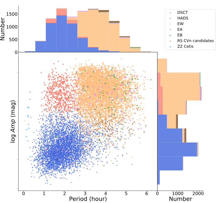
Figure 8: Relation between period and amplitude in logarithmic scale. DSCT, HADS and eclipsing binaries are well separated. A period histogram is at the top, and an amplitude histogram is on the right.

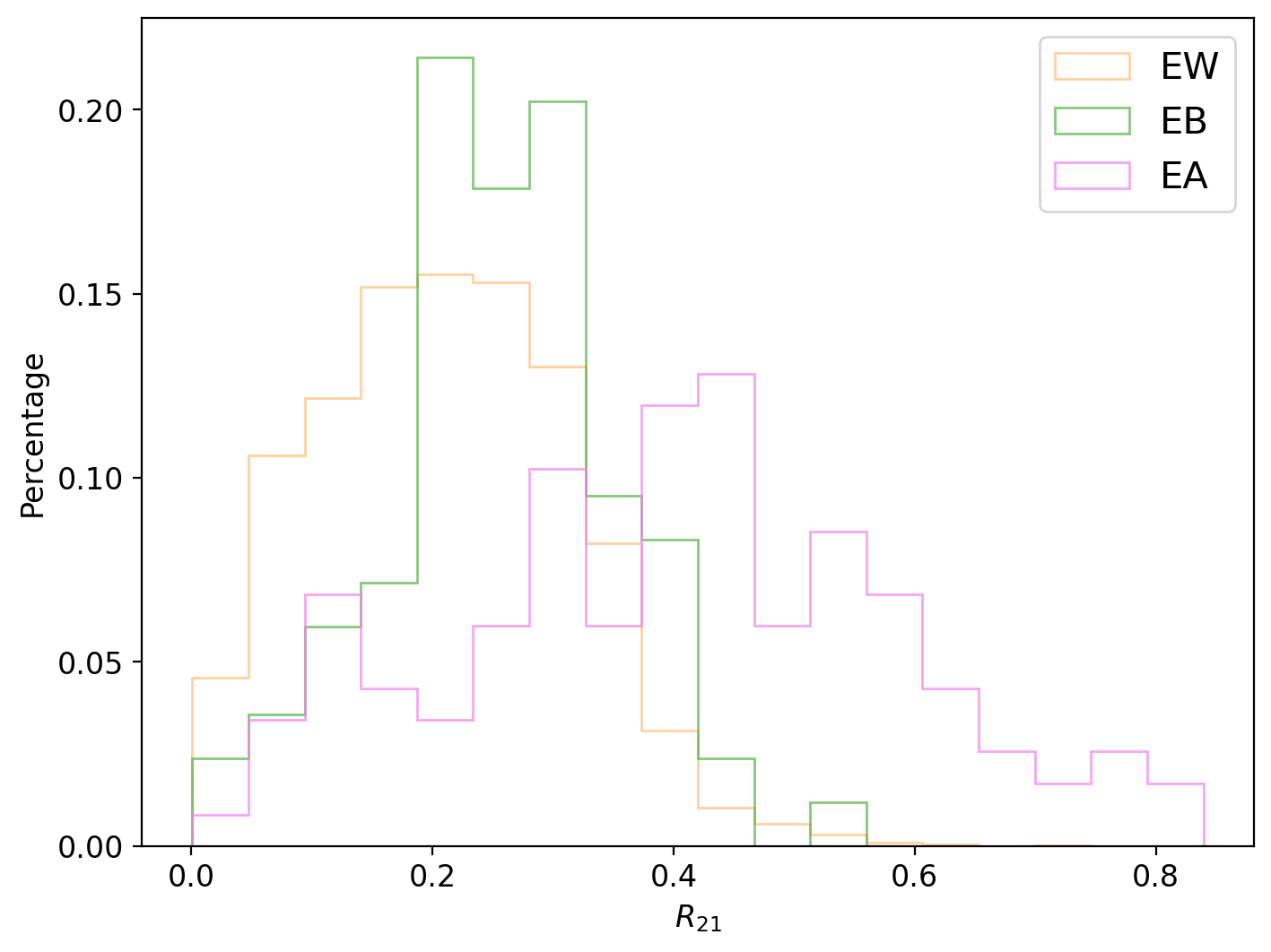
Figure 9: Histogram of $R_{21}$ of EWs, EBs and EAs. Larger $R_{21}$ is correlated with more asymmetric light curve. EAs statistically have largest $R_{21}$, followed by EBs and EWs.

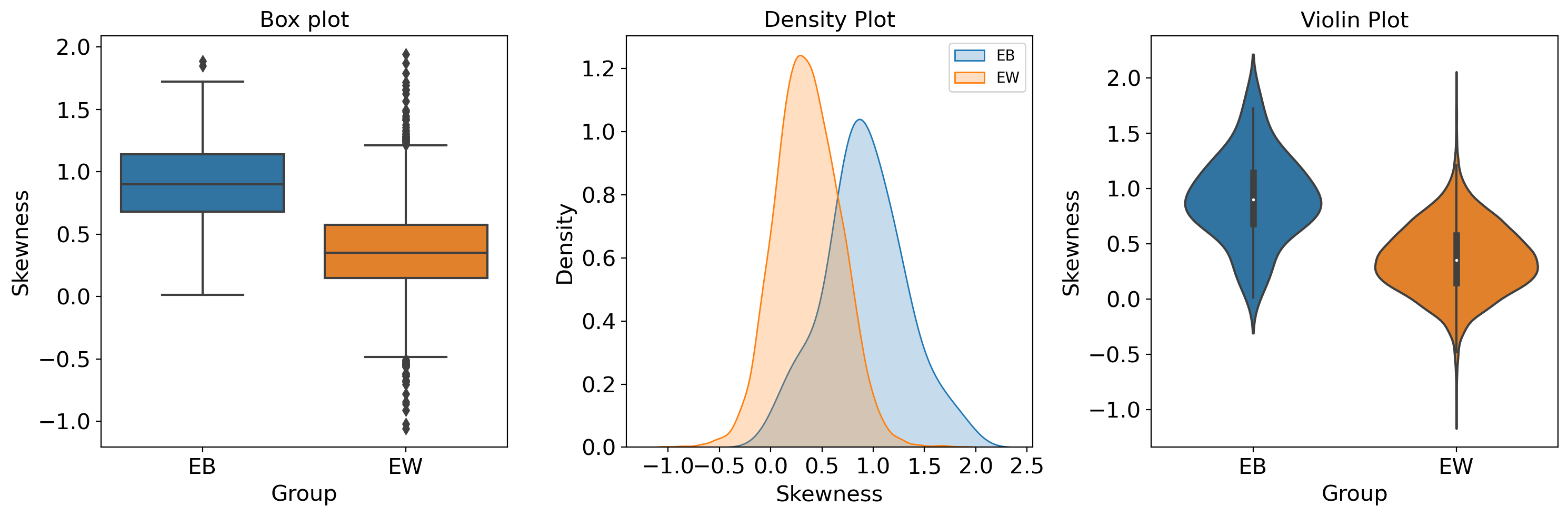
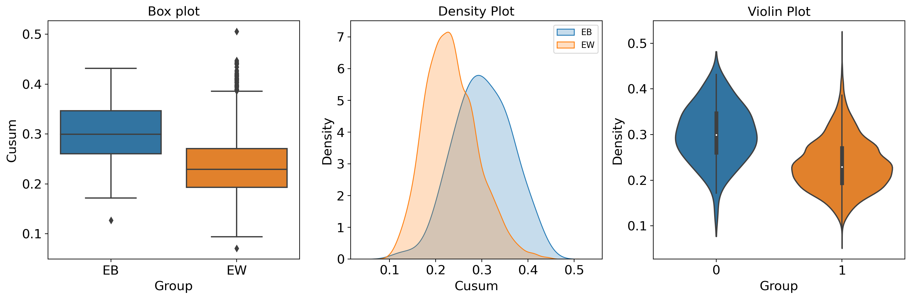
Figure 10: The box plot, density plot and violin plot depicting the distribution of skewness (upper) and cusum (lower) of the light curves of EBs and EWs. Box plot displays the minimum, first quartile, median, third quartile and maximum of a distribution, while density plot represents the probability density function of it. Violin Plot combines the information provided by the box plot and the density plot, using a kernel density estimation on each side.

Table 10: P-values of the K-S test and T-test on skewness, cusum and $R_{21}$ of EBs and EWs.

	K-S test	T-test
Skewness	2.068$\times 10^{-32}$	2.235$\times 10^{-54}$
Cusum	8.094$\times 10^{-17}$	3.954$\times 10^{-27}$
$R_{21}$	7.827$\times 10^{-5}$	4.050$\times 10^{-5}$

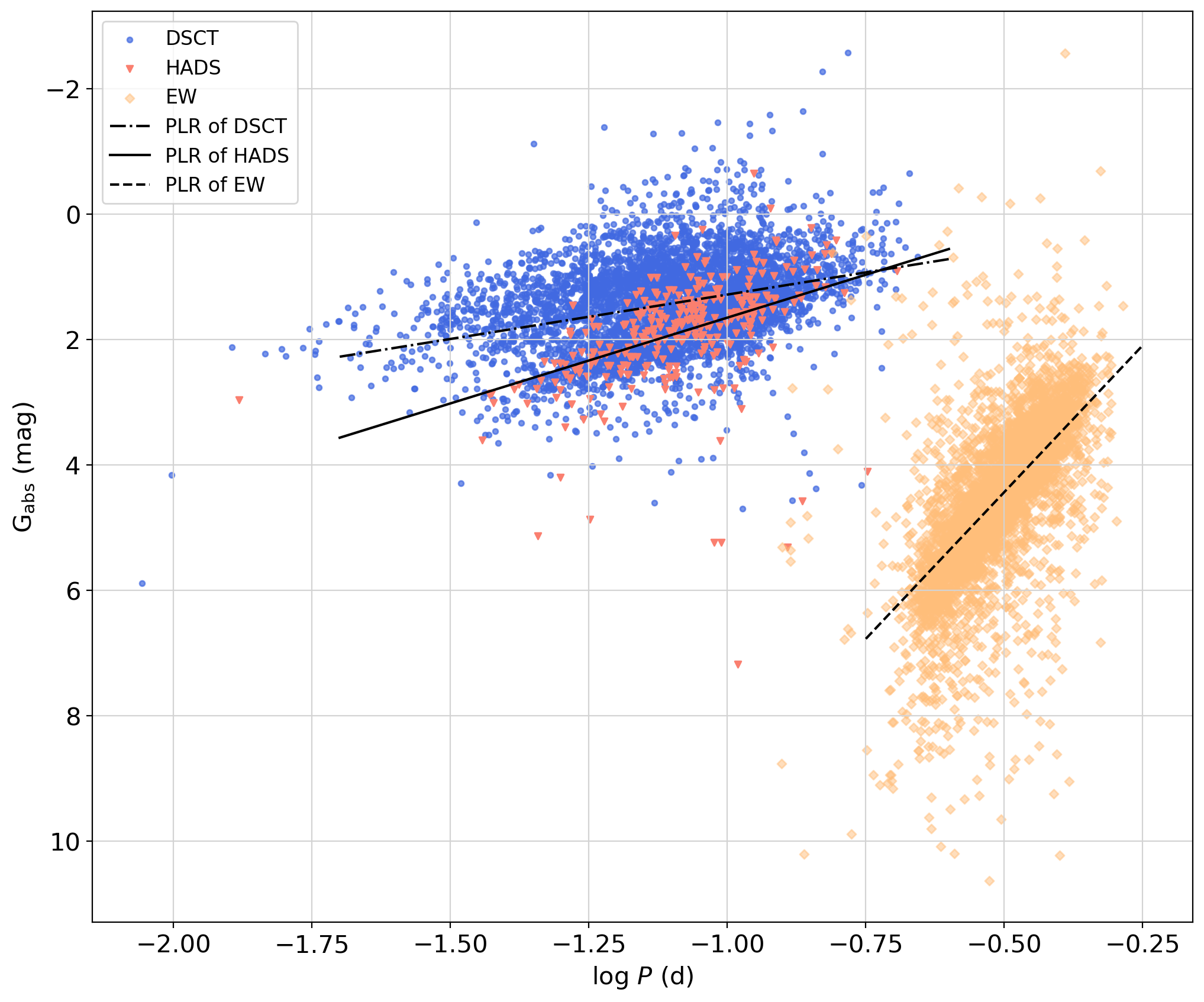
Figure 11: Period-Luminosity Relation of DSCT (dash-dotted line), HADS (solid line) and EW-type eclipsing binaries (dashed line). DSCT and HADS follow distinct $P-L$ relations, possibly due to different pulsation modes.

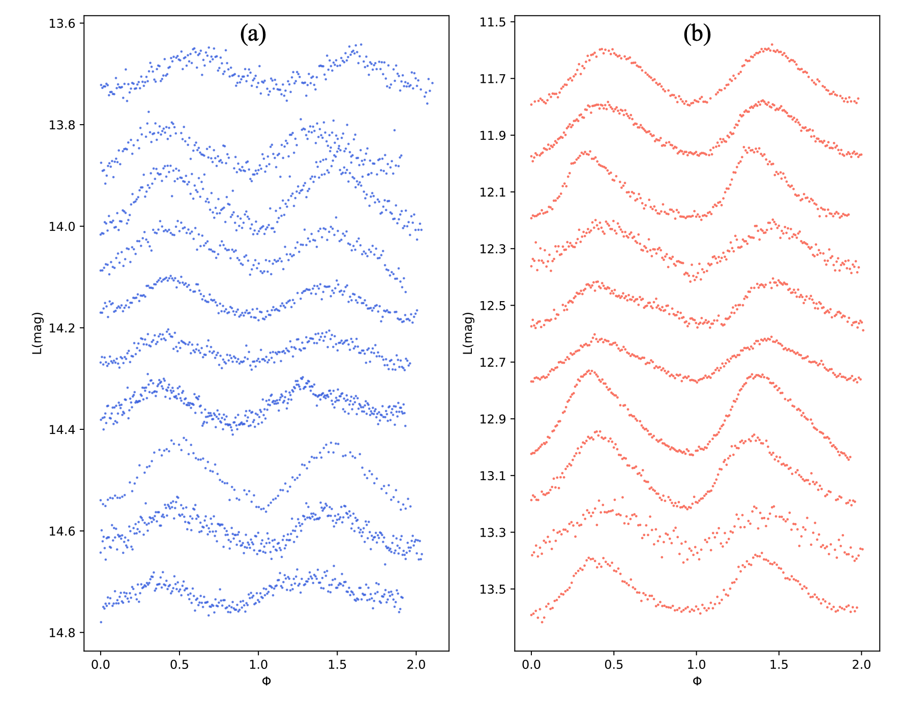
Figure 12: Example light curves of DSCT (a) and HADS (b). The mean magnitudes are fixed at 13.7+0.2i and 11.7+0.2i ($i$ = 0, 1, …, 9) for DSCT and HADS, respectively.

We elaborate on the features used in the machine learning algorithms and the underlying physics, as well as discuss each type of variable stars in detail in this section, including their LC features and Period-Luminosity relations.

5.1 Comprehensive discussion of variable stars

Figure 8 presents the relationship between period and amplitude of the variable stars while quantifying their distribution within each bin. This distribution allows for a rough differentiation between DSCT, HADS, eclipsing binaries and RS CVn candidates. DSCT and HADS typically have shorter periods, with HADS inherently possessing greater amplitudes. Conversely, eclipsing binaries and RS CVn candidates tend to have longer periods, while LCs of the former generally have larger light-variation amplitudes. As shown in Figure 4, period is the most important feature in the classification process. The number of $\delta$ Scuti stars decrease with pulsating period (Rodríguez & Breger, 2001; Qian et al., 2018), and most $\delta$ Scuti stars exhibit periods predominantly below 0.1 d. On the contrary, contact binaries have a short-period cutoff of 0.22 d (some studies have revised this cutoff to 0.15 d, Rucinski 1992; Qian et al. 2020), probably due to the fully convective limit (Rucinski, 1992), timescale of the angular momentum loss (Stepien, 2011), the low mass limit of the primary component (Jiang et al., 2012), etc. Although the cutoff-period refers to the orbital period (twice of the photometric period), most of the binary stars have photometric periods longer than the cutoff period. These trends suggest the presence of a natural period dichotomy between $\delta$ Scuti stars and binaries. It is noteworthy that the majority of $\delta$ Scuti stars in our catalog exhibit periods below 4 h, indicating the efficiency of TMTS in identifying short-period variables.

In Figure 9, the Fourier parameter $R_{21}$ helps to separate EAs, EBs and EWs, especially EAs. $R_{21}$ measures the extent of deviation of a LC from a sinusoidal function, with higher values indicating more substantial deviations. Consequently, EAs exhibit the highest $R_{21}$ values, followed by EBs, while EWs tend to have the lowest values. Moreover, skewness and cusum are paramount contributors in distinguishing EBs from EWs. Skewness quantifies the degree of asymmetry within a distribution, while cusum measures its volatility. Elevated asymmetry and volatility correspond to increased values in both skewness and cusum, as observed in the light curves of EBs. The box plot, density plot and violin plot, depicting the distribution of skewness and cusum of the EBs and EWs in our catalog, are shown in Figure 10. Furthermore, we conducted Kolmogorov-Smirnov (K-S) and T-tests on skewness, cusum and $R_{21}$ of EBs and EWs, with the correspinding p-values listed in Table 10. All p-values, including that of $R_{21}$, are noticeably below 0.0001, indicating a statistically significant distinction in the distribution of skewness, cusum and R21 between EBs and EWs at a significance level of 99.99%.

The nature of eclipse is that the two stars periodically shade each other when orbiting around a common center of mass. As the process is symmetric, the LCs of eclipsing binaries tend to display a higher degree of symmetry. In contrast, driven by the $\kappa$ mechanism, the light curves of $\delta$ Scuti stars typically manifest rapid ascending phases followed by slower descents (saw-tooth-shaped), thereby introducing a higher level of asymmetry. As $\delta$ Scuti stars undergo contraction and expansion periodically, their opacity and luminosities change accordingly. Given that the contraction phase (corresponding to the decrease in the LC) is of a longer duration, the LCs of $\delta$ Scuti stars show a saw-tooth shape (Eddington 1917; Zhevakin 1963).

Given that various types of variable stars tend to occupy distinct regions within the $Gaia$ CMD, it becomes a powerful tool for classification. For instance, $\delta$ Scuti stars are typically found in the instability strip on or above the main sequence in the CMD. Although eclipsing binaries can appear anywhere, the observations conducted by TMTS (with upper-period-bound of 7.5 h) are primarily geared towards detecting $G$-, $K$-, or $M$-type stars (the CMD’s lower right quadrant corresponds to stars with smaller radii, so that the distance between the two stars could be closer, which leads to shorter periods). This limitation naturally segregates eclipsing binaries from $\delta$ Scuti stars, which are typically comprised of $A$- to $F$-type stars.

5.2 $\delta$ Scuti stars

$\delta$ Scuti stars are $A0$- to $F5$-type stars pulsating in radial and non-radial acoustic modes. Their absolute magnitudes are typically below 3.5 mag, with temperature between 6900 K and 8900 K. $\delta$ Scuti stars locate in the intersection of the main sequence and the classical instability strip in the Hertzsprung–Russell diagram (as well as the $Gaia$ CMD). From a stellar evolutionary standpoint, most of them are main sequence stars in the hydrogen-burning stage, and a few may be zero-age main sequence (ZAMS) stars, red giants or blue stragglers moving off the main sequence. The $\kappa$ mechanism accounts for most oscillations seen in $\delta$ Scuti stars, where opacity increases with temperature in H and He ionisation zone. Their pulsation modes are complex, including low and intermediate order pressure modes (p-modes) and gravity modes (g-modes). Some stars are known to have multiple modes, which makes them promising objects for asteroseismological study. Among $\delta$ Scuti stars, HADS typically exhibit radial mode pulsation. With increased photometric precision, non-radial modes have also been detected in some cases. Compared with DSCT, HADS generally have lower rotational velocities (i.e., $v$ sin$i$ $\leq$ 30 km^-1), while $v$ sin$i$ can reach 200 km^-1 for DSCT (McNamara, 1997; Pigulski et al., 2006).

Numerous models have provided theoretical calculations of the instability strip of $\delta$ Scuti stars (Dupret et al., 2004; Xiong et al., 2016). However, the theoretical edges does not match the observed pulsator fraction (Murphy et al., 2019). The new identification of over 4000 $\delta$ Scuti stars in our catalogue not only helps to better constrain the edges of the instability strip, but also offers valuable insights into the pulsator fraction inside the strip.

$P-L$ relations have been established for various pulsating stars (Leavitt & Pickering, 1912). Among them, the $P-L$ relations of Cepheids have been extensively studied. Like other pulsating stars, $\delta$ Scuti stars also follow $P-L$ relations (Breger & Bregman, 1975; McNamara, 1997), which offers an independent avenue for calibrating cosmic distances, complementary to the Cepheids. However, due to their intricate pulsation modes, lower luminosity and smaller amplitudes, the $P-L$ relations of $\delta$ Scuti stars has remained comparatively less well-defined (Ziaali et al., 2019). Figure 11 shows the P-L relations of DSCT, HADS and EW-type eclipsing binaries in our catalogues. We will discuss the $P-L$ relation of EWs later. The best fitting $P-L$ relations of DSCT and HADS in our catalog are as follow:

$$\mathrm{DSCT}:G\mathrm{{}_{abs}}=-1.42\log(\frac{P}{\rm 1~{}d})-0.13\ \ ({\rm mag})$$ (5)

$$\mathrm{HADS}:G\mathrm{{}_{abs}}=-2.74\log(\frac{P}{\rm 1~{}d})-1.08\ \ ({\rm mag})$$ (6)

The increased dispersion observed in the $P-L$ relation of DSCT, as compared to HADS, can be ascribed to the fact that DSCT undergo multi-mode pulsations, encompassing both overtone mode and fundamental mode, whereas HADS predominantly exhibit fundamental mode pulsations. As expected, the overtone mode pulsation corresponds to a brighter $P-L$ relation compared to the fundamental mode (see also Lin et al. 2023c). Additionally, the overtone mode comprises a blend of various overtone modes, which may explain the larger dispersion and is consistent with Jayasinghe et al. (2020). In the short-period end of the period-luminosity diagram, the distribution of DSCT appears relatively sparse, forming what seems like two distinct lines, one aligns with the dash-dotted line ($P-L$ relation of DSCT), while the other corresponds to the solid line ($P-L$ relation of HADS). This may be attributed to the possibility that within the DSCT class, stars pulsating in the fundamental mode and overtone mode adhere to different $P-L$ relations. Conducting separate fittings of the $P-L$ relations for DSCT with distinct pulsation modes contributes to enhancing the accuracy of the $P-L$ relation. Further discussion and comparison of the $P-L$ relations will be undertaken in our future work (Chen L, et al., in prep.).

Figure 12 shows some light curves of DSCT (a) and HADS (b). HADS commonly exhibit LCs characterized by a rapid rise and slow decline, while DSCT show a broader range of LC shapes, including more sinusoidal patterns.

5.3 Eclipsing Binaries

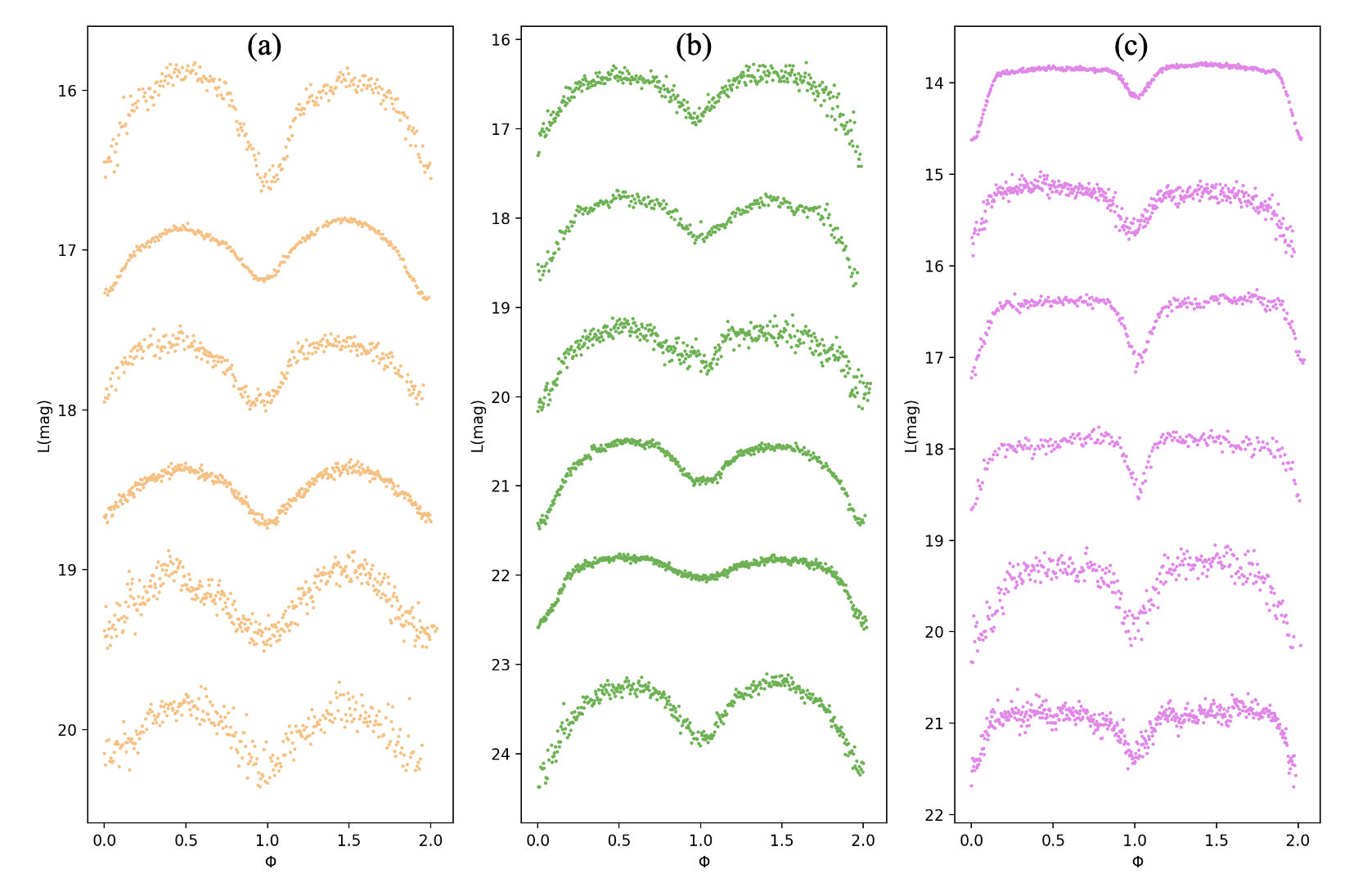
Figure 13: Example light curves of EW-type eclipsing binaries (a), EB-type eclipsing binaries (b) and EA-type eclipsing binaries (c). The mean magnitudes are fixed at 16.2+0.8i, 16.6+1.1i, and 14.2+1.5i ($i$ = 0, 1, …, 5) for EWs, EBs and EAs, respectively.

Eclipsing binary exhibits eclipses due to the nearly edge-on orientation of its orbital plane with respect to the Earth, causing periodic changes in its brightness as one star passes in front of its companion. Unlike pulsating stars, they can appear anywhere in the CMD (Eyer et al., 2019). Eclipsing binaries offer unique opportunities for investigating material exchange and common envelope evolution due to the intricate interactions between the two components (Stassun et al., 2014; Pols et al., 1997; Nelson et al., 2023).

Eclipsing binaries can be categorized into three types based on their LC shapes, among which EWs accounts for the highest proportion, as illustrated in Figure 2 and Table 4. Figure 13 displays typical light curves of the EWs (a), EB(b) and EAs (c). EAs exhibit clearly defined moments of beginning and end of the eclipse. Typically, there is minimum material exchange between the two spherical or slightly ellipsoidal stars, and they may be detached or semi-detached. In contrast, stars in the EB-type systems have active mass transfer between the envelopes, leading to continuous LC variations that make it impossible to determine the exact start and end moments of the eclipse. Additionally, EBs are characterized by different primary and secondary minimum depths, which distinguishes them from EW-type binaries. Finally, EWs are marked by nearly equal depths in their primary and secondary minima. Both components fill their Roche Lobes in EW-type systems. In addition, the densely sampled TMTS LCs would greatly contribute to the determination of minima epoch of eclipsing binaries in our catalogues.

EW-type eclipsing binaries also follow a $P-L$ relation, especially in infrared bands, owing to the strong geometric constraints imposed by the common envelope (Rucinski, 2004; Ren et al., 2021). In simple terms, orbital periods are correlated with radius of the system, and therefore with its luminosity. This $P-L$ relation renders EWs as reliable distance indicators. Compared to Cepheids and RR Lyrae stars, EWs trace older stellar population than Cepheids and are more common in open clusters and the solar neighborhood than RR Lyrae stars. This highlights their unique value as distance tracers (Chen et al., 2016). However, owing to the limited sample size, the determination of $P-L$ relations for EWs is characterized by less precision, which impedes their application. Chen et al. (2018) studied 27,318 EWs with accurate distance measurements, and they reached an distance accuracy of 8%. Figure 11 shows the $P-L$ relation of EWs in our catalogue, the best fitting is

$$G\mathrm{{}_{abs}}=-9.36\log(\frac{P}{\rm 1~{}d})-0.25\ \ ({\rm mag})$$ (7)

Orbital period is used in this fitting. The $P-L$ relation of EWs may be influenced by factors such as color and metallicity (Rucinski, 2004), and we only provide the simplest analysis in this paper.

5.4 RS CVn

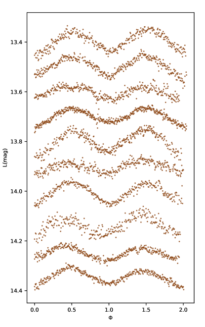
Figure 14: Example light curves of RS CVn candidates. The mean magnitudes are fixed at 13.4+0.1i ($i$ = 0, 1, …, 9).

RS CVn variables are an active subclass of binary systems characterized by strong Ca II H & K emission lines emerged from at least one of the system’s components (Hall, 1976). Consequently, the periodic photometric variations in these systems arise not only from pulsations or eclipses, but also from their rotation. The primary star of RS CVn is a F to K-type subgiant or giant star, with a G to M-type dwarf or subgiant companion (Martínez et al., 2022; Fekel et al., 1986). The orbital periods of RS CVn variables exhibit variability over time, and studying these changes would shed light on the mass loss process, magnetic field interactions and the dynamic evolution of binary systems (Hall & Kreiner, 1980). It’s crucial to mention that a comprehensive understanding of RS CVn variables requires detailed spectral properties. Therefore, in this paper, we only present a catalogue of RS CVn candidates.

The LCs of RS CVn variables exhibit a discernible semiperiodic pattern, which coexists alongside the eclipse features. This phenomenon is attributed to the presence of “starspots”. Arising from strong magnetic fields and stifled convection, these starspots are cooler regions on the photosphere in the outer layer of the star (Roettenbacher et al., 2015). Figure 14 shows the LCs of some RS CVn candidates in our catalogue.

6 Summary

With a cadence of ~1 minute, TMTS has shown great potential in the detection of short-period variables. In this paper, we systematically classified 11,638 variable stars into 6 main categories using the state-of-the-art XGBoost and Random Forest algorithms, achieving remarkable accuracy levels of 98.83% and 98.73%, respectively. We constructed a well-chosen training and test dataset of 4506 light curves of the variables. Period is the most important feature in the classification, followed by features that characterize the shape of the LCs as well as $Gaia$ $G$_abs and $(B\mathrm{{}_{p}}-R\mathrm{{}_{p}})_{0}$, which is in accordance with our predictions. Once the effectiveness of the classifiers was confirmed, we utilized them to assign labels to the remaining unlabeled light curves. Notably, in both classifiers, the macro-average and weighted-average F₁ scores are higher than 98%, with the F₁ scores for DSCT, EA, EB and HADS exceeds 99%, demonstrating the effectiveness of our feature selection and model training methodologies. To ensure the quality of the catalogue, we conducted a manual inspection to all included light curves. The period-amplitude diagram and the period-$R_{21}$ diagram prove the validity of the classification.

We identified 5504 $\delta$ Scuti stars (including 4876 typical $\delta$ Scuti stars and 628 high-amplitude $\delta$ Scuti stars), 5899 eclipsing binaries (including 117 EAs, 84 EBs and 5698 EWs) and 226 candidates of RS Canum Venaticorum systems. Additionally, with the help of color-magnitude diagram established from the Gaia database, we discovered 9 ZZ Ceti stars. Combining Galactic longitudes with metal abundances, we discovered 8 metal-poor $\delta$ Scuti stars (SX Phe stars). Among the 4876 DSCT in our catalog, 4297 were newly discovered, and most of them have periods shorter than 4 hours, showing the ability of TMTS to search for short-period variables. The newly-identified $\delta$ Scuti stars could help to better refine the red and blue edges of the instability strip. We study the period-luminosity relations of DSCT, HADS and EW-type eclipsing binaries. The subclasses of DSCT and HADS follow distinct $P-L$ relations, and different $P-L$ relations seem to also exist within the class of DSCT, potentially attributable to the difference in fundamental mode and overtone mode pulsations. An in-depth analysis of $\delta$ Scuti stars with varying pulsation modes would contribute to a more precise determination of the $P-L$ relation. We will further discuss DSCT, HADS and their $P-L$ relations in the forthcoming paper.

Data Availability

The catalogues are all available from this paper and CDS.

References

- Abbott et al. (2017) Abbott B. P., et al., 2017, Physical review letters, 119, 161101
- Abbott et al. (2020) Abbott R., et al., 2020, The Astrophysical Journal Letters, 896, L44
- Bishop (1994) Bishop C. M., 1994, Review of scientific instruments, 65, 1803
- Bloom et al. (2012) Bloom J., et al., 2012, Publications of the Astronomical Society of the Pacific, 124, 1175
- Breger (2000) Breger M., 2000, in Delta Scuti and Related Stars. p. 3
- Breger & Bregman (1975) Breger M., Bregman J. N., 1975, Astrophysical Journal, Vol. 200, p. 343-353, 200, 343
- Breiman (2001) Breiman L., 2001, Machine learning, 45, 5
- Brown et al. (2011) Brown W. R., Kilic M., Hermes J., Prieto C. A., Kenyon S. J., Winget D., 2011, The Astrophysical Journal Letters, 737, L23
- Brown et al. (2018) Brown A., et al., 2018, Astronomy & astrophysics, 616, A1
- Burdge et al. (2019) Burdge K. B., et al., 2019, Nature, 571, 528
- Caiazzo et al. (2021) Caiazzo I., et al., 2021, Nature, 595, 39
- Chang et al. (2013) Chang S.-W., Protopapas P., Kim D.-W., Byun Y.-I., 2013, The Astronomical Journal, 145, 132
- Chawla et al. (2002) Chawla N. V., Bowyer K. W., Hall L. O., Kegelmeyer W. P., 2002, Journal of artificial intelligence research, 16, 321
- Chen et al. (2015) Chen T., et al., 2015, R package version 0.4-2, 1, 1
- Chen et al. (2016) Chen X., De Grijs R., Deng L., 2016, The Astrophysical Journal, 832, 138
- Chen et al. (2018) Chen X., Deng L., De Grijs R., Wang S., Feng Y., 2018, The Astrophysical Journal, 859, 140
- Chen et al. (2020a) Chen X., Wang S., Deng L., De Grijs R., Yang M., Tian H., 2020a, The Astrophysical Journal Supplement Series, 249, 18
- Chen et al. (2020b) Chen W.-C., Liu D.-D., Wang B., 2020b, The Astrophysical Journal Letters, 900, L8
- Cohen & Sarajedini (2012) Cohen R. E., Sarajedini A., 2012, Monthly Notices of the Royal Astronomical Society, 419, 342
- Copperwheat et al. (2011) Copperwheat C., et al., 2011, Monthly Notices of the Royal Astronomical Society, 410, 1113
- Dong et al. (2020) Dong X., Yu Z., Cao W., Shi Y., Ma Q., 2020, Frontiers of Computer Science, 14, 241
- Drake et al. (2014) Drake A., et al., 2014, The Astrophysical Journal Supplement Series, 213, 9
- Dupret et al. (2004) Dupret M.-A., Grigahcene A., Garrido R., Gabriel M., Scuflaire R., 2004, Astronomy & Astrophysics, 414, L17
- Eddington (1917) Eddington A., 1917, The Observatory, Vol. 40, p. 290-293 (1917), 40, 290
- Eyer et al. (2019) Eyer L., et al., 2019, Astronomy & Astrophysics, 623, A110
- Fekel et al. (1986) Fekel F. C., Moffett T. J., Henry G. W., 1986, Astrophysical Journal Supplement Series (ISSN 0067-0049), vol. 60, Feb. 1986, p. 551-576. NASA-supported research., 60, 551
- Fontaine et al. (2003) Fontaine G., Bergeron P., Billeres M., Charpinet S., 2003, The Astrophysical Journal, 591, 1184
- Gorski et al. (2005) Gorski K. M., Hivon E., Banday A. J., Wandelt B. D., Hansen F. K., Reinecke M., Bartelmann M., 2005, The Astrophysical Journal, 622, 759
- Guo et al. (2023) Guo J., et al., 2023, Monthly Notices of the Royal Astronomical Society, 523, 1591
- Guo et al. (2024) Guo J., et al., 2024, Monthly Notices of the Royal Astronomical Society, p. stae290
- Hall (1976) Hall D. S., 1976, in International Astronomical Union Colloquium. pp 287–348
- Hall & Kreiner (1980) Hall D., Kreiner J., 1980, Acta Astronomica, 30, 387
- Handler (2009) Handler G., 2009, in AIP Conference Proceedings. pp 403–409
- Heinze et al. (2018) Heinze A., et al., 2018, The Astronomical Journal, 156, 241
- Holdsworth et al. (2014) Holdsworth D. L., et al., 2014, Monthly Notices of the Royal Astronomical Society, 439, 2078
- Holl et al. (2018) Holl B., et al., 2018, Astronomy & Astrophysics, 618, A30
- Hosenie et al. (2020) Hosenie Z., Lyon R., Stappers B., Mootoovaloo A., McBride V., 2020, Monthly Notices of the Royal Astronomical Society, 493, 6050
- Ivezić et al. (2019) Ivezić Ž., et al., 2019, The Astrophysical Journal, 873, 111
- Iwanek et al. (2022) Iwanek P., et al., 2022, The Astrophysical Journal Supplement Series, 260, 46
- Jayasinghe et al. (2019) Jayasinghe T., et al., 2019, Monthly Notices of the Royal Astronomical Society, 486, 1907
- Jayasinghe et al. (2020) Jayasinghe T., et al., 2020, Monthly Notices of the Royal Astronomical Society, 493, 4186
- Jiang et al. (2012) Jiang D., Han Z., Ge H., Yang L., Li L., 2012, Monthly Notices of the Royal Astronomical Society, 421, 2769
- Jordi et al. (2010) Jordi C., et al., 2010, Astronomy & Astrophysics, 523, A48
- Kim & Bailer-Jones (2016) Kim D.-W., Bailer-Jones C. A., 2016, Astronomy & Astrophysics, 587, A18
- Kim et al. (2002) Kim C., Jeon Y.-B., Kim S.-L., 2002, Astrophysics and space science, 282, 731
- Kim et al. (2014) Kim D.-W., Protopapas P., Bailer-Jones C. A., Byun Y.-I., Chang S.-W., Marquette J.-B., Shin M.-S., 2014, Astronomy & Astrophysics, 566, A43
- Krakowski et al. (2016) Krakowski T., Małek K., Bilicki M., Pollo A., Kurcz A., Krupa M., 2016, Astronomy & Astrophysics, 596, A39
- Kupfer et al. (2021) Kupfer T., et al., 2021, Monthly Notices of the Royal Astronomical Society, 505, 1254
- Leavitt & Pickering (1912) Leavitt H. S., Pickering E. C., 1912, Harvard College Observatory Circular, vol. 173, pp. 1-3, 173, 1
- Lin et al. (2022) Lin J., et al., 2022, Monthly Notices of the Royal Astronomical Society, 509, 2362
- Lin et al. (2023a) Lin J., et al., 2023a, A seven-Earth-radius helium-burning star inside a 20.5-min detached binary (arXiv:2312.13612)
- Lin et al. (2023b) Lin J., et al., 2023b, Nature Astronomy, 7, 223
- Lin et al. (2023c) Lin J., et al., 2023c, MNRAS, 523, 2172
- Liu et al. (2023) Liu Q., et al., 2023, MNRAS, 523, 2193
- Lomb (1976) Lomb N. R., 1976, Astrophysics and space science, 39, 447
- Long et al. (2012) Long J. P., El Karoui N., Rice J. A., Richards J. W., Bloom J. S., 2012, Publications of the Astronomical Society of the Pacific, 124, 280
- Martínez et al. (2022) Martínez C., Mauas P., Buccino A., 2022, Monthly Notices of the Royal Astronomical Society, 512, 4835
- McNamara (1997) McNamara D., 1997, Publications of the Astronomical Society of the Pacific, 109, 1221
- McNamara (2011) McNamara D., 2011, The Astronomical Journal, 142, 110
- Murphy et al. (2019) Murphy S. J., Hey D., Van Reeth T., Bedding T. R., 2019, Monthly Notices of the Royal Astronomical Society, 485, 2380
- Naul et al. (2018) Naul B., Bloom J. S., Pérez F., van der Walt S., 2018, Nature Astronomy, 2, 151
- Nelson et al. (2023) Nelson R., Terrell D., Milone E., 2023, New Astronomy Reviews, p. 101684
- Nixon & Madhusudhan (2020) Nixon M. C., Madhusudhan N., 2020, Monthly Notices of the Royal Astronomical Society, 496, 269
- Pigulski et al. (2006) Pigulski A., Kolaczkowski Z., Ramza T., Narwid A., 2006, Memorie della Società Astronomica Italiana, v. 77, p. 223 (2006), 77, 223
- Plavec (1968) Plavec M., 1968, in , Vol. 6, Advances in Astronomy and Astrophysics. Elsevier, pp 201–278
- Pols et al. (1997) Pols O. R., Tout C. A., Schröder K.-P., Eggleton P. P., Manners J., 1997, Monthly Notices of the Royal Astronomical Society, 289, 869
- Postnov & Yungelson (2014) Postnov K. A., Yungelson L. R., 2014, Living Reviews in Relativity, 17, 1
- Qian et al. (2018) Qian S., Li L., He J., Zhang J., Zhu L., Han Z., 2018, Monthly Notices of the Royal Astronomical Society, 475, 478
- Qian et al. (2020) Qian S.-B., Zhu L.-Y., Liu L., Zhang X.-D., Shi X.-D., He J.-J., Zhang J., 2020, Research in Astronomy and Astrophysics, 20, 163
- Rebassa-Mansergas et al. (2019) Rebassa-Mansergas A., Toonen S., Korol V., Torres S., 2019, Monthly Notices of the Royal Astronomical Society, 482, 3656
- Ren et al. (2021) Ren F., Chen X., Zhang H., de Grijs R., Deng L., Huang Y., 2021, The Astrophysical Journal Letters, 911, L20
- Richards et al. (2011) Richards J. W., et al., 2011, The Astrophysical Journal, 733, 10
- Riess et al. (2018) Riess A. G., et al., 2018, The Astrophysical Journal, 861, 126
- Rodríguez (2004) Rodríguez E., 2004, Monthly Notices of the Royal Astronomical Society, 352, L11
- Rodríguez & Breger (2001) Rodríguez E., Breger M., 2001, Astronomy & Astrophysics, 366, 178
- Roettenbacher et al. (2015) Roettenbacher R. M., et al., 2015, The Astrophysical Journal, 807, 23
- Rucinski (1992) Rucinski S., 1992, The Astronomical Journal, 103, 960
- Rucinski (2004) Rucinski S. M., 2004, New Astronomy Reviews, 48, 703
- Sandage et al. (2006) Sandage A., Tammann G., Saha A., Reindl B., Macchetto F., Panagia N., 2006, The Astrophysical Journal, 653, 843
- Scargle (1982) Scargle J. D., 1982, Astrophysical Journal, Part 1, vol. 263, Dec. 15, 1982, p. 835-853., 263, 835
- Soszynski et al. (2014) Soszynski I., et al., 2014, arXiv preprint arXiv:1410.1542
- Soszyński et al. (2021) Soszyński I., et al., 2021, arXiv preprint arXiv:2111.03072
- Stassun et al. (2014) Stassun K. G., Feiden G. A., Torres G., 2014, New Astronomy Reviews, 60, 1
- Stepien (2011) Stepien K., 2011, arXiv preprint arXiv:1105.2645
- Taam & Sandquist (2000) Taam R. E., Sandquist E. L., 2000, Annual Review of Astronomy and Astrophysics, 38, 113
- Theuns & Jorissen (1993) Theuns T., Jorissen A., 1993, Monthly Notices of the Royal Astronomical Society, 265, 946
- Udalski et al. (2015) Udalski A., Szymański M., Szymański G., 2015, arXiv preprint arXiv:1504.05966
- Watson et al. (2006) Watson C. L., Henden A. A., Price A., 2006, in Society for Astronomical Sciences Annual Symposium. p. 47
- Xiong et al. (2016) Xiong D., Deng L., Zhang C., Wang K., 2016, Monthly Notices of the Royal Astronomical Society, 457, 3163
- Zhang & Bloom (2021) Zhang K., Bloom J. S., 2021, Monthly Notices of the Royal Astronomical Society, 505, 515
- Zhang et al. (2020) Zhang J.-C., et al., 2020, Publications of the Astronomical Society of the Pacific, 132, 125001
- Zhevakin (1963) Zhevakin S., 1963, Annual Review of Astronomy and Astrophysics, 1, 367
- Ziaali et al. (2019) Ziaali E., Bedding T. R., Murphy S. J., Van Reeth T., Hey D. R., 2019, Monthly Notices of the Royal Astronomical Society, 486, 4348