Abstract

This paper introduces Dual Interior Point Learning (DIPL) and Dual Supergradient Learning (DSL) to learn dual feasible solutions to parametric linear programs with bounded variables, which are pervasive across many industries. DIPL mimics a novel dual interior point algorithm while DSL mimics classical dual supergradient ascent. DIPL and DSL ensure dual feasibility by predicting dual variables associated with the constraints then exploiting the flexibility of the duals of the bound constraints. DIPL and DSL complement existing primal learning methods by providing a certificate of quality. They are shown to produce high-fidelity dual-feasible solutions to large-scale optimal power flow problems providing valid dual bounds under $0.5\%$ optimality gap.

1 Introduction

Consider parametric optimization problems of the form

$$(\text{P}_{\beta})\quad\min_{\mathbf{x}}\quad \mathbf{c}_{\beta}^{\top}\mathbf{x}$$

s.t. $$\mathbf{A}_{\beta}\mathbf{x}=\mathbf{b}_{\beta}$$

$$\mathbf{l}_{\beta}\leq\mathbf{x}\leq\mathbf{u}_{\beta}$$

where $\beta$ represents instance parameters that determine the objective costs $\mathbf{c}_{\beta}$, the constraint coefficients $\mathbf{A}_{\beta}$, the constraint constants $\mathbf{b}_{\beta}$, and the variable bounds $\mathbf{l}_{\beta}$ and $\mathbf{u}_{\beta}$. Such problems are ubiquitous in industry; for instance, independent system operators run economic dispatch optimizations every five minutes in the United States and semi-conductor manufacturers run such large optimizations for planning their fabrication plants on a daily basis. Since many such problems operate on physical infrastructures that change relatively slowly, it is reasonable to assume that the instance parameters $\beta$ are characterized by a distribution learned from historical data. The bound constraints are also natural in practice, since most industrial optimization problems operate on infrastructures with finite resources.

The goal of this paper is to learn a Dual Optimization Proxy, i.e., a model that returns a dual-feasible solution to an instance $\text{P}_{\beta}$. Primal optimization proxies, which produce feasible solutions to parametric optimization problems, have received significant attention in recent years (e.g., Chen et al. (2023)). Dual optimization proxies complement primal optimization proxies by providing certificates of quality.

To learn a dual optimization proxy for $\text{P}_{\beta}$, the paper proposes the novel concept of Dual Interior-Point Learning (DIPL), a self-supervised learning method that combines the “Predict then Complete” (PTC) paradigm and the interior point method to linear programming. The high-level idea underlying PTC is to predict the dual variables ${\bf y}$ associated with the constraints $\mathbf{A}_{\beta}\mathbf{x}=\mathbf{b}_{\beta}$ and to use the flexibility of the dual variables $\mathbf{z}^{l}$ and $\mathbf{z}^{u}$ associated with the bounds to complete the solution and ensure dual feasibility. DIPL learns $\text{P}_{\beta}$ by mimicking a novel dual interior point optimization algorithm that solves for $\mathbf{y}$ and recovers $\mathbf{z}^{l}$ and $\mathbf{z}^{u}$. The paper contributions can be summarized as follows:

• The paper presents a dual solution completion scheme which naturally yields the classical dual supergradient ascent algorithm.

• The paper proposes the Dual Interior Gradient Algorithm for solving the dual barrier problem.

• The paper proposes Dual Supergradient Learning (DSL) and Dual Interior-Point Learning (DIPL) to learn dual-feasible solutions of linear programming problems with bounded variables. DSL and DIPL mimic, in the machine learning context, the dual supergradient ascent and the dual interior gradient algorithms.

• The paper evaluates DSL and DIPL on large-scale optimal power flow problems and shows that they produce high-fidelity dual-feasible solutions providing valid dual bounds. Both achieve under $0.5\%$ mean optimality gap on the largest test case with DIPL consistently outperforming DSL.

The rest of the paper is organized as follows. Section 2 discusses the related work and Section 3 provides the mathematical background. Section 4 introduces the two dual ascent optimization algorithms at the core of DSL and DIPL. Section 5 presents DSL and DIPL, the self-supervised dual optimization learning methods. Section 6 contains the experimental results and Section 7 concludes the paper.

2 Related Work

2.1 Learning for Parametric Optimization

Most research on learning for parametric optimization problems has focused on approximating primal solutions. See, for instance, Park & Van Hentenryck (2023) and the reference therein for a review of some existing methods. In that context, a significant challenge is to ensure that a predicted primal solution satisfies the problem’s constraints.

To that end, most recent works aiming at learning to solve parametric optimization problems are based on mimicking a constrained optimization algorithm. For instance, physics-informed approaches such as Fioretto et al. (2020); Donti et al. (2021) employ a penalty method, wherein the training loss is augmented by a term penalizing constraint violations. The Primal-Dual Learning (PDL) scheme Park & Van Hentenryck (2023) mimics the augmented Lagrangian algorithm. PDL requires both a primal and a dual network, but does not provide any guarantee of feasibility or optimality. In Qian et al. (2023), the authors use a Graph Neural Network (GNN) to emulate the steps taken by an interior-point method. The approach of Qian et al. (2023) is a supervised learning scheme, requiring a dataset of problems to be solved prior to training using an interior-point method with each iterate stored. Despite an existence result for a GNN model that perfectly emulates the steps of IPM, no guarantees on feasibility nor optimality are provided in practice. More recently, Chen et al. (2023) introduced an end-to-end feasible architecture for DC optimal power flow problems, thus providing primal feasibility guarantees. However, the approach of Chen et al. (2023) is problem-specific, and cannot handle general problems.

In contrast, learning dual solutions has received little attention. To the authors’ knowledge, the Dual Conic Proxy (DCP) method for Optimal Power Flow Qiu et al. (2023) is the only such work with formal guarantees. In fact, DCP can be seen as a particular case of DSL, applied to a specific second-order-cone (SOC) formulation. The dual completion procedure of DCP uses problem-specific dual reductions to ensure dual feasibility and eliminate the need to predict some dual variables. In contrast, the proposed DSL and DIPL approaches require minimal assumptions, and are applicable to a broad class of problems.

2.2 First-order Interior-Point Methods

To the authors’ knowledge, the dual interior-point gradient ascent algorithm at the core of DIPL is novel. While dual subgradient methods, like the one that underlies DSL, have been extensively studied Boyd & Mutapcic (2006); Shor et al. (2012), general-purpose linear optimization software mostly rely on simplex and interior-point algorithms. Nevertheless, recent work in large-scale linear optimization Applegate et al. (2021) has demonstrated the benefits of first-order methods.

The idea of smoothing the dual problem by considering its barrier formulation and applying a first-order method is well-known; see Nesterov (2005) for a general treatment of how to minimize non-smooth functions. The authors are not aware of any optimization software that implements the proposed dual interior-point gradient algorithm (see Section 4.2). In addition, to the authors’ knowledge, this paper is the first to embed it in a machine learning context.

The most-closely related algorithm is the ABIP method proposed in Tianyi Lin & Zhang (2021), which uses ADMM to solve for a central solution at each step of its interior-point method. The proposed algorithm differs from ABIP in its use of gradient ascent to solve the dual problem rather than ADMM. In particular, unlike ADMM, the proposed algorithm does not require solving any linear system.

3 Background

Notations

Bold lowercase letters refer to vectors and bold uppercase letters refer to matrices. Scalars are denoted by non-bold letters. The $\odot$ symbol represents element-wise multiplication. A vector in the denominator of a fraction represents element-wise division. Similarly, exponents on vectors represent element-wise exponentiation.

The positive and negative parts of $x\,{\in}\,\mathbb{R}$ are denoted by $|x|^{+}\,{=}\,\max(0,x)$ and $|x|^{-}\,{=}\,\max(0,-x)$. Note that $|x|^{+},|x|^{-}\,{\geq}\,0$ and that $x=|x|^{+}\,{-}\,|x|^{-}$. For vector $\mathbf{x}\,{\in}\,\mathbb{R}^{n}$, the notations $|\mathbf{x}|^{+},|\mathbf{x}|^{-}$ denote the element-wise positive and negative parts, respectively.

Bounded Standard Form

This paper considers parametric linear programs of the form

$$(\text{P}_{\beta})\quad\min_{\mathbf{x}}\quad \mathbf{c}_{\beta}^{\top}\mathbf{x}$$ (2a)

s.t. $$\mathbf{A}_{\beta}\mathbf{x}=\mathbf{b}_{\beta}$$ (2b)

$$\mathbf{l}_{\beta}\leq\mathbf{x}\leq\mathbf{u}_{\beta}$$ (2c)

where $(\mathbf{c}_{\beta},\,\mathbf{l}_{\beta},\,\mathbf{u}_{\beta},\,\mathbf{x})\in\mathbb{R}^{n}$, $\mathbf{b}_{\beta}\in\mathbb{R}^{m}$, and $\mathbf{A}_{\beta}\in\mathbb{R}^{m\times n}$. The subscript $\beta$ is dropped in what follows for brevity. It is assumed that the variable bounds are non-trivial and consistent, i.e., $\mathbf{l}_{\beta}<\mathbf{u}_{\beta}$, and that the primal problem is feasible.

The dual of the problem is given by

$$(\text{D}_{\beta})\quad\max_{\mathbf{y}}\quad \mathbf{b}^{\top}\mathbf{y}+\mathbf{l}^{\top}\mathbf{z}^{l}-\mathbf{u}^{\top}\mathbf{z}^{u}$$ (3a)

s.t. $$\mathbf{A}^{\top}\mathbf{y}+\mathbf{z}^{l}-\mathbf{z}^{u}=\mathbf{c}$$ (3b)

$$\mathbf{z}^{l},\,\mathbf{z}^{u}\geq 0$$ (3c)

where $\mathbf{y}\in\mathbb{R}^{m}$ and $\mathbf{z}^{l},\mathbf{z}^{u}\in\mathbb{R}^{n}$.

4 Dual Ascent Optimization Algorithms

This section introduces the optimization algorithms at the core of the self-supervised learning approaches DSL and DIPL presented in the next section. Both algorithms optimize $\mathbf{y}$ and then derive $\mathbf{z}$. Both algorithms are presented from a dual perspective, which allows for a unified presentation. Section 4.3 then discusses the connection between this dual perspective and Lagrangian-based methods.

4.1 Supergradient Algorithm

The dual problem (3) can be rewritten as the following unconstrained optimization problem over $\mathbf{y}$

$$\max_{\mathbf{y}}\quad \mathbf{b}^{\top}\mathbf{y}+\Xi(\mathbf{y})$$ (4)

where the $\mathbf{z}^{l}$ and $\mathbf{z}^{u}$ variables have been projected into an inner problem $\Xi(\mathbf{y})$ defined by the optimization

$$\Xi(\mathbf{y})=\max_{\mathbf{z}^{l},\mathbf{z}^{u}}\quad \mathbf{l}^{\top}\mathbf{z}^{l}-\mathbf{u}^{\top}\mathbf{z}^{u}$$ (5a)

s.t. $$\mathbf{z}^{l}-\mathbf{z}^{u}=\mathbf{c}-\mathbf{A}^{\top}\mathbf{y}$$ (5b)

$$\mathbf{z}^{l},\,\mathbf{z}^{u}\geq 0$$ (5c)

This inner optimization admits a closed-form solution.

Lemma 1.

The optimal solution to the inner problem $\Xi(\hat{\mathbf{y}})$ is given by

$$\hat{\mathbf{z}}^{l} =|\mathbf{c}-\mathbf{A}^{\top}\hat{\mathbf{y}}|^{+}$$ (6a)

$$\hat{\mathbf{z}}^{u} =|\mathbf{c}-\mathbf{A}^{\top}\hat{\mathbf{y}}|^{-}$$ (6b)

In addition, the tuple $(\hat{\mathbf{y}},\,\hat{\mathbf{z}}^{l},\,\hat{\mathbf{z}}^{u})$ is a feasible solution to Problem (3).

The dual problem can thus be rewritten as the maximization of the following function

$$\mathcal{L}_{s}(\mathbf{y})=\mathbf{b}^{\top}\mathbf{y}+\mathbf{l}^{\top}|\mathbf{c}-\mathbf{A}^{\top}\mathbf{y}|^{+}-\mathbf{u}^{\top}|\mathbf{c}-\mathbf{A}^{\top}\mathbf{y}|^{-}$$ (7)

$\mathcal{L}_{s}$ is concave piecewise linear: it is not differentiable but admits subgradients of the form

$$\partial_{\mathbf{y}}\,\mathcal{L}_{s}(\mathbf{y})=\mathbf{b}-\mathbf{A}\mathbf{x}$$ (8)

where

$$\begin{cases}\mathbf{x}_{i}=\mathbf{l}_{i}&\text{if }(\mathbf{c}-\mathbf{A}^{\top}\mathbf{y})_{i}>0\\ \mathbf{x}_{i}\in[\mathbf{l}_{i},\mathbf{u}_{i}]&\text{if }(\mathbf{c}-\mathbf{A}^{\top}\mathbf{y})_{i}=0\\ \mathbf{x}_{i}=\mathbf{u}_{i}&\text{if }(\mathbf{c}-\mathbf{A}^{\top}\mathbf{y})_{i}<0\end{cases}$$ (9)

In the second case, any value within $[\mathbf{l}_{i},\mathbf{u}_{i}]$ can be chosen (automatic differentiation in PyTorch 2.1.2 Paszke et al. (2019) chooses $(\mathbf{l}_{i}+\mathbf{u}_{i})/2$). $\mathcal{L}_{s}$ can be maximized using dual ascent as shown in Algorithm 1. Algorithm 1 takes as input the problem data $\mathbf{A}$, $\mathbf{b}$, and $\mathbf{c}$, $\mathbf{l}$, $\mathbf{u}$, the step size $\alpha$, and the primal feasibility tolerance $\epsilon$. The main loop of the algorithm (lines 2–6) computes $\mathbf{x}$ using (9). Line 4 computes the gradient $\mathbf{r}$ using (8) and Line 5 updates $\mathbf{y}$ using $\mathbf{r}$ and the step size $\alpha$. Lines 2–5 are executed until the norm of the the norm of the primal feasibility residual is smaller than $\epsilon$. Line 7 then completes the dual solution by computing $\mathbf{z}^{l}$ and $\mathbf{z}^{u}$. With some assumptions on the step size, the algorithm is guaranteed to converge to the optimal dual solution Boyd & Mutapcic (2006).

Algorithm 1 Dual Supergradient Ascent

Input: Data $(\mathbf{A},\mathbf{b},\mathbf{c},\mathbf{l},\mathbf{u})$, step size $\alpha$, tolerance $\epsilon$
Output: Dual-optimal solution $(\hat{\mathbf{y}},\,\hat{\mathbf{z}}^{l},\hat{\mathbf{z}}^{u})$  

1:  Initialize $\hat{\mathbf{y}}\leftarrow 0$ and $\mathbf{r}\leftarrow\infty$

2:  while $\|\mathbf{r}\|\geq\epsilon$ do

3:     $\hat{\mathbf{x}}\leftarrow\eqref{eq:lagrangianmaxx}$

4:     $\mathbf{r}\leftarrow\partial_{\hat{\mathbf{y}}}\,\mathcal{L}_{s}(\hat{\mathbf{y}})=\mathbf{b}-\mathbf{A}\hat{\mathbf{x}}$

5:     $\hat{\mathbf{y}}\leftarrow\hat{\mathbf{y}}+\alpha\mathbf{r}$

6:  end while

7:  $\hat{\mathbf{z}}^{l},\hat{\mathbf{z}}^{u}\leftarrow\eqref{eq:maxzlzu}$

8:  return  ($\hat{\mathbf{y}},\,\hat{\mathbf{z}}^{l},\hat{\mathbf{z}}^{u}$)

4.2 Dual Interior-Point Gradient Algorithm

Algorithm 2 Dual Interior Gradient Ascent

Input: Data $(\mathbf{A},\mathbf{b},\mathbf{c},\mathbf{l},\mathbf{u})$, step size $\alpha$, tolerance $\epsilon$,
barrier parameter $\mu$
Output: Barrier-optimal dual solution ($\tilde{\mathbf{y}},\,\tilde{\mathbf{z}}^{l},\tilde{\mathbf{z}}^{u}$)  

1:  Initialize $\tilde{\mathbf{y}}\leftarrow 0$ and $\mathbf{r}\leftarrow\infty$

2:  while $\|\mathbf{r}\|\geq\epsilon$ do

3:     $\tilde{\mathbf{x}}\leftarrow\eqref{eq:centralx}$

4:     $\mathbf{r}\leftarrow\nabla_{\tilde{\mathbf{y}}}\mathcal{L}_{\mu}(\tilde{\mathbf{y}})=\mathbf{b}-\mathbf{A}\tilde{\mathbf{x}}$

5:     $\tilde{\mathbf{y}}\leftarrow\tilde{\mathbf{y}}+\alpha\mathbf{r}$

6:  end while

7:  $\tilde{\mathbf{z}}^{l},\tilde{\mathbf{z}}^{u}\leftarrow\eqref{eq:centralzlzu}$

8:  return  $(\tilde{\mathbf{y}},\tilde{\mathbf{z}}^{l},\tilde{\mathbf{z}}^{u})$

The proposed interior-point gradient algorithm is based on the dual barrier problem

$$\max_{\mathbf{y},\,\mathbf{z}^{l},\,\mathbf{z}^{u}}\ \ \mathbf{b}^{\top}\mathbf{y}{+}\mathbf{l}^{\top}\mathbf{z}^{l}{-}\mathbf{u}^{\top}\mathbf{z}^{u}+\mu\sum_{j}\left(\ln\mathbf{z}^{l}_{j}{+}\ln\mathbf{z}^{u}_{j}\right)$$ (10a)

s.t. $$\mathbf{A}^{\top}\mathbf{y}+\mathbf{z}^{l}-\mathbf{z}^{u}=\mathbf{c}$$ (10b)

$$\mathbf{z}^{l},\,\mathbf{z}^{u}\geq 0$$ (10c)

where $\mu>0$. The barrier problem can be transformed into an unconstrained nonlinear optimization over $\mathbf{y}$

$$\max_{\mathbf{y}}\quad \mathcal{L}_{\mu}(\mathbf{y})=\mathbf{b}^{\top}\mathbf{y}+\Psi_{\mu}(\mathbf{y})$$ (11)

where the $\mathbf{z}^{l}$ and $\mathbf{z}^{u}$ variables have been projected into an inner problem $\Psi_{\mu}(\mathbf{y})$ defined by the optimization

$$\max_{\mathbf{z}^{l},\,\mathbf{z}^{u}}\quad \mathbf{l}^{\top}\mathbf{z}^{l}-\mathbf{u}^{\top}\mathbf{z}^{u}+\mu\sum_{j}\left(\ln\mathbf{z}^{l}_{j}+\ln\mathbf{z}^{u}_{j}\right)$$ (12a)

s.t. $$\mathbf{z}^{l}-\mathbf{z}^{u}=\mathbf{c}-\mathbf{A}^{\top}\mathbf{y}$$ (12b)

$$\mathbf{z}^{l},\,\mathbf{z}^{u}\geq 0$$ (12c)

This inner optimization admits a closed-form solution.

Lemma 2.

The optimal solution to the inner problem $\Psi_{\mu}(\tilde{\mathbf{y}})$ (12) is given by

$$\tilde{\mathbf{z}}_{l} =\frac{2\mu+(\mathbf{u}-\mathbf{l})\odot\tilde{\mathbf{z}}+\sqrt{4\mu^{2}+(\mathbf{u}-\mathbf{l})^{2}\odot\tilde{\mathbf{z}}^{2}}}{2(\mathbf{u}-\mathbf{l})}$$ (13a)

$$\tilde{\mathbf{z}}_{u} =\frac{2\mu-(\mathbf{u}-\mathbf{l})\odot\tilde{\mathbf{z}}+\sqrt{4\mu^{2}+(\mathbf{u}-\mathbf{l})^{2}\odot\tilde{\mathbf{z}}^{2}}}{2(\mathbf{u}-\mathbf{l})}$$ (13b)

where $\tilde{\mathbf{z}}\,{=}\,\mathbf{c}{-}\mathbf{A}^{\top}\tilde{\mathbf{y}}$. In addition, $(\tilde{\mathbf{y}},\,\tilde{\mathbf{z}}^{l},\,\tilde{\mathbf{z}}^{u})$ is a feasible solution to Problems (3) and (10).

$\tilde{\mathbf{z}}^{u}$ can also be recovered using $\tilde{\mathbf{z}}^{l}-\tilde{\mathbf{z}}$ and vice versa. The next lemma defines the gradient of $\mathcal{L}_{\mu}({\mathbf{y}})$.

Lemma 3.

The gradient of $\mathcal{L}_{\mu}(\tilde{\mathbf{y}})$ with respect to $\tilde{\mathbf{y}}$ is given by

$$\nabla_{\tilde{\mathbf{y}}}\,\mathcal{L}_{\mu}(\tilde{\mathbf{y}})=\mathbf{b}-\mathbf{A}\tilde{\mathbf{x}}$$ (14)

where $\tilde{\mathbf{z}}=\mathbf{c}-\mathbf{A}^{\top}\tilde{\mathbf{y}}$ and

$$\tilde{\mathbf{x}}_{i}=\begin{cases}\frac{2\mu+(\mathbf{u}_{i}+\mathbf{l}_{i})\tilde{\mathbf{z}}_{i}-\sqrt{4\mu^{2}+(\mathbf{u}_{i}-\mathbf{l}_{i})^{2}\tilde{\mathbf{z}}_{i}^{2}}}{2\tilde{\mathbf{z}}_{i}}&\text{if $\tilde{\mathbf{z}}_{i}\neq 0$}\\ (\mathbf{u}_{i}+\mathbf{l}_{i})/{2}&\text{if $\tilde{\mathbf{z}}_{i}=0$}\end{cases}$$ (15)

Algorithm 2 presents the Dual Interior Gradient algorithm. The algorithm is similar in form to Algorithm 1, differing only in how $\mathbf{x}$ and ($\mathbf{z}^{l}$, $\mathbf{z}^{u}$) are computed. Note that Algorithm 2 does not solve the original dual (3) but rather the barrier problem (10) for some $\mu$. As $\mu\rightarrow 0$, the optimal solution of the barrier problem approaches the optimal solution of the original problem. Thus, the formulas for $\tilde{\mathbf{x}}$ (15) and ($\tilde{\mathbf{z}}^{l}$, $\tilde{\mathbf{z}}^{u}$) (13) are used instead.

4.3 Relation to Lagrangian Methods

Algorithms 1 and 2 are closely related to Lagrangian-based methods. On the one hand, Algorithm 1 can be seen as applying the subgradient method to the Lagrangian function

$$\mathcal{L}_{s}(\mathbf{y})=\min_{\mathbf{l}\leq\mathbf{x}\leq\mathbf{u}}\mathbf{c}^{\top}\mathbf{x}+\mathbf{y}^{\top}(\mathbf{b}-\mathbf{A}^{\top}\mathbf{x}).$$ (16)

This correspondence is made apparent by noting that the dual of (16) is (5). Furthermore, its optimal value, obtained by noting that (16) minimizes a linear function over a box domain, reduces to (7).

On the other hand, the barrier formulation that yields Algorithm 2 can be interpreted as smoothing the dual Lagrangian $\mathcal{L}_{s}$, then applying a gradient-ascent algorithm to the smoothed Lagrangian; see also Nesterov (2005). In this case, the Lagrangian function is

$$\mathcal{L}_{\mu}(\mathbf{y})=\min_{\mathbf{l}\leq\mathbf{x}\leq\mathbf{u}}\mathbf{c}^{\top}\mathbf{x}+\mathbf{y}^{\top}(\mathbf{b}-\mathbf{A}^{\top}\mathbf{x})+\varphi_{\mu}(\mathbf{z})$$ (17)

where $\varphi_{\mu}(\mathbf{x})\,{=}\,-\mu\sum_{j}\ln(\mathbf{x}_{j}{-}\mathbf{l}_{j})\,{+}\,\ln(\mathbf{u}_{j}{-}\mathbf{x}_{l})$. The correspondence follows from (12) being the dual of (17). In addition, it is easy to verify from the KKT conditions of the primal-dual pair (17) and (12) that $\tilde{\mathbf{x}}$ in (15) solves (17).

5 Dual-Feasible Proxies

This section proposes two self-supervised dual learning approaches, DSL and DIPL, based on the dual ascent optimization algorithms just presented. DSL and DIPL are “Predict Then Complete” (PTC) methods: they predict the variables $\mathbf{y}$ and recover the value of the remaining variables $\mathbf{z}^{l}$ and $\mathbf{z}^{u}$, mimicking the dual ascent optimization algorithms. This guarantees that the learning model always produces dual feasible solutions both during training and at inference time. Both DSL and DIPL train a learning model ${\cal M}_{\theta}$ with parameters $\theta$ in the same way, but with different loss functions.

The training of the proxy model ${\cal M}_{\theta}$ for DSL and DIPL can be formalized as the optimization problem

$$\max_{\theta}\quad \mathbb{E}_{\beta}\Big{[}\mathcal{L}({\cal M}_{\theta}(\mathbf{A}_{\beta},\mathbf{b}_{\beta},\mathbf{c}_{\beta},\mathbf{l}_{\beta},\mathbf{u}_{\beta}))\Big{]}$$

where the expectation is taken over a distribution of problem data parameterized by $\beta$. The loss function $\mathcal{L}$ is set to $\mathcal{L}_{s}$ for DSL and $\mathcal{L}_{\mu}$ for DIPL.

The training algorithm for both schemes is given in Algorithm 3. At each iteration, it produces a prediction of the dual variables ${\mathbf{y}}_{i}$ for each instance $i$, computes the losses, and applies a gradient step on the parameters $\theta$ of Model ${\cal M}$. This training algorithm mimics, in a learning context, the dual ascent optimization algorithms. Notably, instead of computing the gradient $\partial_{\mathbf{y}}\,\mathcal{L}(\mathbf{y})$ to update $\mathbf{y}$, it computes the gradient $\nabla_{\theta}\frac{1}{N}\sum_{i}\mathcal{L}({\mathbf{y}}_{i})$ to update $\theta$ and then obtains the new prediction ${\mathbf{y}}_{i}$ through ${\cal M}_{\theta}$.

Algorithm 3 DSL and DIPL Training

Input: Dataset $\{\mathbf{A}_{i},\mathbf{b}_{i},\mathbf{c}_{i},\mathbf{l}_{i},\mathbf{u}_{i}\}_{i=1}^{N}$, learning rate $\alpha$, epoch count $E$, loss function ${\cal L}$
Output: Dual proxy model ${\cal M}_{\theta}$  

1:  Initialize $\theta$ randomly

2:  for $e=1,\dots,E$ do

3:     ${\mathbf{y}}_{i}\leftarrow{\cal M}_{\theta}(\mathbf{A}_{i},\mathbf{b}_{i},\mathbf{c}_{i},\mathbf{l}_{i},\mathbf{u}_{i})$

4:     $\ell\leftarrow\frac{1}{N}\sum_{i}\mathcal{L}({\mathbf{y}}_{i})$

5:     $\theta\leftarrow\theta+\alpha\nabla_{\theta}\ell$

6:  end for

7:  return  $\mathcal{M}_{\theta}$

Algorithm 4 DSL and DIPL Inference

Input: Problem data ($\mathbf{A}$, $\mathbf{b}$, $\mathbf{c}$, $\mathbf{l}$, $\mathbf{u}$), dual proxy model $\mathcal{M}_{\theta}$
Output: Dual-feasible solution ($\dot{\mathbf{y}}$, $\dot{\mathbf{z}}^{l}$, $\dot{\mathbf{z}}^{u}$)  

1:  $\dot{\mathbf{y}}\leftarrow{\cal M}_{\theta}(\mathbf{A},\mathbf{b},\mathbf{c},\mathbf{l},\mathbf{u})$

2:  $\dot{\mathbf{z}}^{l},\dot{\mathbf{z}}^{u}\leftarrow\eqref{eq:maxzlzu}$

3:  return  $\dot{\mathbf{y}}$, $\dot{\mathbf{z}}^{l}$, $\dot{\mathbf{z}}^{u}$

At inference time, the dual variables $\mathbf{z}^{l}$ and $\mathbf{z}^{u}$ are recovered using (6) for both DSL and DIPL (see Algorithm 4) This guarantees that the dual solution ($\mathbf{y}$, $\mathbf{z}^{l}$, $\mathbf{z}^{u}$) is dual-feasible, thus providing a valid dual bound to the primal problem (2). In addition, the recovering process using (6) produces the tightest dual bound for a given ${\mathbf{y}}$ by Lemma 1.

Modern machine learning libraries apply automatic differentiation to solve these training problems. In the experimental evaluation, the implementation of DSL is denoted by $\mathcal{S}$ and the implementation of DIPL by $\mathcal{I}_{\mu}$. Because of numerical issues arising in automatic differentiation (e.g., $\mathbf{z}^{u}$ or $\mathbf{z}^{l}$ can be negative when computing using 2), the implementation for $\mathcal{I}_{\mu}$ computes the gradient $\mathcal{L}_{\mu}(\tilde{\mathbf{y}})$ with respect to $\tilde{\mathbf{y}}$ using Lemma 3 and then uses automatic differentiation to compute the gradient with respect to $\theta$.

6 Experimental Results

This section presents an experimental evaluation of DSL and DIPL. For all experiments, a 3-layer fully-connected neural network with ReLU activations is used. 10,000 feasible samples are used for training and 2,500 are used for validation. The testing set is always the same set of 5,000 feasible samples. The Adam optimizer Kingma & Ba (2015) is used with the initial learning rate set to $10^{-3}$. The learning rate decreases by a factor of 0.9 every time the mean dual objective on the validation set does not increase for 25 epochs. Training is run until the number of epochs reaches 2,000. The experiments are repeated 10 times with different seeds to ensure results do not depend on a particular training/validation split or initial neural network weights. All training was run on NVIDIA Tesla V100 16GB GPUs.

6.1 Optimal Power Flow Formulation

Table 1: DCOPF Benchmark Summary

Benchmark	$m$	$n$	$h$	$|\theta|$
1354_pegase	1992	2251	2048	16.6M
2869_pegase	4583	5092	4096	71.1M
6470_rte	9006	9766	8192	281M

$\mathcal{S}$ and $\mathcal{I}_{\mu}$ are evaluated on large-scale DC Optimal Power Flows (DCOPF) instances from the PGLib library Babaeinejadsarookolaee et al. (2019): 1354_pegase, 2869_pegase, and 6470_rte. PGLib provides one instance per case with a fixed load profile. The instances are made parametric by varying the load at each bus. Specifically, two multiplicative factors are used to sample load profiles. First, a global “base load factor” is sampled from $\text{Uniform}(L,U)$ and applied to all loads. Then, an independent “noise factor” is sampled from $\text{LogNormal}(N)$ for each bus. For the 1354_pegase and 2869_pegase cases, $L$ = 0.8, $U$ = 1.2, and $N$ = 0.15. For the 6470_rte case, $U$ is set to 1.05 instead, since the given instance is already congested. Table 1 reports the number of constraints $m$, the number of variables $n$, the hidden layer size $h$, and the total number of parameters $|\theta|$ in the neural network ${\cal M}_{\theta}$ for each benchmark.

The parametric DCOPF problem is of the form

$$\text{OPF}(\mathbf{p}^{\text{d}})\quad\min_{\mathbf{p}^{\text{g}},\,\mathbf{p}^{\text{f}}}\quad \mathbf{c}^{\top}\mathbf{p}^{\text{g}}$$ (18a)

$$s.t.\quad \mathbf{e}^{\top}\mathbf{p}^{\text{g}}=\mathbf{e}^{\top}\mathbf{p}^{\text{d}}$$ (18b)

$$\mathbf{p}^{\text{f}}=\text{PTDF}(\mathbf{p}^{\text{g}}-\mathbf{p}^{\text{d}})$$ (18c)

$$\bar{\mathbf{p}}^{\text{g}}\leq\mathbf{p}^{\text{g}}\leq\underline{\mathbf{p}}^{\text{g}}$$ (18d)

$$\bar{\mathbf{p}}^{\text{f}}\leq\mathbf{p}^{\text{f}}\leq\underline{\mathbf{p}}^{\text{f}}$$ (18e)

where parameters $\mathbf{p}^{\text{d}}$ represent the loads in the system, variables $\mathbf{p}^{\text{g}}$ are the generator active powers and variables $\mathbf{p}^{\text{f}}$ are the flows on the lines. The formulation uses the traditional PTDF formulation to link $\mathbf{p}^{\text{g}}$ and $\mathbf{p}^{\text{f}}$, and the bound constraints limit the generator power and the line flows.

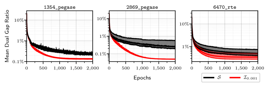
Figure 1: Convergence of the mean dual gap ratio on testing set samples during training.

The DCOPF instances are first converted to the normal form

$$\min_{\mathbf{x}}\quad \mathbf{c}^{\top}\mathbf{x}$$ (19a)

s.t. $$\mathbf{A}\mathbf{x}=\mathbf{b}_{\beta}$$ (19b)

$$\mathbf{l}\leq\mathbf{x}\leq\mathbf{u}$$ (19c)

Since only the loads vary, $\mathbf{A}$, $\mathbf{c}$, $\mathbf{l}$, and $\mathbf{u}$ stay constant from instance to instance, while $\mathbf{b}$ varies. Thus, the neural network takes $\mathbf{b}$ as input and outputs $\mathbf{y}$, both of which are of size $m$.

For the purposes of reporting results only, each of the problems (19) is solved using Mosek 10.1.24 MOSEK ApS (2022) to obtain the optimal dual solution $\mathbf{y}^{*}$.

6.2 Results

To evaluate the performance of the proposed approaches, the dual gap of the predicted dual solution $\dot{\mathbf{y}}$ compared to the optimal dual solution $\mathbf{y}^{*}$ found by Mosek is reported. For both DSL and DIPL, the expression used for reporting the dual objective is $\mathcal{L}_{s}(\dot{\mathbf{y}})$, as defined by (7) (equivalently, following Algorithm 4 then using (3a)). As mentioned earlier, Lemma 1 guarantees that for a given $\dot{\mathbf{y}}$, $\mathcal{L}_{s}(\dot{\mathbf{y}})$ gives the tightest dual bound.

The dual gap ratio is reported as a percentage:

$$\text{Dual Gap Ratio}=\frac{\mathcal{L}(\mathbf{y}^{*})-\mathcal{L}({\dot{\mathbf{y}}})}{\mathcal{L}(\mathbf{y}^{*})}\times 100\%$$

Since the methods evaluated always produce dual-feasible solutions, the difference between the true optimal objective value and the objective value obtained from using the predictions is always non-negative.

Table 2: Dual gap ratio statistics across the testing set for each benchmark.

Benchmark	Method	Minimum	Geometric Mean	$99^{\text{th}}$ Percentile	Maximum
1354_pegase	$\mathcal{S}$	$0.14\%{\scriptstyle(\pm.014\%)}$	$0.23\%{\scriptstyle(\pm.016\%)}$	$2.15\%{\scriptstyle(\pm.030\%)}$	$13.76\%{\scriptstyle(\pm.015\%)}$
	$\mathcal{I}_{0.001}$	$0.01\%{\scriptstyle(\pm.001\%)}$	$0.14\%{\scriptstyle(\pm.004\%)}$	$2.14\%{\scriptstyle(\pm.010\%)}$	$13.82\%{\scriptstyle(\pm.007\%)}$
2869_pegase	$\mathcal{S}$	$0.15\%{\scriptstyle(\pm.018\%)}$	$0.25\%{\scriptstyle(\pm.106\%)}$	$3.73\%{\scriptstyle(\pm.194\%)}$	$10.26\%{\scriptstyle(\pm.513\%)}$
	$\mathcal{I}_{0.001}$	$0.004\%{\scriptstyle(\pm.001\%)}$	$0.05\%{\scriptstyle(\pm.001\%)}$	$3.56\%{\scriptstyle(\pm.018\%)}$	$9.96\%{\scriptstyle(\pm.002\%)}$
6470_rte	$\mathcal{S}$	$0.15\%{\scriptstyle(\pm.013\%)}$	$0.50\%{\scriptstyle(\pm.146\%)}$	$1.96\%{\scriptstyle(\pm.615\%)}$	$6.95\%{\scriptstyle(\pm.633\%)}$
	$\mathcal{I}_{0.001}$	$0.02\%{\scriptstyle(\pm.010\%)}$	$0.34\%{\scriptstyle(\pm.111\%)}$	$1.84\%{\scriptstyle(\pm.596\%)}$	$6.85\%{\scriptstyle(\pm.613\%)}$

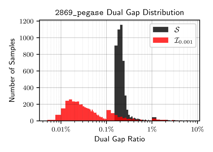
Figure 2: Distribution of dual gap ratios over testing set samples for the 2869_pegase benchmark.

Figure 1 shows the convergence of the mean dual gap ratio on the testing set compared to the optimal solution across 10 trials on the 1354_pegase, 2869_pegase, and 6470_rte benchmarks. The area between the best and worst seed is shaded in. These figures clearly show the benefits of DIPL ($\mathcal{I}_{0.001}$) over DSL ($\mathcal{S}$). This is especially visible on the 2869_pegase test case, where DIPL brings improvements to the mean dual gap ratio that are close to an order of magnitude. Observe also the low variances of DIPL on these test cases – this shows that DIPL is more robust to different choices of initial learning model weights and training/validation splits. Table 2 shows the minimum, geometric mean, $99^{\text{th}}$ percentile, and maximum dual gap ratio over the testing set samples. Each entry in the table is the geometric mean $\pm$ the standard deviation over the ten trials. Overall, DIPL produces mean optimality gaps in the range $[0.05,0.34]\%$, while DSL produces mean optimality gaps in the range of $[0.25,0.5]\%$. Remarkably, the smallest duality gaps of DIPL are in the range $[0.004,0.02]\%$. Figure 2, 3 and 4 show the distribution of the dual gap ratios over the testing set samples, averaged across the ten trials. These figures show that, although there are a few outliers, the vast majority of the testing instances has a dual gap ratio under $0.5\%$ for DIPL and certainly under $1.0\%$ for both DSL and DIPL. In summary, these results show that DSL and DIPL are both capable of producing dual-feasible solutions with extremely tight dual bounds for large-scale DCOPF problems.

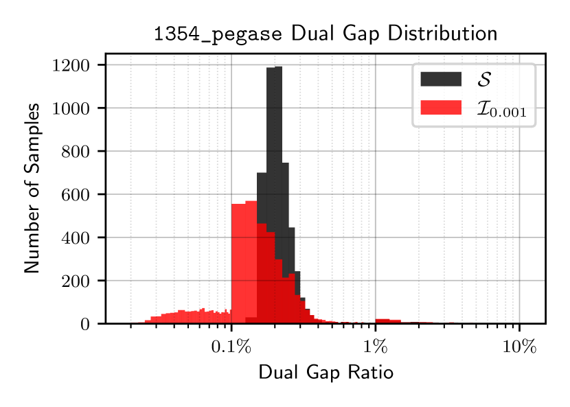
Figure 3: Distribution of dual gap ratios over testing set samples for the 1354_pegase benchmark.

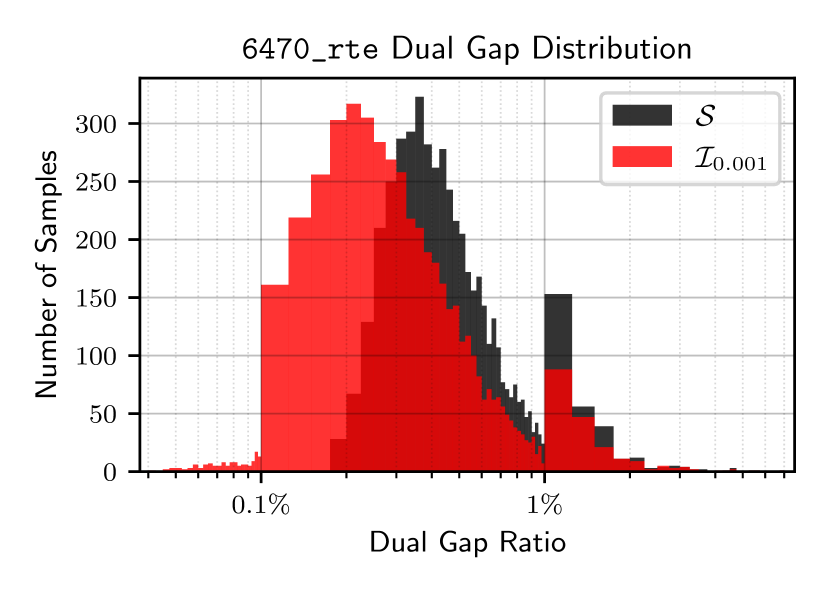
Figure 4: Distribution of dual gap ratios over testing set samples for the 6470_rte benchmark.

7 Conclusion

This paper presents DSL and DIPL, two self-supervised learning methods to learn dual-feasible solutions to parametric linear programs with bounded variables. The methods are each based on a corresponding dual ascent optimization algorithm. Both DSL and DIPL guarantee dual feasibility by predicting the dual variables associated with the main constraints and recovering the duals of the bound constraints in a closed form. To the authors’ knowledge, DIPL is the first implementation of dual interior-point gradient algorithm for machine learning. DIPL improves on DSL by considering the barrier formulation of the dual, a smoother problem that is more amenable to learning. Importantly, the paper provides closed-form expressions to recover the tightest dual values associated with the bound constraints and to compute the gradient of the loss function with respect the core duals. DSL and DIPL were evaluated on large-scale, industrial-size optimal power flow problems, and shows that they both produce high-fidelity dual-feasible solutions providing tight valid dual bounds. Both achieve a mean optimality gap under $0.5\%$ on the largest test case. Moreover, DIPL consistently outperforms DSL, achieving gaps as low as $0.004\%$ on some test cases and demonstrating the benefits of its smoother, barrier-based formulation.

Future work is needed to understand the characteristics of the few outliers in the testing set which have a relatively high maximum error, and to upgrade the algorithms and training steps to address them. In addition, it is important to evaluate DIPL and DSL on other formulations, such as the security-constrained economic dispatch formulations that feature reserve constraints. These formulations are used in practice to clear the real-time market every five minutes.

8 Acknowledgements

This research was partly supported by NSF award 2112533 and ARPA-E PERFORM award AR0001136. Experiments were run on the PACE Phoenix cluster PACE (2017).

Appendix A Missing Proofs

Lemma 1.

The optimal solution to the inner problem $\Xi(\hat{\mathbf{y}})$ is given by

$$\hat{\mathbf{z}}^{l} =|\mathbf{c}-\mathbf{A}^{\top}\hat{\mathbf{y}}|^{+}$$

$$\hat{\mathbf{z}}^{u} =|\mathbf{c}-\mathbf{A}^{\top}\hat{\mathbf{y}}|^{-}$$

In addition, the tuple $(\hat{\mathbf{y}},\,\hat{\mathbf{z}}^{l},\,\hat{\mathbf{z}}^{u})$ is a feasible solution to Problem (3).

Proof.

Let $\hat{\mathbf{z}}=\mathbf{c}-\mathbf{A}^{\top}\hat{\mathbf{y}}$. The inner problem $\Xi(\hat{\mathbf{y}})$ now reads:

$$\Xi(\hat{\mathbf{y}})=\max_{\mathbf{z}^{l},\,\mathbf{z}^{u}}\quad \mathbf{l}^{\top}\mathbf{z}^{l}-\mathbf{u}^{\top}\mathbf{z}^{u}$$

s.t. $$\mathbf{z}^{l}-\mathbf{z}^{u}=\hat{\mathbf{z}}$$

$$\mathbf{z}^{l},\,\mathbf{z}^{u}\geq 0$$

Any $\mathbf{z}^{l},\,\mathbf{z}^{u}\geq 0$ that satisfy $\mathbf{z}^{l}-\mathbf{z}^{u}=\hat{\mathbf{z}}$ are feasible to $\Xi(\hat{\mathbf{y}})$ and thus Problem (3) as well. Since $\mathbf{l}<\mathbf{u}$, the objective value is maximized when $\mathbf{z}^{u}$ is as low as possible. This problem can be solved analytically by considering the sign of $\hat{\mathbf{z}}_{i}$:

1. $\hat{\mathbf{z}}_{i}>0\implies\mathbf{z}^{l}_{i}>\mathbf{z}^{u}_{i}\implies\mathbf{z}^{l}_{i}>0$. To maximize the objective, the optimal solution sets $\mathbf{z}^{u}_{i}=0$ and recovers $\mathbf{z}^{l}_{i}=\hat{\mathbf{z}}_{i}$.

2. $\hat{\mathbf{z}}_{i}=0\implies\mathbf{z}^{l}_{i}=\mathbf{z}^{u}_{i}$. To maximize the objective, the optimal solution sets $\mathbf{z}^{u}_{i}=0$ and recovers $\mathbf{z}^{l}_{i}=0$.

3. $\hat{\mathbf{z}}_{i}<0\implies\mathbf{z}^{l}_{i}<\mathbf{z}^{u}_{i}\implies\mathbf{z}^{u}_{i}>0$. In this case, $\mathbf{z}^{u}_{i}$ cannot be set to 0 since $\mathbf{z}^{l}_{i}-\mathbf{z}^{u}_{i}$ must be negative. Still, $\mathbf{z}^{u}_{i}$ should be as low as possible – the optimal solution sets $\mathbf{z}^{u}_{i}=-\hat{\mathbf{z}}_{i}$ and recovers $\mathbf{z}^{l}_{i}=0$.

Thus the optimal solution to the inner problem is given by:

$$\hat{\mathbf{z}}^{l}_{i} =\begin{cases}\hat{\mathbf{z}}_{i}&\hskip 7.39772pt\text{if }\hat{\mathbf{z}}_{i}\geq 0\\ 0&\hskip 7.39772pt\text{if }\hat{\mathbf{z}}_{i}<0\end{cases}=|\hat{\mathbf{z}}|^{+}$$

$$\hat{\mathbf{z}}^{u}_{i} =\begin{cases}0&\text{if }\hat{\mathbf{z}}_{i}\geq 0\\ -\hat{\mathbf{z}}_{i}&\text{if }\hat{\mathbf{z}}_{i}<0\end{cases}=|\hat{\mathbf{z}}_{i}|^{-}$$

∎

Lemma 2.

The optimal solution to the inner problem $\Psi_{\mu}(\tilde{\mathbf{y}})$ (12) is given by

$$\tilde{\mathbf{z}}_{l} =\frac{2\mu+(\mathbf{u}-\mathbf{l})\odot\tilde{\mathbf{z}}+\sqrt{4\mu^{2}+(\mathbf{u}-\mathbf{l})^{2}\odot\tilde{\mathbf{z}}^{2}}}{2(\mathbf{u}-\mathbf{l})}$$

$$\tilde{\mathbf{z}}_{u} =\frac{2\mu-(\mathbf{u}-\mathbf{l})\odot\tilde{\mathbf{z}}+\sqrt{4\mu^{2}+(\mathbf{u}-\mathbf{l})^{2}\odot\tilde{\mathbf{z}}^{2}}}{2(\mathbf{u}-\mathbf{l})}$$

where $\tilde{\mathbf{z}}\,{=}\,\mathbf{c}{-}\mathbf{A}^{\top}\tilde{\mathbf{y}}$. In addition, $(\tilde{\mathbf{y}},\,\tilde{\mathbf{z}}^{l},\,\tilde{\mathbf{z}}^{u})$ is a feasible solution to Problems (3) and (10).

Proof.

Problem (12) is strictly convex, hence, it has a unique optimal solution. In addition, this optimal solution satisfies the KKT equations

$$\mathbf{z}^{l}-\mathbf{z}^{u} =\mathbf{c}-\mathbf{A}^{\top}\tilde{\mathbf{y}}$$

$$(\mathbf{x}-\mathbf{l})\odot\mathbf{z}^{l} =\mu\mathbf{e}$$

$$(\mathbf{u}-\mathbf{x})\odot\mathbf{z}^{u} =\mu\mathbf{e}$$

$$\mathbf{l}\leq\mathbf{x}\leq\mathbf{u}$$

$$\mathbf{z}^{l},\,\mathbf{z}^{u}\geq 0$$

where $\mathbf{e}$ is a vector of all ones. Define $\tilde{\mathbf{z}}=\mathbf{c}-\mathbf{A}^{\top}\tilde{\mathbf{y}}$. Eliminating $\mathbf{z}^{l}=\tilde{\mathbf{z}}+\mathbf{z}^{u}$ and $\mathbf{x}=\mathbf{u}-\frac{\mu}{\mathbf{z}^{u}}$ yields

$$\mathbf{z}^{l} =\tilde{\mathbf{z}}+\mathbf{z}^{u}$$

$$\mathbf{x} =\mathbf{u}-\frac{\mu}{\mathbf{z}^{u}}$$

$$(\mathbf{u}-\mathbf{l}-\frac{\mu}{\mathbf{z}^{u}})\odot(\tilde{\mathbf{z}}+\mathbf{z}^{u}) =\mu\mathbf{e}$$

Since $\mathbf{z}^{u}>0$ in any optimal solution, multiplying the last equation by $\mathbf{z}^{u}$ yields a quadratic equation in $\mathbf{z}^{u}$

$$\big{(}\mathbf{z}^{u}\odot(\mathbf{u}-\mathbf{l})-\mu\mathbf{e}\big{)}\odot(\tilde{\mathbf{z}}+\mathbf{z}^{u}) =\mu\mathbf{z}^{u},$$

which decomposes into $n$ quadratic equations

$$(\mathbf{u}_{i}-\mathbf{l}_{i})(\mathbf{z}^{u}_{i})^{2}+\big{(}\tilde{\mathbf{z}}_{i}(\mathbf{u}_{i}-\mathbf{l}_{i})-2\mu\big{)}\mathbf{z}^{u}_{i}-\mu\tilde{\mathbf{z}}_{i} =0,\ \forall i.$$

Using the quadratic formula yields

$$(\tilde{\mathbf{z}}^{u}_{i})^{\pm}=\frac{2\mu-(\mathbf{u}_{i}-\mathbf{l}_{i})z\pm\sqrt{4\mu^{2}+(\mathbf{u}_{i}-\mathbf{l}_{i})^{2}\tilde{\mathbf{z}}_{i}^{2}}}{2(\mathbf{u}_{i}-\mathbf{l}_{i})}$$

Following the same procedure but instead eliminating $\mathbf{z}^{u}$ yields

$$(\tilde{\mathbf{z}}^{l}_{i})^{\pm}=\frac{2\mu+(\mathbf{u}_{i}-\mathbf{l}_{i})\tilde{\mathbf{z}}_{i}\pm\sqrt{4\mu^{2}+(\mathbf{u}_{i}-\mathbf{l}_{i})^{2}\tilde{\mathbf{z}}_{i}^{2}}}{2(\mathbf{u}_{i}-\mathbf{l}_{i})}$$

Recall that $\mathbf{z}^{l},\,\mathbf{z}^{u}>0$ in any dual-feasible solution (because of the log term). If $\tilde{\mathbf{z}}_{i}\geq 0$, then $(\tilde{\mathbf{z}}^{l}_{i})^{-}\leq 0$. Likewise, if $\tilde{\mathbf{z}}_{i}\leq 0$, then $(\tilde{\mathbf{z}}^{u}_{i})^{-}\leq 0$. Therefore, the only valid solution is $(\tilde{\mathbf{z}}^{l})^{+},\,(\tilde{\mathbf{z}}^{u})^{+}$.

This yields $\tilde{\mathbf{z}}^{l}\,{=}\,(\mathbf{z}^{l})^{+}$ and $\tilde{\mathbf{z}}^{u}\,{=}\,(\mathbf{z}^{u})^{+}$. By construction, $\tilde{\mathbf{z}}^{l},\tilde{\mathbf{z}}^{u}\,{>}\,0$ and $\mathbf{A}^{\top}\tilde{\mathbf{y}}\,{+}\,\tilde{\mathbf{z}}^{l}\,{-}\,\tilde{\mathbf{z}}^{u}\,{=}\,\mathbf{c}$. Thus, $(\tilde{\mathbf{y}},\tilde{\mathbf{z}}^{l},\tilde{\mathbf{z}}^{u})$ is feasible for Problems (3) and (10). ∎

Lemma 3.

The gradient of $\mathcal{L}_{\mu}(\tilde{\mathbf{y}})$ with respect to $\tilde{\mathbf{y}}$ is given by

$$\nabla_{\tilde{\mathbf{y}}}\,\mathcal{L}_{\mu}(\tilde{\mathbf{y}})=\mathbf{b}-\mathbf{A}\tilde{\mathbf{x}}$$

where $\tilde{\mathbf{z}}=\mathbf{c}-\mathbf{A}^{\top}\tilde{\mathbf{y}}$ and

$$\tilde{\mathbf{x}}_{i}=\begin{cases}\frac{2\mu+(\mathbf{u}_{i}+\mathbf{l}_{i})\tilde{\mathbf{z}}_{i}-\sqrt{4\mu^{2}+(\mathbf{u}_{i}-\mathbf{l}_{i})^{2}\tilde{\mathbf{z}}_{i}^{2}}}{2\tilde{\mathbf{z}}_{i}}&\text{if $\tilde{\mathbf{z}}_{i}\neq 0$}\\ (\mathbf{u}_{i}+\mathbf{l}_{i})/{2}&\text{if $\tilde{\mathbf{z}}_{i}=0$}\end{cases}$$

Proof.

Problem (12) is strictly convex, hence, it has a unique optimal solution. In addition, this optimal solution satisfies the KKT equations

$$\mathbf{z}^{l}-\mathbf{z}^{u} =\mathbf{c}-\mathbf{A}^{\top}\tilde{\mathbf{y}}$$

$$(\mathbf{x}-\mathbf{l})\odot\mathbf{z}^{l} =\mu\mathbf{e}$$

$$(\mathbf{u}-\mathbf{x})\odot\mathbf{z}^{u} =\mu\mathbf{e}$$

$$\mathbf{l}\leq\mathbf{x}\leq\mathbf{u}$$

$$\mathbf{z}^{l},\,\mathbf{z}^{u}\geq 0$$

where $\mathbf{e}$ is a vector of all ones. Define $\tilde{\mathbf{z}}=\mathbf{c}-\mathbf{A}^{\top}\mathbf{y}$. Eliminating $\mathbf{z}^{l}=\tilde{\mathbf{z}}+\mathbf{z}^{u}$ and $\mathbf{z}^{u}=\frac{\mu\mathbf{e}}{\mathbf{u}-\mathbf{x}}$ yields

$$\mathbf{z}^{l}=\tilde{\mathbf{z}}+\mathbf{z}^{u}$$

$$\mathbf{z}^{u}=\frac{\mu\mathbf{e}}{\mathbf{u}-\mathbf{x}}$$

$$(\mathbf{x}-\mathbf{l})\odot(\tilde{\mathbf{z}}+\frac{\mu\mathbf{e}}{\mathbf{u}-\mathbf{x}})=\mu\mathbf{e}$$

Since $\mathbf{x}<\mathbf{u}$ in any optimal solution, multiplying the last equation by $(\mathbf{u}-\mathbf{x})$ yields a quadratic equation in $\mathbf{x}$

$$(\mathbf{x}-\mathbf{l})\odot\big{(}\tilde{\mathbf{z}}\odot(\mathbf{u}-\mathbf{x})+\mu\mathbf{e}\big{)}=\mu(\mathbf{u}-\mathbf{x})$$

which decomposes into $n$ quadratic equations

$$\tilde{\mathbf{z}}_{i}\mathbf{x}_{i}^{2}-\big{(}\tilde{\mathbf{z}}_{i}(\mathbf{u}_{i}+\mathbf{l}_{i})+2\mu\big{)}\mathbf{x}_{i}+\tilde{\mathbf{z}}_{i}\mathbf{l}_{i}\mathbf{u}_{i}+\mu(\mathbf{u}_{i}+\mathbf{l}_{i})=0,\ \forall i$$

Using the quadratic formula to find the roots yields

$$\tilde{\mathbf{x}}_{i}=\frac{2\mu+\tilde{\mathbf{z}}_{i}(\mathbf{u}_{i}+\mathbf{l}_{i})-\sqrt{4\mu^{2}+\tilde{\mathbf{z}}_{i}^{2}(\mathbf{u}_{i}-\mathbf{l}_{i})^{2}}}{2\tilde{\mathbf{z}}_{i}}$$

When $\tilde{\mathbf{z}}_{i}=0$, $\lim_{\tilde{\mathbf{z}}_{i}\rightarrow 0}\mathbf{x}_{i}=(\mathbf{u}_{i}+\mathbf{l}_{i})/2$ is used instead. Thus, the optimal value for each $\mathbf{x}_{i}$ is given by

$$\tilde{\mathbf{x}}_{i}=\begin{cases}(\mathbf{u}_{i}+\mathbf{l}_{i})/{2}\quad\quad\quad\quad\enspace\text{if $\tilde{\mathbf{z}}_{i}=0$, otherwise}\\[8.53581pt] \displaystyle\frac{2\mu+(\mathbf{u}_{i}+\mathbf{l}_{i})\tilde{\mathbf{z}}_{i}-\sqrt{4\mu^{2}+(\mathbf{u}_{i}-\mathbf{l}_{i})^{2}\tilde{\mathbf{z}}_{i}^{2}}}{2\tilde{\mathbf{z}}_{i}}\end{cases}$$

Since $\tilde{\mathbf{x}}_{i}=\frac{\delta\Psi_{\mu}(\tilde{\mathbf{y}})}{\delta\tilde{\mathbf{z}}_{i}}$, the chain rule is used to find the gradient of $\Psi_{\mu}(\tilde{\mathbf{y}})$ with respect to $\tilde{\mathbf{y}}$:

$$\nabla_{\tilde{\mathbf{y}}}\,\Psi_{\mu}(\tilde{\mathbf{y}})=-\mathbf{A}\tilde{\mathbf{x}}$$

Finally, the gradient of the $\Psi$-Dual objective with respect to $\mathbf{y}$ is given by

$$\nabla_{\tilde{\mathbf{y}}}\,\Big{[}\mathbf{b}^{\top}\tilde{\mathbf{y}}+\Psi_{\mu}(\tilde{\mathbf{y}})\Big{]}=\mathbf{b}-\mathbf{A}\tilde{\mathbf{x}}$$

∎

References

• Applegate et al. (2021) Applegate, D., Díaz, M., Hinder, O., Lu, H., Lubin, M., O’Donoghue, B., and Schudy, W. Practical large-scale linear programming using primal-dual hybrid gradient. Advances in Neural Information Processing Systems, 34:20243–20257, 2021. URL https://doi.org/10.48550/arXiv.2106.04756.
• Babaeinejadsarookolaee et al. (2019) Babaeinejadsarookolaee, S. et al. The Power Grid Library for Benchmarking AC Optimal Power Flow Algorithms. Technical report, IEEE PES PGLib-OPF Task Force, 2019. URL https://doi.org/10.48550/arXiv.1908.02788.
• Boyd & Mutapcic (2006) Boyd, S. and Mutapcic, A. Subgradient methods. Notes of EE364b, Stanford University, Winter Quarter, 2006. URL https://see.stanford.edu/materials/lsocoee364b/02-subgrad_method_notes.pdf.
• Chen et al. (2023) Chen, W., Tanneau, M., and Hentenryck, P. V. End-to-end feasible optimization proxies for large-scale economic dispatch. CoRR, abs/2304.11726, 2023. URL https://doi.org/10.48550/arXiv.2304.11726.
• Donti et al. (2021) Donti, P. L., Rolnick, D., and Kolter, J. Z. DC3: A learning method for optimization with hard constraints. In 9th International Conference on Learning Representations, ICLR 2021, Virtual Event, Austria, May 3-7, 2021, 2021. URL https://iclr.cc/virtual/2021/poster/2868.
• Fioretto et al. (2020) Fioretto, F., Mak, T. W., and Van Hentenryck, P. Predicting AC Optimal Power Flows: Combining deep learning and lagrangian dual methods. In Proceedings of the AAAI conference on artificial intelligence, volume 34, pp.  630–637, 2020. URL https://doi.org/10.1609/aaai.v34i01.5403.
• Kingma & Ba (2015) Kingma, D. and Ba, J. Adam: A method for stochastic optimization. In International Conference on Learning Representations (ICLR), San Diega, CA, USA, 2015. URL https://doi.org/10.48550/arXiv.1412.6980.
• MOSEK ApS (2022) MOSEK ApS. MOSEK Optimizer API for Julia 10.1.24, 2022. URL https://docs.mosek.com/latest/juliaapi/index.html.
• Nesterov (2005) Nesterov, Y. Smooth minimization of non-smooth functions. Mathematical programming, 103:127–152, 2005. URL https://doi.org/10.1007/s10107-004-0552-5.
• PACE (2017) PACE. Partnership for an Advanced Computing Environment (PACE), 2017. URL http://www.pace.gatech.edu.
• Park & Van Hentenryck (2023) Park, S. and Van Hentenryck, P. Self-supervised primal-dual learning for constrained optimization. Proceedings of the AAAI Conference on Artificial Intelligence, 37(4):4052–4060, Jun. 2023. URL https://doi.org/10.1609/aaai.v37i4.25520.
• Paszke et al. (2019) Paszke, A. et al. PyTorch: An Imperative Style, High-Performance Deep Learning Library. In Wallach, H., Larochelle, H., Beygelzimer, A., d’Alché Buc, F., Fox, E., and Garnett, R. (eds.), Advances in Neural Information Processing Systems 32, pp.  8024–8035. Curran Associates, Inc., 2019. URL https://doi.org/10.48550/arXiv.1912.01703.
• Qian et al. (2023) Qian, C., Chételat, D., and Morris, C. Exploring the power of graph neural networks in solving linear optimization problems. arXiv preprint arXiv:2310.10603, 2023. URL https://doi.org/10.48550/arXiv.2310.10603.
• Qiu et al. (2023) Qiu, G., Tanneau, M., and Van Hentenryck, P. Dual Conic Proxies for AC Optimal Power Flow. arXiv preprint arXiv:2310.02969, 2023. URL https://doi.org/10.48550/arXiv.2310.02969.
• Shor et al. (2012) Shor, N., Kiwiel, K., and Ruszczynski, A. Minimization Methods for Non-Differentiable Functions. Springer Series in Computational Mathematics. Springer Berlin Heidelberg, 2012. ISBN 9783642821189. URL https://doi.org/10.1007/978-3-642-82118-9.
• Tianyi Lin & Zhang (2021) Tianyi Lin, Shiqian Ma, Y. Y. and Zhang, S. An admm-based interior-point method for large-scale linear programming. Optimization Methods and Software, 36(2-3):389–424, 2021. URL https://doi.org/10.1080/10556788.2020.1821200.