Analog model of Kerr black holes in scalar-tensor theories using binary Bose-Einstein condensates:
Quasibound states and tachyonic instabilities

Abstract

We propose an analog model of the Kerr black hole in scalar-tensor theories using 2-component Bose-Einstein Condensates. We focus on two types of gapped excitations induced by the modes of two-component condensates with a relative phase of $0$ and $\pi$, analogous to the massive scalar field with positive and negative mass squared, respectively. The inclusion of space-dependent Rabi coupling can induce an effective space-dependent mass term. We study superradiant instabilities resulting from the quasibound states corresponding to positive mass squared and the tachyonic instabilities arising from negative mass squared in both frequency and time domains. These instabilities resemble two possible mechanisms that make Kerr black holes unstable in scalar-tensor gravity with the presence of matter around the black hole. Our proposed analog gravity model could potentially be implemented in future experiments, drawing from the success of recent analog rotating black hole implementations.

I INTRODUCTION

Analog gravity can be traced back to the pioneering work by Unruh [1]. The idea is to use the sound waves in a moving fluid as an analog to light waves in curved spacetime and further show that supersonic fluid can generate a “dumb hole”, an acoustic analog of a black hole. Since its development, the analog gravity program has received much attention for exploring fundamental physics through interdisciplinary research among particle/astro physicists and condensed matter physicists (for a review see [2]).

The linear perturbations around a perturbed black hole can be probed through its damped oscillatory behavior in the form of so-called quasinormal modes (QNMs) [3, 4, 5]. The QNMs have a complex frequency where its real part gives the frequency of oscillations and the imaginary part determines the lifetime. During the ringdown phase of a perturbed black hole, possibly formed from a binary black hole merger, the observed spectrum of QNMs encodes information such as the angular momentum and mass of a black hole. Importantly, this encoding is independent of the initial conditions of perturbations, which allows for testing both general relativity and alternative theories of relativity [6]. In particular, recent studies have focused on mimicking the geometry of a spinning black hole in 1+2 dimensions using a draining bathtub vortex flow [7, 8, 9, 10]. An analog model of rotating black holes has also been proposed in the photon fluid [11, 12, 13]. With the state-of-the-art experimental technology of Bose-Einstein condensates (BECs), the first successful experiment of Hawking radiation and its time dependence in a single-component BEC system in 1+1 dimensions is implemented in [14, 15]. Subsequently, a theoretical extension to binary BECs in 1+1 dimensions has been put forward as an analog model to simulate the behavior of the massive scalar field in the early universe and black holes [16, 17, 18, 19, 20, 21]. A further extension to 1+2 dimensions provides a fantastic platform to study quantum vortex instabilities in the background of analogous rotating black holes [22, 23].

The most studied alternatives to general relativity are scalar-tensor theories [24]. Recent studies in [25, 26, 27] have revealed the mechanism that renders Kerr black holes unstable due to the presence of matter in the vicinity of the black holes, which alters the QNMs spectrum. One of the mechanisms involves positive mass squared due to the existence of so-called quasibound states, leading to superradiant instabilities when the spin of a black hole exceeds certain threshold. The other comes from negative mass squared, causing tachyonic instabilities that may further trigger the development of black-hole hairs, known as ”spontaneous scalarization”.

In this Letter, we propose an analog model of Kerr black holes in scalar-tensor theories using binary BEC systems. Introducing Rabi transition between two atomic hyperfine states, the system can be represented by a coupled two-field model that involves both gapless excitations and gapped excitations [16, 17, 18, 19, 20]. The advent of experimental studies on the tunable binary BECs in [28, 29, 30, 31] makes it possible to observe these two types of excitations. We primarily focus on the gapped modes, which are analogous to the massive scalar field. In the background of zero and $\pi$ phase difference between two-component condensates, the induced mass term can be positive and negative, respectively [32, 33, 34]. Subsequently, the space-dependent Rabi coherent coupling [31, 35, 36, 37] can generate the spatially dependent mass term, allowing for the simulation of superradiant and tachyonic instabilities in the background of a draining vortex flow with an analogous geometry of rotating black holes.

II FORMALISM

We consider tunable binary BECs with identical atoms in two distinct internal hyperfine states. Experimentally, one can tune the values of scattering length using Feshbach resonances, such as those associated with the two hyperfine states of ${}^{87}\text{Rb}$ [38, 39, 40, 41]. Additionally, we introduce the Rabi transition between these states with the strength determined by the Rabi-frequency $\Omega$, where $\Omega\geq 0$. With the unit $\hbar=1$ throughout this paper, the coupled time-dependent equations of motion in $1+2$ dimensions are expressed by

$$i\partial_{t}\hat{\Psi}_{i}=\left[-\frac{1}{2m_{a}}\nabla^{2}+V_{i}+g_{ii}\hat{\Psi}_{i}^{\dagger}\hat{\Psi}_{i}+g_{ij}\hat{\Psi}_{j}^{\dagger}\hat{\Psi}_{j}\right]\hat{\Psi}_{i}-\frac{\Omega}{2}\hat{\Psi}_{j}\,$$ (1)

with $i\neq j$ and $i,j=1,2$. $m_{a}$ represents atomic mass and $V_{i}$ denotes the external potentials on the hyperfine states $i$. Furthermore, $g_{ii},g_{ij}$ give the interaction strengths of atoms between the same hyperfine states and different hyperfine states, respectively. The coupling strengths are related to the scattering lengths. The condensate wavefunctions are given by the expectation value of the field operator $\langle\hat{\Psi}_{i}\rangle$  , $\langle\hat{\Psi}_{i}\rangle(\mathbf{r},t)=\sqrt{\rho_{i}(\mathbf{r},t)}\,e^{i\theta_{i}(\mathbf{r},t)-i\mu t}$ with the chemical potential $\mu$. The condensate flow velocities are given by $\mathbf{v}_{i}={\gradient}\theta_{i}/m_{a}$. The equations for $\rho_{i}$ and $\theta_{i}$ of the condensate wavefunctions can be found in [18, 17, 19]. The perturbations around the stationary wavefunctions are defined through $\hat{\Psi}_{i}=\langle\hat{\Psi}_{i}\rangle(1+\hat{\phi}_{i})\,,$ where the fluctuation fields decompose in terms of the density and the phase as $\hat{\phi}_{i}=\delta{\hat{n}_{i}}+i\delta\hat{\theta}_{i}=\frac{\delta\hat{\rho}_{i}}{2\rho_{i}}+i\delta\hat{\theta}_{i}\,.$ According to [18], one can decouple the equations for the general spatially dependent condensate wavefunctions and the coupling strengths by choosing the time-independent background solutions $\rho_{1}=\rho_{2}=\rho$, $\theta_{1}=\theta_{2}=\theta$ or $\theta_{1}=\theta,\theta_{2}=\theta\pm\pi$, and $g_{11}=g_{22}=g$ (See Supplements) [32, 34]. The chosen scattering parameters of $g_{12}<g$ in the binary systems can result in a miscible state of the background condensates [28, 29, 30, 31].

The decoupled equations are shown in [18, 17, 19] in terms of the (gapless) density and (gapped) spin modes given by $\sqrt{2}\delta\hat{n}_{d/s}=\delta\hat{n}_{1}\pm\delta\hat{n}_{2}$ and $\sqrt{2}\delta\hat{\theta}_{d/s}=\delta\hat{\theta}_{1}\pm\delta\hat{\theta}_{2}$. Combining them yields a single equation for $\delta\hat{\theta}_{s}$ in the form of the Klein-Gordon equation for a massive scalar field,

$$\frac{1}{\sqrt{-\mathbf{g}}}\partial_{\mu}\left(\sqrt{-\mathbf{g}}\,\mathbf{g}^{\mu\nu}\partial_{\nu}\delta\hat{\theta}_{s}\right)-m_{\text{eff}}^{2}\delta\hat{\theta}_{s}=0,$$ (2)

where the spatial dependent sound speed is given by $c^{2}=[(g-g_{12})\rho\pm\Omega]/m_{a}$, and the effective mass by $m^{2}_{\text{eff}}=\pm 2m_{a}^{2}c\,\Omega/\rho$, with the $"+"$ sign corresponding to the zero-phase difference and the $"-"$ sign to the $\pi$-phase difference. The acoustic metric $\mathbf{g}^{\mu\nu}$ depends on the background $\rho$ and $\theta$. Following [23], to mimic the geometry of a rotating black hole, we consider the draining vortex with the velocity flow

$$\mathbf{v}=\frac{1}{m_{a}}{\gradient}\theta=\frac{-d\mathbf{e}_{r}+\ell\mathbf{e}_{\phi}}{m_{a}r}=v_{r}\mathbf{e}_{r}+v_{\phi}\mathbf{e}_{\phi},$$ (3)

where the winding number $\ell$ is taken as an integer (hereafter $\ell=1$) for quantum vortices and $d>0$ for the draining flow. In the Thomas-Fermi approximations, the region of interest is far from the core of the vortex with the radius $r\gg R_{\text{TF}}=\sqrt{\frac{d^{2}+l^{2}}{2m_{a}\rho_{\infty}(g+g_{12})}}$, where the density $\rho$ can be treated as a constant, $\rho\simeq\rho_{\infty}$ given by $\rho_{\infty}=\frac{1}{g+g_{12}}\left(\mu-V_{0}\pm\frac{\Omega}{2}\right)$ for an uniform external potential $V_{0}$. The details can be seen in Supplements. Using the coordinate transformations $d\tilde{t}=dt-(c^{2}/v_{r}^{2}-1)^{-1}dr,$ $d\tilde{\phi}=d\phi-\frac{v_{r}v_{\phi}}{r(c^{2}-v_{r}^{2})}dr,$ the metric becomes

$$ds^{2}=\tilde{g}_{\mu\nu}^{\text{vortex}}d\tilde{x}^{\mu}d\tilde{x}^{\nu}$$

$$\propto-\left(1-\frac{r_{E}^{2}}{r^{2}}\right)d\tilde{t}^{2}+\left(1-\frac{r^{2}_{H}}{r^{2}}\right)^{-1}dr^{2}-\frac{2\ell}{m_{a}}\,d\tilde{\phi}d\tilde{t}+r^{2}d\tilde{\phi}^{2}\,$$ (4)

with $\tilde{x}=(\tilde{t},r,\tilde{\phi})$. Apparently, the acoustic horizon and the ergosphere are located at $r_{\text{H}}=d/m_{a}c$ and $r_{\text{E}}=\sqrt{d^{2}+\ell^{2}}/m_{a}c$, respectively. Hereafter, we simplify the formula by defining dimensionless variables as $r/r_{H}\rightarrow r$, $c\,\tilde{t}/r_{H}\rightarrow{t}$ and $r_{H}\Omega/c\rightarrow\Omega$. Let us now provide the order-of-magnitude of the relevant parameters from the experiment. In the case of Rubidium atoms with a mass $m_{a}\sim 10^{-25}\text{kg}$ and a scattering length $a\sim 6\text{nm}$, the density $\rho_{\infty}$ can be prepared as much as $\sim 10^{25}\text{m}^{-3}$, giving the healing length and $R_{\text{TF}}$ such as $\xi\sim R_{\text{TH}}\sim 10^{2}\text{nm}$. Considering $r_{\text{H}}\sim 10\xi$, from $v_{r}=c$, the value of $d$ is about $d\sim 1$. Also, the measuring time to trace the evolution of the perturbed fields will be limited by the lifetime of the condensates, say $\sim 1\text{s}$, giving the dimensionless time of order ${t}\sim 10^{3}$. Using the phase fluctuation field of the form $\delta\theta_{s}({t},r,\tilde{\phi})=\frac{H_{m}(r,{t})}{\sqrt{r}}\exp\left(im\tilde{\phi}\right)$ in the Klein-Gordon equation, the radial equation in the tortoise coordinate $r^{\ast}=r+\frac{1}{2}\log{\Big{|}\frac{r-1}{r+1}\Big{|}}$ reads

$$\Bigg{\{}\frac{\partial^{2}}{\partial{r^{\ast}}^{2}}-\left(\frac{\partial}{\partial t}+i\frac{m\ell}{r^{2}}\right)^{2}-\left(\frac{r^{2}-1}{r^{2}}\right)$$

$$\times\left[\frac{1}{r^{2}}\left(m^{2}-\frac{1}{4}\right)+\frac{5}{4r^{4}}+\mu_{s}^{2}(r)\right]\Bigg{\}}H_{m}(r,t)=0$$ (5)

with $\mu^{2}_{s}(r)=\pm 2d\Omega(r)$. Further writing $H_{m}(r,t)=H_{m}(r,\omega)e^{-i\omega{t}}$ turns the time-dependent equation into the time-independent Schrodinger-like equation $\left[\partial_{r^{\ast}}^{2}+V_{\text{eff}}(r)\right]H_{m}(r,\omega)=0$ where $V_{\text{eff}}(r)=\left({\omega-\frac{m\ell}{r^{2}}}\right)^{2}-\left(\frac{r^{2}-1}{r^{2}}\right)\left[\frac{5}{4r^{4}}+\frac{1}{r^{2}}\left(m^{2}-\frac{1}{4}\right)+\mu^{2}_{s}(r)\right]$. To establish the analog gravity model of the scalar-tensor theory, the space-dependent mass term is introduced [25, 26]. The mass term due to the coupling to the surrounding matter of the black hole can be parametrized in terms of three parameters. One of them is the magnitude of the mass reflecting the coupling strength between the scalar field and matter in the scalar-tensor gravity theories, which can be controlled by the Rabi coupling $\Omega$. The other two are related to the parametrization of the mass distribution. They are the typical distance of the mass distribution $r_{0}$ from the black hole’s horizon and the distribution width $1/\alpha$. The parametrization of the distance $r_{0}$ can be attributed to the radius of the so-called innermost stable circular orbit of the particle moving around a massive object such as a black hole. The radius of the innermost circular motion depends on the mass and angular momentum (spin) of the massive object. The width of the mass distribution $1/\alpha$ is also an important parameter characterizing the surrounding matter of the black holes.

Figure 1: The comparison of the absolute value of the time-dependent profile between the cases of $\Omega_{0}=0.0$ (solid line) and $\Omega_{0}=0.4$ (dashed line) with $m=1$ (red), $m=2$ (blue), and $m=3$ while the distance is set to $r_{0}=15$. The shaded time regime indicates the echo time with $\Delta t\simeq 2r_{0}$. The inset figure shows the fundamental QNM frequency (filled circle $\rightarrow$ solid line, open circle $\rightarrow$ dashed line) obtained from frequency domain.

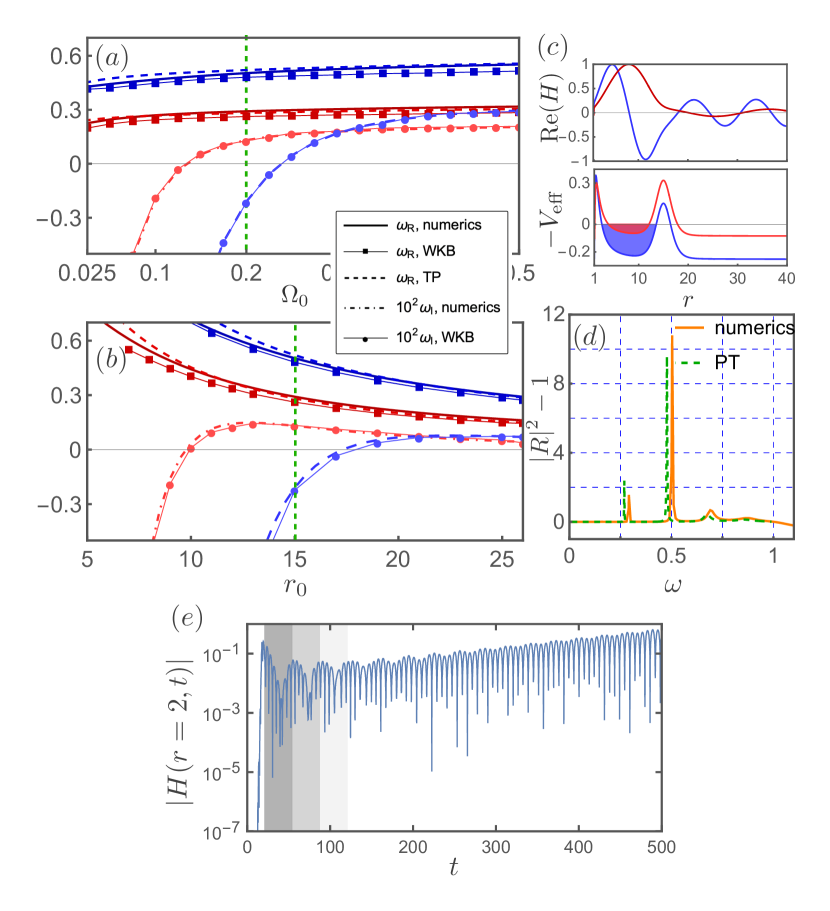
Figure 2: In the case of positive mass squared, the panel (a) shows the frequency for the mode $n=0$ (red) and $n=1$ (blue) as a function of $\Omega_{0}$ with fixed $r_{0}=15$, and the panel (b) shows the corresponding frequency as a function of $r_{0}$ with $\Omega_{0}=0.2$. (c) depicts the effective potential and the normalized radial profile for the first two modes, and (d) presents a series of peaks at the resonant frequencies in the reflection coefficient spectrum. (d) reveals the growing waveform in time domain and the echo time duration. (c)-(e) share the same values of $\Omega_{0}$ and $r_{0}$ marked in the green line in (a) and (b). Note that $m=1$, and $\alpha=1/2$ are set in all figures.

Given the boundary conditions of the pure ingoing wave $e^{-i(\omega-m\ell)r^{\ast}}$ at the horizon and the pure outgoing wave $e^{i\omega r^{\ast}}$ at infinity, the eigenfrequency of the time-independent Schrodinger-like equation can be found with the complex values $\omega=\omega_{R}+i\omega_{I}$. However, there are two types of instabilities of interest with very different dynamics on the timescale $\tau\propto 1/|\omega_{I}|$: superradiant instabilities are driven by an unstable but long-lived mode where $\omega_{R}\gg\omega_{I}$ , while tachyonic instabilities are featured with an almost pure imaginary frequency $\omega_{I}\gg\omega_{R}$ leading to a short-lived mode. In two-component BECs, the effective mass squared term can be parameterized as

$$\mu^{2}_{s}(r)=\pm 2d\Omega(r)=\pm 2d\Omega_{0}\,\text{sech}^{2}[\alpha(r-r_{0})],$$ (6)

mimicking a mass shell surrounding the black hole in the scalar-tensor gravity theory. We also present the case with the uniform mass square term for comparison in Supplements where we use the continued fraction method [42]. In the case of the spatially dependent mass term (6), we calculate the eigenfrequency numerically using the shooting method [43], where the solutions are obtained by integrating the equation from the horizon onwards and from the far distance $r$ backward with appropriate boundary conditions where they continuously vary over $r$. We also find the eigenfrequency with the generalized Pöschl-Teller (PT) semi-analytical methods [44, 45, 46]. The analytically approximated formulas for the eigenfrequency are given below. The instabilities are shown in the time domain by solving the time-dependent equation (5). For technical details, refer to Supplements.

Quasinormal modes and superradiant instabilities. In the case of the quasinormal modes, their spectrum is strongly modified by the presence of the spatially dependent mass shell, which introduces an additional barrier to the rotational barrier given by the azimuthal angular momentum $m$. The frequencies of quasinormal modes for the real and imaginary parts are found in Fig. 1, which are smaller than their counterparts without the mass shell [47, 48]. The corresponding time domain signals are obtained by solving the time-dependent equation (5) for an initial Gaussian function with reference to [49]. According to [49], small perturbations can lead to a relatively large shift of the eigenfrequency from the unperturbed one, but not to a significant change in the time domain (See an example in Supplements). Here, we present the evolution of the radial profiles, which show a significant change due to the nonzero Rabi coupling strength. The echo time (estimated from the shaded time domain around $\sim 2r_{0}$), which is the time for the radial profile to travel towards the potential barrier at $r=r_{0}$ and return to the starting position and the ringdown of the profile at late times are displayed in Fig 1. More interestingly, when $\Omega_{0}$ or $r_{0}$ reaches its respective critical value, the positive mass shell could further induce superradiant instabilities, where a local bound state is shown for the potential ($-V_{\text{eff}}$) in Fig. 2. This is similar to superradiant instabilities induced by the accretion disk around Kerr black hole in scalar-tensor gravity theories [25, 26, 27]. Let us estimate the resonance spectrum via a discrete quantization condition in the Wentzel-Kramers-Brillouin (WKB) analysis given by

$$\int_{r^{\ast}_{-}}^{r^{\ast}_{+}}dr^{\ast}\sqrt{V_{\text{eff}}(r,r_{0},\Omega_{0},\alpha)}=\left(n+\frac{1}{2}\right)\pi,\quad n=0,1,2\cdots,$$ (7)

where $r_{\pm}^{\ast}$ are the classical turning points in the effective potential $-V_{\text{eff}}$. Considering $\omega_{R}\gg|\omega_{I}|$, the condition (7) can be approximated as

$$-\frac{1}{2}\pi\sqrt{2m\ell\omega_{R}+m^{2}}+\zeta\omega_{R}+\frac{m^{2}}{2\zeta\omega_{R}}=(n+\frac{1}{2})\pi$$ (8)

as $r_{0}\gg r_{H}$ with $\zeta=r_{0}-\alpha^{-1}{\ln\left(\frac{2\sqrt{2d\Omega_{0}}}{\omega_{R}}\right)}$ and $\Omega_{0}>0$, from which $\omega\simeq\omega_{R}$ can be determined. In the limit of a thin width of the mass shell where $\alpha\rightarrow\infty$, $\zeta\rightarrow r_{0}$, the real part of the frequency becomes $\omega_{R}\sim(\frac{m}{2}+n+\frac{1}{2})\pi/r_{0}$ reducing to the known result in [50]. After plugging in the resulting frequency $\omega\simeq\omega_{R}$ in $V_{\text{eff}}$, increasing $r_{0}$ shifts the barrier away from the rotational barrier so that the shaded area in Fig. 2 decreases, giving a smaller value of $\omega_{R}$.

Nevertheless, it is noted that, for example, for $n=0$ (the fundamental mode) and $n=1$ (the overtone mode), if $r_{0}$ is above a certain value shown in Fig. 2, the imaginary part of the eigenfrequency $\omega_{I}$ becomes positive, indicating superradiant instabilities due to the existence of the so-called quasibound state. Then, as $r_{0}$ falls below the critical value, the negativeness of $\omega_{I}$ reveals the quasinormal mode. On the contrary, as $\Omega_{0}$ increases, the shaded area increases, resulting in a larger value of $\omega_{R}$. Similarly, there is a critical value of $\Omega_{0}$, above (below) which the mode suffers (becomes) superradiant instabilities (quasinormal modes). In this setup, sending a monochromatic wave into the vortex will be scattered even if the mass shell shields the vortex. If its frequency is $\omega<m\ell$, it will cause superradiant amplification, and if the frequency is also close to the spectrum frequency $\omega\sim\omega_{R}$, significant resonance amplification will occur, as shown in Fig. 2. Either a stable quasinormal mode or an unstable quasibound state is partially trapped within the mass shell and partially propagate towards spatial infinity, resembling a new class of modes in the astrophysics [26]. The instabilities associated with the quasibound states are also evident from the growth of the radial profile with time in Fig. 2. While the function $H(r=2,t)$ grows, the echo time of two neighboring peaks is about $2r_{0}$. Within the lifetime of the condensates, instabilities will destabilize the background solutions, where backreaction effects must be systematically taken into account.

Figure 3: The left panel shows the comparison among numerics, WKB and PT methods for the imaginary part of frequency as a function of $\Omega_{0}$. The right top panels depict the effective potential and the normalized radial profile for modes $n=0,1$. The right bottom panel reveals the time-dependent profile with varying $\Omega_{0}$. The parameters are fixed as $m=1,\,r_{0}=10,$ and $\alpha=1/2$.

Tachyonic instabilities. A negative mass squared could trigger tachyonic instabilities in scalar-tensor theories, which further leads to spontaneous scalarization. Tachyonic instabilities arise from a completely different mechanism than that of superradiant instabilities. It is expected that tachyonic instabilities lead to a large imaginary part with a short lifetime, namely $\omega_{I}\gg\omega_{R}$. We present numerics, PT, and WKB analytical methods to confirm the existence of the tachyonic instability spectrum in Fig. 3. A fundamental mode ($n=0$) has the largest frequency $\omega\simeq\omega_{I}$ for $\omega_{I}>0$ compared with the overtones. A larger coupling $\Omega_{0}$ and a wider shell $\alpha^{-1}$ lead to stronger tachyonic instabilities. The radial profiles $H_{m}(r,\omega)$ are also drawn for $n=0$, the fundamental mode, and $n=1$, the overtone mode, which lie within the respective classical allowed regimes. Let us assume that (7) can still be applied to give an analytical formula for the eigenfrequency with $\omega\simeq i\omega_{I}$. Substituting $\omega\simeq i\omega_{I}$ into $V_{\text{eff}}$ shows the potential profile in Fig. 3. The shaded area for the classical allowed region obeys (7) for an integer $n$ given by

$$\omega_{I}\sim\frac{1}{3}\left[\sqrt{2d\Omega_{0}}-\alpha\left(n+\frac{1}{2}\right)\right]\pi.$$ (9)

The values of $\omega_{I}$ are in good agreement with the other methods in Fig. 3. The change in $r_{0}$ may shift the potential profile horizontally but keep the shaded area almost unchanged, giving little effect to the eigenfrequencies. The value of $\Omega_{0}$ shifts the potential profile vertically, and from the analytical formulas in (9), the condition $\sqrt{2d\Omega_{0}}>\alpha(n+1/2)$ triggers tachyonic instabilities, resulting in $\omega_{I}>0$. Otherwise, the resulting $\omega_{I}<0$ indicates the quasinormal modes. The corresponding evolution of the radial profile from (5) is also displayed in the cases of the quasinormal modes for relatively small $\Omega_{0}$ and the tachyonic instabilities for relatively larger $\Omega_{0}$.

Conclusion We conclude this letter by summarizing the parameter constraints for a successful analog gravity model. The zero-phase difference between the two types of condensates give perturbed fields with positive mass squared, and the $\pi$-phase difference can give negative mass squared where the choice of one of two modes allows for experimental feasibility [32, 33]. Positive sound speed squared is required, where $g_{12}/g<1\pm\Omega_{0}/\rho g$ (with a dimension-restored variable $\Omega_{0}$), leading to a further constraint on $\Omega_{0}<\rho(g-g_{12})$ in the $\pi$-phase difference modes [51, 52]. The specific form of the mass shell function in (6) that we proposed here illustrates the analog model. The same instabilities can be observed for the general parametrization of the mass distribution by its typical distance from the black hole’s horizon and the width of the distribution. The experimentally challenging but achievable spatially dependent Rabi coupling strength has been discussed in [36].

SUPPLEMENTAL MATERIAL

Background solutions and Thomas-Fermi approximations

We show the detailed derivations of the background solutions for the density and phase of two-component BECs. Plugging in the parametrization of the condensate wavefunction of $\langle\hat{\Psi}_{i}\rangle(\mathbf{r},t)=\sqrt{\rho_{i}(\mathbf{r},t)}\,e^{i\theta_{i}(\mathbf{r},t)-i\mu_{i}t}$ to (1), the density and phase satisfy the equations given respectively by

$$i\partial_{t}\left(\sqrt{\rho_{1}}e^{i(\theta_{1}-\mu_{1}t)}\right)=\left(-\frac{1}{2m_{a}}\nabla^{2}+V_{\text{ext},1}+g_{11}\rho_{1}+g_{12}\rho_{2}\right)\sqrt{\rho_{1}}e^{i(\theta_{1}-\mu_{1}t)}-\frac{\Omega}{2}\sqrt{\rho_{2}}e^{i(\theta_{2}-\mu_{2}t)},$$ (S1)

$$i\partial_{t}\left(\sqrt{\rho_{2}}e^{i(\theta_{2}-\mu_{2}t)}\right)=\left(-\frac{1}{2m_{a}}\nabla^{2}+V_{\text{ext},2}+g_{22}\rho_{2}+g_{12}\rho_{1}\right)\sqrt{\rho_{2}}e^{i(\theta_{2}-\mu_{2}t)}-\frac{\Omega}{2}\sqrt{\rho_{1}}e^{i(\theta_{1}-\mu_{1}t)}.$$ (S2)

In the paper, we focus on the miscible regime and choose the parameters in (1) as

$$g_{11}=g_{22}\equiv g,\quad g_{12}<g,$$ (S3)

$$\mu_{1}=\mu_{2}\equiv\mu,\quad V_{1}=V_{2}\equiv V_{0}.$$ (S4)

Using the fact that

$$i\partial_{t}\left(\sqrt{\rho_{1}}e^{i(\theta_{1}-\mu_{1}t)}\right)=\left(-\frac{1}{2m_{a}}\nabla^{2}+V_{0}+g\rho_{1}+g_{12}\rho_{2}\right)\sqrt{\rho_{1}}e^{i(\theta_{1}-\mu_{1}t)}-\frac{\Omega}{2}\sqrt{\rho_{2}}e^{i(\theta_{2}-\mu_{2}t)},$$ (S5)

the left-hand side of (S5) gives

$$i\left[\partial_{t}\sqrt{\rho_{1}}+i\sqrt{\rho_{1}}(\partial_{t}\theta_{1}-\mu)\right]e^{i(\theta_{1}-\mu t)}$$ (S6)

and the right-hand side of (S5) becomes

$$\Big{\{}-\frac{1}{2m_{a}\sqrt{\rho_{1}}}\Big{[}\nabla^{2}\sqrt{\rho_{1}}+i\nabla\sqrt{\rho_{1}}\cdot\nabla\theta_{1}+i\sqrt{\rho_{1}}\nabla^{2}\theta_{1}+i\nabla\theta_{1}\cdot\left(\nabla\sqrt{\rho_{1}}+i\sqrt{\rho_{1}}\nabla\theta_{1}\right)\Big{]}$$

$$\quad\qquad V_{0}+g_{11}\rho_{1}+g_{12}\rho_{2}\Big{\}}\sqrt{\rho_{1}}e^{i(\theta_{1}-\mu t)}-\frac{1}{2}\sqrt{\rho_{2}}e^{i(\theta_{2}-\mu t)}.$$ (S7)

Therefore, Its imaginary part of (S5) leads to

$$\partial_{t}\sqrt{\rho_{1}}=\frac{\dot{\rho}_{1}}{2\sqrt{\rho_{1}}}$$

$$=-\frac{1}{2m_{a}\sqrt{\rho_{1}}}\Big{(}\nabla\sqrt{\rho_{1}}\cdot\nabla\theta_{1}+\sqrt{\rho_{1}}\nabla^{2}\theta_{1}+\nabla\theta_{1}\cdot\nabla\sqrt{\rho_{1}}\Big{)}\sqrt{\rho_{1}}-\frac{\Omega}{2}\sqrt{\rho_{2}}\sin{(\theta_{2}-\theta_{1})}$$

$$\Rightarrow$$

$$\dot{\rho}_{1}=-\frac{1}{m_{a}}\Big{(}2\nabla\sqrt{\rho_{1}}\cdot\nabla\theta_{1}+\sqrt{\rho_{1}}\nabla^{2}\theta_{1}\Big{)}\sqrt{\rho_{1}}-{\Omega}\sqrt{\rho_{1}\rho_{2}}\sin{(\theta_{2}-\theta_{1})}\,,$$ (S8a)

whereas the real part gives

$$\sqrt{\rho_{1}}(\dot{\theta}_{1}-\mu)=\frac{1}{2m_{a}}\left[\nabla^{2}\sqrt{\rho_{1}}-\sqrt{\rho_{1}}(\nabla\theta_{1})^{2}\right]-\left(V_{0}+g\rho_{1}+g_{12}\rho_{2}\right)\sqrt{\rho_{1}}$$

$$\qquad\qquad\qquad+\frac{\Omega}{2}\sqrt{\rho_{2}}\cos{(\theta_{2}-\theta_{1})}$$

$$\Rightarrow$$

$$\dot{\theta}_{1}=\frac{1}{2m_{a}\sqrt{\rho_{1}}}\left[\nabla^{2}\sqrt{\rho_{1}}-\sqrt{\rho_{1}}(\nabla\theta_{1})^{2}\right]-\left(V_{0}+g\rho_{1}+g_{12}\rho_{2}-\mu\right)+\frac{\Omega}{2}\sqrt{\frac{\rho_{2}}{\rho_{1}}}\cos{(\theta_{2}-\theta_{1})}.$$ (S8b)

Similarly, the counterpart coupled equations for the hyperfine state $2$ have the form

$$\dot{\rho}_{2}=-\frac{1}{m_{a}}\Big{(}2\nabla\sqrt{\rho_{2}}\cdot\nabla\theta_{2}+\sqrt{\rho_{2}}\nabla^{2}\theta_{2}\Big{)}\sqrt{\rho_{2}}-{\Omega}\sqrt{\rho_{1}\rho_{2}}\sin{(\theta_{1}-\theta_{2})},$$ (S9a)

$$\dot{\theta}_{2}=\frac{1}{2m\sqrt{\rho_{2}}}\left[\nabla^{2}\sqrt{\rho_{2}}-\sqrt{\rho_{2}}(\nabla\theta_{2})^{2}\right]-\left(V_{0}+g\rho_{2}+g_{12}\rho_{1}-\mu\right)+\frac{\Omega}{2}\sqrt{\frac{\rho_{1}}{\rho_{2}}}\cos{(\theta_{1}-\theta_{2})}.$$ (S9b)

The stationary solutions satisfy $\dot{\rho}=\dot{\theta}=0$ where the dot means the derivative with respect to time $t$. One would therefore immediately obtain the solutions, which are

$$\rho_{1}=\rho_{2}=\rho,\qquad\theta_{1}=\theta\,,\theta_{2}=\theta\,;\quad\quad\theta_{1}=\theta\,,\theta_{2}=\theta\pm\pi\,$$ (S10)

for zero-phase difference and $\pi$-phase difference. Imposing (S10) into (S8) and (S9) gives

$$-\frac{1}{m_{a}}\Big{(}2\nabla\sqrt{\rho}\cdot\nabla\theta+\sqrt{\rho}\nabla^{2}\theta\Big{)}\sqrt{\rho}=0$$

$$\qquad\qquad\Rightarrow-\nabla\cdot\left(\rho\frac{\nabla\theta}{m_{a}}\right)=0\Rightarrow\nabla\cdot(\rho\vec{v})=0,$$ (S11a)

$$\frac{1}{2m_{a}\sqrt{\rho}}\left[\nabla^{2}\sqrt{\rho}-\sqrt{\rho}(\nabla\theta)^{2}\right]-\left[V_{0}+(g+g_{12})\rho-\mu\right]\pm\frac{\Omega}{2}$$

$$\qquad\qquad\Rightarrow\frac{1}{2m_{a}\sqrt{\rho}}\nabla^{2}\sqrt{\rho}-\frac{m_{a}}{2}\mathbf{v}^{2}-V_{0}-(g+g_{12})\rho+\mu\pm\frac{\Omega}{2}=0,$$ (S11b)

where we have used the definition of the condensate flow velocity $\mathbf{v}=\gradient\theta/m_{a}$. The first term in (S11b) is the quantum pressure to be ignored in the hydrodynamical regime, and the plus and minus signs of the last term correspond to the solutions of zero and $\pi$ phase differences, respectively.

To solve the stationary solution, we consider the flow velocity

$$\mathbf{v}=-\frac{d}{m_{a}r}\mathbf{e}_{r}+\frac{\ell}{m_{a}r}\mathbf{e}_{\phi},$$ (S12)

then in the hydrodynamical limit (S11b) becomes

$$-\left(\frac{d^{2}+\ell^{2}}{2m_{a}}\right)\frac{1}{r^{2}}-V_{0}-(g+g_{12})\rho+\mu\pm\frac{\Omega}{2}=0.$$ (S13)

Considering uniform potential $V_{0}$, one can find the density as

$$\rho(r)=\rho_{\infty}(1-\frac{R_{\text{TF}}^{2}}{r^{2}})$$ (S14)

with the asymptotic density

$$\rho_{\infty}=\frac{1}{g+g_{12}}\left(\mu-V_{0}\pm\frac{\Omega}{2}\right),$$ (S15)

and the radius of the vortex core

$$R_{\text{TF}}^{2}=\frac{d^{2}+\ell^{2}}{2m_{a}\rho_{\infty}(g+g_{12})}.$$ (S16)

Pöschl-Teller method and Continued fraction method

A relatively small mass shell near the black hole could significantly affect the distributions of quasinormal mode spectra and even leads to instabilities. To examine this discovery, we may seek the solution satisfying a pure incoming wave at the horizon and a pure outgoing wave at infinity expressed as a linear combination of two functions $h_{H}$ and $h_{\infty}$, given by

$$h_{H}=\bigg{\{}\begin{array}[]{ll}e^{-i(\omega-m\ell)r^{\ast}},&r^{\ast}\rightarrow-\infty,\\ A_{\infty}^{-}e^{-i\omega r^{\ast}}+A_{\infty}^{+}e^{i\omega r^{\ast}},&r^{\ast}\rightarrow\infty,\end{array}$$ (S19)

and

$$h_{\infty}=\bigg{\{}\begin{array}[]{ll}A_{H}^{-}e^{-i(\omega-m\ell)r^{\ast}}+A_{H}^{+}e^{i(\omega-m\ell)r^{\ast}},&r^{\ast}\rightarrow-\infty,\\ e^{i\omega r^{\ast}},&r^{\ast}\rightarrow\infty,\end{array}$$ (S22)

respectively. The spectrum then can be obtained from the condition $A_{H}^{+}/A_{H}^{-}=0$ [44, 45]. According to the effective mass term we chose in (6), it is suitable to adopt the generalized Pöschl-Teller potential by splitting a whole space into three regions through the following parametrization [45]

$$V_{\text{PT}}(r^{\ast})= V_{3}(r^{\ast})\Theta(\bar{r}^{\ast}-r^{\ast})+V_{2}(r^{\ast})[\Theta(r^{\ast}-\bar{r}^{\ast})-\Theta(r^{\ast}-\tilde{r}^{\ast})]$$

$$+V_{1}(r^{\ast})\Theta(r^{\ast}-\tilde{r}^{\ast})\,,$$ (S23)

where

$$V_{i}(r^{\ast})=a_{i}+b_{i}\text{sech}^{2}{[(r^{\ast}-{r}_{i}^{\ast})/s_{i}]}\,$$ (S24)

with $r_{1}^{\ast}=r_{0}^{\ast},r_{2}^{\ast}=\tilde{r}^{\ast},r_{3}^{\ast}=\bar{r}^{\ast}$. $\bar{r}^{\ast}$ is the position of the top of the rotational barrier, and $\tilde{r}^{\ast}$ is selected to be within the interval $\{\bar{r}^{\ast},r_{0}^{\ast}\}$ where $r_{0}^{\ast}$ is the position of another barrier induced by the mass term in Fig. 4. The parameters can be determined by comparing with the effective potential $V_{\text{eff}}$ with the mass term in (6) in the text. The coefficients $a_{1}$ and $b_{1}$ can also be determined by $r^{\ast}\rightarrow\infty$ and the mass shell formula giving $a_{1}=\omega^{2}$ and $b_{1}=-2\Omega_{0}$. Likewise, the coefficients $a_{1}$ and $b_{1}$ are obtained from the effective potential near the horizon as well as at the top of the rotational barrier giving $a_{3}=(\omega-ml)^{2}$ and $b_{3}=V_{\text{eff}}(\bar{r}^{\ast})-a_{3}$. Finally, considering the barrier given by the mass shell is far from the rotational barrier, $a_{2}=\omega^{2}$ and the coefficient $b_{2}$ can be related to the potential value at the rotational barrier by $b_{2}=V_{\text{eff}}(\bar{r}^{\ast})-a_{2}$. The width $s_{3}$ is the mass shell width $1/\alpha$. The widths $s_{1,2}$ are chosen to make $V_{\text{PT}}$ is differentiable at the top of barrier $\bar{r}^{\ast}$ [45]. In each regions, the general solution to the Schrodinger-like equation

$$\partial_{r^{\ast}}^{2}H(r^{\ast})+V_{i}H(r^{\ast})=0$$ (S25)

is given by the linear combination of two independent solutions [46]

$$H_{i}(r^{\ast})=A_{i}h_{i}^{\text{in}}(r^{\ast})+B_{i}h_{i}^{\text{up}}(r^{\ast}),$$ (S26)

where $h^{\text{(in/up)}}_{i}(r^{\ast})=\Gamma(1-\mu_{i})P_{\beta_{i}}^{\mu_{i}}(\mp\tanh(r^{\ast}-{r_{i}}^{\ast})/s_{i})$ obeys the asymptotic behaviors $h_{i}^{(\text{in})}\sim e^{-\mu_{i}r^{\ast}/s_{i}}$ as $r^{\ast}\rightarrow-\infty$, and $h_{i}^{(\text{up})}\sim e^{\mu_{i}r^{\ast}/s_{i}}$ as $r^{\ast}\rightarrow\infty$. The parameters $\mu_{i}$ and $\beta_{i}$ are given by

$$\mu_{i}={is_{i}\sqrt{a_{i}}},$$

$$\beta_{i}=-\frac{1}{2}+\frac{\sqrt{1+4s_{i}^{2}b_{i}}}{2}.$$ (S27)

Given the condition of (S22) at $r^{\ast}\rightarrow\infty$, it requires $A_{1}=0,B_{1}=1$. We then match the functions $h_{1}^{\text{(up)}}$, $h_{2}^{\text{(in)}}$, $h_{2}^{\text{(up)}}$, $h_{3}^{\text{(in)}}$, and $h_{3}^{\text{(out)}}$ at two matching points: one is the top of the rotational barrier $\bar{r}^{\ast}$ and the other is $\tilde{r}^{\ast}$, say at $\tilde{r}^{\ast}=({r}_{0}^{\ast}+\tilde{r}^{\ast})/2$ given by

$$h_{1}^{\text{(up)}}\big{|}_{\tilde{r}^{\ast}}={A}_{2}h_{2}^{\text{(in)}}\big{|}_{\tilde{r}^{\ast}}+{B}_{2}h_{2}^{\text{(up)}}\big{|}_{\tilde{r}^{\ast}},$$ (S28)

$$\partial_{r^{\ast}}h_{1}^{\text{(up)}}\big{|}_{\tilde{r}^{\ast}}={A}_{2}\partial_{{r}^{\ast}}h_{2}^{\text{(in)}}|_{\tilde{r}^{\ast}}+{B}_{2}\partial_{{r}^{\ast}}h_{2}^{\text{(up)}}\big{|}_{\tilde{r}^{\ast}},$$ (S29)

$${A}_{3}h_{3}^{\text{(in)}}+{B}_{3}h_{3}^{\text{(up)}}\big{|}_{\bar{r}^{\ast}}=\mathcal{A}_{2}h_{2}^{\text{(in)}}\big{|}_{\bar{r}^{\ast}}+{B}_{2}h_{2}^{\text{(up)}}\big{|}_{\bar{r}^{\ast}},$$ (S30)

$${A}_{3}\partial_{r^{\ast}}h_{3}^{\text{(in)}}\big{|}_{\bar{r}^{\ast}}+{B}_{3}\partial_{r^{\ast}}h_{3}^{\text{(up)}}\big{|}_{\bar{r}^{\ast}}$$ (S31)

$$\qquad\qquad\qquad={A}_{2}\partial_{r^{\ast}}h_{2}^{\text{(in)}}\big{|}_{\bar{r}^{\ast}}+{B}_{2}\partial_{r^{\ast}}h_{2}^{\text{(up)}}\big{|}_{\bar{r}^{\ast}}.$$

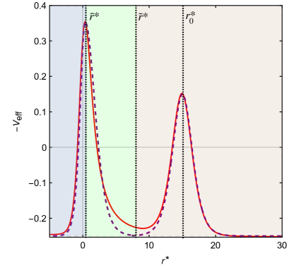
Figure 4: Comparison between the typical effective potential $V_{\text{eff}}$ (red) defined in the text and the generalized Pöschl-Teller potential (purple dashed). We show three regions with different background colors where interface boundary indicates the matching locations.

Now the coefficients $A_{3}$ and $B_{3}$ can be determined from above matching conditions. To read out $A_{H}^{+}$ and $A_{H}^{-}$ for the asymptotical behavior of the solution at $r^{\ast}\rightarrow-\infty$ in (S22) from the solution at $i=3$ in (S26), one more step is to rewrite $h_{3}^{\text{(up)}}$ into a combination of the following plane wave forms by employing the identity of the hypergeometric functions

$${}_{2}F_{1}(a,b;c;y)= \frac{\Gamma(c)\Gamma(c-a-b)}{\Gamma(c-a)\Gamma(c-b)}$$

$$\times_{2}F_{1}(a,b;a+b+1-c;1-y)$$

$$+\frac{\Gamma(c)\Gamma(a+b-c)}{\Gamma(a)\Gamma(b)}(1-y)^{c-a-b}$$

$$\times_{2}F_{1}(c-a,c-b;1+c-a-b;1-y),$$ (S32)

and the relation between associated Legendre polynomial function and hypergeometry function, given by

$$P_{\beta}^{\mu}(y)= \frac{1}{\Gamma(1-\mu)}\left(\frac{1+y}{1-y}\right)^{\mu/2}$$

$$\times_{2}F_{1}\left(-\beta,\beta+1;1-\mu;\frac{1-y}{2}\right),$$ (S33)

where $h_{3}^{(\text{up})}$ can be rewritten asymptotically as

$$h_{3}^{\text{(}up)}(r^{\ast}\rightarrow-\infty)={N}e^{-\mu_{3}r^{\ast}/s_{3}}+{M}e^{\mu_{3}r^{\ast}/s_{3}}$$ (S34)

with

$${N}=\frac{\Gamma(1-\mu_{3})\Gamma(\mu_{3})}{\Gamma(-\beta_{3})\Gamma(1+\beta_{3})},$$

$${M}=\frac{\Gamma(1-\mu_{3})\Gamma(-\mu_{3})}{\Gamma(1-\mu_{3}+\beta_{3})\Gamma(-\mu_{3}-\beta_{3})}.$$ (S35)

One can immediately read off

$$A_{H}^{-}={A}_{3}+{N}{B}_{3},$$ (S36)

$$A_{H}^{+}={M}+{B}_{3}.$$ (S37)

When the mass shell is absent, $A_{3}$ and $B_{3}$ are found in the matching conditions with ${A}_{2}=0$, ${B}_{2}=1$. The spectrum then can be found by $A_{H}^{+}/A_{H}^{-}=0$ [44, 45]. Alternatively, one can start from the $i=3$ region and use (S19) to determine $A_{3}=1$ and $B_{3}=0$. The matching points are still at $\bar{r}^{\ast}$ and $\tilde{r}^{\ast}$. Using the above identity rewrites $h_{1}^{\text{(}in)}$ at $r^{\ast}\rightarrow\infty$. Then $A^{(+)}_{\infty}$ and $A^{(-)}_{\infty}$ can be read off from (S19). The requirement of $A^{(-)}_{\infty}/A^{(+)}_{\infty}=0$ gives the eigenfequency.

Figure 5: The frequencies of the quasinormal mode of the fundamental tone for various uniform Rabi coupling strengths, and $m=1,2,3$.

With reference to [42], we introduce another method suited for a constant mass term. Defining $x=r^{-1}$, we look for a solution

$$H(x)=e^{i\tilde{{\omega}}x^{-1}}\left(\frac{1-x}{1+x}\right)^{-i\left(\omega-m\ell\right)/2}\sum_{k=0}^{\infty}a_{k}\left(1-x\right)^{k},$$ (S38)

where $\tilde{\omega}=\sqrt{\omega^{2}-4\Omega_{0}^{2}}$, $a_{0}=1$ and $\Omega_{0}$ of the Rabi coupling strength is considered as a constant. After substituting it into the Schrodinger-like wave equation in the text, we have four-term recurrence relation given by

$$\alpha_{0}a_{1}+\beta_{0}a_{0}=0,$$ (S39)

$$\alpha_{1}a_{2}+\beta_{1}a_{1}+\gamma_{1}a_{0}=0,$$ (S40)

and

$$\alpha_{k}a_{k+1}+\beta_{k}a_{k}+\gamma_{k}a_{k-1}+\delta_{k}a_{k-2}=0,$$ (S41)

for $k=2,3,\cdots$, where

$$\alpha_{k}= -8\left(1+k\right)\left[(1+k)-i\left(\omega-m\ell\right)\right]\,,$$ (S42)

$$\beta_{k}= 4\big{[}5k^{2}+k\left(5+4im\ell-4i\omega-4i\tilde{\omega}\right)+2m\ell\left(i+\omega+\tilde{\omega}\right),$$

$$+\left(i+m+\omega+\tilde{\omega}\right)\left(-i+m-\omega-\tilde{\omega}\right)\big{]},$$ (S43)

$$\gamma_{k}= -2\left(-3+8k^{2}+4im\ell k-4i\omega k-4i\tilde{\omega}k\right).$$ (S44)

$$\delta_{k}= (1+2k)(-3+2k).$$ (S45)

When the series expansion in (S38) converges to a finite value within $0\leq x\leq 1$, the solution of $H(x)$ satisfies the QNM boundary condition with the asymptotic forms of $e^{i\tilde{\omega}/x}$ at the horizon ($x\rightarrow 1$) and $(1-x)^{-i(\omega-m\ell)/2}e^{i\tilde{\omega}/x}$ at infinity ($x\rightarrow 0$). Furthermore, one can use Gaussian elimination to reduce (S41) to the three-term recurrence relation

$$\alpha_{0}^{\prime}a_{1}+\beta_{0}^{\prime}a_{0}=0,$$ (S46)

$$\alpha_{k}^{\prime}a_{k+1}+\beta_{k}^{\prime}a_{k}+\gamma_{k}^{\prime}a_{k-1}=0,\quad k=1,2,\cdots.$$ (S47)

$\alpha_{k}^{\prime},\,\beta_{k}^{\prime}$ and $\gamma_{k}^{\prime}$ can be expressed in terms of $\alpha_{k},\,\beta_{k},\,\gamma_{k}$, and $\delta_{k}$, given by

$$\alpha_{0}=\alpha_{0}^{\prime},\,\beta_{0}^{\prime}=\beta,\,\gamma_{0}^{\prime}=\gamma_{0}$$ (S48)

$$\alpha_{1}=\alpha_{1}^{\prime},\,\beta_{1}^{\prime}=\beta_{1},\,\gamma_{1}^{\prime}=\gamma_{1}$$ (S49)

$$\alpha_{k}^{\prime}=\alpha_{k},\,\beta_{k}^{\prime}=\beta_{k}-\alpha_{k-1}^{\prime}\delta_{k}/\gamma_{k-1}^{\prime},\quad{and}\quad\gamma_{k}^{\prime}=\gamma_{k}-\beta_{k-1}^{\prime}\delta_{k}/\gamma_{k-1}^{\prime},$$ (S50)

which gives the QNM condition written as

$$\beta_{0}^{\prime}-\frac{\alpha_{0}^{\prime}\gamma_{1}^{\prime}}{\beta_{1}^{\prime}-}\frac{\alpha_{1}^{\prime}\gamma_{2}^{\prime}}{\beta_{2}^{\prime}-}\frac{\alpha_{2}^{\prime}\gamma_{3}^{\prime}}{\beta_{3}^{\prime}-}\cdots=0.$$ (S51)

The complex-frequency roots of the above condition corresponding to a different uniform Rabi coupling strength are shown in Fig. 5. To compare with Fig. 1, the modification of the fundamental mode in a constant $\Omega_{0}$ are not as drastic as in the spatial-dependent one from the case of $\Omega_{0}=0$.

Numerically solving the time-dependent equation in (5) for $H_{m}(r,t)$

In addition to the analysis in frequency domain, we also study the time evolution of the small perturbations in the background of the presence of the spatial dependent mass term. By numerically integrating the equation (5) with the forth-order Runge-Kutta method, we focus on the response of the radial profile $H_{m}(r,t)$ at $r=2$ as a function of time. We consider the initial conditions of the Gaussian pulse

$$H(r^{\ast},t=0)=\exp\left[-(r^{\ast}-\zeta^{\ast})^{2}/2\sigma^{2}\right],$$ (S52)

$$\partial_{t}H(r^{\ast},t=0)=0,$$ (S53)

where $\zeta^{\ast}$ is chosen to be outside the radius of the mass term, and $\sigma$ is the width.

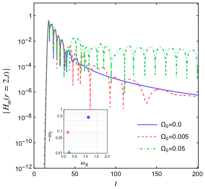
Figure 6: The absolute value of time-domain profile with varying $\Omega_{0}$. The inset figure shows the fundamental QNM frequency with the corresponding value of $\Omega_{0}$. Other parameters are fixed as $m=1$, distance $r_{0}=15,$ and $\alpha=1/2$.

In Fig. 6, we compare three cases with $2\Omega_{0}=0.0$, $0.01$, and $0.1$. Even though the spectrum has significant change for small perturbations, such as $2\Omega_{0}=0.01$, we find that the response waveform in the time domain shows not much difference from the unperturbed one.