Absolute convergence and error thresholds in non-active adaptive sampling

Abstract

Non-active adaptive sampling is a way of building machine learning models from a training data base which are supposed to dynamically and automatically derive guaranteed sample size. In this context and regardless of the strategy used in both scheduling and generating of weak predictors, a proposal for calculating absolute convergence and error thresholds is described. We not only make it possible to establish when the quality of the model no longer increases, but also supplies a proximity condition to estimate in absolute terms how close it is to achieving such a goal, thus supporting decision making for fine-tuning learning parameters in model selection. The technique proves its correctness and completeness with respect to our working hypotheses, in addition to strengthening the robustness of the sampling scheme. Tests meet our expectations and illustrate the proposal in the domain of natural language processing, taking the generation of part-of-speech taggers as case study.

1 Introduction

A recurrent issue in machine learning (ml) relates the determination of optimal sampling data sets, the aim being to reduce both training costs and time without making the modelling process less reliable. In this sense, the operating principle for adaptive sampling is simple and involves beginning with an initial number of examples and then iteratively learning the model, evaluating it and acquiring additional observations if necessary. Accordingly, there are two questions to be considered: it is necessary to determine the training data to be acquired at each cycle, and also to define a halting condition to terminate the loop once a certain degree of performance has been achieved by the learner. Both tasks confer the character of research issues to the formalization of scheduling and stopping criteria (John and Langley, 1996), respectively. The former has been researched for decades in terms of fixed (John and Langley, 1996; Provost et al., 1999) or adaptive (Provost et al., 1999) sequencing, and it is not our objective. As regards the halting criteria, they are independent of the scheduling and mostly start from the hypothesis that learning curves are well-behaved, including an initial steeply sloping portion, a more gently sloping middle one and a final balanced zone (Meek et al., 2002). Accordingly, the purpose is to identify the moment in which such a curve reaches a plateau, namely when adding more data instances does not improve the accuracy, although this often does not strictly verify. Instead, extra learning efforts almost always result in modest increases. This justifies the interest in having a proximity condition, understood as a measure of the degree of convergence attained from a given iteration, rather than a stopping one. In short, this will make it possible to select the level of reliability in predicting a learner’s performance, both in terms of accuracy and computational costs. We will thus have a powerful and flexible decision support tool in the field of model selection, capable of adapting to the user’s needs in terms of the evaluation quality of both the learning strategy and its parameterization.

A major challenge is then to avoid the overvaluation of learning perturbations, in such a way that the training does not stop prematurely due to temporary increases in accuracy. Namely, we are interested in proving the correctness of a proximity criterion with respect to the working hypotheses, but also in improving its capacity to mitigate the impact of such fluctuations without compromising it, i.e. its robustness. Given that we are looking for a practical formula, it is finally necessary to ensure its applicability, which relies on proving the completeness of the approach. These properties focus the attention of this work, the structure of which we briefly describe. Firstly, Section 2 examines the methodologies serving as an inspiration to solve the question posed, as well as our contributions. Next, Section 3 reviews the mathematical basis supporting the proposal, whose model we introduce in Section 4. In Section 5, we describe the testing frame for the experiments illustrated in Section 6. Finally, Section 7 presents the final conclusions.

2 The state of the art

Below is a brief review on how correctness, robustness and completeness have been addressed over time in the definition of halting conditions in adaptive sampling, thus allowing to contextualize our contribution in that respect.

2.1 Working on correctness, robustness and completeness

Regarding correctness, most adaptive samplers assume a set of hypotheses guaranteeing concurrence, such as access to independent and identically distributed observations (Schütze et al., 2006; Tomanek and Hahn, 2008). The learning curve is then monotonic and, since it is bounded, training converges on a supremum. At this point, the conditions for halting are addressed from two viewpoints, depending on whether predictive accuracy is the only factor to take into account (Frey and Fischer, 1999) or just another one in an optimization scenario stated in decision theory (Howard, 1966). In this latter context, performance is understood as the search for a proper cost/benefit trade-off and authors resort to statistically based strategies by applying the principle of maximum expected utility (Meek et al., 2002) (meu). This implies taking all effectiveness considerations into account, which depends on the degree of control exercised by the user on the learning process. In its absence, namely using non-active techniques as we do, the final cost is the sum of data acquisition, error and model induction charges (Weiss and Tian, 2008). Nonetheless, at best, heuristics are used to calculate the first two and there is thus no way of guaranteeing the location of a global optimum (Last, 2009), which often results in assuming fixed budgets (Kapoor and Greiner, 2005). Alternatively, procedures exclusively based on accuracy estimates try to identify the plateau of the learning curve in terms of functional convergence. Among the most popular ones are local detection and learning curve estimation (John and Langley, 1996), or linear regression with local sampling (Provost et al., 1999), all of them based on heuristics. Again, we cannot talk here about proximity criteria, only of stopping conditions. More recently, this issue has been corrected (Vilares et al., 2017), although the proposal is still far from our objective because the proximity is expressed in terms of the net contribution of each iteration to the learning process, which provides not absolute but relative estimates.

Turning to robustness, one common idea is to generate different versions (weak predictors) of the partial learning curves by changing the training data distribution repeatedly, and integrating the hypotheses thus obtained. That way, bagging procedures (Breiman, 1996) build the predictors in parallel to combine them by voting (classification) (Leung and Parker, 2003) or averaging (regression) (Leite and Brazdil, 2007). On the contrary, boosting algorithms (Schapire, 1990) do it sequentially, which allows the adapting of such a distribution from the results observed in previous predictors. This gives rise to arcing strategies (Freund and Schapire, 1996), where increasing weight is placed on the more frequently misclassified observations. Since these are the troublesome points, focusing on them may do better than the neutral bagging approach (Bauer and Kohavi, 1999), justifying (García-Pedrajas and De Haro-García, 2014) its popularity. Another well-known method is the $k$-fold cross validation (Clark et al., 2010), where the sample is randomly partitioned into $k$ equal sized subsamples. For each fold, a model is trained on the other $k-1$ ones and tested on it, which gives an advantage to working with small data sets. The performance reported is the average of the values computed. Whatever the format, such as online proposals, all these build on the observations available, a major constraint for making estimations beyond the last one. One simple way to alleviate this problem is by using anchors (Vilares et al., 2017), i.e. extra examples placed at the point of infinity to generate the weak predictor in each cycle. As any one of such curves is the result of a fitting action, the sum total of its residuals, namely the differences between the observed values and the fitted ones, is null. This gives the anchor the chance to neutralize irregularities by choosing an appropriate value.

Finally, completeness of the halting conditions has received no attention before to the best of our knowledge, probably because so far no additional assumptions on the sampling premises were necessary to provide a practical solution.

2.2 Our contribution

It revolves around foundations, reliability and applicability to provide correctness, robustness and completeness in a context for which the ease of use is a priority. The former is established from a set of working hypotheses widely recognized in ml and a previous outcome, whose interest was only formal to date, on learning convergence in adaptive sampling (Vilares et al., 2017). To that end, the adaptation to the premises of the theoretical result must be guaranteed. The solution is based on the concept of anchoring, also proposed by those authors but only as a robustness mechanism, which requires the development of a specific family of such techniques.

We choose the domain of natural language processing (nlp) as case study, and more precisely the modelling of part-of-speech (pos) taggers, the classifiers that mark a word in a text (corpus) as corresponding to a particular pos, based on its definition and context. The reasons are the significant resource and time costs of generating training data, the complexity of the relations to be learned and the fact that pos tagging is prior to any other nlp task, so errors at this stage can lower its performance (Song et al., 2012). That highlights the scale of the challenge, but also justifies its interest and popularity as experimentation field for new ml facilities, particularly around sampling technology (Bloodgood and Vijay-Shanker, 2009; Lewis and Gale, 1994; Reichart et al., 2010; Schmid and Laws, 2008; Vlachos, 2008), which is the case here.

3 The formal framework

We introduce the concepts underlying the proposal, most of them taken from Vilares et al. (2017), denoting the real numbers by $\mathbb{R}$ and the natural ones by $\mathbb{N}$, assuming that $0\not\in\mathbb{N}$. A prior question to clarify, because the generation of ml-based pos taggers serves as an illustration guide, is the accuracy notion usually accepted in that kind of model. We define it as the number of correctly tagged tokens divided by the total ones, expressed as a percentage (van Halteren, 1999) and calculated following some generally admitted usages: all tokens in the testing data set are counted, including punctuation marks, and it is supposed that only one tag per token is provided.

3.1 The working hypotheses

We start with a sequence of observations calculated from cases incrementally taken from a training data base, meeting some conditions to ensure a predictable progression of the estimates over a virtually infinite interval. So, they are assumed to be independently and identically distributed (Domingo et al., 2002; Schütze et al., 2006; Tomanek and Hahn, 2008). We then accept that a learning curve is a positive definite and strictly increasing function on $\mathbb{N}$, where numbers are the position of the case in the training data base, and upper bounded by 100. This results (Apostol, 2000) in a concave graph with horizontal asymptote. Such hypotheses make up an idealized working frame to support correctness, while real learners may deviate from it, thus justifying the study of robustness. These deviations impact both the concavity and increase of those curves, as shown in the left-most diagram of Fig. 1 for the fast transformation-based learning (fntbl) tagger (Ngai and Florian, 2001) on the Freiburg-Brown (frown) corpus of American English (Mair and Leech, 2007).

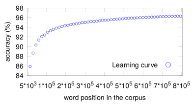
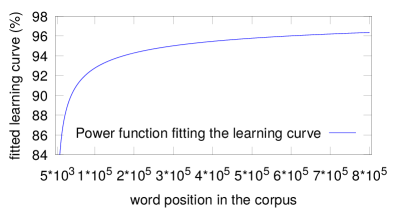
Figure 1: Learning curve for fntbl on frown corpus, and an accuracy pattern fitting it.

3.2 The notational support

Having identified the context of the problem, it is necessary to formalize the data structures we are going to work with, such as the collection of instances whose convergence is intended to be measured.

Definition 1.

(Learning scheme) Let ${\mathcal{D}}$ be a training data base, $\mathcal{K}\subsetneq\mathcal{D}$ a set of initial items from $\mathcal{D}$, and $\sigma:\mathbb{N}\rightarrow\mathbb{N}$ a function. We define a learning scheme for $\mathcal{D}$ with kernel $\mathcal{K}$ and step $\sigma$, as a triple $\mathcal{D}^{\mathcal{K}}_{\sigma}=[\mathcal{K},\sigma,\{\mathcal{D}_{i}\}_{i\in\mathbb{N}}]$, such that $\{\mathcal{D}_{i}\}_{i\in\mathbb{N}}$ is a cover of $\mathcal{D}$ verifying:

$${\mathcal{D}}_{1}:={\mathcal{K}}\mbox{ and }{\mathcal{D}}_{i}:={\mathcal{D}}_{i-1}\cup{\mathcal{I}}_{i},\;\mathcal{I}_{i}\subset{\mathcal{D}}\setminus{\mathcal{D}}_{i-1},\;\left\|{\mathcal{I}}_{i}\right\|=\sigma(i),\;\forall i\geq 2$$ (1)

with $\left\|{\mathcal{I}}_{i}\right\|$ the cardinality of ${\mathcal{I}}_{i}$. We refer to $\mathcal{D}_{i}$ as the individual of level $i$ for $\mathcal{D}^{\mathcal{K}}_{\sigma}$.

A learning scheme relates a level $i$ with the position $\left\|\mathcal{D}_{i}\right\|$ in the training data base, determining the sequence of observations $\{[x_{i},{\mathcal{A}}_{\boldsymbol{\boldsymbol{\infty}}{}}[{\mathcal{D}}](x_{i})],\;x_{i}:=\left\|\mathcal{D}_{i}\right\|\}_{i\in\mathbb{N}}$, where ${\mathcal{A}}_{\boldsymbol{\boldsymbol{\infty}}{}}[{\mathcal{D}}](x_{i})$ is the accuracy achieved on such an instance by the learner. Thus, a level determines an iteration in the adaptive sampling whose learning curve is ${\mathcal{A}}_{\boldsymbol{\boldsymbol{\infty}}{}}[{\mathcal{D}}]$, whilst ${\mathcal{K}}$ delimits a portion of ${\mathcal{D}}$ we believe to be enough to initiate consistent evaluations of the training. For its part, $\sigma$ identifies the sampling scheduling. As we want stable estimates, partial learning curves are extrapolated according to a functional pattern that verifies the working hypotheses, but are also infinitely differentiable. This supplies graphs without disruptions due to instantaneous jumps while ensuring their regularity.

Definition 2.

(Accuracy pattern) Let $C^{\infty}_{(0,\infty)}$ be the C-infinity functions in $\mathbb{R}^{+}$, we say that $\pi:\mathbb{R}^{{+}^{n}}\rightarrow C^{\infty}_{(0,\infty)}$ is an accuracy pattern iff $\pi(a_{1},\dots,a_{n})$ is positive definite, upper bounded, concave and strictly increasing.

An example is the power law family of curves $\pi(a,b,c)(x):=-a*x^{-b}+c$, hereafter used as the running one. Its upper bound is the horizontal asymptote value $\lim\limits_{x\rightarrow\infty}\pi(a,b,c)(x)=c$, and

$$\pi(a,b,c)^{\prime}(x)=a*b*x^{-(b+1)}>0\hskip 21.33955pt\pi(a,b,c)^{\prime\prime}(x)=-a*b*(b+1)*x^{-(b+2)}<0$$ (2)

which guarantees increase and concavity in $\mathbb{R}^{+}$, respectively. This is illustrated in the right-most diagram of Fig. 1, whose goal is to fit the learning curve represented on the left-hand side. Here, the values $a=542.5451$, $b=0.3838$ and $c=99.2876$ are provided by the trust region method (Branch et al., 1999), a regression technique minimizing the summed square of residuals, namely the differences between the observed values and the fitted ones. Furthermore, as the aim is to determine the degree of convergence attained by the learning process, we need to evaluate the progression of accuracy through the sequence of weak predictors being computed.

Definition 3.

(Learning trend) Let $\mathcal{D}^{\mathcal{K}}_{\sigma}$ be a learning scheme, $\pi$ an accuracy pattern and $\ell\in\mathbb{N},\;\ell\geq 3$ a position in the training data base $\mathcal{D}$. We define the learning trend of level $\ell$ for ${\mathcal{D}}^{\mathcal{K}}_{\sigma}$ using $\pi$, as a curve ${\mathcal{A}}_{\ell}^{\pi}[{\mathcal{D}}^{\mathcal{K}}_{\sigma}]\in\pi$, fitting the observations $\{[x_{i},{\mathcal{A}}_{\boldsymbol{\boldsymbol{\infty}}{}}[{\mathcal{D}}](x_{i})],\;x_{i}:=\left\|\mathcal{D}_{i}\right\|\}_{i=1}^{\ell}$. A sequence of learning trends ${\mathcal{A}}^{\pi}[{\mathcal{D}}^{\mathcal{K}}_{\sigma}]:=\{{\mathcal{A}}_{\ell}^{\pi}[{\mathcal{D}}^{\mathcal{K}}_{\sigma}]\}_{\ell\in\mathbb{N}}$ is called a learning trace. We refer to $\{\alpha_{\ell}\}_{\ell\in\mathbb{N}}$ as the asymptotic backbone of ${\mathcal{A}}^{\pi}[{\mathcal{D}}^{\mathcal{K}}_{\sigma}]$, where $y=\alpha_{\ell}:=\lim\limits_{x\rightarrow\infty}{\mathcal{A}}_{\ell}^{\pi}[{\mathcal{D}}^{\mathcal{K}}_{\sigma}](x)$ is the asymptote of ${\mathcal{A}}_{\ell}^{\pi}[{\mathcal{D}}^{\mathcal{K}}_{\sigma}]$.

A learning trend ${\mathcal{A}}_{\ell}^{\pi}[{\mathcal{D}}^{\mathcal{K}}_{\sigma}]$ requires a level $\ell\geq 3$, because we need at least three observations to generate a curve. Its value ${\mathcal{A}}_{\ell}^{\pi}[{\mathcal{D}}^{\mathcal{K}}_{\sigma}](x_{i})$ represents the prediction for accuracy on a case $x_{i}$, using a model generated from the first $\ell$ cycles of the learner. Accordingly, the asymptotic term $\alpha_{\ell}$ is nothing other than the estimate for the highest accuracy attainable. This way, a learning trace gives a comprehensive picture of the increase in accuracy due to new observations, as well as future expectations. Continuing with the tagger fntbl and the corpus frown, Fig. 2 illustrates a portion of the learning trace with kernel and uniform step function $5*10^{3}$, including a zoom view.

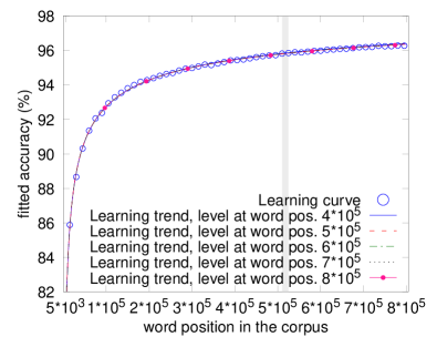
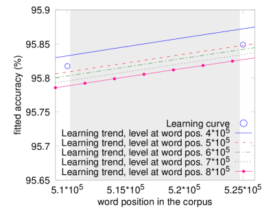
Figure 2: Learning trace for fntbl on frown, with details in zoom.

4 The abstract model

Learning traces lay the foundations for estimating absolute convergence and error thresholds in adaptive sampling (Vilares et al., 2017), thus giving coverage to the correctness we are looking for, while only a relative solution is described in practice. In short, assessing is done from the gain of accuracy between consecutive iterations, which is not enough for our purposes. To overcome this limit, we turn to the concept of anchoring, originally introduced to improve robustness, but which is now also useful to ensure completeness. The problem formulates in terms of the uniform approximation of a learning curve ${\mathcal{A}}_{\boldsymbol{\boldsymbol{\infty}}{}}[{\mathcal{D}}]$ by means of the limit function ${\mathcal{A}}_{\infty}^{\pi}[{\mathcal{D}}^{\mathcal{K}}_{\sigma}]$ for a learning trace ${\mathcal{A}}^{\pi}[{\mathcal{D}}^{\mathcal{K}}_{\sigma}]:=\{{\mathcal{A}}_{i}^{\pi}[{\mathcal{D}}^{\mathcal{K}}_{\sigma}]\}_{i\in\mathbb{N}}$ incrementally built from sampling. We start with a brief reminder of the key results on robustness and correctness. The reader can focus on the less formal aspects, to later address in detail completeness as main contribution.

4.1 Robustness

Real learning conditions may diverge slightly from the ideal ones in the working hypotheses on which correctness is stated. In this sense, robustness is studied in the context of a more flexible set of testing hypotheses. These capture the notion of irregular observation by assuming that learning curves are positive definite and upper bounded by 100, but only quasi-strictly increasing and concave. We then differentiate the alterations according to their position in relation to the working level (wlevel), i.e. the cycle from which they would have a small enough impact to work on their softening. As this depends on unpredictable factors such as the magnitude, distribution and the very existence of these disorders, a heuristic is necessary to identify it. Considering that the model stabilizes as the training advances and that the monotony of the asymptotic backbone is at the basis of the correctness for any halting condition, a way of doing it is to categorize the variations induced in the latter. This allows to estimate wlevel as the level providing the first fluctuation below a given ceiling and, once passed, the prediction level (plevel) marking the beginning for learning trends which could feasibly predict the learning curve, namely not exceeding its maximum (100).

Definition 4.

(Working and prediction levels) Let ${\mathcal{A}}^{\pi}[{\mathcal{D}}^{\mathcal{K}}_{\sigma}]$ be a learning trace with asymptotic backbone $\{\alpha_{i}\}_{i\in\mathbb{N}}$, $\nu\in(0,1)$, $\varsigma\in\mathbb{N}$ and $\lambda\in\mathbb{N}\cup\{0\}$. The working level (wlevel) for ${\mathcal{A}}^{\pi}[{\mathcal{D}}^{\mathcal{K}}_{\sigma}]$ with verticality threshold $\nu$, slowdown $\varsigma$ and look-ahead $\lambda$, is the smallest $\omega(\nu,\varsigma,\lambda)\in\mathbb{N}$ verifying

$$\frac{\sqrt[\varsigma]{\nu}}{1-\nu}\geq\frac{\mid\alpha_{i+1}-\alpha_{i}\mid}{x_{i+1}-x_{i}},\;x_{i}:=\left\|{\mathcal{D}}_{i}\right\|,\;\forall i\mbox{ such that }\omega(\nu,\varsigma,\lambda)\leq i\leq\omega(\nu,\varsigma,\lambda)+\lambda$$ (3)

while the smallest $\wp(\nu,\varsigma,\lambda)\geq\omega(\nu,\varsigma,\lambda)$ with $\alpha_{\wp(\nu,\varsigma,\lambda)}\leq 100$ is the prediction level (plevel). Unless they are necessary for understanding, we shall omit the parameters, referring to wlevel by $\omega$ (resp. plevel by $\wp$).

The wlevel is the first level for which the normalized absolute value of the slope of the line joining consecutive points on the asymptotic backbone is less than the verticality threshold $\nu$, which is corrected by a factor $1/\varsigma$ in order to slow down the normalization pace for $\nu$. In effect, since the absolute value for a slope is defined in the interval $[0,\infty)$, the normalizing function to be applied can be expressed as follows:

$$\begin{array}[]{lccc}\mbox{\sc n}:&[0,\infty)&\longrightarrow&[0,1)\\ &x&\leadsto&\frac{x}{x-1}\end{array}$$ (4)

That way, given two consecutive points $(x_{i},\alpha_{i})$ and $(x_{i+1},\alpha_{i+1})$ in the asymptotic backbone, the absolute slope to be considered and the original condition we are looking for are then, respectively:

$$\frac{\mid\alpha_{i+1}-\alpha_{i}\mid}{x_{i+1}-x_{i}}\hskip 56.9055pt\mbox{and}\hskip 56.9055pt\mbox{\sc n}(\frac{\mid\alpha_{i+1}-\alpha_{i}\mid}{x_{i+1}-x_{i}})<\nu$$ (5)

The latter condition can be easily transformed into the following equivalent one:

$$\frac{\nu}{1-\nu}\geq\frac{\mid\alpha_{i+1}-\alpha_{i}\mid}{x_{i+1}-x_{i}}$$ (6)

from which, including the slowdown factor $1/\varsigma$ and the condition on the look-ahead $\lambda$, we derive Eq. 3. The use of normalized slopes corrected by the slowdown parameter $\varsigma$ allows recursion to infinitely large values and to extremely small decimal fractions to be avoided, thus facilitating the setting of the threshold $\nu$.

Intuitively, since slope values decrease together with the deviations in the monotony studied, we can use them to categorize the latter, taking the look-ahead $\lambda$ as verification window. We then place plevel on the first cycle with a learning trend below 100, which would therefore be the first level with real predictive capacity, since the previous ones would exceed this maximum accuracy value for any model generated. In our example, Fig. 3 shows the scale of such deviations before and after wlevel, for $\nu=2*10^{-5}$, $\varsigma=1$ and $\lambda=5$. Now the way is clear to introduce anchoring as a mechanism for robustness in sampling.

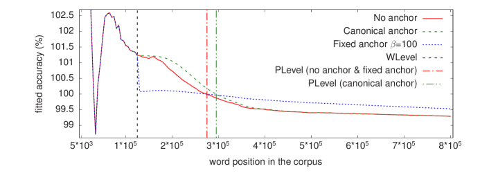
Figure 3: Working and prediction levels without and with canonical anchors for fntbl on frown, with details in zoom.

Definition 5.

(Anchoring learning trace) Let ${\mathcal{A}}^{\pi}[{\mathcal{D}}^{\mathcal{K}}_{\sigma}]$ be a learning trace with wlevel $\omega$, and $\{\hat{\mathcal{A}}_{\ell}(\infty)\}_{\ell>\omega}\subset\mathbb{R}^{+}$. A learning trend of level $\ell>\omega$ with anchor $\hat{\mathcal{A}}_{\ell}(\infty)$ for ${\mathcal{A}}_{\boldsymbol{\boldsymbol{\infty}}{}}[{\mathcal{D}}]$ using the accuracy pattern $\pi$, is a curve $\hat{\mathcal{A}}_{\ell}^{\pi}[{\mathcal{D}}^{\mathcal{K}}_{\sigma}]\in\pi$ fitting the observations $\{[x_{i},{\mathcal{A}}_{\boldsymbol{\boldsymbol{\infty}}{}}[{\mathcal{D}}](x_{i})],\;x_{i}:=\left\|\mathcal{D}_{i}\right\|\}_{i=1}^{\ell}\cup\;[\infty,\hat{\mathcal{A}}_{\ell}(\infty)]$. We denote by $\hat{\rho}_{\ell}(i):=[{\mathcal{A}}_{\boldsymbol{\boldsymbol{\infty}}{}}[{\mathcal{D}}]-\hat{\mathcal{A}}_{\ell}^{\pi}[{\mathcal{D}}^{\mathcal{K}}_{\sigma}]](x_{i})$ the residual of $\hat{\mathcal{A}}_{\ell}^{\pi}[{\mathcal{D}}^{\mathcal{K}}_{\sigma}]$ at the level $i$, by $\hat{\rho}_{\ell}(\infty):=\hat{\mathcal{A}}_{\ell}(\infty)-\hat{\alpha}_{\ell}$ its residual at the point of infinity and by $y=\hat{\alpha}_{\ell}$ its asymptote. When $\{\hat{\alpha}_{\ell}\}_{\ell>\omega}$ is positive definite and converges monotonically to the asymptotic value $\alpha_{\boldsymbol{\boldsymbol{\infty}}{}}$ of ${\mathcal{A}}_{\boldsymbol{\boldsymbol{\infty}}{}}[{\mathcal{D}}]$, we say that $\hat{\mathcal{A}}^{\pi}[{\mathcal{D}}^{\mathcal{K}}_{\sigma}]:=\{\hat{\mathcal{A}}_{\ell}^{\pi}[{\mathcal{D}}^{\mathcal{K}}_{\sigma}]\}_{\ell>\omega}$ is an anchoring learning trace of reference $[{\mathcal{A}}^{\pi}[{\mathcal{D}}^{\mathcal{K}}_{\sigma}],\omega]$.

These new learning trends differ from standard ones in the use of fitting points at infinity, while in practice they are located as far as the computer allows. The use of anchors to improve robustness responds to the idea that extra observations facilitate the realignment of the monotony for the asymptotic backbone, its residual at the point of infinity being the maximum degree of smoothing applicable at a given learning trend. This should be enough for small irregularities, thus limiting the strategy to levels after wlevel. A simple example is canonical anchoring.

Theorem 1.

(Canonical anchoring) Let ${\mathcal{A}}^{\pi}[{\mathcal{D}}^{\mathcal{K}}_{\sigma}]$ be a learning trace with asymptotic backbone $\{\alpha_{i}\}_{i\in\mathbb{N}}$ and $\{\hat{\mathcal{A}}_{i}(\infty)\}_{i>\omega}$ the sequence defined from its wlevel $\omega$ as

$$\hat{\mathcal{A}}_{\omega+1}(\infty):=\alpha_{\omega}\hskip 28.45274pt\hat{\mathcal{A}}_{i+1}(\infty):=\hat{\alpha}_{i}:=\lim\limits_{x\rightarrow\infty}\hat{\mathcal{A}}_{i}^{\pi}[{\mathcal{D}}^{\mathcal{K}}_{\sigma}](x)$$ (7)

with $\hat{\mathcal{A}}_{i}^{\pi}[{\mathcal{D}}^{\mathcal{K}}_{\sigma}]$ a curve fitting $\{[x_{j},{\mathcal{A}}_{\boldsymbol{\boldsymbol{\infty}}{}}[{\mathcal{D}}](x_{j})],\;x_{j}:=\left\|\mathcal{D}_{j}\right\|\}_{j=1}^{i}\cup\;[\infty,\hat{\mathcal{A}}_{i}(\infty)]$, $\forall i>\omega$. Then $\alpha_{\omega+i}\leq\hat{\alpha}_{\omega+i}$ (resp. $\alpha_{\omega+i}\geq\hat{\alpha}_{\omega+i}$), $\forall i\in\mathbb{N}$, when $\{\alpha_{i}\}_{i\in\mathbb{N}}$ is decreasing (resp. increasing). Also, $\{\hat{\mathcal{A}}_{i}^{\pi}[{\mathcal{D}}^{\mathcal{K}}_{\sigma}]\}_{i>\omega}$ is an anchoring learning trace of reference $[{\mathcal{A}}^{\pi}[{\mathcal{D}}^{\mathcal{K}}_{\sigma}],\omega]$, with $\{\hat{\mathcal{A}}_{i}(\infty)\}_{i>\omega}$ its canonical anchors.

Proof 1.

To see in (Vilares et al., 2017). $\blacksquare$

Since in each cycle the anchor takes the value from the asymptote of the last learning trend, the technique described has a conservative nature, which translates into a slower convergence process. The effect of canonical anchoring in smoothing irregularities after the wlevel is illustrated vs. its absence, in our running example by a dashed line, in Fig. 3.

4.2 Correctness

It is addressed from the working hypotheses. That way, the uniform convergence of learning traces has been demonstrated, and the topology of the limit function described.

Theorem 2.

Let ${\mathcal{A}}^{\pi}[{\mathcal{D}}^{\mathcal{K}}_{\sigma}]$ be a learning trace with or without anchors. Then, its asymptotic backbone is monotonic and ${\mathcal{A}}_{\infty}^{\pi}[{\mathcal{D}}^{\mathcal{K}}_{\sigma}]:={\lim\limits_{i\rightarrow\infty}}^{u}{\mathcal{A}}_{i}^{\pi}[{\mathcal{D}}^{\mathcal{K}}_{\sigma}]$ exists, is positive definite, increasing, continuous and upper bounded by 100 in $(0,\infty)$.

Proof 2.

To see in (Vilares et al., 2017). $\blacksquare$

This provides a way to estimate a learning curve ${\mathcal{A}}_{\boldsymbol{\boldsymbol{\infty}}{}}[{\mathcal{D}}]$ by iteratively approximating the function ${\mathcal{A}}_{\infty}^{\pi}[{\mathcal{D}}^{\mathcal{K}}_{\sigma}]$, while a proximity criterion also needs to measure the convergence (resp. error) threshold at each stage. Namely, after fixing a level $i$ in a learning trace ${\mathcal{A}}^{\pi}[{\mathcal{D}}^{\mathcal{K}}_{\sigma}]$, we have to calculate an upper bound for the distance between ${\mathcal{A}}_{j}^{\pi}[{\mathcal{D}}^{\mathcal{K}}_{\sigma}]$ and ${\mathcal{A}}_{\infty}^{\pi}[{\mathcal{D}}^{\mathcal{K}}_{\sigma}]$ (resp. ${\mathcal{A}}_{\boldsymbol{\boldsymbol{\infty}}{}}[{\mathcal{D}}]$) in the interval $[\left\|{\mathcal{D}}_{j}\right\|,\infty),\;\forall j\geq i$.

A previous result is needed. Let $\{(q_{i,x}^{i-1},q_{i,y}^{i-1})\}_{i\geq 4}$ (resp. $\{(p_{i,x}^{i-1},p_{i,y}^{i-1})\}_{i\geq 4}$) be the sequence of the last (resp. first, if existing) points in ${\mathcal{A}}_{i}^{\pi}[{\mathcal{D}}^{\mathcal{K}}_{\sigma}]\cap{\mathcal{A}}_{i-1}^{\pi}[{\mathcal{D}}^{\mathcal{K}}_{\sigma}]$. Then, $\{q_{i,x}^{i-1}\}_{i\geq 4}$ and $\{q_{i,y}^{i-1}\}_{i\geq 4}$ (resp. $\{p_{i,x}^{i-1}\}_{i\geq 4}$ and $\{p_{i,y}^{i-1}\}_{i\geq 4}$) are monotonic, except perhaps when there is a transition from one (resp. two) to two (resp. one) intersection points at a level $\imath$, or when we introduce/modify anchors. In that case, $q_{\imath,y}^{\imath-1}$ and $q_{\imath+1,y}^{\imath}$ (resp. $p_{\imath,y}^{\imath-1}$ and $p_{\imath+1,y}^{\imath}$) may momentarily invert their relative positions, and the same applies to $q_{\imath,x}^{\imath-1}$ and $q_{\imath+1,x}^{\imath}$ (resp. $p_{\imath,x}^{\imath-1}$ and $p_{\imath+1,x}^{\imath}$). We then say that $\imath$ is a level of rupture for ${\mathcal{A}}^{\pi}[{\mathcal{D}}^{\mathcal{K}}_{\sigma}]$. The order in $\mathbb{N}$ is also extended to $\boldsymbol{\mathbb{N}}:=\mathbb{N}\cup\{\infty,\boldsymbol{\boldsymbol{\infty}}{}\}$, in such a way that $\boldsymbol{\boldsymbol{\infty}}{}>\infty>i>0,\;\forall i\in\mathbb{N}$.

Theorem 3.

(Correctness) Let ${\mathcal{A}}^{\pi}[{\mathcal{D}}^{\mathcal{K}}_{\sigma}]$ be a learning trace with or without anchors, with wlevel $\omega$, and $y=\alpha_{i}$ the asymptote for ${\mathcal{A}}_{i}^{\pi}[{\mathcal{D}}^{\mathcal{K}}_{\sigma}],\;\forall i\in\boldsymbol{\mathbb{N}}:=\mathbb{N}\cup\{\infty,\boldsymbol{\boldsymbol{\infty}}{}\}$. Let also $(q_{i,x}^{i-1},q_{i,y}^{i-1})$ be the last point in ${\mathcal{A}}_{i}^{\pi}[{\mathcal{D}}^{\mathcal{K}}_{\sigma}]\cap{\mathcal{A}}_{i-1}^{\pi}[{\mathcal{D}}^{\mathcal{K}}_{\sigma}],\;\forall i\geq 4,\;i\neq\imath$, with $\imath$ level of rupture for ${\mathcal{A}}^{\pi}[{\mathcal{D}}^{\mathcal{K}}_{\sigma}]$. We then have, using for the occasion the notation ${\mathcal{A}}_{\boldsymbol{\boldsymbol{\infty}}{}}^{\pi}[{\mathcal{D}}^{\mathcal{K}}_{\sigma}]$ to refer ${\mathcal{A}}_{\boldsymbol{\boldsymbol{\infty}}{}}[{\mathcal{D}}]$, that

$$\mid[{\mathcal{A}}_{k}^{\pi}-{\mathcal{A}}_{j}^{\pi}][{\mathcal{D}}^{\mathcal{K}}_{\sigma}](x)\mid\leq\varepsilon_{i}:=\mid q_{i,y}^{i-1}-\alpha_{i}\mid,\;\forall k,j\geq i\geq 4,\;\forall x\in[q_{i,x}^{i-1},\infty)$$ (8)

$$\mbox{\em(resp. }\mid[{\mathcal{A}}_{k}^{\pi}-{\mathcal{A}}_{j}^{\pi}][{\mathcal{D}}^{\mathcal{K}}_{\sigma}](x)\mid\leq\varepsilon_{i}:=\mid q_{\boldsymbol{\boldsymbol{\infty}}{},y}^{i}-\alpha_{\boldsymbol{\boldsymbol{\infty}}{}}\mid,\;\forall k,j\geq i\geq 1,\;\forall x\in[q_{\boldsymbol{\boldsymbol{\infty}}{},x}^{i},\infty)\mbox{\em)}$$ (9)

if $\{\alpha_{i}\}_{i>\omega+1}$ is decreasing (resp. increasing), with $\{\varepsilon_{i}\}_{i>\omega+1}$ decreasing and convergent to $0$

Proof 3.

To see in (Vilares et al., 2017). $\blacksquare$

This result establishes the uniform convergence (Apostol, 2000) of the learning trace ${\mathcal{A}}^{\pi}[{\mathcal{D}}^{\mathcal{K}}_{\sigma}]$ to the learning curve ${\mathcal{A}}_{\boldsymbol{\boldsymbol{\infty}}{}}[{\mathcal{D}}_{\sigma}]$. In particular, this implies that the curve ${\mathcal{A}}_{\infty{}}^{\pi}[{\mathcal{D}}^{\mathcal{K}}_{\sigma}]$ we are iteratively approximating matches the latter if the training process is long enough and, therefore, $\alpha_{\infty}=\alpha_{\boldsymbol{\boldsymbol{\infty}}}$. Sadly, the result only has a practical reading when the asymptotic backbone is decreasing, as it was in Fig. 2. Otherwise, the bound depends on the final accuracy we want to estimate ($\alpha_{\boldsymbol{\boldsymbol{\infty}}{}}$), as with opennlp maxent (see opennlp.apache.org/) on the section of the Wall Street Journal (wsj) in the penn treebank (Marcus et al., 1999). In this case, the asymptotic backbone is increasing, as reflects the continuous line in Fig. 4. This gap must therefore be closed to guarantee the operability of the approach.

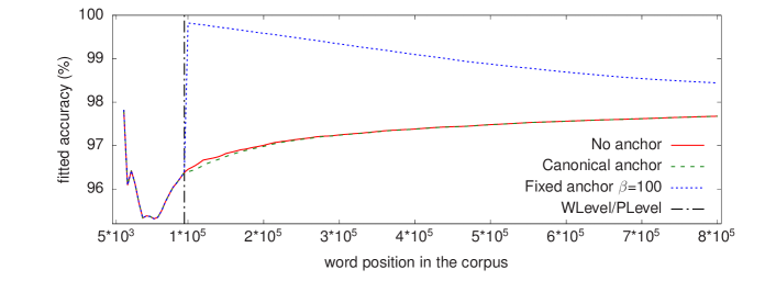
Figure 4: Asymptotic backbones without and with fixed anchors for maxent on penn.

4.3 Completeness

The bulk of our work focuses on this issue, through research on anchoring as a tool to force the dynamics of convergence on learning traces and obtain a decreasing asymptotic backbone, thus ensuring the completeness sought. As a first step, we introduce a sufficient condition to identify anchors verifying such a property.

Theorem 4.

Let ${\mathcal{A}}^{\pi}[{\mathcal{D}}^{\mathcal{K}}_{\sigma}]$ be a learning trace with wlevel $\omega$ and plevel $\wp$, $y=\alpha_{\boldsymbol{\boldsymbol{\infty}}{}}$ the asymptote for the learning curve ${\mathcal{A}}_{\boldsymbol{\boldsymbol{\infty}}{}}[{\mathcal{D}}]$ and $\{\hat{\mathcal{A}}_{i}(\infty)\}_{i>\omega}\subset\mathbb{R}^{+}$ a convergent sequence such that:

$$\hat{\mathcal{A}}_{i}(\infty)\geq\alpha_{i},\;\forall i>\wp$$ (10)

$$\hat{\mathcal{A}}_{i}(\infty)-\hat{\mathcal{A}}_{i+1}(\infty)\geq\hat{\rho}_{i}(\infty)-\hat{\rho}_{i+1}(\infty),\;\forall i>\omega$$ (11)

Let also $\hat{\mathcal{A}}_{i}^{\pi}[{\mathcal{D}}^{\mathcal{K}}_{\sigma}]$ be the learning trend with anchor $\hat{\mathcal{A}}_{i}(\infty)$ and asymptote $y=\hat{\alpha}_{i}$, and $\hat{\rho}_{i}(\infty):=\hat{\mathcal{A}}_{i}(\infty)-\hat{\alpha}_{i},\;\forall i>\omega$. Then, $\{\hat{\mathcal{A}}_{i}^{\pi}[{\mathcal{D}}^{\mathcal{K}}_{\sigma}]\}_{i>\omega}$ is an anchoring learning trace of reference $[{\mathcal{A}}^{\pi}[{\mathcal{D}}^{\mathcal{K}}_{\sigma}],\omega]$, such that $\{\hat{\alpha}_{i}\}_{i>\omega}$ is decreasing.

Proof 4.

To see in Appendix A. $\blacksquare$

So, a criterion to generate a learning trace with decreasing backbone is to select a set of anchors never below the accuracy extrapolated at each cycle to the total training data base (10), as long as the learner does not override the readjustment applied by the anchoring (11). Intuitively simple, we will first study the practical utility of this idea for the case of the previously introduced canonical anchors.

Theorem 5.

Let $\hat{\mathcal{A}}^{\pi}[{\mathcal{D}}^{\mathcal{K}}_{\sigma}]$ be a learning trace with canonical anchoring. We then have that if the asymptotic backbone of the reference is decreasing, then the same thing applies to that of the former.

Proof 5.

To see in Appendix A. $\blacksquare$

Unfortunately, this result does not settle the question at hand, i.e. to guarantee decreasing asymptotic backbones by using anchors in order to have a practical absolute measure of the convergence of learning traces. As shown above, when using a canonical approach, this is ensured only if the reference already verifies it. Otherwise, the resulting asymptotic backbone can also be increasing, as is shown by the dashed line in Fig. 4, and another anchoring strategy is needed to respond to the challenge.

4.3.1 Fixed anchoring

Learning trends are fitting curves on the set of observations available at that time and, when using anchoring, also the value of the latter associated to the point of infinity. This is the key to making the proximity criterion in Theorem 3 fully operational, because the sum total of residuals on such curves is null. So, to achieve decreasing asymptotic backbones it suffices to fix anchors with negative or null residual, which is to say that they must rise above all existing and future observations, for example using values higher or equal than the maximum accuracy (100).

Theorem 6.

(Fixed anchoring) Let ${\mathcal{A}}^{\pi}[{\mathcal{D}}^{\mathcal{K}}_{\sigma}]$ be a learning trace with wlevel $\omega$ and $\hat{\mathcal{A}}_{i}^{\stackrel{{\scriptstyle\beta}}{{\pi}}}[{\mathcal{D}}^{\mathcal{K}}_{\sigma}]$ the learning trend with anchor $\hat{\mathcal{A}}_{i}^{\beta}(\infty):=\beta\geq 100,\forall i>\omega$. Then, $\hat{\mathcal{A}}^{\stackrel{{\scriptstyle\beta}}{{\pi}}}[{\mathcal{D}}^{\mathcal{K}}_{\sigma}]:=\{\hat{\mathcal{A}}_{i}^{\stackrel{{\scriptstyle\beta}}{{\pi}}}[{\mathcal{D}}^{\mathcal{K}}_{\sigma}]\}_{i>\omega}$ is an anchoring learning trace of reference $[{\mathcal{A}}^{\pi}[{\mathcal{D}}^{\mathcal{K}}_{\sigma}],\omega]$ with asymptotic backbone decreasing. We call $\{\hat{\mathcal{A}}_{i}^{\beta}(\infty)\}_{i>\omega}$ the fixed anchors of value $\beta$ for $\hat{\mathcal{A}}^{\stackrel{{\scriptstyle\beta}}{{\pi}}}[{\mathcal{D}}^{\mathcal{K}}_{\sigma}]$.

Proof 6.

To see in Appendix A. $\blacksquare$

Fixed anchoring therefore guarantees the hypotheses under which we can determine a computable estimation of the convergence and error thresholds in absolute terms. Namely, it allows us to generate learning traces with decreasing asymptotic backbones, regardless of the training process considered. An example of this is shown in Fig. 4, where the monotony of the starting asymptotic backbone changes from increasing to decreasing when using fixed anchors of value $\beta=100$. In these conditions, the completeness of our abstract model derives immediately.

Theorem 7.

(Completeness) Let $\hat{\mathcal{A}}^{\stackrel{{\scriptstyle\beta}}{{\pi}}}[{\mathcal{D}}^{\mathcal{K}}_{\sigma}]$ be a learning trace of fixed anchoring with wlevel $\omega$ and $y=\alpha_{i}$ the asymptote for $\hat{\mathcal{A}}_{i}^{\stackrel{{\scriptstyle\beta}}{{\pi}}}[{\mathcal{D}}^{\mathcal{K}}_{\sigma}],\;\forall i\in\boldsymbol{\mathbb{N}}:=\mathbb{N}\cup\{\infty,\boldsymbol{\boldsymbol{\infty}}{}\}$. Let also be $(q_{i,x}^{i-1},q_{i,y}^{i-1})$ the last point in $\hat{\mathcal{A}}_{i}^{\stackrel{{\scriptstyle\beta}}{{\pi}}}[{\mathcal{D}}^{\mathcal{K}}_{\sigma}]\cap\hat{\mathcal{A}}_{i-1}^{\stackrel{{\scriptstyle\beta}}{{\pi}}}[{\mathcal{D}}^{\mathcal{K}}_{\sigma}],\;\forall i\geq 4,\;i\neq\imath$, with $\imath$ level of rupture for $\hat{\mathcal{A}}^{\stackrel{{\scriptstyle\beta}}{{\pi}}}[{\mathcal{D}}^{\mathcal{K}}_{\sigma}]$. We then have, using for the occasion the notation $\hat{\mathcal{A}}_{\infty{}}^{\stackrel{{\scriptstyle\beta}}{{\pi}}}[{\mathcal{D}}^{\mathcal{K}}_{\sigma}]$ (resp. $\hat{\mathcal{A}}_{\boldsymbol{\boldsymbol{\infty}}{}}^{\stackrel{{\scriptstyle\beta}}{{\pi}}}[{\mathcal{D}}^{\mathcal{K}}_{\sigma}]$) to refer ${\mathcal{A}}_{\infty}^{\pi}[{\mathcal{D}}^{\mathcal{K}}_{\sigma}]$ (resp. ${\mathcal{A}}_{\boldsymbol{\boldsymbol{\infty}}{}}[{\mathcal{D}}]$), that

$$\mid[\hat{\mathcal{A}}_{k}^{\stackrel{{\scriptstyle\beta}}{{\pi}}}-\hat{\mathcal{A}}_{j}^{\stackrel{{\scriptstyle\beta}}{{\pi}}}][{\mathcal{D}}^{\mathcal{K}}_{\sigma}](x)\mid\leq\varepsilon_{i}:=\mid q_{i,y}^{i-1}-\alpha_{i}\mid,\;\forall k,j\geq i>\omega+1,\;\forall x\in[q_{i,x}^{i-1},\infty)$$ (12)

with $\{\varepsilon_{i}\}_{i>\omega+1}$ decreasing and convergent to $0$. We call the smallest $\iota\geq 4$ for which $\mid q_{\iota,y}^{\iota-1}-\alpha_{\iota}\mid\leq\tau$, the threshold level for $\tau\in\mathbb{R}^{+}$.

Proof 7.

To see in Appendix A. $\blacksquare$

Contrary to what happened with canonical anchors, the fixed ones free us from checking the decrease in the asymptotic backbone. Following Theorem 3, this provides a practical and extremely simple criterion for implementing a proximity condition measuring absolute thresholds, henceforward referred to as $\mathcal{H}_{a}$.

More in detail, given a learning trace with fixed anchoring $\hat{\mathcal{A}}^{\stackrel{{\scriptstyle\beta}}{{\pi}}}[{\mathcal{D}}^{\mathcal{K}}_{\sigma}]$ and a value $\tau\in\mathbb{R}^{+}$, we can assure that, once the corresponding threshold level $\iota$ has been located:

$$\mid[\hat{\mathcal{A}}_{\infty}^{\stackrel{{\scriptstyle\beta}}{{\pi}}}-\hat{\mathcal{A}}_{j}^{\stackrel{{\scriptstyle\beta}}{{\pi}}}][{\mathcal{D}}^{\mathcal{K}}_{\sigma}](x)\mid\leq\varepsilon_{\iota}:=\mid q_{\iota,y}^{\iota-1}-\alpha_{\iota}\mid\leq\tau,\;\forall j\geq\iota>\omega+1,\;\forall x\in[q_{\iota,x}^{\iota-1},\infty)$$ (13)

Namely, all estimates in the interval $[q_{\iota,x}^{\iota-1},\infty)\supseteq[\left\|\mathcal{D}_{\iota}\right\|,\infty)$ for the learning trends computed from the $\iota$ level are at a distance from the curve ${\mathcal{A}}_{\infty}^{\pi}[{\mathcal{D}}^{\mathcal{K}}_{\sigma}]$ to which we converge (resp. the learning curve ${\mathcal{A}}_{\boldsymbol{\boldsymbol{\infty}}{}}[{\mathcal{D}}]$), which is less than the threshold $\tau$ set.

As for canonical anchors, the fixed ones also contribute to a litte delay in the convergence, as can be seen in Fig. 3 because their values are always higher than the asymptotes associated with the learning trends. One way to reduce this undesirable side effect is to provide the anchoring with mechanisms that allow it to adapt to the dynamics of the learning process.

4.3.2 Endowing fixed anchoring with flexibility

The goal is to define a configurable family of anchorings ensuring the completeness of the proposal, thus allowing us to control the performance via an appropriate setting. Our starting point is the fixed anchor concept described above. Since the residuals at the point of infinity are then negative, we can fine tune anchors from the approximations for accuracy generated as learning progresses, without compromising our objective.

Theorem 8.

(Fixed anchoring with look-ahead) Let ${\mathcal{A}}^{\pi}[{\mathcal{D}}^{\mathcal{K}}_{\sigma}]$ be a learning trace with plevel $\wp$, $\beta\geq 100$, $\ell\in\mathbb{N}$ and $\{\hat{\mathcal{A}}_{i}^{\beta,\ell}(\infty)\}_{i>\omega}$ the sequence defined from its wlevel $\omega$ by

$$\hat{\mathcal{A}}_{i}^{\beta,\ell}(\infty):=\beta,\;\forall\;\wp+\ell+1>i>\omega\hskip 28.45274pt\hat{\mathcal{A}}_{i}^{\beta,\ell}(\infty):=\hat{\alpha}_{\wp+\ell}^{\beta,\ell},\;\forall i\geq\wp+\ell+1$$ (14)

Let also $\hat{\mathcal{A}}_{i}^{\stackrel{{\scriptstyle\beta,\ell}}{{\pi}}}[{\mathcal{D}}^{\mathcal{K}}_{\sigma}]$ be the learning trend with anchor $\hat{\mathcal{A}}_{i}^{\beta,\ell}(\infty),\forall i>\omega$. Then, $\hat{\mathcal{A}}^{\stackrel{{\scriptstyle\beta,\ell}}{{\pi}}}[{\mathcal{D}}^{\mathcal{K}}_{\sigma}]:=\{\hat{\mathcal{A}}_{i}^{\stackrel{{\scriptstyle\beta,\ell}}{{\pi}}}[{\mathcal{D}}^{\mathcal{K}}_{\sigma}]\}_{i>\omega}$ is an anchoring learning trace of reference $[{\mathcal{A}}^{\pi}[{\mathcal{D}}^{\mathcal{K}}_{\sigma}],\omega]$ and asymptotic backbone $\{\hat{\alpha}_{i}^{\beta,\ell}\}_{i>\omega}$ decreasing, and we call $\{\hat{\mathcal{A}}_{i}^{\beta,\ell}(\infty)\}_{i>\omega}$ its set of fixed anchors with look-ahead $\ell$ and value $\beta$.

Proof 8.

To see in Appendix A. $\blacksquare$

Intuitively, we are talking about a learning trace with conventional fixed anchoring, in which the anchor is subject to revision once the study of the levels in the interval $[\omega+1,\wp+\ell]$ has been completed. Since $\omega\leq\wp$, this interval includes $[\wp+1,\wp+\ell]$, which in either case allows us to take advantage of the knowledge provided by the first $\ell$ iterations from the plevel $\wp$. As these are the best performing training cycles – together with the one associated with level $\wp$, in the case where $\omega=\wp$ – among those with real predictive capability, convergence can be expected to accelerate significantly once the anchor has been updated.

To illustrate this, we look again at the learning process shown in Fig. 4, to compare in Fig. 5 the asymptotic backbones associated to some value/look-ahead combinations, focusing on two use cases: different look-aheads ($\imath=0$ and $\imath=41$) with the same value ($\beta=100$) and the same look-ahead ($\imath=0$) with different values ($\beta=100$ and $\beta=101$). In the former scenario, we check how a non-trivial look-ahead ($\imath=41$) causes the desired effect. Also, as might be expected, the second one suggests that the closer the anchor to the real accuracy, the faster the convergence. All the above underscores the importance of an in-depth study on the impact of values and look-aheads on accuracy prediction. The objective is to establish whether these first impressions have a formal basis that allows us to effectively categorize the anchoring strategies described.

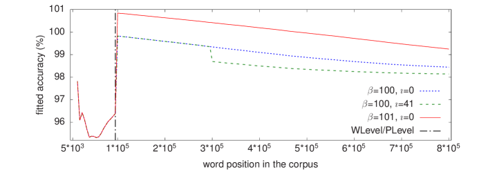
Figure 5: Asymptotic backbones with fixed anchors for maxent on penn (look-ahead $\imath$, value $\beta$).

Theorem 9.

(Anchoring categorization) Let $\hat{\mathcal{A}}^{\pi}[{\mathcal{D}}^{\mathcal{K}}_{\sigma}]$, $\hat{\mathcal{A}}^{\stackrel{{\scriptstyle\eta,\imath}}{{\pi}}}[{\mathcal{D}}^{\mathcal{K}}_{\sigma}]$, $\hat{\mathcal{A}}^{\stackrel{{\scriptstyle\beta,\imath}}{{\pi}}}[{\mathcal{D}}^{\mathcal{K}}_{\sigma}]$ and $\hat{\mathcal{A}}^{\stackrel{{\scriptstyle\beta,\jmath}}{{\pi}}}[{\mathcal{D}}^{\mathcal{K}}_{\sigma}]$ be learning traces of reference $[{\mathcal{A}}^{\pi}[{\mathcal{D}}^{\mathcal{K}}_{\sigma}],\omega]$, generated from canonical and fixed anchors with look-aheads $\imath,\jmath\in\mathbb{N}\cup\{0\}$ for values $\eta,\beta\geq 100$ respectively. We then have that, in any case (resp. when $\{\alpha_{i}\}_{i\in\mathbb{N}}$ decreasing), it verifies that $\forall i>\omega$

$$\mid\alpha_{i}-\alpha_{\boldsymbol{\boldsymbol{\infty}}{}}\mid\leq\mid\hat{\alpha}_{i}-\alpha_{\boldsymbol{\boldsymbol{\infty}}{}}\mid$$ (15)

and also $\forall\jmath>\imath,\eta>\beta,i\geq\wp+\jmath$

$$\mid\hat{\alpha}_{i}^{\beta,\jmath}-\alpha_{\boldsymbol{\boldsymbol{\infty}}{}}\mid\leq\mid\hat{\alpha}_{i}^{\beta,\imath}-\alpha_{\boldsymbol{\boldsymbol{\infty}}{}}\mid\leq\mid\hat{\alpha}_{i}^{\eta,\imath}-\alpha_{\boldsymbol{\boldsymbol{\infty}}{}}\mid$$ (16)

$$(\mbox{resp. }\mid\alpha_{i}-\alpha_{\boldsymbol{\boldsymbol{\infty}}{}}\mid\leq\mid\hat{\alpha}_{i}-\alpha_{\boldsymbol{\boldsymbol{\infty}}{}}\mid\leq\mid\hat{\alpha}_{i}^{\beta,\jmath}-\alpha_{\boldsymbol{\boldsymbol{\infty}}{}}\mid\leq\mid\hat{\alpha}_{i}^{\beta,\imath}-\alpha_{\boldsymbol{\boldsymbol{\infty}}{}}\mid\leq\mid\hat{\alpha}_{i}^{\eta,\imath}-\alpha_{\boldsymbol{\boldsymbol{\infty}}{}}\mid)$$ (17)

with $\{\hat{\alpha}_{i}\}_{i>\omega}$, $\{\hat{\alpha}_{i}^{\eta,\imath}\}_{i>\omega}$, $\{\hat{\alpha}_{i}^{\beta,\imath}\}_{i>\omega}$, $\{\hat{\alpha}_{i}^{\beta,\jmath}\}_{i>\omega}$ and $\{\alpha_{i}\}_{i\in\mathbb{N}}$ their corresponding asymptotic backbones, and $\alpha_{\boldsymbol{\boldsymbol{\infty}}{}}$ the asymptotic value for the learning curve ${\mathcal{A}}_{\boldsymbol{\boldsymbol{\infty}}{}}[{\mathcal{D}}]$.

Proof 9.

To see in Appendix A. $\blacksquare$

The result guides the choice of anchoring. So, the fastest way to converge when the working hypotheses verify is to avoid fixed anchors, except if the asymptotic backbone is not decreasing. When this is quasi-decreasing because only the testing hypotheses are guaranteed, the canonical strategy is the most adequate. Finally, fixed anchoring with look-ahead is the alternative when no data about the training are available. The convergence speed here is inversely proportional to the value, which is why the best option is 100, the minimum one. Once a value is selected, the look-ahead introduces an extra factor to speed up the convergence according to its length, but only from the time the anchor is updated. Because of this, our objective could be reached before the latter is activated, in such a way that a smaller look-ahead might be more effective. Namely, an optimal choice depends on the convergence threshold – that matches, by Theorem 3, the error one – we are trying to identify, thus suggesting an iterative approach for dealing with it. We then make the decision to depend on the degree of convergence reached with respect to that threshold, taking into account that the first reliable level for predictions is plevel.

Definition 6.

(Percentage of uncovered threshold) Let $\hat{\mathcal{A}}^{\stackrel{{\scriptstyle\beta}}{{\pi}}}[{\mathcal{D}}^{\mathcal{K}}_{\sigma}]$ be a learning trace with fixed anchoring and plevel $\wp$, and $\tau$ a threshold for a proximity condition ${\mathcal{H}}$. We define its percentage of uncovered threshold for $\tau$ on ${\mathcal{H}}$ at a level $\ell>\wp+1$ as

$$\mbox{\sc put}[\hat{\mathcal{A}}^{\stackrel{{\scriptstyle\beta}}{{\pi}}}[{\mathcal{D}}^{\mathcal{K}}_{\sigma}],\tau,{\mathcal{H}}](\ell):=\left\{\begin{array}[]{ll}100*\frac{\mid\alpha_{\boldsymbol{\boldsymbol{\infty}}{}}-\hat{\alpha}_{\ell}^{\beta}\mid_{\mathcal{H}}-\tau}{\mid\alpha_{\boldsymbol{\boldsymbol{\infty}}{}}-\hat{\alpha}_{\wp+2}^{\beta}\mid_{\mathcal{H}}-\tau}&\mbox{if}\;\;\mid\alpha_{\boldsymbol{\boldsymbol{\infty}}{}}-\hat{\alpha}_{\ell}^{\beta}\mid_{\mathcal{H}}\geq\tau\\ 0&\mbox{otherwise}\end{array}\right.$$ (18)

with $\mid\alpha_{\boldsymbol{\boldsymbol{\infty}}{}}-\hat{\alpha}_{\ell}^{\beta}\mid_{\mathcal{H}}$ the estimates of ${\mathcal{H}}$ for $\mid\alpha_{\boldsymbol{\boldsymbol{\infty}}{}}-\hat{\alpha}_{\ell}^{\beta}\mid$, and $\hat{\alpha}_{\ell}^{\beta}$ (resp. $\alpha_{\boldsymbol{\boldsymbol{\infty}}{}}$) the asymptotic value for the learning trend (resp. learning curve) $\hat{\mathcal{A}}_{\ell}^{\stackrel{{\scriptstyle\beta}}{{\pi}}}[{\mathcal{D}}^{\mathcal{K}}_{\sigma}]$ (resp. ${\mathcal{A}}_{\boldsymbol{\boldsymbol{\infty}}{}}[{\mathcal{D}}]$).

The put takes values in the interval $[0,100]$ and is decreasing in the level covered. Its geometric interpretation is shown in Fig. 6. Its minimum is 0 and is reached when the estimated degree of approximation improves or equals the threshold $\tau$ set by the user, in asymptotic terms. That is, when the efficiency of the last asymptotic value as fixed anchor can no longer be improved, which implies that the current level is the last one at which a possible update of the fixed anchor based on learning asymptotic values makes sense. As for the maximum value, it is reached at level $\wp+2$, the first at which the anchor could be updated and is $100$, unless at that point the convergence is already effective.

Once we have captured the concept of put and the user has selected a particular value, we can assess for which particular level a fixed anchoring should be updated. That is, we are in a position to determine the look-ahead that matches the user’s requirements.

Definition 7.

(Minimal look-ahead for a tentative put value in fixed anchoring) Let $\hat{\mathcal{A}}^{\stackrel{{\scriptstyle\beta}}{{\pi}}}[{\mathcal{D}}^{\mathcal{K}}_{\sigma}]$ be a learning trace with fixed anchoring and plevel $\wp$, $\tau$ a threshold for a proximity condition ${\mathcal{H}}$ and $\zeta\in[0,100]$ the put value we want to reach before updating the anchor. We then define

$$\lambda:=\min_{\ell>\wp+1}\{\mbox{\sc put}[\hat{\mathcal{A}}^{\stackrel{{\scriptstyle\beta}}{{\pi}}}[{\mathcal{D}}^{\mathcal{K}}_{\sigma},\tau,{\mathcal{H}}](\ell)\leq\zeta\}-\wp$$ (19)

as the minimal look-ahead for the tentative put value $\zeta$.

Formally, the fact that put is monotonic and bound guarantees that the concept of minimal look-ahead is well-defined (Apostol, 2000). Regarding its geometric interpretation and calculation process, both of them are schematized in Fig. 6. We start from the asympotic values $\alpha_{\boldsymbol{\boldsymbol{\infty}}{}}$, $\hat{\alpha}_{\ell}^{\beta}$ and $\hat{\alpha}_{\wp+2}^{\beta}$, which respectivelly correspond to the learning curve, the last learning trend and the first one for which the fixed anchor could be updated. We can then estimate, according the ${\mathcal{H}}$ criterion, the distance yet to be completed from the current level (resp. the first level at which a look-ahead would be applicable) to reach the required convergence threshold, by means of the value $\mid\alpha_{\boldsymbol{\boldsymbol{\infty}}{}}-\hat{\alpha}_{\ell}^{\beta}\mid_{\mathcal{H}}-\tau$ (resp. $\mid\alpha_{\boldsymbol{\boldsymbol{\infty}}{}}-\hat{\alpha}_{\wp+2}^{\beta}\mid_{\mathcal{H}}-\tau$).

By way of illustration, assuming that we want the update of a fixed anchoring to be activated once half of the convergence distance has been covered, it is sufficient to identify the first level $\ell>\wp+1$ at which the put is less than or equal to $50$ and then choose $\lambda:=\ell-\wp$ as the minimal look-ahead for that tentative value. Returning to the example in Fig. 5 when the value of the fixed anchoring for the learning trace is $\beta=100$, this results in a look-ahead of $41$, whose associated asymptotic backbone shows the best results from among those represented.

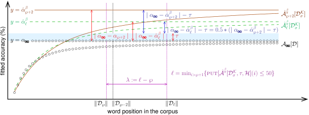
Figure 6: Computing the minimal look-ahead $\lambda$ for the tentative put value of 50 associated with a fixed anchoring.

5 The testing frame

The focus is now on evaluating the proposal, taking the generation of ml-based pos taggers as a case study. This first involves the design of a uniform framework, in the sense that its standards of evidence do not favour any particular approximation technique, namely any proximity condition nor particular setting. Once a learner and a training data base are fixed, the aim is to assess the impact of forcing the completeness of our argument, the balance between its costs and benefits, and also its stability against look-ahead variations.

To do this, we introduce the corresponding performance metric, together with its monitoring architecture for data collection. The latter captures the concept of testing round (run), which serves to normalize the conditions under which the experiments take place. Runs only distinguishable by their approximation technique are grouped around a baseline, in what we call a local testing frame, thus providing the environment we are looking for.

5.1 The monitoring structure

After setting an ml task represented by a learning trace ${\mathcal{A}}^{\pi}[\mathcal{D}^{\mathcal{K}}_{\sigma}]$, the goal is to standardize the testing conditions, with a view to allowing for its objective assessment.

5.1.1 The testing rounds

Our evaluation basis is the run, a tuple $\hat{\mathcal{E}}^{\mathcal{H}}=[\hat{\mathcal{A}}^{\pi}[\mathcal{D}^{\mathcal{K}}_{\sigma}],\tau,\mathcal{H}]$ characterized by a learning trace $\hat{\mathcal{A}}^{\pi}[\mathcal{D}^{\mathcal{K}}_{\sigma}]$ of reference ${\mathcal{A}}^{\pi}[\mathcal{D}^{\mathcal{K}}_{\sigma}]$ and anchoring $\,\hat{}\,$, a convergence or error threshold $\tau$ and a proximity condition $\mathcal{H}$. We can then express the put as a function on the runs, denoting is value on a given testing round $\hat{\mathcal{E}}^{\mathcal{H}}$ as ${\mbox{\sc put}}[\hat{\mathcal{E}}^{\mathcal{H}}]$, while the notion of prediction level is naturally extended as the one of its learning trace and denoting it by $\mbox{{\sc pl}evel}[\hat{\mathcal{E}}^{\mathcal{H}}]$. A value $\mbox{{\sc cl}evel}[\hat{\mathcal{E}}^{\mathcal{H}}]$ is associated as its convergence level, the one from which $\mathcal{H}$ verifies for $\tau$ and the training stops. Given two runs $\hat{\mathcal{E}}^{\mathcal{H}}=[\hat{\mathcal{A}}^{\pi}[\mathcal{D}^{\mathcal{K}}_{\sigma}],\tau,{\mathcal{H}}]$ and $\check{\mathcal{E}}^{{\mathcal{H}}^{\prime}}=[\check{\mathcal{A}}^{\pi}[\mathcal{D}^{\mathcal{K}}_{\sigma}],\tau,{\mathcal{H}}^{\prime}]$, they are similar when they are only distinguishable by the anchoring strategy used, i.e. when ${\mathcal{H}}={\mathcal{H}}^{\prime}$, and dissimilar otherwise. As our proposal requires decreasing asymptotic backbones, it is mandatory to use runs meeting such a condition to give a comprehensive understanding of the tests.

5.1.2 The testing scenarios

Our aim is to define run groupings to study the behaviour of an approximation technique beyond the qualitative considerations in Theorem 9. As the idea is to do it through a ratio with respect to a benchmark, it is necessary to compare runs sharing the reference but not the anchoring or the proximity condition. To this end, we introduce an order relation for these latter ones.

Theorem 10.

Let ${\mathcal{L}}$ be a set of runs only distinguishable by a proximity condition taken from $\Lambda$. Then, the relation

$$\forall{\mathcal{H}},{\mathcal{H}}^{\prime}\in\Lambda,\;{\mathcal{H}}\succeq_{\mathcal{L}}{\mathcal{H}}^{\prime}:\Leftrightarrow\mbox{{\sc cl}{\em evel}}[{\mathcal{E}}^{{\mathcal{H}}}]\leq\mbox{{\sc cl}{\em evel}}[{\mathcal{E}}^{{\mathcal{H}}^{\prime}}],\forall{\mathcal{E}}^{\mathcal{H}},{\mathcal{E}}^{{\mathcal{H}}^{\prime}}\in{\mathcal{L}}$$ (20)

defines a partial order and we say that ${\mathcal{H}}$ is faster than ${\mathcal{H}}^{\prime}$ on ${\mathcal{L}}$.

Proof 10.

Trivial. $\blacksquare$

Comparing runs also entails normalizing a threshold when it applies to proximity conditions with different scales, as with the absolute criterion just introduced and the relative one based on the layered correctness (Vilares et al., 2017), which we refer to as $\mathcal{H}_{a}$ and $\mathcal{H}_{r}$, respectively. Once that happens, we first fix the relative threshold $\tau_{r}$ to be used with $\mathcal{H}_{r}$. The corresponding absolute one $\tau_{a}$ concerning $\mathcal{H}_{a}$ is then calculated, as Theorem 3 indicates for decreasing asymptotic backbones, from the level at which $\mathcal{H}_{r}$ determines the layered convergence. Such absolute thresholds are the ones referred to in the runs, which can then be grouped for testing purposes.

Definition 8.

(Local testing frame) Let ${\mathcal{A}}^{\pi}[{\mathcal{D}}^{\mathcal{K}}_{\sigma}]$ be a learning trace, $\tau$ a convergence or error threshold and $\Lambda$ (resp. $\Gamma$) a set of proximity criteria (resp. anchoring strategies). We say that the collection

$$\mathcal{L}^{\Lambda}_{\Gamma}[\mathcal{A}^{\pi}[\mathcal{D}^{\mathcal{K}}_{\sigma}],\tau]:=\{[\hat{\mathcal{A}}^{\pi}[\mathcal{D}^{\mathcal{K}}_{\sigma}],\tau,\mathcal{H}],\mbox{ such that }\;\hat{}\in\Gamma\mbox{ and }\mathcal{H}\in\Lambda\}$$ (21)

is a local testing frame iff exists ${\mathcal{F}}\in\Lambda$ which is the fastest on it.

Intuitively, we are talking about sets of items only distinguishable by the anchoring and/or proximity condition, i.e. by the approximation technique considered. As $\emptyset\in\Gamma$, any local testing frame $\mathcal{L}^{\Lambda}_{\Gamma}[\mathcal{A}^{\pi}[\mathcal{D}^{\mathcal{K}}_{\sigma}],\tau]$ includes the anchor-free runs $\mathcal{E}^{\mathcal{H}}:=[\mathcal{A}^{\pi}[\mathcal{D}^{\mathcal{K}}_{\sigma}],\tau,\mathcal{H}]$ whatever $\mathcal{H}\in\Lambda$. We baptize ${\mathcal{E}}^{\mathcal{F}}:=[\mathcal{A}^{\pi}[\mathcal{D}^{\mathcal{K}}_{\sigma}],\tau,\mathcal{F}]$, the one using the fastest proximity criterion, as the baseline run. Since the anchors decelerate the convergence, their absence automatically increases its speed, depending on the proximity criteria used. That way, from a computational viewpoint, the baseline is the most efficient learning configuration in a local testing frame.

5.2 Performance metric

According to the principle of maximum expected utility (meu) (Meek et al., 2002), we interpret the performance associated with a run as the search for a satisfactory cost/benefit trade-off. In that regard, any estimate of such performance requires the prior formalization of the concepts of cost and benefit for a run within its local testing frame, i.e. within its referential context. At this point, since we are interested in studying the behaviour of different anchorages and/or proximity conditions through a collection of local testing frames, it will be necessary to resort to measures relative to the baseline runs.

5.2.1 Cost of a run

The effort of convergence for a run identifies with its clevel, provided it may be expressed in terms of the number of iterations needed to attain the degree of refinement required. We can do this by considering the same computational reference and threshold in all runs compared, as occurs within a local testing frame $\mathcal{L}^{\Lambda}_{\Gamma}[\mathcal{A}^{\pi}[\mathcal{D}^{\mathcal{K}}_{\sigma}],\tau]$, assuming that the costs associated to the anchoring (resp. proximity condition) itself are comparable for all $\;\hat{}\in\Gamma$ (resp. ${\mathcal{H}}\in\Lambda$). This also provides a simple way for normalizing the cost associated with a run, taking the baseline as a benchmark.

Definition 9.

(Relative cost) Let $\hat{\mathcal{E}}^{\mathcal{H}}\in\mathcal{L}^{\Lambda}_{\Gamma}[{\mathcal{A}}^{\pi}[\mathcal{D}^{\mathcal{K}}_{\sigma}],\tau]$ be a run in a local testing frame of baseline ${\mathcal{E}}^{\mathcal{F}}$. We define its relative cost as

$$\mbox{\sc rc}(\hat{\mathcal{E}}^{\mathcal{H}}):=\frac{\mbox{\em{\sc cl}evel}[{\mathcal{E}}^{\mathcal{H}}]}{\mbox{\em{\sc cl}evel}[\hat{\mathcal{E}}^{\mathcal{F}}]}\in[1,\infty)$$ (22)

The rc is positive and greater the greater the number of epochs needed to converge, i.e. the faster the limit curve is approximated the more its value is reduced, which allows Theorem 9 to be interpreted in terms of computational costs. That way, its minimum is 1 and is reached when the cost is that of the baseline, thus justifying our interest in rcs as close as possible to the unit. However, a low cost is not enough to conclude the advisability of using absolute thresholds against relative ones. Unless the specifications explicitly require one or the other, such a decision should be the consequence of balancing costs and benefits.

5.2.2 Performance of a run

Understood as the balance between benefit and cost, the performance of a run in the context of its local test frame is assimilable to the ratio between the degree of accuracy achieved and the relative cost accumulated during the learning process. With this aim in mind, we still have to formalize the concept of accuracy. If we refer to a convergence (resp. error) threshold $\tau$, this should be higher the better the fit of the latter to the difference between the curve ${\mathcal{A}}_{\infty}^{\pi}[{\mathcal{D}}^{\mathcal{K}}_{\sigma}]$ to which we converge (resp. the learning curve ${\mathcal{A}}_{\boldsymbol{\boldsymbol{\infty}}{}}[{\mathcal{D}}]$) and the converging learning trend, which is used to provide an estimate at which the proximity condition ${\mathcal{H}}$ is verified, as indicated in Theorem 7.

Definition 10.

(Convergence and error accuracy) Let $\hat{\mathcal{E}}^{\mathcal{H}}\in\mathcal{L}^{\Lambda}_{\Gamma}[\hat{\mathcal{A}}^{\pi}[\mathcal{D}^{\mathcal{K}}_{\sigma}],\tau]$ be a run with clevel $\ell$. We define its convergence (resp. error) accuracy as

$$\mbox{\sc a}^{c}(\hat{\mathcal{E}}^{\mathcal{H}})\;\;(\mbox{resp. }\mbox{\sc a}^{e}(\hat{\mathcal{E}}^{\mathcal{H}})):=\left\{\begin{array}[]{ll}0&\mbox{if }\exists\;i\geq\iota,\;\delta^{c}_{\ell}(i)\;\;(\mbox{resp. }\delta^{e}_{\ell}(i))>\tau\\ 100\ast\frac{\max_{i\geq\iota}\{\mid\delta^{c}_{\ell}(i)\mid\;\;(\mbox{resp. }\mid\delta^{e}_{\ell}(i)\mid)\}}{\tau}&\mbox{otherwise}\end{array}\right.$$ (23)

with $\iota$ the threshold level for $\tau$, and $\delta^{c}_{\ell}(i)\;\;\mbox{\em(resp. }\delta^{e}_{\ell}(i)\mbox{\em)}:=\mid[\hat{\mathcal{A}}_{\infty}^{\pi}[{\mathcal{D}}^{\mathcal{K}}_{\sigma}]\;\;\mbox{\em(resp. }{\mathcal{A}}_{\boldsymbol{\boldsymbol{\infty}}{}}[{\mathcal{D}}]\mbox{\em)}-\hat{\mathcal{A}}_{\ell}^{\pi}[{\mathcal{D}}^{\mathcal{K}}_{\sigma}]](\left\|\mathcal{D}_{i}\right\|)\mid$ the divergence of $\hat{\mathcal{A}}_{\ell}^{\pi}[{\mathcal{D}}^{\mathcal{K}}_{\sigma}]$ with respect to $\hat{\mathcal{A}}_{\infty}^{\pi}[{\mathcal{D}}^{\mathcal{K}}_{\sigma}]$ (resp. ${\mathcal{A}}_{\boldsymbol{\boldsymbol{\infty}}{}}[{\mathcal{D}}]$) at level $i$.

Thus defined as a percentage, the accuracy corresponds to the intuitive concept, which justifies our choice for the name of these metrics. Indeed, we calculate $\mbox{\sc a}^{c}(\hat{\mathcal{E}}^{\mathcal{H}})$ (resp. $\mbox{\sc a}^{e}(\hat{\mathcal{E}}^{\mathcal{H}})$) as the degree of precision achieved by run $\hat{\mathcal{E}}^{\mathcal{H}}$ at its clevel in the estimation of the convergence (resp. error) threshold $\tau$, starting from the iteration $\iota$ delimiting the interval for the completeness condition described in Theorem 7. That way, the value is zero when the threshold $\tau$ is not reached in that interval. For ease of understanding, the calculation process is illustrated in the left (resp. right) diagram of Fig. 7 for the convergence (resp. error) accuracy. It can be seen that the threshold level $\iota$ from which we search for the maximum value for the divergence $\delta_{\ell}^{c}$ (resp. $\delta_{\ell}^{e}$) on the learning trend $\hat{\mathcal{A}}_{\ell}^{\pi}[{\mathcal{D}}^{\mathcal{K}}_{\sigma}]$ associated with clevel $\ell$, and which in the case under consideration would be reached at its asymptote. The figure also shows the point $(q_{\iota,x}^{\iota-1},q_{\iota,y}^{\iota-1})$, which marks the beginning of the domain of completeness for the threshold $\tau$. However, to calculate this accuracy measure we need to know the curve $\hat{\mathcal{A}}_{\infty}^{\pi}[{\mathcal{D}}^{\mathcal{K}}_{\sigma}]$ (resp. ${\mathcal{A}}_{\boldsymbol{\boldsymbol{\infty}}{}}[{\mathcal{D}}]$). To address this issue, we assume a large enough set of observations provided by an omniscient oracle for the learning curve ${\mathcal{A}}_{\boldsymbol{\boldsymbol{\infty}}{}}[{\mathcal{D}}]$ through a sequence of contiguous individuals including the kernel ${\mathcal{K}}$. Henceforth, we refer to this set as the horizon of the learning trace ${\mathcal{A}}^{\pi}[\mathcal{D}^{\mathcal{K}}_{\sigma}]$. From this, $\hat{\mathcal{A}}_{\infty}^{\pi}[{\mathcal{D}}^{\mathcal{K}}_{\sigma}]$ (resp. ${\mathcal{A}}_{\boldsymbol{\boldsymbol{\infty}}{}}[{\mathcal{D}}]$) is estimated by the learning trend approximating such a set (resp. by such a set) of observations, together with its asymptotic value $\hat{\alpha}_{\infty}$ (resp. $\alpha_{\boldsymbol{\boldsymbol{\infty}}{}}$). Note that, following Theorem 3, $\alpha_{\boldsymbol{\boldsymbol{\infty}}{}}=\hat{\alpha}_{\infty}$. According to this, the calculation of error accuracy will be made assuming in each case the same asymptotic value for the set of observations as for the approximation considered of $\hat{\mathcal{A}}_{\infty}^{\pi}[{\mathcal{D}}^{\mathcal{K}}_{\sigma}]$.

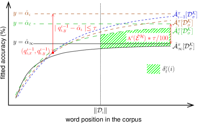
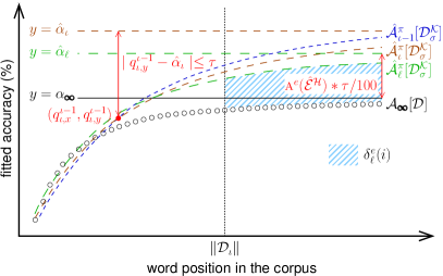
Figure 7: Computing the convergence (resp. error) accuracy for a convergence (resp. error) threshold $\tau$.

In practice, although we are interested in high values, it should be borne in mind that low accuracy does not necessarily imply a poor approximation process. Since the computationally more efficient runs are associated with larger convergence (resp. error) distances between epochs, it is more likely that it is in those runs where the divergences from the limit (resp. learning) curve will be smaller. In other words, runs with small rcs could eventually reach low accuracies, thus justifying the need for formalizing the concept of performance. As for accuracy, we differentiate between convergence and error performances to refer to the approximations of the limit and learning curves, respectively.

Definition 11.

(Relative convergence and error performance) Let $\hat{\mathcal{E}}^{\mathcal{H}}\in\mathcal{L}^{\Lambda}_{\Gamma}[{\mathcal{A}}^{\pi}[\mathcal{D}^{\mathcal{K}}_{\sigma}],\tau]$ be. We define its relative convergence (resp. relative error) performance as

$$\mbox{\sc rp}^{c}(\hat{\mathcal{E}}^{\mathcal{H}})\;\;(\mbox{resp. }\mbox{\sc rp}^{e}(\hat{\mathcal{E}}^{\mathcal{H}})):=\frac{\mbox{\sc a}^{c}(\hat{\mathcal{E}}^{\mathcal{H}})\;\;(\mbox{resp. }\mbox{\sc a}^{e}(\hat{\mathcal{E}}^{\mathcal{H}}))}{\mbox{\sc rc}(\hat{\mathcal{E}}^{\mathcal{H}})}\in[0,100]$$ (24)

Intuitively, the lower the rp in either of its interpretations, the more we could argue that an alternative approximation strategy should be considered. We are therefore interested in rps as close as possible to 100.

6 The experiments

As said, they focus on learners for ml-based tagger generation, a demanding task in nlp. We thus need to introduce the linguistic resources and the testing space.

6.1 The linguistics resources

Corpora and pos tagger generators are selected from the most popular ones, as training data and learners respectively, the former together with their tag-sets:

1. The section of the wsj in the penn treebank (Marcus et al., 1999), of over 1,170,000 words.

2. The Freiburg-Brown (frown) of American English (Hinrichs et al., 2010), of over 1,165,000 words.

penn is annotated with pos tags and syntactic structures. By stripping it of the latter, it can be used to train pos taggers. To ensure well-balanced corpora, we have scrambled them at sentence level before testing.

We focus on models built from supervised learning, which make it possible to work with predefined tag-sets, thereby facilitating both the evaluation and the comprehension of the results:

1. In the category of stochastic methods and representing the hidden Márkov models (hmms), we chose tnt (Brants, 2000). We also include the treetagger (Schmid, 1994), which uses decision trees to generate the hmm, and morfette (Chrupala et al., 2008), an averaged perceptron approach (Collins, 2002). To illustrate the maximum entropy models (mems), mxpost (Ratnaparkhi, 1996) and opennlp maxent (Toutanova et al., 2003). Finally, the stanford pos tagger (Toutanova et al., 2003) combines features of hmms and mems using a conditional Márkov model.

2. Under the heading of other approaches we consider fntbl (Ngai and Florian, 2001), an update of brill (Brill, 1995), as example of transformation-based learning. As memory-based method we take the memory-based tagger (mbt) (Daelemans et al., 1996), while svmtool (Giménez and Márquez, 2004) illustrates the behaviour with respect to support vector machines. We also use a perceptron-based training strategy with look-ahead, lapos (Tsuruoka et al., 2011).

This all ensures a good coverage of the linguistic resources for testing our proposal.

6.2 The testing space

We consider a collection ${\mathcal{L}}$ of local testing frames, with an entry for each combination of corpus and tagger. For each of these structures ${\mathcal{L}}^{\Lambda}_{\Gamma}[\mathcal{A}^{\pi}[\mathcal{D}^{\mathcal{K}}_{\sigma}],\tau]$, the size of the kernel $\mathcal{K}$ and the step function $\sigma$ are fixed to $5*10^{3}$, while a power law family parameterizable by the trust region method (Branch et al., 1999) is chosen as accuracy pattern $\pi$. The wlevel of the runs is calculated from the values proposed in (Vilares et al., 2017): $\nu=2*10^{-5}$, $\varsigma=1$ and $\lambda=5$. With respect to $\Gamma$, it includes both canonical and fixed anchoring. The proximity conditions are taken from $\Lambda=\{\mathcal{H}_{a},\mathcal{H}_{r}\}$, as defined above. Since the asymptotic backbone of any of the runs concerned is decreasing, the applicability of $\mathcal{H}_{a}$ is guaranteed and these local testing frames are well-defined. Whatever the learning trace $\mathcal{A}^{\pi}[\mathcal{D}^{\mathcal{K}}_{\sigma}]$, we will consider as reference for testing purposes a horizon of $160$ real observations provided by an omniscient oracle.

Having defined the testing structure, we address three aspects supporting the significance of the trials. The first relates to the exploitation of the training resources. Thus, as phrases are the smallest grammatical units with specific sense, samples should be aligned to the sentential distribution of the text. The second concerns the utility of the generated models, which depends on both the quality metrics being well-defined within the scope of the corpora and the reduction of variability phenomena. Finally, we tackle model optimization, i.e. the anchoring setting in each run.

6.2.1 Sampling fitting to sentence level and stability

We then need to adapt the learning schema. Given a corpus $\mathcal{D}$ with kernel $\mathcal{K}$ and a step function $\sigma$, we build the individuals $\{\mathcal{D}_{i}\}_{i\in\mathbb{N}}$ with ${\mathcal{D}}_{i}:=\left\llbracket{\mathcal{W}}_{i}\right\rrbracket$ such that

$$\begin{array}[]{l}{\mathcal{W}}_{1}:={\mathcal{K}}\mbox{ and }{\mathcal{W}}_{i}:={\mathcal{W}}_{i-1}\cup{\mathcal{I}}_{i},\;\mathcal{I}_{i}\subset{\mathcal{D}}\setminus{\mathcal{W}}_{i-1},\;\left\|{\mathcal{I}}_{i}\right\|:=\sigma(i),\;\forall i\geq 2\end{array}$$ (25)

where $\left\llbracket{\mathcal{W}}_{i}\right\rrbracket$ denotes the minimal set of sentences including the words in ${\mathcal{W}}_{i}$. This has no impact on our foundations and allows us to reap the maximum from training. Following (Daelemans et al., 1996; Giesbrecht and Evert, 2009), $10$-fold cross validation confers stability on our measures.

6.2.2 Parameter tuning

As the speed of convergence relies on the anchoring used, fine-tuning is required to select a configuration close to the most efficient one and provide credibility to the tests when the strategy is parameterizable, which is what happens with fixed anchors. Given a local testing frame $\mathcal{L}^{\Lambda}_{\Gamma}[{\mathcal{A}}^{\pi}[\mathcal{D}^{\mathcal{K}}_{\sigma}],\tau]$, the way to do it is by choosing the optimal look-ahead for a value 100, namely the one with lowest rc. Moreover, as we will see, it is only necessary to focus on runs using the absolute proximity condition ${\mathcal{H}}_{a}$.

To this end, the potential look-aheads are studied in order of increasing size, which is the same as saying that they are explored according to their corresponding put, in decreasing order. For a uniform and complete monitoring of the procedure, its codomain [0,100] is covered with step 10. We then compare the rc of the runs using the minimal look-aheads corresponding to such a sequence of tentative puts.

Given $\zeta$ a tentative put for a run $[{\mathcal{A}}^{\pi}[{\mathcal{D}}^{\mathcal{K}}_{\sigma}],\tau,{\mathcal{H}}_{a}]$, a candidate $[\hat{\mathcal{A}}^{\stackrel{{\scriptstyle 100,\iota}}{{\pi}}}[{\mathcal{D}}^{\mathcal{K}}_{\sigma}],\tau,{\mathcal{H}}_{a}]$ is generated from its minimal look-ahead $\iota$ and the rc calculated. The process is repeated for the next put until we locate the lowest rc. Hence, it is enough to identify the run associated to the turning point in such a rc sequence because, with respect to an increasing look-ahead, the performance is also increasing until reaching its maximum and then begins a decreasing trend. On this basis and to reduce the impact of irregularities, we chose that from which the window of increasing rcs is the largest one. So, it is hoped that the look-ahead is optimal with an error margin of 10% regarding the put metric.

6.3 The testing strategy

We do so according to the goals of our testing frame. That way, the cost of ensuring the completeness for $\mathcal{H}_{a}$ via fixed anchors is given by comparing within ${\mathcal{L}}$ the rc then applicable and the one estimated for similar runs when no anchoring or alternative canonical technique are used. These runs through ${\mathcal{L}}$ are hereafter referred to as ${\mathcal{L}}_{\mbox{\sc rc}}$ and do not include the baseline ones.

To balance costs and benefits of ${\mathcal{H}}_{a}$ against ${\mathcal{H}}_{r}$, we contrast the rp in its two interpretations – $\mbox{\sc rp}^{c}$ and $\mbox{\sc rp}^{e}$ – when applying the former on a run in ${\mathcal{L}}$ with fixed anchors, and when no or canonical anchors is used for its dissimilar ones. We exclude the dissimilar run with fixed anchor because Theorem 9 makes it clear that the only practical interest of this anchoring technique is to provide completeness for ${\mathcal{H}}_{a}$. Such runs through ${\mathcal{L}}$ are hereafter referred to as ${\mathcal{L}}_{\mbox{\sc rp}}$, including the baseline ones.

Table 1: rc monitoring in ${\mathcal{L}}_{\mbox{\sc rc}}$

			$\tau$		No anchor $+\;{\mathcal{H}}_{a}$						Canonical $+\;{\mathcal{H}}_{a}$						Fixed $+\;{\mathcal{H}}_{a}$
					plevel		clevel		rc		plevel		clevel		rc		put		$\ell_{o}$		plevel		clevel		rc
frown	fntbl		1.50		55		58		1.00		59		77		1.33		89.38		6		55		100		1.72
	lapos		1.27		18		46		1.00		18		71		1.54		64.86		18		18		80		1.74
	maxent		1.70		32		49		1.00		32		83		1.69		16.83		52		32		94		1.92
	mbt		1.95		43		51		1.00		51		86		1.69		29.40		43		43		98		1.92
	morfette		1.43		20		48		1.00		20		75		1.56		69.71		19		20		95		1.98
	mxpost		2.84		22		30		1.00		22		31		1.03		75.63		11		22		59		1.97
	stanford		1.91		24		36		1.00		29		72		2.00		78.29		12		24		82		2.28
	svmtool		1.41		41		52		1.00		46		89		1.71		76.02		10		41		92		1.77
	tnt		1.51		19		41		1.00		19		73		1.78		45.41		32		19		86		2.10
penn	mbt		1.66		15		39		1.00		15		85		2.18		39.50		44		15		98		2.51
	mxpost		1.40		17		28		1.00		17		50		1.79		18.73		37		17		57		2.04
	svmtool		1.25		26		31		1.00		26		66		2.13		29.69		47		26		87		2.81

Table 2: $\mbox{\sc rp}^{c}$ monitoring in ${\mathcal{L}}_{\mbox{\sc rp}}$

			$\tau$		No anchor $+\;{\mathcal{H}}_{r}$										Canonical $+\;{\mathcal{H}}_{r}$										Fixed $+\;{\mathcal{H}}_{a}$
					plevel		clevel		$\mbox{\bf{a}}^{c}$		rc		$\mbox{\bf{rp}}^{c}$		plevel		clevel		$\mbox{\bf{a}}^{c}$		rc		$\mbox{\bf{rp}}^{c}$		put		$\ell_{o}$		plevel		clevel		$\mbox{\bf{a}}^{c}$		rc		$\mbox{\bf{rp}}^{c}$
frown	fntbl		4.26		55		58		14.39		1.00		14.39		59		60		16.42		1.03		15.88		89.38		6		55		100		4.24		1.72		2.46
	lapos		3.47		18		46		6.15		1.00		6.15		18		46		6.88		1.00		6.88		64.86		18		18		80		8.38		1.74		4.82
	maxent		4.42		32		49		4.03		1.00		4.03		32		50		6.55		1.02		6.42		16.83		52		32		94		3.02		1.92		1.57
	mbt		4.78		43		51		3.02		1.00		3.02		51		52		10.66		1.02		10.45		29.40		43		43		98		1.11		1.92		0.58
	morfette		3.67		20		48		6.02		1.00		6.02		20		48		6.83		1.00		6.83		69.71		19		20		95		6.98		1.98		3.53
	mxpost		6.28		22		30		1.81		1.00		1.81		22		30		0.85		1.00		0.85		75.63		11		22		59		6.73		1.97		3.42
	stanford		4.31		24		36		7.88		1.00		7.88		29		38		16.01		1.06		15.16		78.29		12		24		82		5.33		2.28		2.34
	svmtool		3.82		41		52		13.89		1.00		13.89		46		53		16.50		1.02		16.19		76.02		10		41		92		7.09		1.77		4.01
	tnt		3.69		19		41		5.45		1.00		5.45		19		43		9.65		1.05		9.20		45.41		32		19		86		5.77		2.10		2.75
penn	mbt		3.72		15		39		18.89		1.00		18.89		15		39		5.96		1.00		5.96		39.50		44		15		98		12.85		2.51		5.11
	mxpost		3.34		17		28		2.22		1.00		2.22		17		29		4.40		1.04		4.25		18.73		37		17		57		14.70		2.04		7.22
	svmtool		2.64		26		31		23.09		1.00		23.09		26		35		28.46		1.13		25.20		29.69		47		26		87		22.94		2.81		8.18

Table 3: $\mbox{\sc rp}^{e}$ monitoring in ${\mathcal{L}}_{\mbox{\sc rp}}$

			$\tau$		No anchor $+\;{\mathcal{H}}_{r}$										Canonical $+\;{\mathcal{H}}_{r}$										Fixed $+\;{\mathcal{H}}_{a}$
					plevel		clevel		$\mbox{\bf{a}}^{e}$		rc		$\mbox{\bf{rp}}^{e}$		plevel		clevel		$\mbox{\bf{a}}^{e}$		rc		$\mbox{\bf{rp}}^{e}$		put		$\ell_{o}$		plevel		clevel		$\mbox{\bf{a}}^{e}$		rc		$\mbox{\bf{rp}}^{e}$
frown	fntbl		4.26		55		58		14.39		1.00		14.39		59		60		16.42		1.03		15.88		89.38		6		55		100		5.09		1.72		2.95
	lapos		3.47		18		46		6.15		1.00		6.15		18		46		6.88		1.00		6.88		64.86		18		18		80		8.38		1.74		4.82
	maxent		4.42		32		49		4.03		1.00		4.03		32		50		6.55		1.02		6.42		16.83		52		32		94		5.23		1.92		2.73
	mbt		4.78		43		51		3.02		1.00		3.02		51		52		10.66		1.02		10.45		29.40		43		43		98		1.46		1.92		0.76
	morfette		3.67		20		48		6.02		1.00		6.02		20		48		6.83		1.00		6.83		69.71		19		20		95		6.98		1.98		3.53
	mxpost		6.28		22		30		1.91		1.00		1.91		22		30		2.62		1.00		2.62		75.63		11		22		59		6.73		1.97		3.42
	stanford		4.31		24		36		7.88		1.00		7.88		29		38		16.01		1.06		15.16		78.29		12		24		82		5.33		2.28		2.34
	svmtool		3.82		41		52		13.89		1.00		13.89		46		53		16.50		1.02		16.19		76.02		10		41		92		7.09		1.77		4.01
	tnt		3.69		19		41		5.45		1.00		5.45		19		43		9.65		1.05		9.20		45.41		32		19		86		5.77		2.10		2.75
penn	mbt		3.72		15		39		18.89		1.00		18.89		15		39		7.80		1.00		7.80		39.50		44		15		98		12.85		2.51		5.11
	mxpost		3.34		17		28		5.05		1.00		5.05		17		29		4.95		1.04		4.78		18.73		37		17		57		14.70		2.04		7.22
	svmtool		2.64		26		31		23.09		1.00		23.09		26		35		28.46		1.13		25.20		29.69		47		26		87		22.94		2.81		8.18

Finally, in order to assess the stability of using ${\mathcal{H}}_{a}$ via fixed anchoring against look-ahead variations, we shall simply extend the set $\Gamma$ of anchorings in each local testing frame $\mathcal{L}^{\Lambda}_{\Gamma}[{\mathcal{A}}^{\pi}[\mathcal{D}^{\mathcal{K}}_{\sigma}],\tau]$, to include a selection of representative look-aheads. The runs involved in this study through ${\mathcal{L}}$ will be referred to as ${\mathcal{L}}_{\mbox{\sc rp}_{\ell}}$.

6.4 The analysis of the results

The detail of the monitoring is compiled separately for ${\mathcal{L}}_{\mbox{\sc rc}}$ (resp. ${\mathcal{L}}_{\mbox{\sc rp}}$ and ${\mathcal{L}}_{\mbox{\sc rp}_{\ell}}$) in Table 1 (resp. Tables 2-3 and 4-5) along with its plevel. We also include the clevel for each run, as well as its rc (resp. $\mbox{\sc a}^{c}$ and $\mbox{\sc rp}^{c}$, and $\mbox{\sc a}^{e}$ and $\mbox{\sc rp}^{e}$) value, which is better the closer it comes to 1 (resp. to 100). When using a fixed anchoring with value $\beta=100$, the look-ahead is also visualized, together with the associated put in the case of the optimal value $\ell_{o}$. These values are expressed to two decimal places because of space limitations, using bold (resp. italic) fonts to mark the best results among all the (resp. baseline) runs, while all the calculations have been done to six decimal places of precision. Absent from these tables are the local testing frames whose baselines show increasing asymptotic backbones, as with fntbl, lapos, maxent, morfette, stanford, tnt and treetagger trained on penn. We also discard those with any run converging beyond the boundaries of the training corpora, as with treetagger on frown.

6.4.1 Evaluating the cost of using ${\mathcal{H}}_{a}$ via fixed anchoring

The benchmark measure is now rc, whose values are compiled in Table 1 and illustrated in the left-most diagram of Fig. 8 for the set ${\mathcal{L}}_{\mbox{\sc rc}}$ of significant runs for this issue. Note that the sole aim of the estimates for the canonical technique is to illustrate the smaller impact of using ${\mathcal{H}}_{a}$ with a less invasive anchoring where possible, because in no way does the latter guarantee the completeness of such a proximity criterion.

In greater detail, rcs range from 1 for the baselines – anchor-free runs – to 2.81 for svmtool on penn if fixed anchors are considered. In percentages, 77.78% of these values are less than 2, in an interval $[1,\infty)$ of possible costs. Analyzing each anchoring approach, this ratio grows to 100% for the baselines, dropping to 75% for those applying a canonical one and to 58.33% for the fixed strategy with optimal look-ahead. The best score is for anchor-free runs in all local testing frames, while canonical anchors always provide the second best. Taking into account that convergence speed and relative cost are proportional, these results exemplify Theorem 9. Specifically, they support both the greater computational complexity of applying fixed anchors and the superiority of anchor-free runs when the impact of irregularities on the learning process is limited.

6.4.2 Evaluating the costs and benefits of using ${\mathcal{H}}_{a}$ against ${\mathcal{H}}_{r}$

Our metric is now $\mbox{\sc rp}^{c}$ (resp. $\mbox{\sc rp}^{e}$), whose values are compiled in Table 2 (resp. Table 3) and illustrated in the left-most (resp. right-most) diagram of Fig. 9 for the set ${\mathcal{L}}_{\mbox{\sc rp}}$ of significant runs for this issue, as regards the treatment of convergence (resp. error) thresholds. Note that most of these two tables are identical, just 22.2% of the runs have different values, which we have underlined so they can be easily distinguished. The origin of this behaviour is the matching in most of the runs of the values for $\mbox{\sc a}^{c}$ and $\mbox{\sc a}^{e}$. This, in turn, is a consequence of the fact that when the impact of irregularities in the learning process is limited, the maximum divergence values considered for their calculation often occur at the asymptotic level and, therefore, coincide.

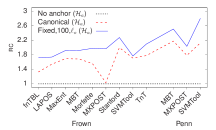
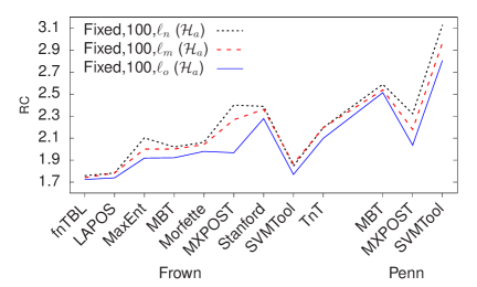
Figure 8: rc values for runs in ${\mathcal{L}}_{\mbox{\sc rc}}$ and ${\mathcal{L}}_{\mbox{\sc rp}_{\ell}}$ (look-ahead $\imath$, value $\beta=100$).

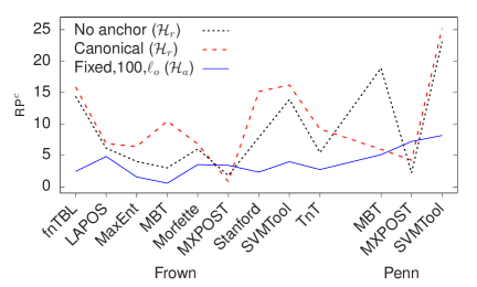
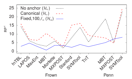
Figure 9: $\mbox{\sc rp}^{c}$ and $\mbox{\sc rp}^{e}$ values for runs in ${\mathcal{L}}_{\mbox{\sc rp}}$.

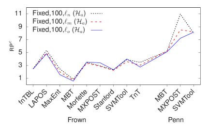
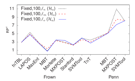
Figure 10: $\mbox{\sc rp}^{c}$ and $\mbox{\sc rp}^{e}$ values for runs in ${\mathcal{L}}_{\mbox{\sc rp}_{\ell}}$ (look-ahead $\imath$, value $\beta=100$).

In greater detail, anchor-free runs with ${\mathcal{H}}_{r}$ present the (resp. second) best $\mbox{\sc rp}^{c}$ and $\mbox{\sc rp}^{e}$ values in only one (resp. in ten) local testing frames, which corresponds to mbt on penn. Regarding the use of fixed anchors with ${\mathcal{H}}_{a}$, it turns out to be the (resp. second) best choice in two (resp. in no) cases, mxpost in both frown and penn. In all other local testing frames, the canonical anchoring with ${\mathcal{H}}_{r}$ achieves the (resp. second) best results. Overall, as one would expect from its ability to adapt dynamically to the evolution of the learning process, the best performances come from the use of canonical anchors on ${\mathcal{H}}_{r}$. On the other hand, the strong static control imposed by the fixed ones to ensure the completeness for ${\mathcal{H}}_{a}$ should relegate their use to situations where we have no information about the magnitude of the irregularities and the monotonicity – increasing or decreasing – of the learning trace involved, or we simply need to ensure an absolute threshold.

6.4.3 Stability of using ${\mathcal{H}}_{a}$ via fixed anchoring against look-ahead variations

Although the results above illustrate the application of proximity conditions based on absolute thresholds, they were obtained from runs with fixed anchors and an optimal look-ahead $\ell_{o}$ resulting from a tuning process. The aim therefore is now to determine the real impact of such a process on run performance. In this context, we extend the set $\Gamma$ of anchorings in each local testing frame $\mathcal{L}^{\Lambda}_{\Gamma}[{\mathcal{A}}^{\pi}[\mathcal{D}^{\mathcal{K}}_{\sigma}],\tau]$ with the fixed ones of value $\beta=100$ and null look-ahead $\ell_{n}$, and also $\ell_{m}:=\ell_{o}/2$. As $\ell_{o}$ is assumed to provide the best convergence speed for the proximity condition ${\mathcal{H}}_{a}$ in an increasing setting sequence, $\ell_{n}$ should supply the lowest one and $\ell_{m}$ intermediate ones. The monitoring of set ${\mathcal{L}}_{\ell}$, which brings the significant runs for this issue, is compiled (resp. illustrated) respectively for $\mbox{\sc rp}^{c}$ and $\mbox{\sc rp}^{e}$ in Tables 4 (resp. in the left-most diagram of Fig. 10) and 5 (resp. in the right-most diagram of Fig. 10). These tables also include the rc scores, which are illustrated separately in the right-most diagram of Fig. 8, and most of their entries are identical as for runs in ${\mathcal{L}}_{\mbox{\sc rp}}$. Specifically, only 22.2% of the $\mbox{\sc rp}^{c}$ and $\mbox{\sc rp}^{e}$ values are different, and we have again used underlined text to highlight them.

Table 4: $\mbox{\sc rp}^{c}$ monitoring in ${\mathcal{L}}_{\mbox{\sc rp}_{\ell}}$

			$\tau$		Fixed $+\;{\mathcal{H}}_{a}$														Fixed $+\;{\mathcal{H}}_{a}$												Fixed $+\;{\mathcal{H}}_{a}$
					put		$\ell_{o}$		plevel		clevel		$\mbox{\bf{a}}^{c}$		rc		$\mbox{\bf{rp}}^{c}$		$\ell_{m}$		plevel		clevel		$\mbox{\bf{a}}^{c}$		rc		$\mbox{\bf{rp}}^{c}$		$\ell_{n}$		plevel		clevel		$\mbox{\bf{a}}^{c}$		rc		$\mbox{\bf{rp}}^{c}$
frown	fntbl		4.26		89.38		6		55		100		4.24		1.72		2.46		3		55		101		4.31		1.74		2.47		0		55		102		4.37		1.76		2.49
	lapos		3.47		64.86		18		18		80		8.38		1.74		4.82		9		18		82		8.83		1.78		4.95		0		18		82		9.55		1.78		5.36
	maxent		4.42		16.83		52		32		94		3.02		1.92		1.57		26		32		98		4.00		2.00		2.00		0		32		103		5.17		2.10		2.46
	mbt		4.78		29.40		43		43		98		1.11		1.92		0.58		22		43		102		1.40		2.00		0.70		0		43		103		1.76		2.02		0.87
	morfette		3.67		69.71		19		20		95		6.98		1.98		3.53		10		20		98		6.85		2.04		3.35		0		20		99		7.18		2.06		3.48
	mxpost		6.28		75.63		11		22		59		6.73		1.97		3.42		6		22		68		6.49		2.27		2.86		0		22		72		7.07		2.40		2.95
	stanford		4.31		78.29		12		24		82		5.33		2.28		2.34		6		24		85		5.30		2.36		2.24		0		24		86		5.50		2.39		2.30
	svmtool		3.82		76.02		10		41		92		7.09		1.77		4.01		5		41		97		6.71		1.87		3.60		0		41		96		7.22		1.85		3.91
	tnt		3.69		45.41		32		19		86		5.77		2.10		2.75		16		19		90		6.69		2.20		3.05		0		19		90		7.65		2.20		3.49
penn	mbt		3.72		39.50		44		15		98		12.85		2.51		5.11		22		15		99		13.26		2.54		5.22		0		15		101		13.47		2.59		5.20
	mxpost		3.34		18.73		37		17		57		14.70		2.04		7.22		19		17		61		18.58		2.18		8.53		0		17		65		25.46		2.32		10.97
	svmtool		2.64		29.69		47		26		87		22.94		2.81		8.18		24		26		92		24.38		2.97		8.21		0		26		97		25.10		3.13		8.02

Table 5: $\mbox{\sc rp}^{e}$ monitoring in ${\mathcal{L}}_{\mbox{\sc rp}_{\ell}}$

			$\tau$		Fixed $+\;{\mathcal{H}}_{a}$														Fixed $+\;{\mathcal{H}}_{a}$												Fixed $+\;{\mathcal{H}}_{a}$
					put		$\ell_{o}$		plevel		clevel		$\mbox{\bf{a}}^{c}$		rc		$\mbox{\bf{rp}}^{c}$		$\ell_{m}$		plevel		clevel		$\mbox{\bf{a}}^{c}$		rc		$\mbox{\bf{rp}}^{c}$		$\ell_{n}$		plevel		clevel		$\mbox{\bf{a}}^{c}$		rc		$\mbox{\bf{rp}}^{c}$
frown	fntbl		4.26		89.38		6		55		100		5.09		1.72		2.95		3		55		101		5.10		1.74		2.93		0		55		102		5.13		1.76		2.92
	lapos		3.47		64.86		18		18		80		8.38		1.74		4.82		9		18		82		8.83		1.78		4.95		0		18		82		9.55		1.78		5.36
	maxent		4.42		16.83		52		32		94		5.23		1.92		2.73		26		32		98		5.62		2.00		2.81		0		32		103		6.13		2.10		2.92
	mbt		4.78		29.40		43		43		98		1.46		1.92		0.76		22		43		102		2.79		2.00		1.40		0		43		103		1.76		2.02		0.87
	morfette		3.67		69.71		19		20		95		6.98		1.98		3.53		10		20		98		6.85		2.04		3.35		0		20		99		7.18		2.06		3.48
	mxpost		6.28		75.63		11		22		59		6.73		1.97		3.42		6		22		68		6.49		2.27		2.86		0		22		72		7.07		2.40		2.95
	stanford		4.31		78.29		12		24		82		5.33		2.28		2.34		6		24		85		5.30		2.36		2.24		0		24		86		5.50		2.39		2.30
	svmtool		3.82		76.02		10		41		92		7.09		1.77		4.01		5		41		97		6.71		1.87		3.60		0		41		96		7.22		1.85		3.91
	tnt		3.69		45.41		32		19		86		5.77		2.10		2.75		16		19		90		6.69		2.20		3.05		0		19		90		7.65		2.20		3.49
penn	mbt		3.72		39.50		44		15		98		12.85		2.51		5.11		22		15		99		13.26		2.54		5.22		0		15		101		13.47		2.59		5.20
	mxpost		3.34		18.73		37		17		57		14.70		2.04		7.22		19		17		61		18.58		2.18		8.53		0		17		65		25.46		2.32		10.97
	svmtool		2.64		29.69		47		26		87		22.94		2.81		8.18		24		26		92		24.38		2.97		8.21		0		26		97		25.10		3.13		8.02

In short, we find that rcs range from 1.72 for fntbl on frown with a look-ahead $\ell_{o}$, to 3.13 for svmtool on penn with $\ell_{n}$. In percentages, 36.11% of these values are less than 2, in an interval $[1,\infty)$ of possible costs. Analyzing each anchoring approach, this ratio grows to 58.33% when using $\ell_{o}$ look-aheads and drops to 25% otherwise. The best score is for $\ell_{o}$ in all local testing frames, while $\ell_{m}$ provides the second best result in all cases but one, and $\ell_{n}$ in three. Note that $\ell_{m}$ and $\ell_{n}$ obtain the same rcs for lapos and tnt in frown. This again exemplifies the conclusions of Theorem 9 about anchor categorization, this time regarding the use of look-aheads, but also illustrates the usefulness and validity of the concept of minimal look-ahead for a tentative put as a mechanism for optimizing fixed anchorings.

As for $\mbox{\sc rp}^{c}$ (resp. $\mbox{\sc rp}^{e}$), the optimal look-ahead $\ell_{o}$ gives the best values in four (resp. five) cases, while $\ell_{m}$ and $\ell_{n}$ do so in two (resp. three) and six (resp. four) ones, respectively. Regarding the second best choice, it corresponds to $\ell_{o}$ in only one (resp. one) case and in six (resp. five) ones to $\ell_{m}$, while anchor-free runs reach that position five (resp. six) times. Overall, the best performances seem to correspond to the absence of look-ahead, followed by those associated with the use of the mean value $\ell_{m}$ and the optimum one $\ell_{o}$, although the differences are very small as can be seen in Fig. 10. This suggests that the choice of look-ahead has a minor impact on the performance, thus allowing its use to be simplified, as it would no longer require a prior tuning phase.

7 Conclusions

We have responded to the challenge of estimating absolute convergence thresholds associated with the prediction of learning processes as a means of reducing training effort and the need for resources in the generation of ml-based systems. The goal is to get the most from a non-active adaptive sampling scheme used for that purpose, by limiting its application in time to what is strictly necessary, while avoiding the limitations of relative measures.

Our proposal proves its correctness with respect to its working hypotheses. Namely, it determines the cycle from which we can ensure that the threshold fixed by the user has been reached. Since this can only be established in practice when the successive estimates for accuracy are decreasing, the completeness of the technique is also stated. To do so, we demonstrate that it is possible to redirect the training dynamics in such a way that such a property verifies. This is achieved by properly using the concept of anchor, a conservative assessment of the final accuracy achievable by the learner, which is calculated from a sufficiently representative sample interpreted as an observation at the point of infinity for the calculation of the next estimate. Furthermore, since the primary function of anchoring is to compensate the irregularities in the learning process due to deviations in the working hypotheses, the proposal shows a good degree of robustness.

To reduce the slowdown caused on the pace of convergence by the use of anchors, we introduce a parameterizable family of these structures, categorizing them with respect to both the costs and the balance between these and their benefits. The tests, taking the generation of pos taggers in nlp as case study, corroborate our expectations. In particular, although the consideration of absolute thresholds applying our proposal entails greater computational cost, it has demonstrated its reliability and practical aplicability, providing a stable and robust way to proceed when relative estimations of the learning curve are not sufficient for the development of ml applications.

Appendix A Proofs for Subsection 4.3

A.1 Proof of Theorem 4

Since $\hat{\rho}_{i}(\infty):=\hat{\mathcal{A}}_{i}(\infty)-\hat{\alpha}_{i},\forall i>\omega$, the asymptotic backbone $\{\hat{\alpha}_{i}\}_{i>\omega}$ is decreasing iff it verifies that

$$\forall i>\omega,\;\hat{\alpha}_{i}\geq\hat{\alpha}_{i+1}\Leftrightarrow\hat{\mathcal{A}}_{i}(\infty)-\hat{\mathcal{A}}_{i+1}(\infty)\geq\hat{\rho}_{i}(\infty)-\hat{\rho}_{i+1}(\infty),\;$$ (26)

which derives immediately from Equation 11. To now complete the proof, we only need to demonstrate that $\{\hat{\alpha}_{i}\}_{i>\omega}$ converges to $\alpha_{\boldsymbol{\boldsymbol{\infty}}{}}$. As $\hat{\mathcal{A}}_{i}^{\pi}[{\mathcal{D}}^{\mathcal{K}}_{\sigma}]$ is a fitting curve for the values

$$\{[x_{j},{\mathcal{A}}_{\boldsymbol{\boldsymbol{\infty}}{}}[{\mathcal{D}}](x_{j})],\;x_{j}:=\left\|\mathcal{D}_{j}\right\|\}_{j=1}^{i}\;\cup\;\{[\infty,\hat{\mathcal{A}}_{i}(\infty)]\},\;\forall i>\omega$$ (27)

we then have that

$$\hat{\mathcal{A}}_{i}(\infty)\geq\hat{\alpha}_{i}:=\lim\limits_{x\rightarrow\infty}\hat{\mathcal{A}}_{i}^{\pi}[{\mathcal{D}}^{\mathcal{K}}_{\sigma}](x),\;\forall i>\omega$$ (28)

If we also take into account that ${\mathcal{A}}_{i}^{\pi}[{\mathcal{D}}^{\mathcal{K}}_{\sigma}]$ is a curve fitting the set

$$\{[x_{j},{\mathcal{A}}_{\boldsymbol{\boldsymbol{\infty}}{}}[{\mathcal{D}}](x_{j})],\;x_{j}:=\left\|\mathcal{D}_{j}\right\|\}_{j=1}^{i}\;\cup\;\{[\infty,\alpha_{i}]\},\;\forall i>\omega$$ (29)

with anchors verifying the Equation 10, we then have that

$$\hat{\mathcal{A}}_{i}(\infty)\geq\hat{\alpha}_{i}:=\lim\limits_{x\rightarrow\infty}\hat{\mathcal{A}}_{i}^{\pi}[{\mathcal{D}}^{\mathcal{K}}_{\sigma}](x)\geq\alpha_{i},\;\forall i>\wp$$ (30)

from which

$$\lim\limits_{i\rightarrow\infty}\hat{\mathcal{A}}_{i}(\infty)\geq\lim\limits_{i\rightarrow\infty}\hat{\alpha}_{i}\geq\lim\limits_{i\rightarrow\infty}\alpha_{i}=\alpha_{\boldsymbol{\boldsymbol{\infty}}{}}$$ (31)

Moreover, the impact of the singularity $\hat{\mathcal{A}}_{\infty}^{\pi}[{\mathcal{D}}^{\mathcal{K}}_{\sigma}](\infty)$ in the generation of the learning trends $\{\hat{\mathcal{A}}_{i}[{\mathcal{D}}^{\mathcal{K}}_{\sigma}]\}_{i>\omega}$ decreases as the level ascends. Namely, $\alpha_{\boldsymbol{\boldsymbol{\infty}}{}}$ is a supremum for $\{\hat{\alpha}_{i}\}_{i>\omega}$ and $\lim\limits_{i\rightarrow\infty}\hat{\alpha}_{i}=\lim\limits_{i\rightarrow\infty}\alpha_{i}=\alpha_{\boldsymbol{\boldsymbol{\infty}}{}}$, which proves the thesis.

A.2 Proof of Theorem 5

Let $\{\alpha_{i}\}_{i\in\mathbb{N}}$ be the backbone for the reference $[{\mathcal{A}}^{\pi}[{\mathcal{D}}^{\mathcal{K}}_{\sigma}],\omega]$ of $\hat{\mathcal{A}}^{\pi}[{\mathcal{D}}^{\mathcal{K}}_{\sigma}]$ and $\wp$ the plevel of the latter. By Theorem 4, it is enough to prove that its hypotheses verify. Focusing on Equation 10, let us first assume $i=\omega+1$. Since by hypothesis $\{\alpha_{i}\}_{i\in\mathbb{N}}$ is decreasing, we conclude that

$$\hat{\mathcal{A}}_{\omega+1}(\infty):=\alpha_{\omega}\geq\alpha_{\omega+1}$$ (32)

Let us now assume that $i>\omega+1$, as $\{\alpha_{i}\}_{i\in\mathbb{N}}$ is decreasing, Theorem 1 proves that $\hat{\alpha}_{\omega+i}\geq\alpha_{\omega+i},\forall i>\omega$, from which we derive that

$$\hat{\mathcal{A}}_{i+1}(\infty):=\hat{\alpha}_{i}\geq\alpha_{i}\geq\alpha_{i+1}$$ (33)

and we can then affirm that $\hat{\mathcal{A}}_{i}(\infty)\geq\alpha_{i},\;\forall i>\wp\geq\omega$, completing the proof in this case.

Regarding the compliance of the condition referred in Equation 11, as $\hat{\rho}_{i}(\infty):=\hat{\mathcal{A}}_{i}(\infty)-\hat{\alpha}_{i}$, demonstrating the inequality

$$\hat{\mathcal{A}}_{i}(\infty)-\hat{\mathcal{A}}_{i+1}(\infty)\geq\hat{\rho}_{i}(\infty)-\hat{\rho}_{i+1}(\infty),\;\forall i>0+\omega=\omega$$ (34)

which is to prove $\hat{\alpha}_{i}\geq\hat{\alpha}_{i+1},\forall i>\omega$. As this was stated in Theorem 1, we conclude the thesis.

A.3 Proof of Theorem 6

By Theorem 4, as $\{\hat{\mathcal{A}}_{i}^{\beta}(\infty)\}_{i>\omega}$ is convergent to $\beta$, it is enough to prove that its hypotheses verify. To this end, the condition in Equation 10 becomes trivial because the plevel $\wp$ is the first level after the working one $\omega$ from which the asymptotic backbone is below 100, and therefore

$$\hat{\mathcal{A}}_{i}^{\beta}(\infty):=\beta\geq 100\geq\alpha_{i},\;\forall i>\wp$$ (35)

With respect to the condition in Equation 11, given that $\hat{\mathcal{A}}_{i}^{\stackrel{{\scriptstyle\beta}}{{\pi}}}[{\mathcal{D}}^{\mathcal{K}}_{\sigma}]$ is a curve fitting

$$\{[x_{j},{\mathcal{A}}_{\boldsymbol{\boldsymbol{\infty}}{}}[{\mathcal{D}}](x_{j})],\;x_{j}:=\left\|\mathcal{D}_{j}\right\|\}_{j=1}^{i}\;\cup\;\{[\infty,\beta]\}$$ (36)

and the observations of the first set are lower or equal than $100\leq\beta$, we have that the asymptotic backbone $\{\hat{\alpha}_{i}^{\beta}\}_{i>\omega}$ of $\hat{\mathcal{A}}^{\stackrel{{\scriptstyle\beta}}{{\pi}}}[{\mathcal{D}}^{\mathcal{K}}_{\sigma}]$ is never greater than $\beta$ and therefore the residuals $\{\hat{\rho}_{i}^{\beta}(\infty)\}_{i>\omega}$ are invariably positive or null, because

$$\hat{\rho}_{i}^{\beta}(\infty):=\hat{\mathcal{A}}_{i}^{\beta}(\infty)-\hat{\alpha}_{i}^{\beta}:=\beta-\hat{\alpha}_{i}^{\beta}$$ (37)

As $\{[x_{i},{\mathcal{A}}_{\boldsymbol{\boldsymbol{\infty}}{}}[{\mathcal{D}}](x_{i})],\;x_{i}:=\left\|\mathcal{D}_{i}\right\|\}_{i\in\mathbb{N}}$ is increasing, its impact on the generation of the learning trends $\{\hat{\mathcal{A}}_{i}^{\stackrel{{\scriptstyle\beta}}{{\pi}}}[{\mathcal{D}}^{\mathcal{K}}_{\sigma}]\}_{i>\omega}$ grows with each sample and therefore the absolute value of the residuals $\{\hat{\rho}_{i}^{\beta}(\infty)\}_{i>\omega}$ also. We then derive that:

$$\hat{\mathcal{A}}_{i}^{\beta}(\infty)-\hat{\mathcal{A}}_{i+1}^{\beta}(\infty)=0\geq\hat{\rho}_{i}^{\beta}(\infty)-\hat{\rho}_{i+1}^{\beta}(\infty),\;\forall i>\omega$$ (38)

and Equation 11 verifies.

A.4 Proof of Theorem 7

By Theorem 6, as ${\mathcal{A}}^{\pi}[{\mathcal{D}}^{\mathcal{K}}_{\sigma}]$ is a learning trace with fixed anchor, its asymptotic backbone $\{\alpha_{i}\}_{i>\omega}$ is decreasing and the thesis is proved applying the same reasoning used in Theorem 3.

A.5 Proof of Theorem 8

Following Theorem 4, as $\{\hat{\mathcal{A}}_{i}^{\beta,\ell}(\infty)\}_{i>\omega}$ converges to $\hat{\mathcal{A}}_{\omega+\ell}^{\beta,\ell}(\infty)$, it is enough to prove that its hypotheses verify. With regard to the condition expressed in Equation 10, let us assume $\{\hat{\mathcal{A}}_{i}^{\stackrel{{\scriptstyle\beta}}{{\pi}}}[{\mathcal{D}}^{\mathcal{K}}_{\sigma}]\}_{i>\omega}$ the fixed anchoring learning trace of value $\beta$ for ${\mathcal{A}}^{\pi}[{\mathcal{D}}^{\mathcal{K}}_{\sigma}]$. As its asymptotic backbone $\{\hat{\alpha}_{i}^{\beta}\}_{i>\omega}$ is decreasing and $\wp\geq\omega$, we have that, $\forall i\geq\wp+\ell+1$

$$\hat{\alpha}_{\wp+\ell}^{\beta}\geq\hat{\alpha}_{i}^{\beta}:=\lim\limits_{x\rightarrow\infty}\hat{\mathcal{A}}_{i}^{\stackrel{{\scriptstyle\beta}}{{\pi}}}[{\mathcal{D}}^{\mathcal{K}}_{\sigma}](x)$$ (39)

where $\hat{\mathcal{A}}_{i}^{\stackrel{{\scriptstyle\beta}}{{\pi}}}[{\mathcal{D}}^{\mathcal{K}}_{\sigma}]$ is a curve fitting the set of values

$$\{[x_{j},{\mathcal{A}}_{\boldsymbol{\boldsymbol{\infty}}{}}[{\mathcal{D}}](x_{j})]\}_{j=1}^{i}\;\cup\;\{[\infty,\hat{\mathcal{A}}_{i}^{\beta}(\infty)]\}=\{[x_{j},{\mathcal{A}}_{\boldsymbol{\boldsymbol{\infty}}{}}[{\mathcal{D}}](x_{j})]\}_{j=1}^{i}\;\cup\;\{[\infty,\beta]\},\;x_{j}:=\left\|\mathcal{D}_{j}\right\|$$ (40)

Since ${\mathcal{A}}_{i}^{\pi}[{\mathcal{D}}^{\mathcal{K}}_{\sigma}]$ is a curve fitting the first set $\{[x_{j},{\mathcal{A}}_{\boldsymbol{\boldsymbol{\infty}}{}}[{\mathcal{D}}](x_{j})],\;x_{j}:=\left\|\mathcal{D}_{j}\right\|\}_{j=1}^{i}$ and by hypothesis $\beta\geq 100\geq{\mathcal{A}}_{\boldsymbol{\boldsymbol{\infty}}{}}[{\mathcal{D}}](x_{j}),\forall j\in\mathbb{N}$, we deduce that $\hat{\alpha}_{i}^{\beta}\geq\alpha_{i}$, with $\{\alpha_{i}\}_{i\in\mathbb{N}}$ the asymptotic backbone for the reference $[{\mathcal{A}}^{\pi}[{\mathcal{D}}^{\mathcal{K}}_{\sigma}],\omega]$. Taking also into account that $\lim\limits_{x\rightarrow\infty}\hat{\mathcal{A}}_{i}^{\stackrel{{\scriptstyle\beta}}{{\pi}}}[{\mathcal{D}}^{\mathcal{K}}_{\sigma}](x):=\hat{\alpha}_{i}^{\beta}$ and $\lim\limits_{x\rightarrow\infty}{\mathcal{A}}_{i}^{\pi}[{\mathcal{D}}^{\mathcal{K}}_{\sigma}](x):=\alpha_{i}$, it verifies that

$$\hat{\mathcal{A}}_{i}^{\beta,\ell}(\infty):=\hat{\alpha}_{\wp+\ell}^{\beta,\ell}:=\hat{\alpha}_{\wp+\ell}^{\beta}\geq\hat{\alpha}_{i}^{\beta}\geq\alpha_{i},\;\forall i\geq\wp+\ell+1$$ (41)

Furthermore, since $\wp$ is precisely the first level after the working one $\omega$ from which the asymptotic backbone is below 100, we deduce that

$$\hat{\mathcal{A}}_{i}^{\beta,\ell}(\infty):=\beta\geq 100\geq\alpha_{i},\;\forall\;\wp+\ell+1>i>\omega$$ (42)

and therefore $\hat{\mathcal{A}}_{i}^{\beta,\ell}(\infty)\geq\alpha_{i},\forall i>\omega$, thus matching the relationship described in Equation 10.

With respect to the condition in Equation 11, we study it separately in each interval of definition for the asymptotic backbone $\{\hat{\alpha}_{i}^{\beta,\ell}\}_{i>\omega}$. Let us first assume $\wp+\ell+1>i>\omega$. As in this case

$$\hat{\mathcal{A}}_{i}^{\beta,\ell}(\infty):=\hat{\mathcal{A}}_{i}^{\beta}(\infty):=\beta\geq 100$$ (43)

we can apply the same reasoning used in Theorem 6 to prove that $\{\hat{\alpha}_{i}^{\beta,\ell}\}_{i>\omega}$ is decreasing in that interval.

Let us now consider $i>\wp+\ell+1$. Then, $\hat{\mathcal{A}}_{i}^{\stackrel{{\scriptstyle\beta,\ell}}{{\pi}}}[{\mathcal{D}}^{\mathcal{K}}_{\sigma}]$ is here a curve fitting the collection of values

$$\{[x_{j},{\mathcal{A}}_{\boldsymbol{\boldsymbol{\infty}}{}}[{\mathcal{D}}](x_{j})]\}_{j=1}^{i}\;\cup\;\{[\infty,\hat{\mathcal{A}}_{i}^{\beta,\ell}(\infty)]\}=\{[x_{j},{\mathcal{A}}_{\boldsymbol{\boldsymbol{\infty}}{}}[{\mathcal{D}}](x_{j})]\}_{j=1}^{i}\;\cup\;\{[\infty,\hat{\alpha}_{\wp+\ell}^{\beta,\ell}]\}$$ (44)

with $x_{j}:=\left\|\mathcal{D}_{j}\right\|$. Given that the observations of the first set are always lower or equal than

$$\hat{\mathcal{A}}_{i}^{\beta,\ell}(\infty):=\hat{\alpha}_{\wp+\ell}^{\beta,\ell}:=\hat{\alpha}_{\wp+\ell}^{\beta}$$ (45)

because Theorem 6 states that $\{\hat{\alpha}_{i}^{\beta}\}_{i>\omega}$ is decreasing, the subsequence $\{\hat{\alpha}_{i}^{\beta,\ell}\}_{i>\wp+\ell+1}$ of the asymptotic backbone of $\hat{\mathcal{A}}^{\stackrel{{\scriptstyle\beta,\ell}}{{\pi}}}[{\mathcal{D}}^{\mathcal{K}}_{\sigma}]$ is never greater than $\hat{\alpha}_{\wp+\ell}^{\beta,\ell}$ and therefore the sequence of its associated residuals $\{\hat{\rho}_{i}^{\beta,\ell}(\infty)\}_{i>\wp+\ell+1}$ is invariably positive or null, because

$$\hat{\rho}_{i}^{\beta,\ell}(\infty):=\hat{\mathcal{A}}_{i}^{\beta,\ell}(\infty)-\hat{\alpha}_{i}^{\beta,\ell}:=\hat{\mathcal{A}}_{i}^{\beta,\ell}(\infty)-\lim\limits_{x\rightarrow\infty}\hat{\mathcal{A}}_{i}^{\stackrel{{\scriptstyle\beta,\ell}}{{\pi}}}[{\mathcal{D}}^{\mathcal{K}}_{\sigma}](x)$$ (46)

As $\{[x_{i},{\mathcal{A}}_{\boldsymbol{\boldsymbol{\infty}}{}}[{\mathcal{D}}](x_{i})],\;x_{i}:=\left\|\mathcal{D}_{i}\right\|\}_{i\in\mathbb{N}}$ is increasing, its impact on the generation of the learning trends $\{\hat{\mathcal{A}}_{i}^{\stackrel{{\scriptstyle\beta,\ell}}{{\pi}}}[{\mathcal{D}}^{\mathcal{K}}_{\sigma}]\}_{i>\wp+\ell+1}$ grows with each sample and therefore the absolute value of the residuals $\{\hat{\rho}_{i}^{\beta,\ell}(\infty)\}_{i>\wp+\ell+1}$ also. We then derive that:

$$\hat{\mathcal{A}}_{i}^{\beta,\ell}(\infty)-\hat{\mathcal{A}}_{i+1}^{\beta,\ell}(\infty)=0\geq\hat{\rho}_{i}^{\beta,\ell}(\infty)-\hat{\rho}_{i+1}^{\beta,\ell}(\infty),\;\forall i>\wp+\ell+1$$ (47)

and Equation 11 also verifies in the latter interval.

That way, what is lacking to match the relationship in Equation 11 on its full application domain is to demonstrate that

$$\hat{\mathcal{A}}_{\wp+\ell}^{\beta,\ell}(\infty)-\hat{\mathcal{A}}_{\wp+\ell+1}^{\beta,\ell}(\infty)\geq\hat{\rho}_{\wp+\ell}^{\beta,\ell}(\infty)-\hat{\rho}_{\wp+\ell+1}^{\beta,\ell}(\infty)$$ (48)

which is equivalent to prove that $\hat{\alpha}_{\wp+\ell}^{\beta,\ell}\geq\hat{\alpha}_{\wp+\ell+1}^{\beta,\ell}$, because $\hat{\rho}_{i}^{\beta,\ell}(\infty):=\hat{\mathcal{A}}_{i}^{\beta,\ell}(\infty)-\hat{\alpha}_{i}^{\beta,\ell}$.

From Theorem 6, $\{\hat{\alpha}_{i}^{\beta}\}_{i>\omega}$ converges decreasingly to the final accuracy $\alpha_{\boldsymbol{\boldsymbol{\infty}}{}}:=\lim\limits_{x\rightarrow\infty}{\mathcal{A}}_{\boldsymbol{\boldsymbol{\infty}}}[{\mathcal{D}}](x)$ attained from the training process. As ${\mathcal{A}}_{\boldsymbol{\boldsymbol{\infty}}{}}[{\mathcal{D}}]$ is increasing, we infer that

$${\mathcal{A}}_{\boldsymbol{\boldsymbol{\infty}}{}}[{\mathcal{D}}](x_{i})\leq\alpha_{\boldsymbol{\boldsymbol{\infty}}{}}\leq\hat{\alpha}_{\wp+\ell}^{\beta}:=\hat{\alpha}_{\wp+\ell}^{\beta,\ell},\;x_{i}:=\left\|\mathcal{D}_{i}\right\|$$ (49)

Furthermore, $\hat{\alpha}_{\wp+\ell+1}^{\beta,\ell}:=\lim\limits_{x\rightarrow\infty}\hat{\mathcal{A}}_{\wp+\ell+1}^{\stackrel{{\scriptstyle\beta,\ell}}{{\pi}}}[{\mathcal{D}}^{\mathcal{K}}_{\sigma}](x)$, where $\hat{\mathcal{A}}_{\wp+\ell+1}^{\stackrel{{\scriptstyle\beta,\ell}}{{\pi}}}[{\mathcal{D}}^{\mathcal{K}}_{\sigma}]$ is a fitting curve for the set

$$\{[x_{j},{\mathcal{A}}_{\boldsymbol{\boldsymbol{\infty}}{}}[{\mathcal{D}}](x_{j})]\}_{j=1}^{\wp+\ell}\;\cup\;\{[\infty,\hat{\mathcal{A}}_{\wp+\ell}^{\beta,\ell}(\infty)]\}=\{[x_{j},{\mathcal{A}}_{\boldsymbol{\boldsymbol{\infty}}{}}[{\mathcal{D}}](x_{j})]\}_{j=1}^{\wp+\ell}\;\cup\;\{[\infty,\hat{\alpha}_{\wp+\ell-1}^{\beta,\ell}]\}$$ (50)

with $x_{j}:=\left\|\mathcal{D}_{j}\right\|$. As we have established that the ordinates of these values are below $\hat{\alpha}_{\wp+\ell+1}^{\beta,\ell}$, we derive what we were looking for

$$\hat{\alpha}_{\wp+\ell}^{\beta,\ell}\geq\lim\limits_{x\rightarrow\infty}\hat{\mathcal{A}}_{\wp+\ell+1}^{\stackrel{{\scriptstyle\beta,\ell}}{{\pi}}}[{\mathcal{D}}^{\mathcal{K}}_{\sigma}](x):=\hat{\alpha}_{\wp+\ell+1}^{\beta,\ell}$$ (51)

thus terminating the proof.

A.6 Proof of Theorem 9

We first address the Equations 15 and 16, when no hypothesis regarding the monotony of the asymptotic backbone $\{\alpha_{i}\}_{i\in\mathbb{N}}$ associated to the reference is established. Given that the former has already been stated (Vilares et al., 2017), we focus on the second one, starting from its left-most inequality.

Let us assume $\jmath>\imath$, $\eta>\beta$ and $i\geq\wp+\jmath$, then $\hat{\alpha}_{i}^{\beta,\imath}:=\lim\limits_{x\rightarrow\infty}\hat{\mathcal{A}}_{i}^{\stackrel{{\scriptstyle\beta,\imath}}{{\pi}}}[{\mathcal{D}}^{\mathcal{K}}_{\sigma}](x)$, with $\hat{\mathcal{A}}_{i}^{\stackrel{{\scriptstyle\beta,\imath}}{{\pi}}}[{\mathcal{D}}^{\mathcal{K}}_{\sigma}]$ a fitting curve for the values

$$\{[x_{j},{\mathcal{A}}_{\boldsymbol{\boldsymbol{\infty}}{}}[{\mathcal{D}}^{\mathcal{K}}_{\sigma}](x_{j})]\}_{j=1}^{i}\;\cup\;\{[\infty,\hat{\mathcal{A}}_{i}^{\beta,\imath}(\infty)]\}=\{[x_{j},{\mathcal{A}}_{\boldsymbol{\boldsymbol{\infty}}{}}[{\mathcal{D}}^{\mathcal{K}}_{\sigma}](x_{j})]\}_{j=1}^{i}\;\cup\;\{[\infty,\hat{\alpha}_{\imath}^{\beta}]\}$$ (52)

with $x_{j}:=\left\|\mathcal{D}_{j}\right\|$. Similarly, $\hat{\alpha}_{i}^{\beta,\jmath}:=\lim\limits_{x\rightarrow\infty}\hat{\mathcal{A}}_{i}^{\stackrel{{\scriptstyle\beta,\jmath}}{{\pi}}}[{\mathcal{D}}^{\mathcal{K}}_{\sigma}](x)$, with $\hat{\mathcal{A}}_{i}^{\stackrel{{\scriptstyle\beta,\jmath}}{{\pi}}}[{\mathcal{D}}^{\mathcal{K}}_{\sigma}]$ a curve fitting

$$\{[x_{j},{\mathcal{A}}_{\boldsymbol{\boldsymbol{\infty}}{}}[{\mathcal{D}}](x_{j})],\;x_{j}:=\left\|\mathcal{D}_{j}\right\|\}_{j=1}^{i}\;\cup\;\{[\infty,\hat{\alpha}_{\jmath}^{\beta}]\}$$ (53)

where, as by Theorem 6 the sequence $\{\hat{\alpha}_{i}^{\beta}\}_{i>\omega}$ converges decreasingly to $\alpha_{\infty}=\alpha_{\boldsymbol{\boldsymbol{\infty}}{}}\geq 0$, we conclude that $\hat{\alpha}_{\imath}^{\beta}>\hat{\alpha}_{\jmath}^{\beta}$. As Theorem 8 guarantees that $\{\hat{\alpha}_{i}^{\beta,\imath}\}_{i>\omega}$ and $\{\hat{\alpha}_{i}^{\beta,\jmath}\}_{i>\omega}$ also converge decreasingly to $\alpha_{\infty}=\alpha_{\boldsymbol{\boldsymbol{\infty}}{}}\geq 0$, and $\wp\geq\omega$, we can conclude that $\mid\hat{\alpha}_{i}^{\beta,\jmath}-\alpha_{\boldsymbol{\boldsymbol{\infty}}{}}\mid\leq\mid\hat{\alpha}_{i}^{\beta,\imath}-\alpha_{\boldsymbol{\boldsymbol{\infty}}{}}\mid$. We thereby demonstrate the inequality in question.

On the other hand, $\hat{\alpha}_{i}^{\eta,\imath}:=\lim\limits_{x\rightarrow\infty}\hat{\mathcal{A}}_{i}^{\stackrel{{\scriptstyle\eta,\imath}}{{\pi}}}[{\mathcal{D}}^{\mathcal{K}}_{\sigma}](x)$, with $\hat{\mathcal{A}}_{i}^{\stackrel{{\scriptstyle\eta,\imath}}{{\pi}}}[{\mathcal{D}}^{\mathcal{K}}_{\sigma}]$ a fitting curve for the values

$$\{[x_{j},{\mathcal{A}}_{\boldsymbol{\boldsymbol{\infty}}{}}[{\mathcal{D}}](x_{j})]\}_{j=1}^{i}\;\cup\;\{[\infty,\hat{\mathcal{A}}_{i}^{\eta,\imath}(\infty)]\}=\{[x_{j},{\mathcal{A}}_{\boldsymbol{\boldsymbol{\infty}}{}}[{\mathcal{D}}](x_{j})]\}_{j=1}^{i}\;\cup\;\{[\infty,\hat{\alpha}_{\imath}^{\eta}]\}$$ (54)

where $x_{j}:=\left\|\mathcal{D}_{j}\right\|$ and $\hat{\alpha}_{i}^{\eta}:=\lim\limits_{x\rightarrow\infty}\hat{\mathcal{A}}_{i}^{\stackrel{{\scriptstyle\eta}}{{\pi}}}[{\mathcal{D}}^{\mathcal{K}}_{\sigma}](x)$, with $\hat{\mathcal{A}}_{i}^{\stackrel{{\scriptstyle\eta}}{{\pi}}}[{\mathcal{D}}^{\mathcal{K}}_{\sigma}]$ a fitting curve for the values

$$\{[x_{j},{\mathcal{A}}_{\boldsymbol{\boldsymbol{\infty}}{}}[{\mathcal{D}}](x_{j})]\}_{j=1}^{i}\;\cup\;\{[\infty,\hat{\mathcal{A}}_{i}^{\eta}(\infty)]\}=\{[x_{j},{\mathcal{A}}_{\boldsymbol{\boldsymbol{\infty}}{}}[{\mathcal{D}}](x_{j})]\}_{j=1}^{i}\;\cup\;\{[\infty,\eta]\},\;x_{j}:=\left\|\mathcal{D}_{j}\right\|$$ (55)

Similarly, $\hat{\alpha}_{i}^{\beta}:=\lim\limits_{x\rightarrow\infty}\hat{\mathcal{A}}_{i}^{\stackrel{{\scriptstyle\beta}}{{\pi}}}[{\mathcal{D}}^{\mathcal{K}}_{\sigma}](x)$, with $\hat{\mathcal{A}}_{i}^{\stackrel{{\scriptstyle\beta}}{{\pi}}}[{\mathcal{D}}^{\mathcal{K}}_{\sigma}]$ a fitting curve for the values

$$\{[x_{j},{\mathcal{A}}_{\boldsymbol{\boldsymbol{\infty}}{}}[{\mathcal{D}}](x_{j})],\;x_{j}:=\left\|\mathcal{D}_{j}\right\|\}_{j=1}^{i}\;\cup\;\{[\infty,\beta]\}$$ (56)

Since $\eta>\beta$, we then have that $\hat{\alpha}_{\imath}^{\eta}\leq\hat{\alpha}_{\imath}^{\beta}$, and therefore $\hat{\alpha}_{\imath}^{\eta,\imath}\leq\hat{\alpha}_{\imath}^{\beta,\imath}$. Accordingly, we also conclude that $\mid\hat{\alpha}_{i}^{\beta,\imath}-\alpha_{\boldsymbol{\boldsymbol{\infty}}{}}\mid\leq\mid\hat{\alpha}_{i}^{\eta,\imath}-\alpha_{\boldsymbol{\boldsymbol{\infty}}{}}\mid$, because $\{\hat{\alpha}_{i}^{\eta,\imath}\}_{i>\omega}$ and $\{\hat{\alpha}_{i}^{\beta,\imath}\}_{i>\omega}$ are both positive definite and $\wp\geq\omega$.

Finally, we demonstrate the Equation 17, when the asymptotic backbone $\{\alpha_{i}\}_{i\in\mathbb{N}}$ of the reference is decreasing. On the basis of the result previously stated for the generic case, and taking into account that by definition $\omega\leq\wp\leq 100\leq\beta$ and $\hat{\mathcal{A}}^{\stackrel{{\scriptstyle\beta,0}}{{\pi}}}[{\mathcal{D}}^{\mathcal{K}}_{\sigma}]=\hat{\mathcal{A}}^{\stackrel{{\scriptstyle\beta}}{{\pi}}}[{\mathcal{D}}^{\mathcal{K}}_{\sigma}]$, it is sufficient to establish that

$$\mid\hat{\alpha}_{i}-\alpha_{\boldsymbol{\boldsymbol{\infty}}{}}\mid\leq\mid\hat{\alpha}_{i}^{\beta}-\alpha_{\boldsymbol{\boldsymbol{\infty}}{}}\mid,\;\forall i>\wp$$ (57)

where $\hat{\alpha}_{i}:=\lim\limits_{x\rightarrow\infty}\hat{\mathcal{A}}_{i}^{\pi}[{\mathcal{D}}^{\mathcal{K}}_{\sigma}](x)$, with $\hat{\mathcal{A}}_{i}^{\pi}[{\mathcal{D}}^{\mathcal{K}}_{\sigma}]$ a fitting curve for the values

$$\{[x_{j},{\mathcal{A}}_{\boldsymbol{\boldsymbol{\infty}}{}}[{\mathcal{D}}](x_{j})]\}_{j=1}^{i}\;\cup\;\{[\infty,\hat{\mathcal{A}}_{i}(\infty)]\}=\{[x_{j},{\mathcal{A}}_{\boldsymbol{\boldsymbol{\infty}}{}}[{\mathcal{D}}](x_{j})]\}_{j=1}^{i}\;\cup\;\{[\infty,\hat{\alpha}_{i-1}]\}$$ (58)

with $x_{j}:=\left\|\mathcal{D}_{j}\right\|$. Furthermore, $\hat{\alpha}_{i}^{\beta}:=\lim\limits_{x\rightarrow\infty}\hat{\mathcal{A}}_{i}^{\stackrel{{\scriptstyle\beta}}{{\pi}}}[{\mathcal{D}}^{\mathcal{K}}_{\sigma}](x)$, with $\hat{\mathcal{A}}_{i}^{\stackrel{{\scriptstyle\beta}}{{\pi}}}[{\mathcal{D}}^{\mathcal{K}}_{\sigma}]$ a curve fitting

$$\{[x_{j},{\mathcal{A}}_{\boldsymbol{\boldsymbol{\infty}}{}}[{\mathcal{D}}](x_{j})]\}_{j=1}^{i}\;\cup\;\{[\infty,\hat{\mathcal{A}}_{i}^{\beta}(\infty)]\}=\{[x_{j},{\mathcal{A}}_{\boldsymbol{\boldsymbol{\infty}}{}}[{\mathcal{D}}](x_{j})]\}_{j=1}^{i}\;\cup\;\{[\infty,\beta]\},\;x_{j}:=\left\|\mathcal{D}_{j}\right\|$$ (59)

So, as $\{\hat{\alpha}_{i}\}_{i>\omega}$ is positive definite, for stating the desired relation it is enough to prove that $\hat{\alpha}_{i-1}\leq\beta$, which is trivial because $\hat{\alpha}_{i-1}\leq 100\leq\beta$. This completes the proof.

References

- Apostol (2000) Apostol, T. M., 2000. Mathematical analysis. Narosa Book Distributors Pvt Ltd, New Delhi.
- Bauer and Kohavi (1999) Bauer, E., Kohavi, R., Jul. 1999. An empirical comparison of voting classification algorithms: bagging, boosting, and variants. Machine Learning 36 (1-2), 105–139.
- Bloodgood and Vijay-Shanker (2009) Bloodgood, M., Vijay-Shanker, K., 2009. A method for stopping active learning based on stabilizing predictions and the need for user-adjustable stopping. In: Proceedings of the 13th Conference on Computational Natural Language Learning. Boulder, pp. 39–47.
- Branch et al. (1999) Branch, M. A., Coleman, T. F., Li, Y., 1999. A subspace, interior, and conjugate gradient method for large-scale bound-constrained minimization problems. SIAM Journal on Scientific Computing 21 (1), 1–23.
- Brants (2000) Brants, T., 2000. TnT: A statistical part-of-speech tagger. In: Proceedings of the 6th Conference on Applied Natural Language Processing. Seattle, pp. 224–231.
- Breiman (1996) Breiman, L., 1996. Bagging predictors. Machine Learning 24 (2), 123–140.
- Brill (1995) Brill, E., 1995. Transformation-based error-driven learning and natural language processing: A case study in part-of-speech tagging. Computational Linguistics 21 (4), 543–565.
- Chrupala et al. (2008) Chrupala, G., Dinu, G., van Genabith, J., 2008. Learning morphology with Morfette. In: Proceedings of the 6th International Conference on Language Resources and Evaluation. Marrakech, pp. 2362–2367.
- Clark et al. (2010) Clark, A., Fox, C., Lappin, S., 2010. The Handbook of Computational Linguistics and Natural Language Processing. John Wiley & Sons, Hoboken.
- Collins (2002) Collins, M., 2002. Discriminative training methods for hidden Markov models: theory and experiments with perceptron algorithms. In: Proceedings of the 2002 Conference on Empirical Methods in Natural Language Processing (Vol. 10). Philadelphia, pp. 1–8.
- Daelemans et al. (1996) Daelemans, W., Zavrel, J., Berck, P., Gillis, S., 1996. MBT: A memory–based part-of-speech tagger generator. In: Proceedings of the 4th Workshop on Very Large Corpora. Copenhagen, pp. 14–27.
- Domingo et al. (2002) Domingo, C., Gavaldà, R., Watanabe, O., 2002. Adaptive sampling methods for scaling up knowledge discovery algorithms. Data Mining and Knowledge Discovery 6 (2), 131–152.
- Freund and Schapire (1996) Freund, Y., Schapire, R. E., 1996. Experiments with a new boosting algorithm. In: Proceedings of the 13th International Conference on Machine Learning. Bari, pp. 148–156.
- Frey and Fischer (1999) Frey, L., Fischer, D., 1999. Modeling decision tree performance with the power law. In: Proceedings of the 7th International Workshop on Artificial Intelligence and Statistics. Fort Lauderdale, pp. 59–65.
- García-Pedrajas and De Haro-García (2014) García-Pedrajas, N., De Haro-García, A., Sep. 2014. Boosting instance selection algorithms. Knowledge-Based Systems 67, 342–360.
- Giesbrecht and Evert (2009) Giesbrecht, E., Evert, S., 2009. Is part-of-speech tagging a solved task? An evaluation of POS taggers for the German web as corpus. In: Proceedings of the 5th Web as Corpus Workshop. San Sebastian, pp. 27–35.
- Giménez and Márquez (2004) Giménez, J., Márquez, L., 2004. SVMTool: A general POS tagger generator based on support vector machines. In: Proceedings of the 4th International Conference on Language Resources and Evaluation. Lisbon, pp. 43–46.
- Hinrichs et al. (2010) Hinrichs, L., Smith, N., Waibel, B., 2010. Manual of information for the part-of-speech-tagged, post-edited ’Brown’ corpora. ICAME Journal 34, 189–233.
- Howard (1966) Howard, R. A., 1966. Decision analysis: Applied decision theory. In: Proceedings of the 4th International Conference on Operational Research. Cambridge, pp. 55–71.
- John and Langley (1996) John, G., Langley, P., 1996. Static versus dynamic sampling for data mining. In: Proceedings of the 2nd International Conference on Knowledge Discovery and Data Mining. Portland, pp. 367–370.
- Kapoor and Greiner (2005) Kapoor, A., Greiner, R., 2005. Learning and classifying under hard budgets. In: Machine Learning: ECML 2005. Springer-Verlag, pp. 170–181.
- Last (2009) Last, M., 2009. Improving data mining utility with projective sampling. In: Proceedings of the 15th ACM SIGKDD International Conference on Knowledge Discovery and Data Mining. Paris, pp. 487–496.
- Leite and Brazdil (2007) Leite, R., Brazdil, P., 2007. An iterative process for building learning curves and predicting relative performance of classifiers. In: Proceedings of the Artificial Intelligence 13th Portuguese Conference on Progress in Artificial Intelligence. Guimarães, pp. 87–98.
- Leung and Parker (2003) Leung, K. T., Parker, D. S., 2003. Empirical comparisons of various voting methods in bagging. In: Proceedings of the 9th ACM SIGKDD International Conference on Knowledge Discovery and Data Mining. Washington, pp. 595–600.
- Lewis and Gale (1994) Lewis, D. D., Gale, W. A., 1994. A sequential algorithm for training text classifiers. In: Proceedings of the 17th Annual International ACM SIGIR Conference on Research and Development in Information Retrieval. Dublin, pp. 3–12.
- Mair and Leech (2007) Mair, C., Leech, G., 2007. The Freiburg-Brown corpus (’Frown’) (POS-tagged version). Albert-Ludwigs-Universität Freiburg and University of Lancaster. Available for academic use through http://clu.uni.no/icame/.
- Marcus et al. (1999) Marcus, M. P., Santorini, B., Marcinkiewicz, M. A., Taylor, A., 1999. Treebank-3 LDC99T42. Web download file. Linguistic Data Consortium, Philadelphia.
- Meek et al. (2002) Meek, C., Thiesson, B., Heckerman, D., Mar. 2002. The learning-curve sampling method applied to model-based clustering. The Journal of Machine Learning Research 2, 397–418.
- Ngai and Florian (2001) Ngai, G., Florian, R., 2001. Transformation-based learning in the fast lane. In: Proceedings of the 2nd Meeting of the North American chapter of the Association for Computational Linguistics on Language technologies. Pittsburgh, pp. 1–8.
- Provost et al. (1999) Provost, F., Jensen, D., Oates, T., 1999. Efficient progressive sampling. In: Proceedings of the 5th ACM SIGKDD International Conference on Knowledge Discovery and Data Mining. San Diego, pp. 23–32.
- Ratnaparkhi (1996) Ratnaparkhi, A., 1996. A maximum entropy model for part-of-speech tagging. In: Proceedings of the 1996 Conference on Empirical Methods in Natural Language Processing. Philadelphia, pp. 133–142.
- Reichart et al. (2010) Reichart, R., Abend, O., Rappoport, A., 2010. Type level clustering evaluation: New measures and a pos induction case study. In: Proceedings of the Fourteenth Conference on Computational Natural Language Learning. CoNLL ’10. Association for Computational Linguistics, Stroudsburg, PA, USA, pp. 77–87.
- Schapire (1990) Schapire, R. E., 1990. The strength of weak learnability. Machine Learning 5 (2), 197–227.
- Schmid (1994) Schmid, H., 1994. Probabilistic part-of-speech tagging using decision trees. In: Proceedings of the International Conference on New Methods in Language Processing. Manchester, pp. 44–49.
- Schmid and Laws (2008) Schmid, H., Laws, F., 2008. Estimation of conditional probabilities with decision trees and an application to fine-grained pos tagging. In: Proceedings of the 22Nd International Conference on Computational Linguistics - Volume 1. COLING ’08. Association for Computational Linguistics, Stroudsburg, PA, USA, pp. 777–784.
- Schütze et al. (2006) Schütze, H., Velipasaoglu, E., Pedersen, J. O., 2006. Performance thresholding in practical text classification. In: Proceedings of the 15th ACM International Conference on Information and Knowledge Management. Arlington, pp. 662–671.
- Song et al. (2012) Song, H.-J., Son, J.-W., Noh, T.-G., Park, S.-B., Lee, S.-J., 2012. A cost sensitive part-of-speech tagging: Differentiating serious errors from minor errors. In: Proceedings of the 50th Annual Meeting of the Association for Computational Linguistics: Long Papers (Vol. 1). Jeju Island, pp. 1025–1034.
- Tomanek and Hahn (2008) Tomanek, K., Hahn, U., 2008. Approximating learning curves for active-learning-driven annotation. In: Proceedings of the 6th International Conference on Language Resources and Evaluation. Marrakech, pp. 1319–1324.
- Toutanova et al. (2003) Toutanova, K., Klein, D., Manning, C. D., Singer, Y., 2003. Feature-rich part-of-speech tagging with a cyclic dependency network. In: Proceedings of the 2003 Annual Conference of the North American chapter of the Association for Computational Linguistics on Human Language Technology (Vol. 1). Edmonton, pp. 173–180.
- Tsuruoka et al. (2011) Tsuruoka, Y., Miyao, Y., Kazama, J., 2011. Learning with lookahead: Can history-based models rival globally optimized models? In: Proceedings of the 15th Conference on Computational Natural Language Learning. Portland, pp. 238–246.
- van Halteren (1999) van Halteren, H., 1999. Performance of taggers. In: Syntactic Wordclass Tagging. Kluwer Academic Pub., Hingham, pp. 81–94.
- Vilares et al. (2017) Vilares, M., Darriba, V. M., Ribadas, F. J., 2017. Modeling of learning curves with applications to pos tagging. Computer Speech & Language 41, 1–28.
- Vlachos (2008) Vlachos, A., 2008. A stopping criterion for active learning. Computer Speech and Language 22 (3), 295–312.
- Weiss and Tian (2008) Weiss, G., Tian, Y., 2008. Maximizing classifier utility when there are data acquisition and modeling costs. Data Mining and Knowledge Discovery 17 (2), 253–282.