A minimal model of cognition based on oscillatory and reinforcement processes

Abstract

Building mathematical models of brains is difficult because of the sheer complexity of the problem. One potential approach is to start by identifying models of basal cognition, which give an abstract representation of a range organisms without central nervous systems, including fungi, slime moulds and bacteria. We propose one such model, demonstrating how a combination of oscillatory and current-based reinforcement processes can be used to couple resources in an efficient manner. We first show that our model connects resources in an efficient manner when the environment is constant. We then show that in an oscillatory environment our model builds efficient solutions, provided the environmental oscillations are sufficiently out of phase. We show that amplitude differences can promote efficient solutions and that the system is robust to frequency differences. We identify connections between our model and basal cognition in biological systems and slime moulds, in particular, showing how oscillatory and problem-solving properties of these systems are captured by our model.

1 Introduction

Understanding cognitive abilities, such as perception, problem solving, and learning, is a central and longstanding question in neurobiology. One crucial aspect of cognition is the role of oscillatory processes [1]. In the human brain, for example, theta oscillations are linked to active learning in infants [2] and play an important role in memory formation [3]; beta oscillations have shown pivotal for multisensory learning [4]; alpha oscillations are central in temporal attention [5]; and cross-frequency coupling, i.e. coupling between neurons of different frequency, has been proposed as a mechanism for working memory [6, 7]. Another crucial aspect of cognitive abilities is synaptic plasticity, i.e. changing the strength of the connections between neurons based on previous activity [8, 9]. Such reinforcement processes have been studied in both experimental and computational settings. For example, a study on rats shows that reinforcement determines the timing dependence of corticostriatal synaptic plasticity in vivo [10], and dopamine-dependent synaptic plasticity has been studied in mice [11].

While the human brain serves as the primary model system for cognitive research, the field of minimal cognition (also referred to as basal cognition) aims to articulate the fundamental requirements necessary for the generation of cognitive phenomena [12, 13]. Cognitive-like abilities are not limited to organisms with central nervous systems, but are also found in aneural organisms [14]. All living organisms employ sensory and information-processing mechanisms to assess and engage with both their internal environment and the world around them, and oscillations often play a crucial role in their function [14]. For example, self-sustained oscillations that encode various types of information have been observed in cells [15, 16]. Oscillations are also found in the root apex of many plants [17], and have been suggested to be a driving mechanism for deciding where the plant should branch its roots [18].

Physarum polycephalum is a popular model organism for studying problem-solving in aneural organisms and better understanding basal cognition [19, 20, 21]. In its vegetative state, known as the plasmodium, this organism takes the form of a colossal, mobile cell. The plasmodium’s fundamental structure encompasses a syncytium of nuclei and an intricate intracellular cytoskeleton, forming a complex network of cytoplasmic veins. It can expand to cover extensive areas, reaching dimensions of hundreds of square centimetres, and can divide into smaller, viable subunits. When these subunits come into contact, they have the remarkable ability to fuse and share information, leading to the reformation of a giant plasmodium. These slime moulds demonstrate habituation [22] as well as anticipation [23]. Early experiments on these single cellular organisms show that they can find the shortest paths between food sources through a labyrinth [24, 25]. Further experiments have shown that it can construct efficient and robust transport networks with the same topology as the Tokyo rail network [26], can avoid already exploited patches [27], and solve a Towers of Hanoi maze [28].

Experiments show that partial bodies in the plasmodium of the slime mould can also be viewed as nonlinear oscillators, where the interactions between the oscillators are strongly affected by the geometry of the tube network [29, 30]. Thus both oscillatory and reinforcement processes are involved in Physarum polycephalum cognitive abilities [14]. Oscillations in slime mould take place in different parts of the organism and on multiple time scales; from short-period oscillations in the contraction cycle, to long period oscillations in the cell cycle [31].

In this article we look at how oscillators, coupled through current reinforcement, can exhibit both problem solving (i.e. shortest path finding) abilities and long-range synchronisation observed in many cognitive phenomena. Following Boussard et al., who emphasize the slime mould as an ideal model system for relating basal cognitive functions to biological mechanisms [14], it is such a coupling of feedback with oscillations which which we refer to as minimal cognition. This definition is also in line with discussions around properties of minimal cognition for other biological systems [32, 33, 34]. We can also see our work as contributing a model of basal cognition, a term first introduced in a special double issue of Philosophical Transactions of the Royal Society B in March 2021 [13]. This emerging field, as elucidated by Lyon and others, underscores the presence of cognitive abilities predating the evolution of nervous systems. Indeed, figure 1 in [13] illustrates various organisms that have been studied to comprehend basal cognition, including Bacillus subtilis [35], the aneural placozoan Trichoplax adhaerens [36], and the planarian flatworm Platyhelminthes [37].

Aligning with the broader scope of basal cognition, we aim here to define a mathematical model that elucidates the role of oscillations and reinforcement mechanisms for cognitive phenomona in aneural settings. We apply Beer’s four steps for theory creation around cognitive phenomena [38] to basal cognition. In this introduction, as a first step, we have presented a conceptual framework, i.e. the idea that reinforcement and oscillations are enough to produce some basal cognitive abilities. Beer’s second step, which we perform in the next section, is to present a mathematical model based of oscillators and reinforcements on networks. As a third step, in section 3, we study the mathematical properties of this model with a particular focus on what type of oscillations produce basal cognitive phenomena in aneural organisms. Finally, the fourth step discusses how our model might be further developed in light of the results.

From a mathematical point of view, in this paper, we start by studying the dynamics of a small network, a cycle graph with two oscillators. We show that this model can generate shortest path networks, localised oscillatory behaviour and global oscillatory dynamics. Then, addressing questions raised by Boussard et al. [14], we look at how phase, frequency and amplitude differences can be used to induce dynamic problem solving. Finally, we look at how larger networks of coupled oscillators can create complex networks of connections that mimic some notion of basal cognition.

2 Model

Our aim is to define a model which has a combination of reinforcement and oscillatory processes, which can both ‘solve’ the problem of finding the shortest path between two or more points and exhibit long-range oscillations. We abstract away from the specific biological systems, and find a model of basal (or minimal) cognition [13]. To this end, we describe the motion of particles which, depending on the system, might be nutrients, chemical signals (e.g. in slime moulds [14] and many fungi [39]), or information within a decentralised system (e.g. macromolecular networks in microorganisms [40]). The system itself is modelled as a network or a graph over which the particles move. The particles travel on the edges of the graph and in doing so produce current reinforcement. The coupling between the system and its environment is modelled through an in- and out-flow of particles at some of the points on the network. In order to capture oscillations, which are also widespread in systems of microbes [41], slime moulds [14], and fungi [39], we will make these in- and out-flow of particles change over time.

2.1 Previous models

We build primarily on the work of Tero et al. in modelling slime mould [42]. They model the movement of particles, which are nutrient and chemical signals, on nodes on a graph, which can be thought of as the cytoskeleton of the plasmodium. The dynamics weights on the edges of the graph are the thickness of the tubes within that form the cytoskeleton. Similar analogies can be made for other basal cogintive systems. For example, for fungi, the graph is the hyphae, and the particles are nutrients [39].

Tero et al.’s model uses an analogy to electrical networks, to describe a flux of particles, $Q_{ij}$, between the nodes. Equations for evolution of the conductivity of the edges, $D_{ij}(t)$, (i.e. the thickness of the edges) are then proposed as follows:

$$\derivative{D_{ij}(t)}{t}=f(|Q_{ij}|)-\lambda D_{ij},$$ (1)

where $f$ is a non-decreasing function. The equation above states that edges in the tubular network are thickened if there is a sufficient volume flow, and diminished otherwise. The model has been proven to eventually converge to the shortest path between food sources, independently of the network structure [43, 44]. In this work, the flow of particles is assumed to be in steady state, i.e., $Q_{ij}=N_{i}-N_{j}=0$, where $N_{i}$ is the number of particles. Watanabe et al. have studied an algorithm based on the current reinforcement model, but with oscillatory input and outputs [45]. As for Tero et al., they assume that all flow between all nodes, except for the input and output nodes, is zero. They also assume that the total flux of the system is constant, meaning that the sum of the input and output is always zero. Another adaptation of the Tero et al.-model have been presented by Ma et el. who introduced a stochastic version of the current reinforcement model, where the flow of the particles between the nodes are not assumed to be in steady state [46], and (in simulations) the model also finds the shortest paths between food sources.

Mathematical models of coupled oscillators, such as the Kuramoto model [47], have played a pivotal role in investigating the dynamics of neuronal processes within the brain [48, 49]. And, while it has been adapted to include synaptic plasticity, by evolving coupling strength based on phase differences and Hebbian learning principles [50, 51, 52], these models do not incorporate the current reinforcement mechanism, which is central to problem solving by slime moulds outlined in the previous paragraph. Indeed, while the Kuramoto model has been used to model the anticipation of periodic events in slime moulds [23], there is a lack of models using coupled oscillators to study other problem solving abilities of slime moulds, such as finding shortest paths. Alim et al. have made an interesting starting point into this, by studying the mechanism of signalling propagation in slime moulds [53]. Using the Stokes equations to model the cytoplasmic flow velocity with the active tension of the walls of the slime mould oscillating, they argue that their model will obey similar dynamics as the Tero et al. model [42], and thus lead to shortest paths solutions.

What is missing if we are to build a basal cognition model, however, is a model which explicitly models the number of particles on a node and incorporates oscillations. It is such a model we now define.

2.2 Model definition

Our model consists of an undirected network, $G(E,V)$, where $V=\{1,2,\dots,n\}$ is the node set, and an edge $(i,j)\in E$ is an unordered pair of two distinct nodes in the set $V$, where each edge $(i,j)$ is associated with a length $l_{ij}$ ($l_{ij}=\infty$ if there is no edge). We denote the number of particles at each node $i$ by $N_{i}$. For each edge $(i,j)$, there is a current of particles inversely proportional to the length of the connection, $\absolutevalue{N_{i}-N_{j}}/l_{ij}$. The edge is also characterised by its conductivity (corresponding to thickness of the tubes in slime mould), $D_{ij}$, which will also affect the current. The number of particles at a node $i$, will change based on the flow of the particles from the neighbouring nodes of $i$, $j\in\Gamma(i)$ according to the following equation:

$$\derivative{N_{i}(t)}{t}=\sum_{j\in\Gamma(i)}\frac{N_{j}(t)-N_{i}(t)}{l_{ij}}D_{ij}(t),$$ (2)

(ignoring sources and sinks for now). The conductivity of each edge $(i,j)\in E$ changes based on the following equation:

$$\derivative{D_{ij}(t)}{t}=q\frac{\absolutevalue{N_{i}(t)-N_{j}(t)}}{l_{ij}}D_{ij}(t)-\lambda D_{ij}(t).$$ (3)

Here, $q$ is the reinforcement strength and $\lambda$ is the decay rate. Note that, unlike previous deterministic models of current-reinforcement [42, 54, 55], we give dynamic equations for the number of particles at each node, as we do not assume the flow of particles to be in equilibrium on each edge as in Tero et al. [42]. This approach is similar to that taken by [46], who looked at stochastic model of current reinforcement similar to the one we study here. Another difference to much of the work by Tero and co-workers is that we only consider the case where the increase in conductivity is proportional to (and not a non-linear function of) the current.

In the above description there is no in- or out-flow of particles in the system and thus no interaction between the system and the environment. We incorporate such interactions in two different cases: (i) the non-oscillatory case, where particles continuously enter the network at sources and leave at the sinks with fixed rates, and (ii) the oscillatory case, where the sources and sinks change over time, in the sense that sources can become sinks and vice versa. We now describe each of these in more detail.

2.3 Non-oscillatory sources and sinks

We start by studying non-oscillatory sources and sinks. In this setting, particles enter the network at some source(s) $S=\{s_{1},\dots\}\subset V$ with a constant rate $a$, and leave the network at some sink(s) $T=\{t_{1},\dots\}\subset V$ with a rate $bN_{i}$ for each sink $i$, where $b$ is a constant. Thus, the equations describing the number of particles at each node $i$ are given by:

$$\derivative{N_{i}(t)}{t}=\begin{cases}a+\sum_{v_{j}\in\Gamma(v_{i})}\frac{N_{j}(t)-N_{i}(t)}{l_{ij}}D_{ij}(t),\ &\text{if }i\in S,\\ -bN_{i}(t)+\sum_{v_{j}\in\Gamma(v_{i})}\frac{N_{j}(t)-N_{i}(t)}{l_{ij}}D_{ij}(t),\ &\text{if }i\in T,\\ \sum_{v_{j}\in\Gamma(v_{i})}\frac{N_{j}(t)-N_{i}(t)}{l_{ij}}D_{ij}(t),\ &\text{otherwise}.\end{cases}$$ (4)

We start by studying these equations in the case of cyclic graph of five nodes, $C_{5}$. Here, the nodes are labeled $(1,2,3,4,5)$, and node $1$ is a source, with an inflow $a$, while node $3$ is a sink, with outflow $-bN_{3}$ at that node. See Figure 1a.

(a) Non-oscillating nodes

(b) Oscillating nodes

Figure 1: The model on a $C_{5}$ graph, where $l_{ij}$ is the length of the edge between node $i$ and $j$, $D_{ij}$ is the conductivity (thickness) of the edge between $i$ and $j$. In (a) the nodes are non-oscillating, and node 1 is a source, with an inflow at rate $a$ and node 3 is a sink with an outflow at rate $bN_{3}$. In (b) the nodes a oscillating as $A_{1}(1+\sin(2\pi\theta_{1}t+\phi_{1}))-bN_{1}(t)$ and $A_{3}(1+\sin(2\pi\theta_{3}t+\phi_{3}))$
$-bN_{3}(t)$ at node 1 and 3 respectively.

2.4 Oscillatory nodes

To incorporate oscillations, we consider nodes which alternate between being being sources and sinks. For these nodes, The rate at which particles enter or leave the network through the environment changes over time. To this end, we model the interaction with the environment as the following function, for each node $i\in O$,

$$g_{i}(t)=A_{i}(1+\sin(2\pi\theta_{i}t+\phi_{i}))-bN_{i}(t),$$ (5)

where $O$ denotes the set of oscillatory nodes, and $A_{i},\theta_{i},\phi_{i}$ characterising the features of the environment around node $i$. Specifically, $A_{i}$ is the amplitude, $\theta_{i}$ is the frequency, $\phi_{i}$ is the phase, and $b$ is the output rate. We choose parameters for the function $g_{i}$, so it can have both positive and negative values at varying time $t$, to model particles that can both enter and leave the network at node $i$. For $C_{5}$, we let nodes $1$ and $3$ be the oscillatory nodes, i.e., $O=\{1,3\}$ (see Figure 1b).

When the phase difference between two nodes is $\pi$, the sine waves corresponding to the two nodes have exactly the opposite sign. In this case, when one node has particles entering the network, the other has particles leaving it, and vice versa. In this case, we set $\phi_{1}=0$, $\phi_{3}=\pi$, while set other parameters to be identical for both nodes, i.e., $A_{1}=A_{3}=A$ and $\theta_{1}=\theta_{3}=\theta$. Hence, the evolution of $N_{1}$ and $N_{3}$ is

$$\begin{cases}\derivative{N_{1}(t)}{t}&=A(1+\sin(2\pi\theta))-bN_{1}(t)+\frac{(N_{5}(t)-N_{1}(t))}{l_{51}}D_{51}+\frac{(N_{2}(t)-N_{1}(t))}{l_{12}}D_{12}\\ \derivative{N_{3}(t)}{t}&=A(1+\sin(2\pi\theta+\pi))-bN_{3}(t)+\frac{(N_{2}(t)-N_{3}(t))}{l_{23}}D_{23}+\frac{(N_{4}(t)-N_{3}(t))}{l_{34}}D_{34}\end{cases},$$ (6)

while others maintain the same as in Eqs. (4).

Building on from this special case, we now allow the phase of node $3$ to take values between $-\pi$ and $\pi$, i.e., $\phi_{3}=\phi\in(-\pi,\pi]$. Similarly, the amplitude, which corresponds to the number of particles waiting at one node to enter the network and also the capacity of the node for them to enter the network, is set to $A_{1}=A$ and $A_{3}=\alpha A$ where $\alpha=A_{3}/A_{1}$ encodes the amplitude ratio. Similarly, the frequency, which corresponds to how fast the environment changes around each node, is set to $\theta_{1}=\theta$ and $\theta_{3}=\gamma\theta$, where $\gamma=\theta_{3}/\theta_{1}$ encodes the frequency ratio. The evolution of $N_{1}$ and $N_{3}$ are then modified to be

$$\begin{cases}\derivative{N_{1}(t)}{t}&=A(1+\sin(2\pi\theta))-bN_{1}(t)+\frac{(N_{5}(t)-N_{1}(t))}{l_{51}}D_{51}+\frac{(N_{2}(t)-N_{1}(t))}{l_{12}}D_{12}\\ \derivative{N_{3}(t)}{t}&=\alpha A(1+\sin(2\pi\gamma\theta+\phi))-bN_{3}(t)+\frac{(N_{2}(t)-N_{3}(t))}{l_{23}}D_{23}+\frac{(N_{4}(t)-N_{3}(t))}{l_{34}}D_{34}\end{cases},$$ (7)

while the other equations maintain the same as in Eqs. (4).

2.5 Large graphs

The simplest graph for two nodes to have at least two paths connecting them is a cycle graph, and the smallest one to have two paths of different lengths while the two nodes are not directly connected is a cycle graph of length $5$, thus $C_{5}$ is selected to illustrate our model in the previous sections. There are many ways to generalise it to larger graphs, where, e.g., we can consider cycle graphs of arbitrary sizes (larger than $5$), but there are still only two paths connecting the nodes. To systematically incorporate more complexity to the graph, we consider regular graphs of degree $3$, i.e., each node now has $3$ neighbours instead of $2$ in cycle graphs, and with clear geometric meaning where nodes and edges are the hexagonal tiling of the plane, leading to the hexagonal lattice graph. We have also included a small level of noise to the position of some nodes in the place, so that paths between the nodes are mostly of different lengths; see Figure 2 for example. In this way, we have more geometrically meaningful paths connecting the nodes, which better models biological systems.

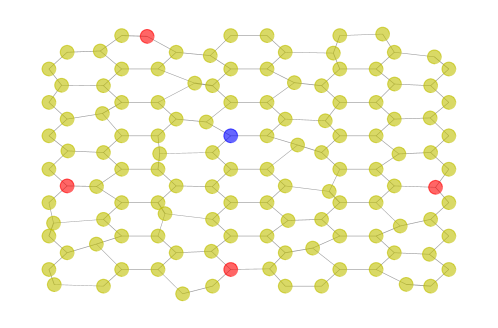
Figure 2: Example of a large graph regular graph of degree 3, where the node in blue corresponds to the oscillatory node with phase $0$ and the nodes in red correspond to the oscillatory nodes with phase $\pi$ in later simulations.

3 Results

We now show (in section 3.1) that our proposed model can find the shortest path in the cycle graph of size $5$ for a fixed source and sink, in the sense that at steady state conductivity is non-zero only on edges on the shortest path between the source and sink. We then show (in section 3.2) that this feature is maintained in simulations in the oscillatory setting when phase difference is maximised and further investigate the role of phase, amplitude and frequency. Finally, in section 3.3, we look at larger graphs with multiple oscillating nodes.

3.1 Non-oscillatory sources and sinks

Our model on $C_{5}$ (shown in Figure 1(a)) is described by the following set of equations:

$$\begin{split}\derivative{N_{1}(t)}{t}&=a+\frac{(N_{2}-N_{1})}{l_{12}}D_{12}+\frac{(N_{5}-N_{1})}{l_{51}}D_{51}\\ \derivative{N_{2}(t)}{t}&=\frac{(N_{1}-N_{2})}{l_{12}}D_{12}+\frac{(N_{3}-N_{2})}{l_{23}}D_{23}\\ \derivative{N_{3}(t)}{t}&=-bN_{3}+\frac{(N_{2}-N_{3})}{l_{23}}D_{23}+\frac{(N_{4}-N_{3})}{l_{34}}D_{34}\\ \derivative{N_{4}(t)}{t}&=\frac{(N_{3}-N_{4})}{l_{34}}D_{34}+\frac{(N_{5}-N_{4})}{l_{45}}D_{45}\\ \derivative{N_{5}(t)}{t}&=\frac{(N_{1}-N_{5})}{l_{51}}D_{51}+\frac{(N_{4}-N_{5})}{l_{45}}D_{45}\\ \derivative{D_{12}(t)}{t}&=q\frac{\absolutevalue{N_{1}-N_{2}}}{l_{12}}D_{12}-\lambda D_{12},\\ \derivative{D_{23}(t)}{t}&=q\frac{\absolutevalue{N_{2}-N_{3}}}{l_{23}}D_{23}-\lambda D_{23},\\ \derivative{D_{34}(t)}{t}&=q\frac{\absolutevalue{N_{3}-N_{4}}}{l_{34}}D_{34}-\lambda D_{34},\\ \derivative{D_{45}(t)}{t}&=q\frac{\absolutevalue{N_{4}-N_{5}}}{l_{45}}D_{45}-\lambda D_{45},\\ \derivative{D_{51}(t)}{t}&=q\frac{\absolutevalue{N_{5}-N_{1}}}{l_{51}}D_{51}-\lambda D_{51}.\end{split}$$ (8)

By setting all equations in the system (8) to zero, we derive the equilibrium points $\mathcal{E}_{1}$ and $\mathcal{E}_{2}$:

$$\mathcal{E}_{1}=(N_{1}^{*},N_{2}^{*},N_{3}^{*},N_{4}^{*},N_{5}^{*},D_{12}^{*},D_{23}^{*},D_{34}^{*},D_{45}^{*},D_{51}^{*})=$$

$$\frac{a}{b}+\frac{\lambda l_{23}}{q}+\frac{\lambda l_{12}}{q},\frac{a}{b}+\frac{\lambda l_{23}}{q},\frac{a}{b},N_{4}^{*},N_{5}^{*},\frac{aq}{\lambda},\frac{aq}{\lambda},0,0,0),$$

$$\mathcal{E}_{2}=(N_{1}^{*},N_{2}^{*},N_{3}^{*},N_{4}^{*},N_{5}^{*},D_{12}^{*},D_{23}^{*},D_{34}^{*},D_{45}^{*},D_{51}^{*})=$$

$$(\frac{a}{b}+\frac{\lambda l_{34}}{q}+\frac{\lambda l_{45}}{q}+\frac{\lambda l_{51}}{q},N_{2}^{*},\frac{a}{b},\frac{a}{b}+\frac{\lambda l_{34}}{q},\frac{a}{b}+\frac{\lambda l_{34}}{q}+\frac{\lambda l_{45}}{q},0,0,\frac{aq}{\lambda},\frac{aq}{\lambda},\frac{aq}{\lambda}).$$

These correspond to flow on the paths 1-2-3 and 1-5-4-3, respectively. Detailed derivations are provided in Appendix A. When $l_{12}+l_{23}=l_{34}+l_{45}+l_{51}$ there is an equilibrium point

$$\mathcal{E}_{3}=(N_{1}^{*},N_{2}^{*},N_{3}^{*},N_{4}^{*},N_{5}^{*},D_{12}^{*},D_{23}^{*},D_{34}^{*},D_{45}^{*},D_{51}^{*})=$$

$$\left(\frac{a}{b}+\frac{\lambda l_{23}}{q}+\frac{\lambda l_{12}}{q},\frac{a}{b}+\frac{\lambda l_{23}}{q},\frac{a}{b},\frac{a}{b}+\frac{\lambda l_{34}}{q},\frac{a}{b}+\frac{\lambda l_{34}}{q}+\frac{\lambda l_{45}}{q},\frac{aq}{2\lambda},\frac{aq}{2\lambda},\frac{aq}{2\lambda},\frac{aq}{2\lambda},\frac{aq}{2\lambda}\right).$$

The three different combinations of steady states are shown in Figure 5.

In Figure 3 we see the temporal dynamics of our model with non-oscillatory sources and sinks on the $C_{5}$ graph, for two different values of the parameter $l_{12}$. In these simulations, we set the inflow rate $a=1$, the outflow rate $b=0.5$, the parameter of reinforcement $q=0.1$, and the decay parameter $\lambda=0.01$. In the left panel $l_{12}=10$, meaning that 1-2-3 is the shortest path between the source and the sink. Whereas in the right panel $l_{12}=30$, meaning that 1-5-4-3 is the shortest path between the source and the sink. We observe that the conductivity of the edges in the shortest path increases over time until the steady state, while the conductivity of the edges that are not in the shortest path can also increase at the beginning, but will eventually converge to $0$. For the number of particles, almost all nodes have an initial accumulating period before converging to the steady states.

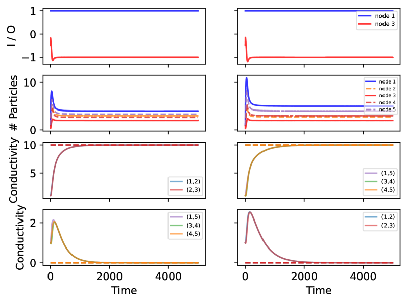
Figure 3: Results from the model on $C_{5}$ graph, with node $1$ as a source, node $3$ as a sink, an inflow at rate $a=1$, an outflow at rate $b=0.5$, and the lengths of all edges are $l_{ij}=10$ apart from $(1,2)$. On the left, we set $l_{12}=10$, thus path going through 1-2-3, is the shortest one. On the right, we set $l_{12}=30$, thus the path going through 1-5-4-3 is the shortest one. The first row shows the input at node $1$ and output at node $3$, the second row plots the number of particles on each node, $N_{i}(t)$, the third row indicates the conductivity of the edges in the shortest path, and the last row indicates the conductivity of the remaining edges in the graph, where the dashed lines in the corresponding color shows the analytical results of the steady state.

The Jacobian matrix of the system (8), is given by the following:

$$\mathbf{J}=\leavevmode\resizebox{368.57964pt}{}{$\begin{pmatrix}-\frac{D_{12}}{l_{12}}-\frac{D_{51}}{l_{51}}&\frac{D_{12}}{l_{12}}&0&0&\frac{D_{51}}{l_{51}}&\frac{N_{2}-N_{1}}{l_{12}}&0&0&0&\frac{N_{5}-N_{1}}{l_{51}}\\ \frac{D_{12}}{l_{12}}&-\frac{D_{12}}{l_{12}}-\frac{D_{23}}{l_{23}}&\frac{D_{23}}{l_{23}}&0&0&\frac{N_{2}-N_{1}}{l_{12}}&\frac{N_{3}-N_{2}}{l_{23}}&0&0&0\\ 0&\frac{D_{23}}{l_{23}}&-b-\frac{D_{23}}{l_{23}}-\frac{D_{34}}{l_{34}}&\frac{D_{34}}{l_{34}}&0&0&\frac{N_{3}-N_{2}}{l_{23}}&\frac{N_{4}-N_{3}}{l_{34}}&0&0\\ 0&0&\frac{D_{34}}{l_{34}}&-\frac{D_{34}}{l_{34}}-\frac{D_{45}}{l_{45}}&\frac{D_{45}}{l_{45}}&0&0&\frac{N_{3}-N_{4}}{l_{34}}&\frac{N_{5}-N_{4}}{l_{45}}&0\\ \frac{D_{51}}{l_{51}}&0&0&\frac{D_{45}}{l_{45}}&-\frac{D_{45}}{l_{45}}-\frac{D_{51}}{l_{51}}&0&0&0&\frac{N_{4}-N_{5}}{l_{45}}&\frac{N_{1}-N_{5}}{l_{51}}\\ \frac{q\operatorname{sgn}{(N_{1}-N_{2})}D_{12}}{l_{12}}&\frac{q\operatorname{sgn}{(N_{1}-N_{2})}D_{12}}{l_{12}}&0&0&0&\frac{q|N_{1}-N_{2}|}{l_{12}}-\lambda&0&0&0&0\\ 0&\frac{q\operatorname{sgn}{(N_{2}-N_{3})}D_{23}}{l_{23}}&\frac{q\operatorname{sgn}{(N_{2}-N_{3})}D_{23}}{l_{23}}&0&0&0&\frac{q|N_{2}-N_{3}|}{l_{23}}-\lambda&0&0&0\\ 0&0&\frac{q\operatorname{sgn}{(N_{3}-N_{4})}D_{34}}{l_{34}}&\frac{q\operatorname{sgn}{(N_{3}-N_{4})}D_{34}}{l_{34}}&0&0&0&\frac{q|N_{3}-N_{4}|}{l_{34}}-\lambda&0&0\\ 0&0&0&\frac{q\operatorname{sgn}{(N_{4}-N_{5})}D_{45}}{l_{45}}&\frac{q\operatorname{sgn}{(N_{4}-N_{5})}D_{45}}{l_{45}}&0&0&0&\frac{q|N_{4}-N_{5}|}{l_{45}}-\lambda&0\\ \frac{q\operatorname{sgn}{(N_{5}-N_{1})}D_{51}}{l_{51}}&0&0&0&\frac{q\operatorname{sgn}{(N_{5}-N_{1})}D_{51}}{l_{51}}&0&0&0&0&\frac{q|N_{5}-N_{1}|}{l_{51}}-\lambda\end{pmatrix}$}$$ (9)

In the appendix A, we show that for all three steady states, this Jacobian matrix will have zero determinant, meaning that at least one eigenvalue of the Jacobian matrix will be 0. Thus, the steady states will be non-hyperbolic, implying that studying the eigenvalues of the Jacobian is not enough to determine stability of the steady states. A full analysis of the steady states using center manifold theory would be required to do this [56].

Nonetheless, we can use the Jacobian matrix to understand more about what happens to the system. We note that when $D_{12}^{*}=D_{23}^{*}=0$ or $D_{34}^{*}=D_{45}^{*}=D_{51}^{*}=0$, at least one row in the Jacobian matrix will contain only zero values, and thus span a slow manifold. For the Jacobian matrix evaluated at $\mathcal{E}_{1}$, the eigenvectors corresponding to the zero eigenvalues will be $(0,0,0,1,0,0,0,0,0,0)$ and $(0,0,0,0,1,0,0,0,0,0)$. The implication of this observation is that there is a line of steady states for both $N_{4}^{*}$ and $N_{5}^{*}$, which form the slow manifold. For the Jacobian matrix evaluated at $\mathcal{E}_{2}$, the eigenvector corresponding to the zero eigenvalue will be $(0,1,0,0,0,0,0,0,0,0)$, corresponding to a line of steady states for $N_{2}^{*}$ which also is a slow manifold. These slow manifolds corresponds to the nodes with no edges, meaning that there are particles left behind at these edges, that are stuck because the conductivity converges to 0 for the longer paths.

The numerical bifurcation diagram in Figure 4 looks at the role of $l_{12}$ as a bifurcation parameter. In Figure 4 (a) we see that the number of particles at node 3, $N_{3}^{*}$ is always $a/b$, independent on the length $l_{12}$. However, $N_{1}^{*}$, $N_{4}^{*}$ and $N_{5}^{*}$, increase linearly as $l_{12}$ approaches the equilibrium point 20, after which they all are constant. $N_{2}^{*}$ is constant ($\frac{a}{b}+\frac{\lambda l_{23}}{q}=3$) until the bifurcation point $l_{12}=20$, where it instead decrease linearly. In Figure 4 (b) we see that the conductivity of edges on the shortest path is always $aq/\lambda$, and 0 for the edges that are not the shortest path. When the length of $l_{12}$ approaches the bifurcation point 20, the simulations has not reached steady state after 100000 time steps, and is thus not 0 and $aq/\lambda$ in the plot. When $l_{12}=20$ the two paths are of equal lengths and $D_{ij}=\frac{aq}{2\lambda}$ for all $(i,j)$.

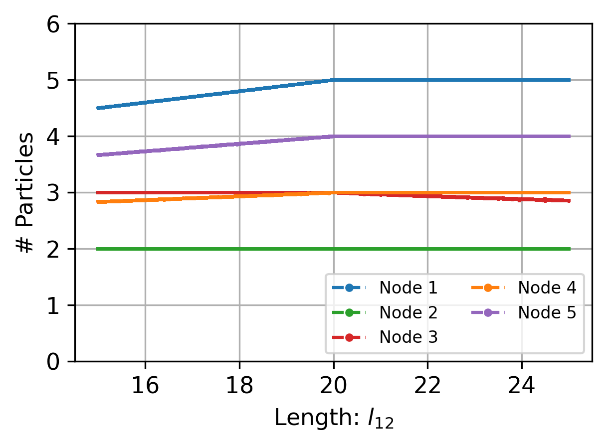
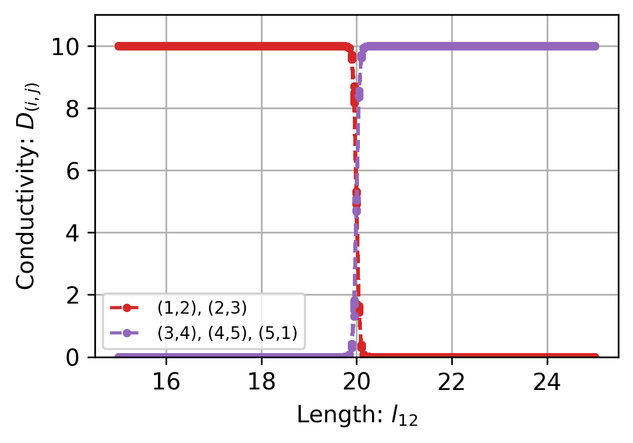
Figure 4: Bifurcation diagram with $l_{12}$ as bifurcation parameter. Here $l_{23}=l_{34}=l_{45}=l_{51}=10$, $a=1.0$, $b=0.5$, $q=0.1$ and $\lambda=0.01$. The diagram is generated by simulating the equation system (10) through 100,000 time steps, each time initiated with random initial conditions. This process is repeated 10 times for each $l_{12}$ value, with the bifurcation diagram displaying the results from the last 100 time steps of each simulation.

Figure 5 illustrates the overall picture. In (a) we see that when 1-2-3 is the shortest path, there is a non-hyperbolic equilibrium where the conductivity on the edges of the longest path is zero, but the conductivity of the edges of the shortest path is $\frac{aq}{\lambda}$. The number of particles at the nodes with no connections, $N_{4}^{*}$ and $N_{5}^{*}$, spans the slow manifold. In (b) the paths 1-2-3 and 3-4-5-1 are of equal lengths and the conductivity of all edges is $\frac{aq}{2\lambda}$. When the path through nodes 1-2-3 is longer than 1-5-4-3 (Figure 5 (c)), the non-hyperbolic equilibrium point corresponds to having zero-conductivity on the edges going through node 2, and a line of steady states for the number of particles on node 2, $N_{2}^{*}$. The conductivity on the edges on the shortest path is $\frac{aq}{\lambda}$.

(a) Non-hyperbolic stable equilibrium when $l_{12}+l_{23}<l_{34}+l_{45}+l_{51}$ ($\mathcal{E}_{1}$).

(b) Non-hyperbolic stable equilibrium when $l_{12}+l_{23}=l_{34}+l_{45}+l_{51}$ ($\mathcal{E}_{3}$).

(c) Non-hyperbolic stable equilibrium when $l_{12}+l_{23}>l_{34}+l_{45}+l_{51}$ ($\mathcal{E}_{2}$).

Figure 5: Different equilibrium points for the model on the $C_{5}$ with non-oscillatory sources and sinks, where node 1 (blue) is a source, and node 3 (red) is a sink. In (a) we see the stable equilibrium when 1-2-3 is the shortest path, in (b) we see the stable equilibrium when both paths have equal length, and in (c) we see the stable equilibrium when 1-5-4-3 is the shortest path.

3.2 Oscillatory nodes

We now use simulations to explore the behaviour of the model with oscillatory nodes on a $C_{5}$ graph. We start from the case when the two oscillatory nodes have phase difference $\pi$ (i.e. completely out of phase) and then explore the behaviour of the model when we vary the phase difference between $-\pi$ and $\pi$. Finally, we look at how the amplitude and frequency of the oscillatory nodes affect the model. Throughout the section, we set nodes $1$ and $3$ to be the oscillatory nodes, and the length of all edges to be $l_{ij}=10$, thus the shortest path between the two oscillatory nodes is known to be $e_{1}e_{2}$ where $e_{1}=(1,2)$ and $e_{2}=(2,3)$.

Phase difference. Figure 6 shows the temporal dynamics of our model when the two oscillatory nodes have phase difference $\pi$. The top two panels of the figure show the oscillating input and outputs over two different time windows. The number of particles at node 1 and 3 have the same frequency as the inputs and outputs, but with a short delay as the particles flow into and out of the nodes. Oscillations with similar frequency can be seen at nodes 4 and 5, which are on the longer path, but with much smaller amplitude and a different phase. Node 2, which is on the shortest path, reaches steady state.

The conductivity of edges oscillates over time, but they also change over a longer time scale. Specifically, the median conductivity of the edges on the shortest path generally increases, but with a rate of increase that tends very slowly towards $0$. Interestingly, the number of particles oscillates at a frequency that is almost half that of the conductivity on the edges. This is presumably because the flow shuttles backwards and forwards. Moreover, the amplitude of the conductivity changes is much smaller than that of the oscillations of particles at nodes 1 and 3 (note the scale on the axis for conductivity in Figure 6). The median conductivity of the edges that are not on the shortest path decrease over time and converge to values either $0$ or very close to $0$ (with no or very small oscillations) depending on the initial conditions (see the bottom row of Figure 6).

We observe similar features of the model on cycles of larger sizes and also graphs of more general structure (see more details in Appendix B.2).

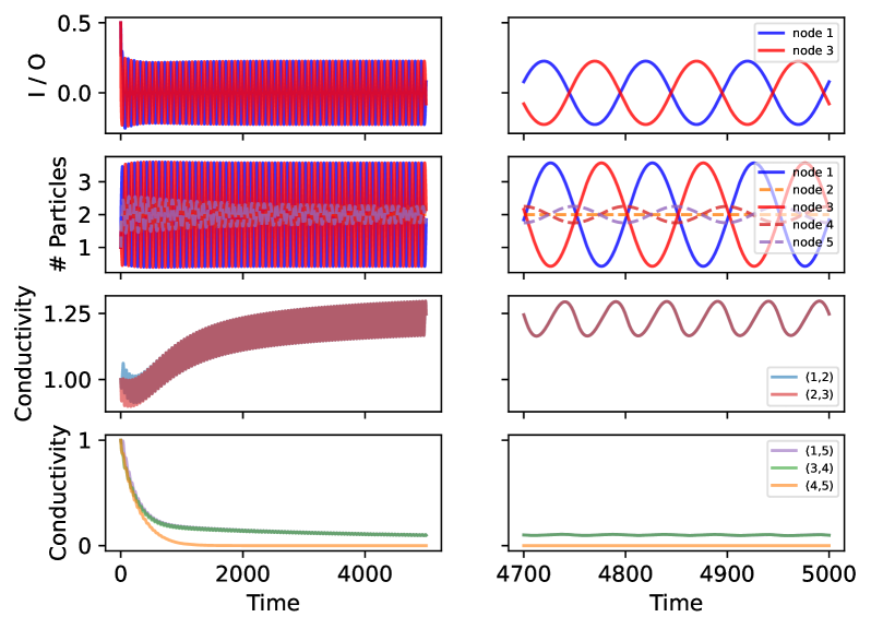
Figure 6: Results from the model on a $C_{5}$ graph, with nodes 1 and 3 as the oscillating nodes, rate $b=0.5$, amplitude $A_{1}=A_{3}=A=1$, frequency $\theta_{1}=\theta_{3}=\theta=0.01$, and phases $\phi_{1}=0$ and $\phi_{3}=\pi$, with the same reinforcement parameter $q=0.1$ and decay parameter $\lambda=0.01$ as in Figure 3. The first row plots the actual input/output to the two nodes, the second row shows the number of particles in each node, the third row indicates the conductivity of the edges in the shortest path and the last row indicates the conductivity of the remaining edges in the graph, with the full profile on the left while the change in the long term on the right.

In Figure 7 we examine the change of conductivity over the change of phase difference $\phi_{3}-\phi_{1}$, from $-\pi$ to $\pi$. When the phase difference is $-\pi$, the conductivity of edges on the shortest path is maximal (see the points corresponding to phase difference $-\pi$ at the left most of Figure 7). As the phase difference becomes closer to one, the conductivity of the edges on the shortest path decreases, with that of the edge $(2,3)$ approaching $0$. Correspondingly, the conductivity of edges $(3,4)$ and $(1,5)$ slowly increases. In this situation, the two oscillating nodes are connected via the shortest paths, but have additional arms that reach out along the longer path but do not connect.

For phase differences between around $-0.65\pi$ and $0$ the network becomes disconnected: the conductivity of edges does not change with phase and is zero for the edge $(1,2)$ (see the corresponding region in Figure 7). When the phase difference is $0$, the two edges on the shortest path have the same conductivity value, as do the other two disconnected arms on the longer path. As the phase difference increases from $0$ up until around $0.65\pi$, the conductivity of edges stabilises again with $(2,3)$ now having zero conductivity. The same pattern is repeated now in the sense that the results are invariant if we change the label of node $1$ with $3$, and that of nodes $4$ and $5$.

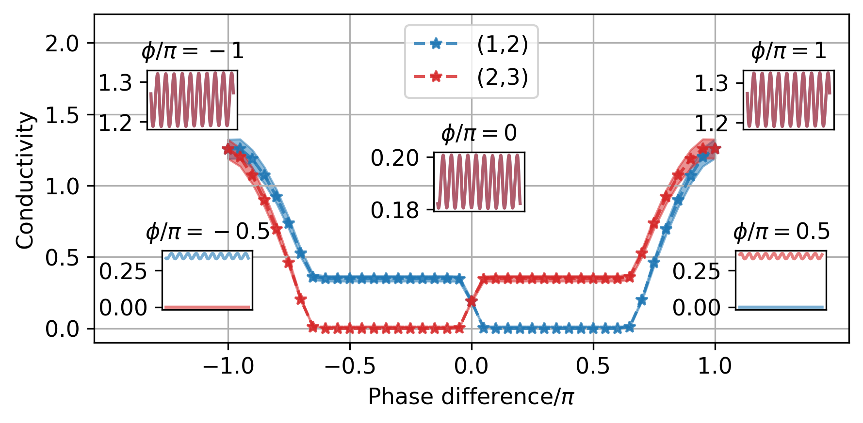
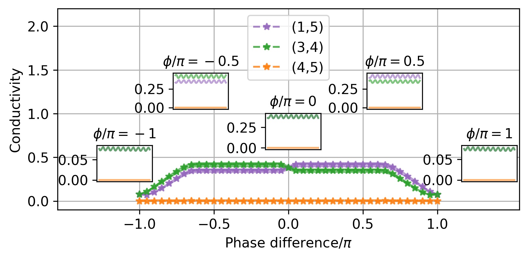
Figure 7: Conductivity results from the model on a $C_{5}$ graph, from edges in the shortest path (top) and not (bottom) after sufficiently long time (where the oscillation repeats) subject to changing phase difference between the two oscillatory nodes $3$ and $1$, where other parameters are the same as in Figure 6, the line with asterisk markers indicate the middle value, and the shade indicates the amplitude. The inserted subfigures indicate the change of conductivity of edges along time in sufficiently long time.

Amplitude, frequency and phase differences. When the amplitude or the frequency of the two oscillatory nodes are not exactly the same, the model exhibits a rich span of behaviours. In Figure 8, we explore the resulting graphs as we change both phase difference $\Delta\phi=\phi_{3}-\phi_{1}$ and amplitude ratio $A_{3}/A_{1}$. In these figures, the thickness of the edges indicates their conductivity after the simulation has been run sufficiently long time. The middle row where $A_{3}/A_{1}=1$ corresponds to the case presented in Figure 7, and discussed in detail in the last paragraph, where the graph changes from at first being connected via the shortest path ($\Delta\phi=-3\pi/4$) and having additional arms, to becoming disconnected (e.g. $\Delta\phi=-\pi/4$), to connecting again ($\Delta\phi=3\pi/4$) and the majority of the flow following the shortest path ($\Delta\phi=\pi$).

When $A_{3}/A_{1}$ is close to $1$, the results exhibit similar phase transitions to the case of $A_{3}/A_{1}=1$; see the rows corresponding to $\Delta\phi=9/10,10/9$ in Figure 8. As the amplitude ratio $A_{3}/A_{1}$ increases, edges generally have larger values of conductivity. For example, when $A_{3}/A_{1}=2$, all edges have nonzero conductivity values for all possible values of the phase difference $\Delta\phi$. Moreover, if $\Delta\phi$ is close to $-\pi$ or $\pi$, the edges in the shortest path have higher conductivity values than others. When $A_{3}/A_{1}=3$ (and for larger values) the edges on the shortest path always have higher conductivity values than others, independent of $\Delta\phi$. Amplitude differences can thus lead to a greater concentration of flow on the shorter path.

When the amplitude ratio $A_{3}/A_{1}$ is smaller than one, edges generally have smaller values of conductivity. Specifically, when $A_{3}/A_{1}=1/2$ there are no edges that are incident on oscillatory node $3$ with non-zero conductivity values when the phase difference $\Delta\phi\leq 0$. There is also only a weak connection between oscillatory node $3$ and node $2$ in the shortest path when $\Delta\phi>0$. When $A_{3}/A_{1}$ is $1/5$ or $1/10$, this disconnected network is the outcome for all possible values of $\Delta\phi$.

$A_{3}/A_{1}\backslash\Delta\phi$	$-\frac{3\pi}{4}$	$-\frac{\pi}{2}$	$-\frac{\pi}{4}$	$0$	$\frac{\pi}{4}$	$\frac{\pi}{2}$	$\frac{3\pi}{4}$	$\pi$
$1/10$
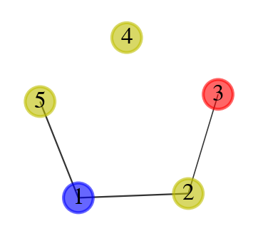
$1/3$
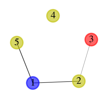
$1/2$
$4/5$
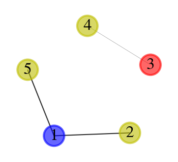
$9/10$
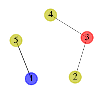
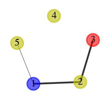
$1$
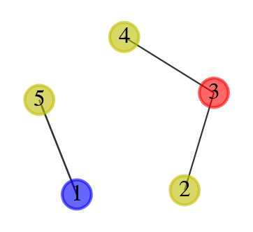
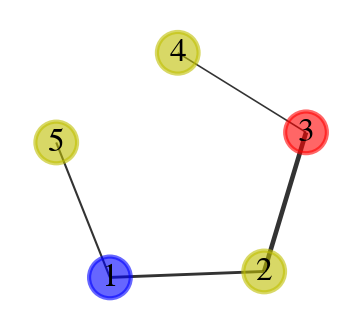
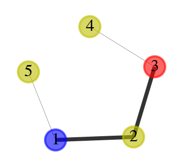
$10/9$
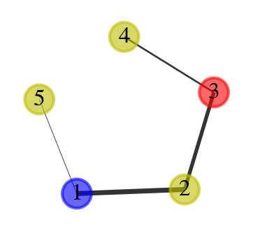
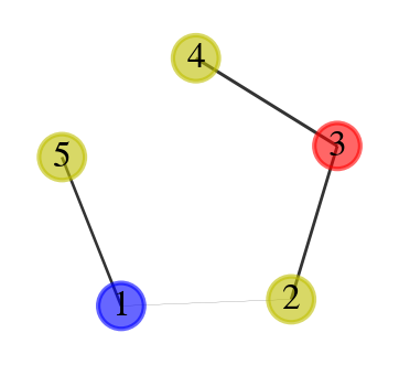
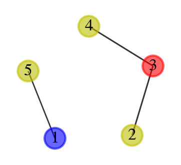
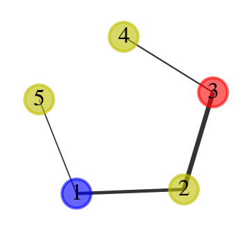
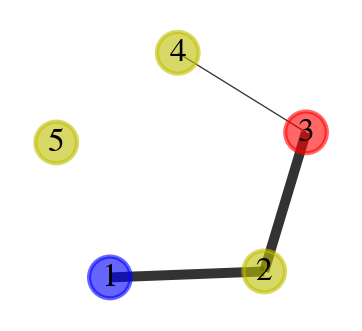
$5/4$
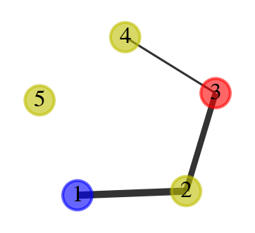
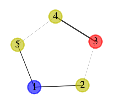
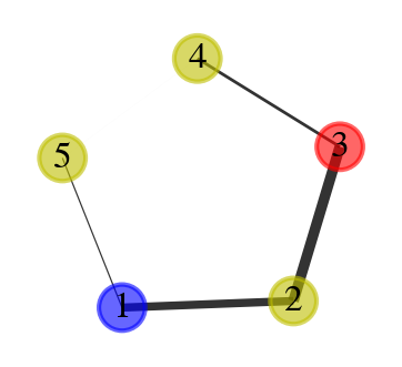
$2$
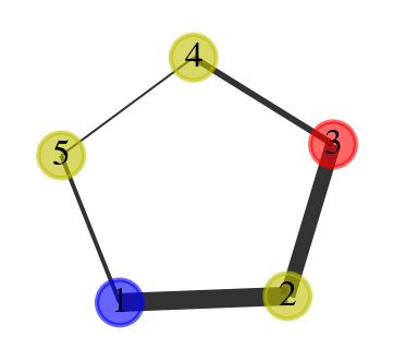
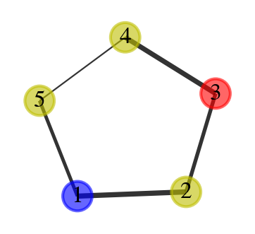
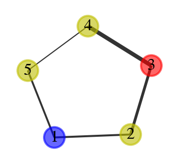
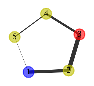
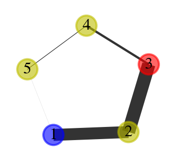
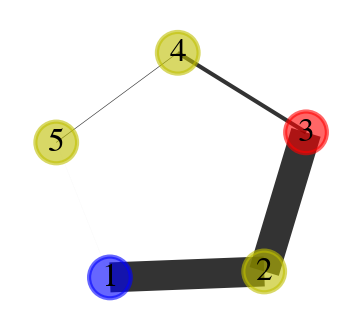
$3$

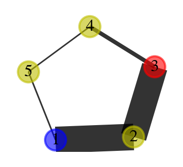
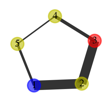
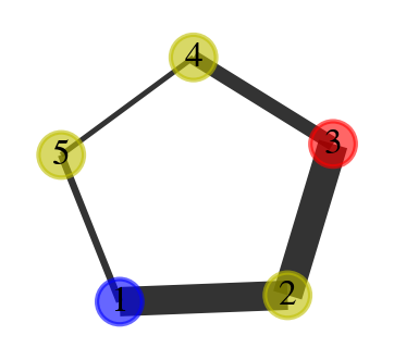
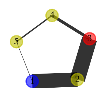
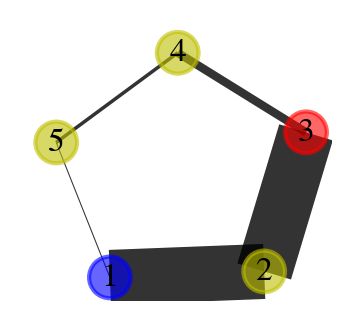
Figure 8: Conductivity results (median) from the model on a $C_{5}$ graph at long enough time, subject to changing amplitude ratio $\alpha=A_{3}/A_{1}$ ($A_{1}=1$) and phase difference $\Delta\phi=\phi_{3}-\phi_{1}$ ($\phi_{1}=0$), where other parameters are the same as in Figure 6, and the thickness of edges is proportional to the conductivity value.

In Figure 9, we examine the resulting graphs as we change both phase difference $\Delta\phi=\phi_{3}-\phi_{1}$ and frequency ratio $\theta_{3}/\theta_{1}$. In these figures, the thickness of the edges, again, indicates their conductivity after the simulation has been run sufficiently long time. The third row where $\theta_{3}/\theta_{1}=1$ corresponds to the case presented in Figure 8, exhibiting different features as the phase difference changes, as in the case of $A_{3}/A_{1}=1$ in the last paragraph.

However, when the frequency ratio $\theta_{3}/\theta_{1}\neq 1$, the resulting graphs remain the same at all phase difference values. As the frequency ratio $\theta_{3}/\theta_{1}$ increases, less edges have nonzero conductivity in general. For example, when $\theta_{3}/\theta_{1}=2$ or $5$, only edges that are incident on either of the two oscillatory nodes have nonzero conductivity values. When $\theta_{3}/\theta_{1}=7$, the edge that is incident on oscillatory node $3$ but not in the shortest path now has zero conductivity. In these two cases, the two oscillatory nodes are then connected via the shortest path and have additional arm(s). When $\theta_{3}/\theta_{1}=10$, no edges that are incident on oscillatory node $3$ have nonzero conductivity, thus the graph become disconnected. Hence, frequency can affect the exploration depth of the flow on the graph.

As the frequency ratio $\theta_{3}/\theta_{1}$ decreases, more edges have nonzero conductivity on the whole. Specifically, when $\theta_{3}/\theta_{1}=1/2$, all edges apart from the one that is not incident on either of the oscillatory nodes have zero conductivity. When $\theta_{3}/\theta_{1}=1/10$, all edges now have nonzero conductivity values, even though the conductivity of the one that has zero conductivity in the previous case is very small.

With all above, we conclude that amplitude, frequency and phase all contain important information for the model to learn interesting patterns in the graph and the change in the environment.

$\theta_{3}/\theta_{1}\backslash\Delta\phi$	$-\frac{3\pi}{4}$	$-\frac{\pi}{2}$	$-\frac{\pi}{4}$	$0$	$\frac{\pi}{4}$	$\frac{\pi}{2}$	$\frac{3\pi}{4}$	$\pi$
$1/10$
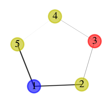
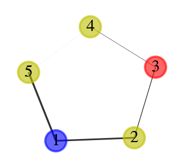
$1/2$
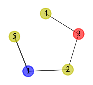
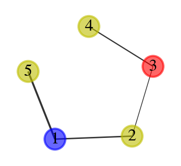
$1$
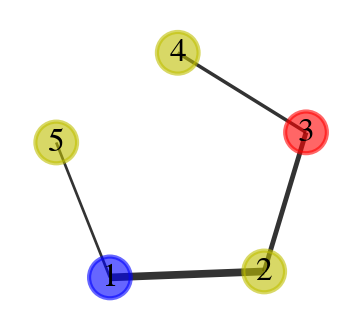
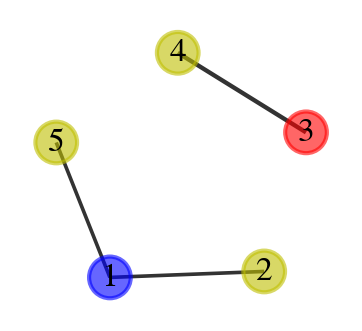
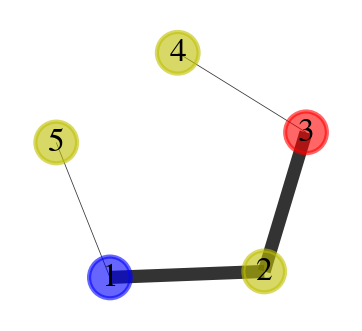
$2$
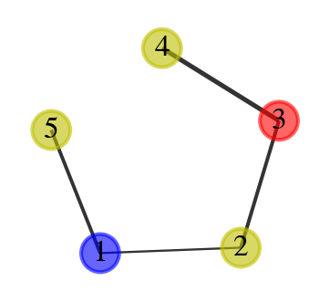
$5$
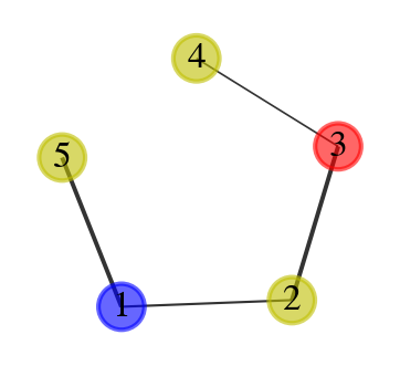
$7$
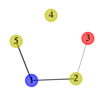
$10$

Figure 9: Conductivity results (median) from the model on a $C_{5}$ graph at long enough time, subject to changing frequency ratio $\gamma=\theta_{3}/\theta_{1}$ ($\theta_{1}=0.01$) and phase difference $\Delta\phi=\phi_{3}-\phi_{1}$ ($\phi_{1}=0$), where other parameters are the same as in Fig. 6, and the thickness of edges is proportional to the conductivity value.

3.3 Large graphs

We now proceed to examine the behaviour of the model, with oscillatory nodes, on larger graphs (see section 2.5 for the setup). The purpose of this investigation was to see if the model could also produce large-scale patterns with shortest path connections between the nodes in the presence of external oscillations.

In Figure 10, we explore the behaviour of our model after sufficiently long time in two different cases: where there are three oscillatory nodes (the blue node in Figure 2 and the two red nodes horizontally in the middle of the figure) and where five oscillatory nodes (one blue and four red) are included. In both these simulations, the flow is still focused primarily on the shortest paths between the oscillatory nodes with the largest phase differences (black connecting lines in Figure 10). The oscillations dominate the behaviour of the particles. Following Figure 10a to 10b to 10c we see that the concentration of particles goes from the periphery to the centre and then out to the periphary again. Figure 10d to 10e to 10f shows the same pattern but for five nodes.

While identifying parameter values to produce this outcome, we noted that frequency of oscillatory nodes is more important in large graphs than the smaller examples we have already seen. The oscillations should be sufficiently slow to allow the information from one oscillatory node to communicate with another, before the particles go back along the paths they have travelled from. Meanwhile, the amplitude should be sufficiently large to allow such communication before the conductivity reduces to $0$. Hence in the simulations on larger graphs, we set the frequency to be $\theta=0.001$ and amplitude to be $A=5$, while maintaining the parameter of reinforcement being $q=0.1$ and the decay parameter $\lambda=0.01$.

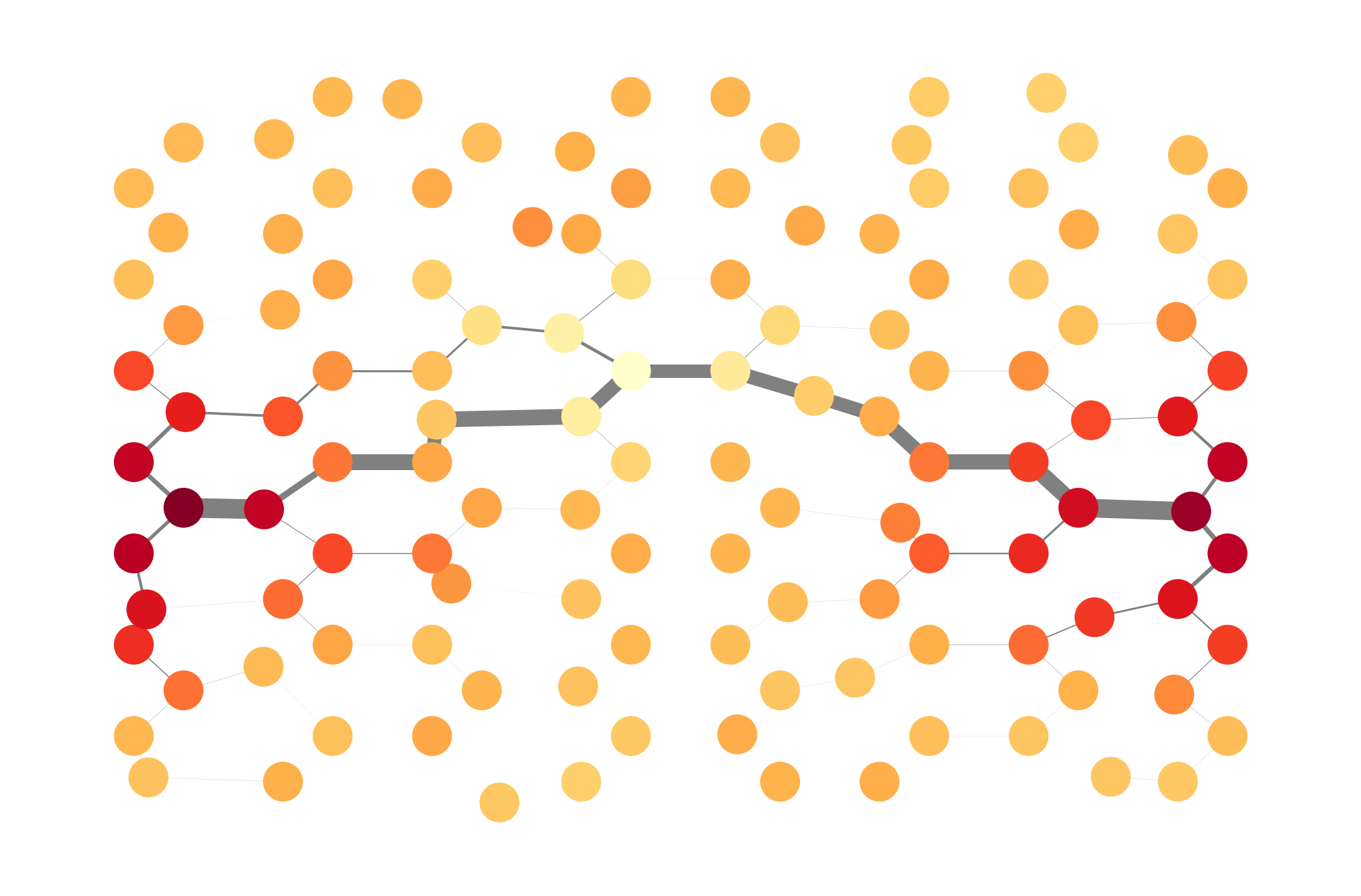
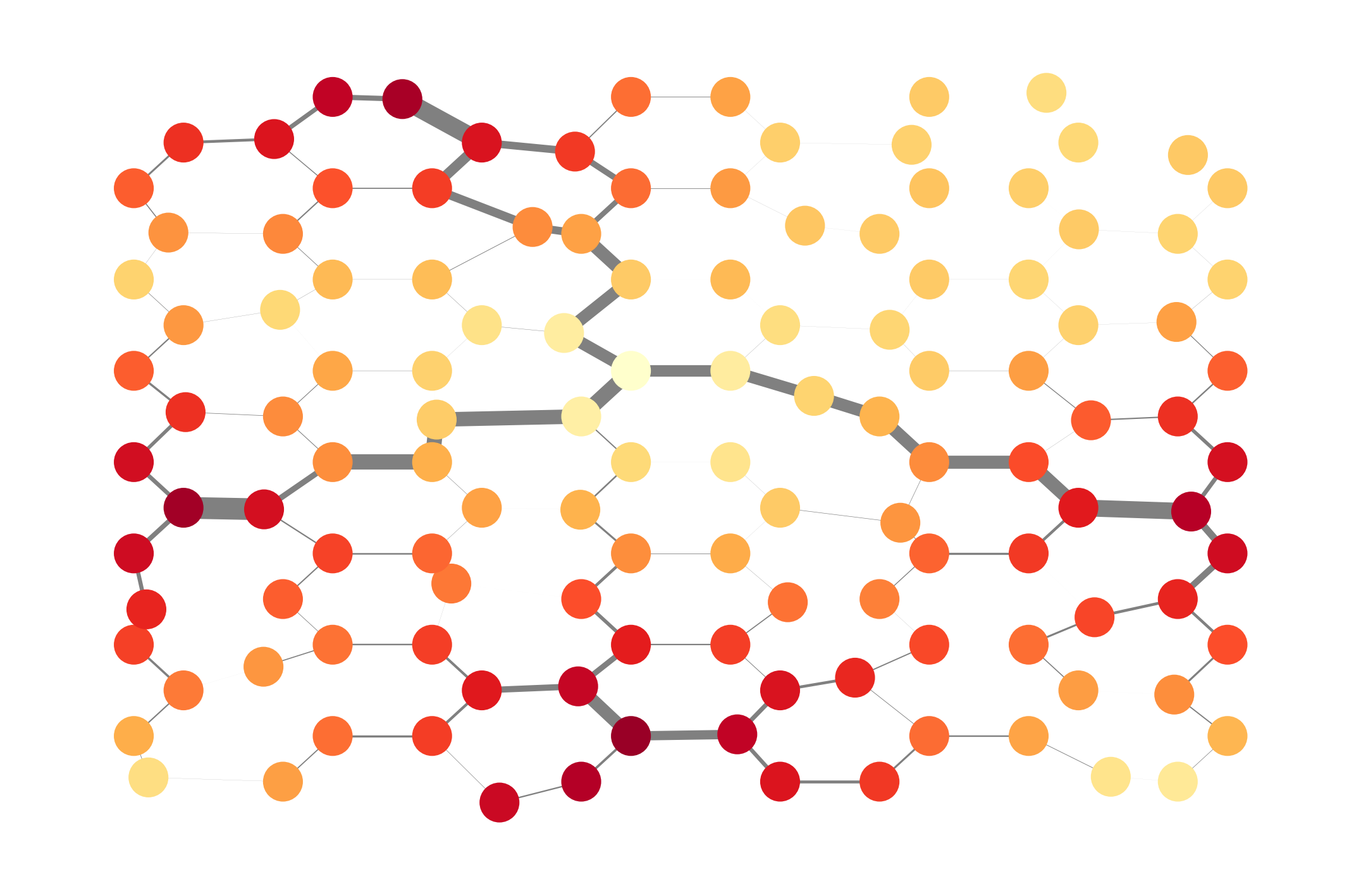
(a)	(d)
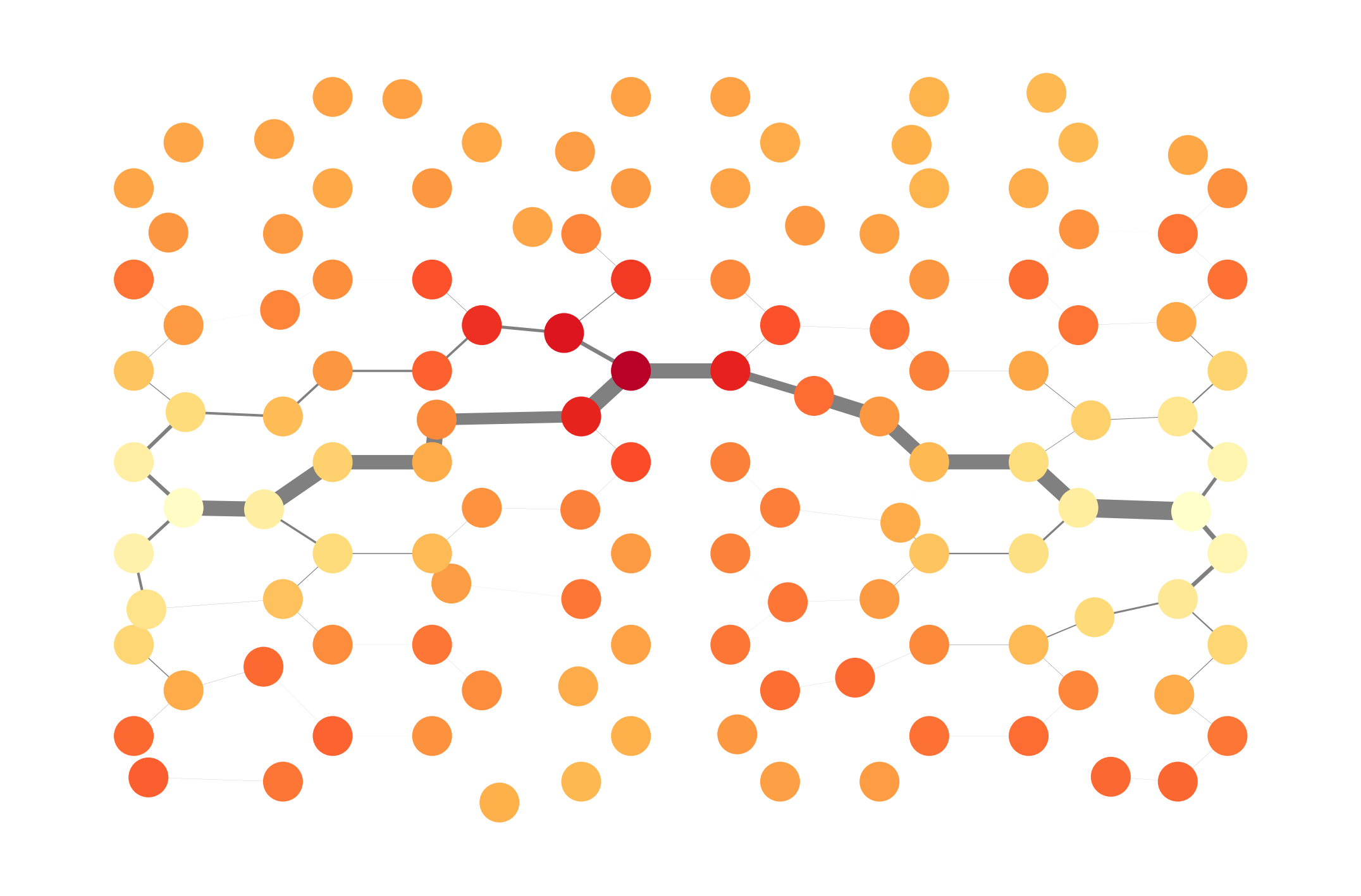
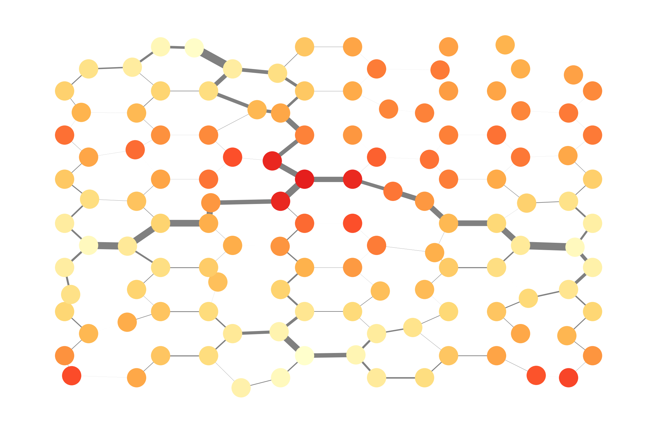
(b)	(e)
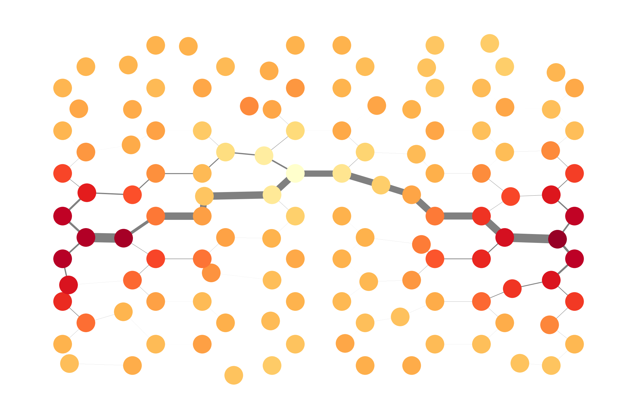
(c)	(f)

Figure 10: Snapshots of the graphs at three different representative time points in sufficiently long time, with various number of oscillatory nodes. (a),(b),(c): $3$ oscillatory nodes, with equal time difference. (d),(e),(f): $5$ oscillatory nodes, with equal time difference. The edge thickness in the graphs is proportional to the conductivity, and the node redness is proportional to the number of particles.

4 Discussion

Guided by Beer’s four steps [33, 38], we have provided and investigated a mathematical framework inspired by organisms exhibiting basal cognition [13]. Under this framework, the formulation of the model is itself a contribution to this research area: we have built upon previous models of current reinforcement to explicitly include oscillations, demonstrating that such systems often exhibit the greatest flow on the shortest path between the oscillators.

We can think of our model as a demonstration of how organisms can monitor a dynamic environment, transporting particles (e.g. nutrients or signals) effectively between different locations. These abilities existed well before the development of nervous systems, let alone central nervous systems [13]. This makes our model a potential step towards a more realistic slime mould model [31], as it captures both synchronisation and network construction observed in experiments of these organisms [23, 42]. It also mimics other types of basal cognition, such as macromolecular networks in microbes [40], and signalling in fungi [39].

In a stationary environment the current or flow of particles converges to an efficient transport network on the shortest path. Previous work on current reinforced models has proven that a shortest path is established in a model where the flow of particles is assumed to be at steady state [43, 44]. We have found that if we explicitly model the dynamics of that flow then, while flow is still concentrated on the shortest path, there exist non-hyperbolic stable node configurations. These correspond to particles which, might be said to be, ‘stuck’ on the longer path. We suggest a connection between these stuck particles and the way in which many organisms with basal cognition have an external memory. By leaving external cues in the environment, they can react when the environment changes [57]. We have established that the stuck particles are associated with a slow manifold. This means we have very slowly changing particle numbers on the longer path spanning the slow manifold, while flow on the network converges to the shortest path. In this way, the model has an external memory: the particles on the nodes corresponding to the longer path ‘remember’ failed solutions, and might be reactivated when conditions change.

The dynamic networks in our simulations produce both efficient flow and long-range oscillatory dynamics. While the nodes oscillate greatly in terms of number of particles at them, the connecting edges of the graph experience only small oscillations (this can be seen by contrasting the scale of the oscillations in conductivity and number of particles in Fig. 6). The resulting pattern has low frequency responses to changes in formation over a long range combined with a rapid flow of information across the system. We see this in Figure 10, which is reminiscent of cross-frequency coupling, i.e. coupling between neurons of different frequency, which has been proposed as a mechanism for working memory [6, 7]. This is in contrast to the Kuramoto model, which captures synchronisation, but does not capture information transfer in the same way as our model.

Comparing our model to recent slime mould models created by Alim et al. [53], our analysis reveals that reinforcement coupled with oscillators can indeed find the shortest path, as suggested by these authors, and similar to what is found by Watanabe et al. [45]. However, in contrast to Watanabe et al., the sum of the input and output rates in our model are not set to zero. Yet, after reaching a stable limit cycle, the input and output rates in our model cancel out, suggesting that the oscillators self-organize to have the total flux to/from the system balanced. Our work also aligns with Reid’s perspective on slime mold as a connected mass of oscillating units [58]. It further echoes early experiments by Takamatsu et al., displaying similar oscillatory behavior in conductivity (i.e. thickness of the plasmodium network) in rings of slime mould oscillators [29, 30].

Expanding our discussion to other species with basal cognition, we can draw parallels between our model and experiments in bacterial colonies that employ in phase and anti-phase oscillatory behaviors during resource scarcity[35]. Similarly, the in-phase and out-of-phase oscillatory behaviour in our model are akin to the emergence of in-phase and out-of-phase oscillatory behaviour that is also found in plant shoots. For example, emergent maize plants grow in a group which exhibit synchronized oscillatory motions that may be in-phase or anti-phase [59]. Drawing connections to fungal mycelia, our model resonates with recent studies highlighting the bidirectional transport of signals and nutrients [39]. The flexibility of nodes to switch between acting as sources and sinks in our model provides a promising foundation for modeling bidirectional transportation within fungal mycelia [39].

Our analysis shows that not only phase, but also amplitude and frequency of oscillations can induce the construction of efficient transport networks. This confirms (in a model) the hypothesis of Boussard et al. (2021), who suggested that all three variations could play a role in how slime moulds build networks [14]. Phase differences certainly play a relatively more important role, especially when the oscillatory nodes are close to being out-of-phase. In this case, the model nearly always has almost all its flow on the shortest path between the out pf phase nodes. But variations in any one, or a combination of phase, amplitude and frequency are sufficient to produce the basal cognition we observe in our simulations.

We do observe that very big frequency differences inhibits shortest path formation. For example, the oscillating nodes become disconnected when the frequency ratio is 10 (see bottom row of Figure 9). This, along with the need for the oscillators to be (somewhat) out of phase, gives some restrictions on the types of oscillations needed in order to create a flow between nodes. Amplitude primarily effects how far the particles can explore in the graph: too small amplitudes do not allow long range communication.

Our model does not include feedback between oscillatory nodes, which we know are part of how living organisms assess, engage and adapt to the world around them. Such feedback could also potentially change the phase, amplitude and frequency of the oscillations towards values which better facilitate communications. Our next modelling steps would therefore be to incorporate feedback mechanisms for the oscillators into the model (as suggested by [14]). The introduction of feedback could involve the consideration of diverse forms of local information, $lc_{i}(t)$, such as the potential difference in particles ($\sum_{j\in\Gamma(i)}(N_{i}(t)-N_{j}(t))$), the absolute potential difference, or a combination of potential difference and conductivity ($\sum_{j\in\Gamma(i)}(N_{i}(t)-N_{j}(t))D_{ij}(t)$). Moreover, an exploration could encompass various strategies for the phase transition, including the option of direct proportionality to local information ($\frac{d\phi_{i}(t)}{dt}=lc_{i}(t)$). An initial exploration using smaller networks could be undertaken to discern the impact of network topology on feedback forms, as done by Ma et al. [60]. Alternatively, an evolutionary adaptive approach, as advocated by Beer [38], offers another way to learn a feedback scheme.

In conclusion, the model we propose here already has similar properties to many biological systems which exhibit basal (or even more complex forms of) cognition. We see it as a promising starting point for future simulation models of these phenomena.

Appendix A Non-oscillatory sources and sinks

A.1 Steady states

This section of the appendix derives the results for the steady states as presented in Section 3.1. The equilibrium points of the system are determined by the solutions to the following set of equations:

$$a+\frac{(N_{2}^{*}-N_{1}^{*})}{l_{12}}D_{12}^{*}+\frac{(N_{5}^{*}-N_{1}^{*})}{l_{51}}D_{51}=0,$$ (10)

$$\frac{(N_{1}^{*}-N_{2}^{*})}{l_{12}}D_{12}^{*}+\frac{(N_{3}^{*}-N_{2}^{*})}{l_{23}}D_{23}^{*}=0,$$ (11)

$$-bN_{3}^{*}+\frac{(N_{2}^{*}-N_{3}^{*})}{l_{23}}D_{23}^{*}+\frac{(N_{4}^{*}-N_{3}^{*})}{l_{34}}D_{34}^{*}=0,$$ (12)

$$\frac{(N_{3}^{*}-N_{4}^{*})}{l_{34}}D_{34}^{*}+\frac{(N_{5}^{*}-N_{4}^{*})}{l_{45}}D_{45}^{*}=0,$$ (13)

$$\frac{(N_{1}^{*}-N_{5}^{*})}{l_{51}}D_{51}^{*}+\frac{(N_{4}^{*}-N_{5}^{*})}{l_{45}}D_{45}^{*}=0,$$ (14)

$$q\frac{\absolutevalue{N_{1}^{*}-N_{2}^{*}}}{l_{12}}D_{12}^{*}-\lambda D_{12}^{*}=0,$$ (15)

$$q\frac{\absolutevalue{N_{2}^{*}-N_{3}^{*}}}{l_{23}}D_{23}^{*}-\lambda D_{23}^{*}=0,$$ (16)

$$q\frac{\absolutevalue{N_{3}^{*}-N_{4}^{*}}}{l_{34}}D_{34}^{*}-\lambda D_{34}^{*}=0,$$ (17)

$$q\frac{\absolutevalue{N_{4}^{*}-N_{5}^{*}}}{l_{45}}D_{45}^{*}-\lambda D_{45}^{*}=0,$$ (18)

$$q\frac{\absolutevalue{N_{5}^{*}-N_{1}^{*}}}{l_{51}}D_{51}^{*}-\lambda D_{51}^{*}=0.$$ (19)

In general, the steady states for the conductivity are given by the equation:

$$q\frac{\absolutevalue{N_{i}^{*}-N_{j}^{*}}}{l_{ij}}D_{ij}^{*}-\lambda D_{ij}^{*}=0.$$ (20)

For this to hold, either $D_{ij}^{*}=0$ or $\absolutevalue{N_{i}^{*}-N_{j}^{*}}=\frac{\lambda l_{ij}}{q}$. If $D_{ij}^{*}\neq 0$, then $\absolutevalue{N_{i}^{*}-N_{j}^{*}}=\frac{\lambda l_{ij}}{q}$, and thus, Equation (20) can be simplified to

$$\pm\frac{\lambda}{q}D_{{i-1},i}^{*}+\pm\frac{\lambda}{q}D_{i,{i+1}}^{*}=0.$$ (21)

As $D_{ij}(t)$ denotes the conductivity, we know that $D_{ij}(t)\geq 0$ and thus, the two addends must have opposite signs. This gives the solution

$$D_{{i-1},i}^{*}=D_{i,{i+1}}^{*}.$$ (22)

This also implies that for a node $i$, which is neither a source nor a sink, $(N_{i-1}^{*}-N_{i}^{*})$ and $(N_{i+1}-N_{i})$ must have opposite signs. We can now consider the following cases:

Case 1: $D_{51}^{*}=0\textmd{ and }D_{12}\neq 0$

If $D_{51}^{*}$ is zero and $D_{12}$ is non-zero, then $\absolutevalue{N_{2}^{*}-N_{1}^{*}}=\frac{\lambda l_{12}}{q}$. We thus have that

$$a\pm\frac{\lambda l_{12}}{l_{12}q}D_{12}^{*}=0.$$ (23)

We know that the conductivity must be positive, so

$$D_{12}^{*}=\frac{aq}{\lambda},$$ (24)

as $a$, $q$, and $\lambda$ are positive. This means that

$$(N_{2}^{*}-N_{1}^{*})=-\frac{\lambda l_{12}}{q}.$$ (25)

From Equation (22) we know that $D_{12}^{*}=D_{23}^{*}$ and $D_{34}^{*}=D_{45}^{*}=D_{51}^{*}$, so the steady states for the conductivity will in this case be given by $(D_{12}^{*},D_{23}^{*},D_{34}^{*},D_{45}^{*},D_{51}^{*})=(\frac{aq}{\lambda},\frac{aq}{\lambda},0,0,0)$.

Now consider the equation for the change of particles at node with a sink:

$$\derivative{N_{3}(t)}{t}=-bN_{3}+\frac{(N_{2}-N_{3})}{l_{23}}D_{23}+\frac{(N_{4}-N_{3})}{l_{34}}D_{34}.$$ (26)

The steady states will be given the solution to the equation

$$-bN_{3}^{*}+\frac{(N_{2}^{*}-N_{3}^{*})}{l_{23}}D_{23}^{*}+\frac{(N_{4}^{*}-N_{3}^{*})}{l_{34}}D_{34}^{*}=0.\\$$ (27)

Now, if $(D_{12}^{*},D_{23}^{*},D_{34}^{*},D_{45}^{*},D_{51}^{*})=(\frac{aq}{\lambda},\frac{aq}{\lambda},0,0,0)$, then the equation can be simplified to

$$-bN_{3}^{*}+\frac{(N_{2}^{*}-N_{3}^{*})}{l_{23}}D_{23}^{*}=0,$$ (28)

where $N_{2}^{*}-N_{3}^{*}=\pm\frac{\lambda l_{23}}{q}$ and $D_{23}^{*}=\frac{aq}{\lambda}$, which gives the following

$$-bN_{3}^{*}\pm\frac{\frac{\lambda l_{23}}{q}}{l_{23}}\frac{aq}{\lambda}=0.$$ (29)

As $N_{3}$ denotes the number of particles at node 3, $N_{3}$ must be positive and we get

$$N_{3}^{*}=\frac{a}{b}.$$ (30)

This implies that $N_{2}^{*}-N_{3}^{*}=+\frac{\lambda l_{23}}{q}$, and thus

$$N_{2}^{*}=\frac{a}{b}+\frac{\lambda l_{23}}{q}.$$ (31)

We know that $(N_{2}^{*}-N_{1}^{*})=-\frac{\lambda l_{12}}{q}$, so

$$N_{1}^{*}=\frac{a}{b}+\frac{\lambda l_{23}}{q}+\frac{\lambda l_{12}}{q}.$$ (32)

There are no exact solutions for $N_{4}^{*}$ and $N_{5}^{*}$, so for case 1, we have the following steady state:

$$(N_{1}^{*},N_{2}^{*},N_{3}^{*},N_{4}^{*},N_{5}^{*},D_{12}^{*},D_{23}^{*},D_{34}^{*},D_{45}^{*},D_{51}^{*})=$$

$$\frac{a}{b}+\frac{\lambda l_{23}}{q}+\frac{\lambda l_{12}}{q},\frac{a}{b}+\frac{\lambda l_{23}}{q},\frac{a}{b},N_{4}^{*},N_{5}^{*},\frac{aq}{\lambda},\frac{aq}{\lambda},0,0,0).$$

Case 2: $D_{12}=0$ and $D_{51}^{*}\neq 0$

If $D_{12}$ is zero and $D_{51}^{*}$ is non-zero, then $\absolutevalue{N_{5}^{*}-N_{1}^{*}}=\frac{\lambda l_{51}}{q}$, and thus

$$D_{51}^{*}=\frac{aq}{\lambda},$$ (33)

and

$$N_{5}^{*}-N_{1}^{*}=-\frac{\lambda l_{51}}{q}.$$ (34)

Again, consider the equation for the change of particles at node with a sink:

$$\derivative{N_{3}(t)}{t}=-bN_{3}+\frac{(N_{2}-N_{3})}{l_{23}}D_{23}+\frac{(N_{4}-N_{3})}{l_{34}}D_{34}.\\$$ (35)

The steady states will be given the solution to the equation

$$-bN_{3}^{*}+\frac{(N_{2}^{+}-N_{3}^{+})}{l_{23}}D_{23}^{*}+\frac{(N_{4}^{*}-N_{3}^{*})}{l_{34}}D_{34}^{*}=0.\\$$ (36)

Now, if $(D_{12}^{*},D_{23}^{*},D_{34}^{*},D_{45}^{*},D_{51}^{*})=(0,0,\frac{aq}{\lambda},\frac{aq}{\lambda},\frac{aq}{\lambda})$, then the equation can be simplified to

$$-bN_{3}^{*}+\frac{(N_{4}^{*}-N_{3}^{*})}{l_{34}}D_{34}^{*}=0,$$ (37)

where $N_{4}^{*}-N_{3}^{*}=\pm\frac{\lambda l_{34}}{q}$ and $D_{34}^{*}=\frac{aq}{\lambda}$, which gives the following

$$-bN_{3}^{*}\pm\frac{\frac{\lambda l_{34}}{q}}{l_{34}}\frac{aq}{\lambda}=0.$$ (38)

As $N_{3}$ denotes the number of particles at node 3, $N_{3}$ must be positive and thus $N_{4}^{*}-N_{3}^{*}=+\frac{\lambda l_{34}}{q}$. Hence, we get

$$N_{3}^{*}=\frac{a}{b}.$$ (39)

We know that $N_{4}^{*}-N_{3}^{*}=\frac{\lambda l_{34}}{q}$, so

$$N_{4}^{*}=\frac{a}{b}+\frac{\lambda l_{34}}{q}.$$ (40)

As 4 is neither a source, nor sink, we know that $N_{4}^{*}-N_{5}^{*}$ and $N_{4}^{*}-N_{3}^{*}$ have opposite signs. As $N_{4}^{*}-N_{3}^{*}$ is positive, this implies that

$$N_{4}^{*}-N_{5}^{*}=-\frac{\lambda l_{45}}{q},$$ (41)

and thus

$$N_{5}^{*}=\frac{a}{b}+\frac{\lambda l_{34}}{q}+\frac{\lambda l_{45}}{q}.$$ (42)

As $N_{4}^{*}-N_{5}^{*}$ is negative, $N_{1}^{*}-N_{5}^{*}$ must be positive and thus

$$N_{5}^{*}-N_{1}^{*}=\frac{\lambda l_{51}}{q},$$ (43)

which gives

$$N_{1}^{*}-\left(\frac{a}{b}+\frac{\lambda l_{34}}{q}+\frac{\lambda l_{45}}{q}\right)=\frac{\lambda}{l_{51}}{q},$$ (44)

so

$$N_{1}^{*}=\frac{a}{b}+\frac{\lambda l_{34}}{q}+\frac{\lambda l_{45}}{q}+\frac{\lambda l_{51}}{q}.$$ (45)

As for $N_{4}^{*}$ and $N_{5}^{*}$ in case 1, there are no exact solution for $N_{2}^{*}$ in case 2. Thus the steady states are given by

$$(N_{1}^{*},N_{2}^{*},N_{3}^{*},N_{4}^{*},N_{5}^{*},D_{12}^{*},D_{23}^{*},D_{34}^{*},D_{45}^{*},D_{51}^{*})=$$

$$(\frac{a}{b}+\frac{\lambda l_{34}}{q}+\frac{\lambda l_{45}}{q}+\frac{\lambda l_{51}}{q},N_{2}^{*},\frac{a}{b},\frac{a}{b}+\frac{\lambda l_{34}}{q},\frac{a}{b}+\frac{\lambda l_{34}}{q}+\frac{\lambda l_{45}}{q},0,0,\frac{aq}{\lambda},\frac{aq}{\lambda},\frac{aq}{\lambda}).$$

Case 3: $D_{12}\neq 0$ and $D_{51}^{*}\neq 0$

Now, if neither $D_{12}$ nor $D_{51}$ is non-zero we have that

$$a\pm\frac{\lambda}{q}D_{12}^{*}\pm\frac{\lambda}{q}D_{51}^{*}=0,$$ (46)

which gives

$$\pm D_{12}^{*}\pm D_{51}^{*}=\frac{aq}{\lambda}.$$ (47)

As the conductivity is the same on the edges going from a non-source and non-sink, we know that

$$D_{12}^{*}=D_{23}^{*},$$ (48)

and

$$D_{34}^{*}=D_{45}^{*}=D_{51}^{*}.$$ (49)

If we assume that the conductivity is the same on all edges, we get that

$$a\pm\frac{\lambda}{q}D_{12}^{*}\pm\frac{\lambda}{q}D_{12}^{*}=0.$$ (50)

As the conductivity must be positive, we have

$$a-\frac{\lambda}{q}D_{12}^{*}-\frac{\lambda}{q}D_{12}^{*}=0,$$ (51)

and thus

$$D_{12}^{*}=\frac{aq}{2\lambda}.$$ (52)

Hence,

$$D_{12}^{*}=D_{23}^{*}=D_{34}^{*}=D_{45}^{*}=D_{51}^{*}=\frac{aq}{2\lambda}.$$ (53)

This also means that

$$(N_{2}^{*}-N_{1}^{*})=-\frac{\lambda l_{12}}{q},$$ (54)

and

$$(N_{5}^{*}-N_{1}^{*})=-\frac{\lambda l_{51}}{q}.$$ (55)

Now using that for a node, $i$, which is neither a source nor a sink, $(N_{i-1}^{*}-N_{i}^{*})$ and $(N_{i+1}-N_{i})$ must have opposite signs, we know that

$$(N_{3}^{*}-N_{2}^{*})=-\frac{\lambda l_{23}}{q},$$ (56)

$$(N_{4}^{*}-N_{5}^{*})=-\frac{\lambda l_{45}}{q},$$ (57)

$$(N_{3}^{*}-N_{4}^{*})=-\frac{\lambda l_{34}}{q}.$$ (58)

To find the steady states of the number particles, we first look at the following equation:

$$-bN_{3}^{*}+\frac{(N_{2}^{*}-N_{3}^{*})}{l_{23}}D_{23}^{*}+\frac{(N_{4}^{*}-N_{3}^{*})}{l_{34}}D_{34}^{*}=0.$$ (59)

Inserting $(N_{2}^{*}-N_{3}^{*})=\frac{\lambda l_{23}}{q}$, $(N_{4}^{*}-N_{3}^{*})=\frac{\lambda l_{34}}{q}$, and $D_{23}^{*}=D_{34}^{*}=\frac{aq}{2\lambda}$, we obtain

$$-bN_{3}^{*}+\frac{a}{2}+\frac{a}{2}=0,$$ (60)

and thus

$$N_{3}^{*}=\frac{a}{b}.$$ (61)

This means that

$$N_{4}^{*}=\frac{a}{b}+\frac{\lambda l_{34}}{q},$$ (62)

$$N_{2}^{*}=\frac{a}{b}+\frac{\lambda l_{23}}{q},$$ (63)

$$N_{1}^{*}=\frac{a}{b}+\frac{\lambda l_{23}}{q}+\frac{\lambda l_{12}}{q},$$ (64)

and

$$N_{5}^{*}=\frac{a}{b}+\frac{\lambda l_{34}}{q}+\frac{\lambda l_{45}}{q}.$$ (65)

But we also know that $(N_{5}^{*}-N_{1}^{*})=-\frac{\lambda l_{51}}{q}$, so combining equations 64 and 65 we get

$$N_{5}^{*}-N_{1}^{*}=\frac{a}{b}+\frac{\lambda l_{34}}{q}+\frac{\lambda l_{45}}{q}-\frac{a}{b}+\frac{\lambda l_{23}}{q}+\frac{\lambda l_{12}}{q}=-\frac{\lambda l_{51}}{q},$$ (66)

which implies that

$$l_{12}+l_{23}=l_{34}+l_{45}+l_{51}.$$ (67)

Thus for the steady states to be

$$(N_{1}^{*},N_{2}^{*},N_{3}^{*},N_{4}^{*},N_{5}^{*},D_{12}^{*},D_{23}^{*},D_{34}^{*},D_{45}^{*},D_{51}^{*})=$$

$$(\frac{a}{b}+\frac{\lambda l_{23}}{q}+\frac{\lambda l_{12}}{q},\frac{a}{b}+\frac{\lambda l_{23}}{q},\frac{a}{b},\frac{a}{b}+\frac{\lambda l_{34}}{q},\frac{a}{b}+\frac{\lambda l_{34}}{q}+\frac{\lambda l_{45}}{q},\frac{aq}{2\lambda},\frac{aq}{2\lambda},\frac{aq}{2\lambda},\frac{aq}{2\lambda},\frac{aq}{2\lambda}),$$

the different paths between the source and the sink must have the same total length.

A.2 Stability

As an initial step to investigate the stability of the system described by Equation (8), we analyze the Jacobian matrix, denoted as $\mathbf{J}$. The expression for $\mathbf{J}$ is given by the following extensive matrix:

$$\mathbf{J}=\leavevmode\resizebox{368.57964pt}{}{$\begin{pmatrix}-\frac{D_{12}}{l_{12}}-\frac{D_{51}}{l_{51}}&\frac{D_{12}}{l_{12}}&0&0&\frac{D_{51}}{l_{51}}&\frac{N_{2}-N_{1}}{l_{12}}&0&0&0&\frac{N_{5}-N_{1}}{l_{51}}\\ \frac{D_{12}}{l_{12}}&-\frac{D_{12}}{l_{12}}-\frac{D_{23}}{l_{23}}&\frac{D_{23}}{l_{23}}&0&0&\frac{N_{2}-N_{1}}{l_{12}}&\frac{N_{3}-N_{2}}{l_{23}}&0&0&0\\ 0&\frac{D_{23}}{l_{23}}&-b-\frac{D_{23}}{l_{23}}-\frac{D_{34}}{l_{34}}&\frac{D_{34}}{l_{34}}&0&0&\frac{N_{3}-N_{2}}{l_{23}}&\frac{N_{4}-N_{3}}{l_{34}}&0&0\\ 0&0&\frac{D_{34}}{l_{34}}&-\frac{D_{34}}{l_{34}}-\frac{D_{45}}{l_{45}}&\frac{D_{45}}{l_{45}}&0&0&\frac{N_{3}-N_{4}}{l_{34}}&\frac{N_{5}-N_{4}}{l_{45}}&0\\ \frac{D_{51}}{l_{51}}&0&0&\frac{D_{45}}{l_{45}}&-\frac{D_{45}}{l_{45}}-\frac{D_{51}}{l_{51}}&0&0&0&\frac{N_{4}-N_{5}}{l_{45}}&\frac{N_{1}-N_{5}}{l_{51}}\\ \frac{q\operatorname{sgn}{(N_{1}-N_{2})}D_{12}}{l_{12}}&\frac{q\operatorname{sgn}{(N_{1}-N_{2})}D_{12}}{l_{12}}&0&0&0&\frac{q|N_{1}-N_{2}|}{l_{12}}-\lambda&0&0&0&0\\ 0&\frac{q\operatorname{sgn}{(N_{2}-N_{3})}D_{23}}{l_{23}}&\frac{q\operatorname{sgn}{(N_{2}-N_{3})}D_{23}}{l_{23}}&0&0&0&\frac{q|N_{2}-N_{3}|}{l_{23}}-\lambda&0&0&0\\ 0&0&\frac{q\operatorname{sgn}{(N_{3}-N_{4})}D_{34}}{l_{34}}&\frac{q\operatorname{sgn}{(N_{3}-N_{4})}D_{34}}{l_{34}}&0&0&0&\frac{q|N_{3}-N_{4}|}{l_{34}}-\lambda&0&0\\ 0&0&0&\frac{q\operatorname{sgn}{(N_{4}-N_{5})}D_{45}}{l_{45}}&\frac{q\operatorname{sgn}{(N_{4}-N_{5})}D_{45}}{l_{45}}&0&0&0&\frac{q|N_{4}-N_{5}|}{l_{45}}-\lambda&0\\ \frac{q\operatorname{sgn}{(N_{5}-N_{1})}D_{51}}{l_{51}}&0&0&0&\frac{q\operatorname{sgn}{(N_{5}-N_{1})}D_{51}}{l_{51}}&0&0&0&0&\frac{q|N_{5}-N_{1}|}{l_{51}}-\lambda\end{pmatrix}$}.$$ (68)

Upon evaluating $\mathbf{J}$ at equilibrium $\mathcal{E}1$, the resulting matrix $\mathbf{J}{\mathcal{E}_{1}}$ is given by:

$$\mathbf{J}_{\mathcal{E}_{1}}=\leavevmode\resizebox{368.57964pt}{}{$\left(\begin{array}[]{cccccccccc}-\frac{a\,q}{l_{12}\,\lambda}&\frac{a\,q}{l_{12}\,\lambda}&0&0&0&-\frac{\lambda}{q}&0&0&0&-\frac{\frac{a}{b}-N_{5}+\frac{l_{12}\,\lambda}{q}+\frac{l_{23}\,\lambda}{q}}{l_{51}}\\ \frac{a\,q}{l_{12}\,\lambda}&-\frac{a\,l_{23}\,q}{\lambda}-\frac{a\,q}{l_{12}\,\lambda}&\frac{a\,l_{23}\,q}{\lambda}&0&0&\frac{\lambda}{q}&-\frac{{l_{23}}^{2}\,\lambda}{q}&0&0&0\\ 0&\frac{a\,q}{l_{23}\,\lambda}&-b-\frac{a\,q}{l_{23}\,\lambda}&0&0&0&\frac{\lambda}{q}&\frac{N_{4}-\frac{a}{b}}{l_{34}}&0&0\\ 0&0&0&0&0&0&0&-\frac{N_{4}-\frac{a}{b}}{l_{34}}&-l_{45}\,\left(N_{4}-N_{5}\right)&0\\ 0&0&0&0&0&0&0&0&l_{45}\,\left(N_{4}-N_{5}\right)&\frac{\frac{a}{b}-N_{5}+\frac{l_{12}\,\lambda}{q}+\frac{l_{23}\,\lambda}{q}}{l_{51}}\\ \frac{a\,q^{2}\,}{l_{12}\,\lambda}&-\frac{a\,q^{2}\,}{l_{12}\,\lambda}&0&0&0&0&0&0&0&0\\ 0&\frac{a\,q^{2}\,}{l_{23}\,\lambda}&-\frac{a\,q^{2}\,}{l_{23}\,\lambda}&0&0&0&0&0&0&0\\ 0&0&0&0&0&0&0&\frac{q\,\left|N_{4}-\frac{a}{b}\right|}{l_{34}}-\lambda&0&0\\ 0&0&0&0&0&0&0&0&\frac{q\,\left|N_{4}-N_{5}\right|}{l_{45}}-\lambda&0\\ 0&0&0&0&0&0&0&0&0&\frac{q\,\left|\frac{a}{b}-N_{5}+\frac{l_{12}\,\lambda}{q}+\frac{l_{23}\,\lambda}{q}\right|}{l_{51}}-\lambda\end{array}\right)$}.$$ (69)

As we have two zero columns, there will be two zero-eigenvalues, and thus the determinant will also be zero, meaning that the equilibrium is non-hyperbolic. The two eigenvectors corresponding to the two zero eigenvalues will be $(0,0,0,N_{4}^{*},0,0,0,0,0,0)$ and $(0,0,0,0,N_{5}^{*},0,0,0,0,0)$.

Evaluating $\mathbf{J}$ at $\mathcal{E}_{2}$ we obtain:

$$\mathbf{J}_{\mathcal{E}_{2}}=\leavevmode\resizebox{368.57964pt}{}{$\left(\begin{array}[]{cccccccccc}-\frac{a\,q}{l_{51}\,\lambda}&0&0&0&\frac{a\,q}{l_{51}\,\lambda}&-\frac{\frac{a}{b}-N_{2}+\frac{l_{34}\,\lambda}{q}+\frac{l_{45}\,\lambda}{q}+\frac{l_{51}\,\lambda}{q}}{l_{12}}&0&0&0&-\frac{\lambda}{q}\\ 0&0&0&0&0&\frac{\frac{a}{b}-N_{2}+\frac{l_{34}\,\lambda}{q}+\frac{l_{45}\,\lambda}{q}+\frac{l_{51}\,\lambda}{q}}{l_{12}}&-l_{23}\,\left(N_{2}-\frac{a}{b}\right)&0&0&0\\ 0&0&-b-\frac{a\,q}{l_{34}\,\lambda}&\frac{a\,q}{l_{34}\,\lambda}&0&0&\frac{N_{2}-\frac{a}{b}}{l_{23}}&\frac{\lambda}{q}&0&0\\ 0&0&\frac{a\,q}{l_{34}\,\lambda}&-\frac{a\,l_{45}\,q}{\lambda}-\frac{a\,q}{l_{34}\,\lambda}&\frac{a\,l_{45}\,q}{\lambda}&0&0&-\frac{\lambda}{q}&\frac{{l_{45}}^{2}\,\lambda}{q}&0\\ \frac{a\,q}{l_{51}\,\lambda}&0&0&\frac{a\,l_{45}\,q}{\lambda}&-\frac{a\,l_{45}\,q}{\lambda}-\frac{a\,q}{l_{51}\,\lambda}&0&0&0&-\frac{{l_{45}}^{2}\,\lambda}{q}&\frac{\lambda}{q}\\ 0&0&0&0&0&\frac{q\,\left|\frac{a}{b}-N_{2}+\frac{l_{34}\,\lambda}{q}+\frac{l_{45}\,\lambda}{q}+\frac{l_{51}\,\lambda}{q}\right|}{l_{12}}-\lambda&0&0&0&0\\ 0&0&0&0&0&0&\frac{q\,\left|N_{2}-\frac{a}{b}\right|}{l_{23}}-\lambda&0&0&0\\ 0&0&-\frac{a\,q^{2}\,\mathrm{sign}\left(\frac{l_{34}\,\lambda}{q}\right)}{l_{34}\,\lambda}&\frac{a\,q^{2}\,\mathrm{sign}\left(\frac{l_{34}\,\lambda}{q}\right)}{l_{34}\,\lambda}&0&0&0&0&0&0\\ 0&0&0&-\frac{a\,q^{2}\,\mathrm{sign}\left(\frac{l_{45}\,\lambda}{q}\right)}{l_{45}\,\lambda}&\frac{a\,q^{2}\,\mathrm{sign}\left(\frac{l_{45}\,\lambda}{q}\right)}{l_{45}\,\lambda}&0&0&0&0&0\\ \frac{a\,q^{2}\,\mathrm{sign}\left(\frac{l_{51}\,\lambda}{q}\right)}{l_{51}\,\lambda}&0&0&0&-\frac{a\,q^{2}\,\mathrm{sign}\left(\frac{l_{51}\,\lambda}{q}\right)}{l_{51}\,\lambda}&0&0&0&0&0\end{array}\right)$}.$$ (70)

As there is a column of zeros, there will be at least one zero eigenvalue, meaning that this equilibrium is also non-hyperbolic. The eigenvector corresponding to the zero eigenvalue will be $(0,N_{2}^{*},0,N_{4}^{*},0,0,0,0,0,0)$.

Upon evaluating the Jacobian at the steady state when $l_{12}+l_{23}=l_{34}+l_{45}+l_{51}$, $\mathbf{J}_{\mathcal{E}_{1}}$ the expression is given by:

$$\mathbf{J}_{\mathcal{E}_{3}}=\leavevmode\resizebox{368.57964pt}{}{$\left(\begin{array}[]{cccccccccc}-\frac{a\,q}{2\,l_{12}\,\lambda}-\frac{a\,q}{2\,l_{51}\,\lambda}&\frac{a\,q}{2\,l_{12}\,\lambda}&0&0&\frac{a\,q}{2\,l_{51}\,\lambda}&-\frac{\lambda}{q}&0&0&0&-\frac{\frac{l_{12}\,\lambda}{q}+\frac{l_{23}\,\lambda}{q}-\frac{l_{34}\,\lambda}{q}-\frac{l_{45}\,\lambda}{q}}{l_{51}}\\ \frac{a\,q}{2\,l_{12}\,\lambda}&-\frac{a\,l_{23}\,q}{2\,\lambda}-\frac{a\,q}{2\,l_{12}\,\lambda}&\frac{a\,l_{23}\,q}{2\,\lambda}&0&0&\frac{\lambda}{q}&-\frac{{l_{23}}^{2}\,\lambda}{q}&0&0&0\\ 0&\frac{a\,q}{2\,l_{23}\,\lambda}&-b-\frac{a\,q}{2\,l_{23}\,\lambda}-\frac{a\,q}{2\,l_{34}\,\lambda}&\frac{a\,q}{2\,l_{34}\,\lambda}&0&0&\frac{\lambda}{q}&\frac{\lambda}{q}&0&0\\ 0&0&\frac{a\,q}{2\,l_{34}\,\lambda}&-\frac{a\,l_{45}\,q}{2\,\lambda}-\frac{a\,q}{2\,l_{34}\,\lambda}&\frac{a\,l_{45}\,q}{2\,\lambda}&0&0&-\frac{\lambda}{q}&\frac{{l_{45}}^{2}\,\lambda}{q}&0\\ \frac{a\,q}{2\,l_{51}\,\lambda}&0&0&\frac{a\,l_{45}\,q}{2\,\lambda}&-\frac{a\,l_{45}\,q}{2\,\lambda}-\frac{a\,q}{2\,l_{51}\,\lambda}&0&0&0&-\frac{{l_{45}}^{2}\,\lambda}{q}&\frac{\frac{l_{12}\,\lambda}{q}+\frac{l_{23}\,\lambda}{q}-\frac{l_{34}\,\lambda}{q}-\frac{l_{45}\,\lambda}{q}}{l_{51}}\\ \frac{a\,q^{2}\,\mathrm{sign}\left(\frac{l_{12}\,\lambda}{q}\right)}{2\,l_{12}\,\lambda}&-\frac{a\,q^{2}\,\mathrm{sign}\left(\frac{l_{12}\,\lambda}{q}\right)}{2\,l_{12}\,\lambda}&0&0&0&0&0&0&0&0\\ 0&\frac{a\,q^{2}\,\mathrm{sign}\left(\frac{l_{23}\,\lambda}{q}\right)}{2\,l_{23}\,\lambda}&-\frac{a\,q^{2}\,\mathrm{sign}\left(\frac{l_{23}\,\lambda}{q}\right)}{2\,l_{23}\,\lambda}&0&0&0&0&0&0&0\\ 0&0&-\frac{a\,q^{2}\,\mathrm{sign}\left(\frac{l_{34}\,\lambda}{q}\right)}{2\,l_{34}\,\lambda}&\frac{a\,q^{2}\,\mathrm{sign}\left(\frac{l_{34}\,\lambda}{q}\right)}{2\,l_{34}\,\lambda}&0&0&0&0&0&0\\ 0&0&0&-\frac{a\,q^{2}\,\mathrm{sign}\left(\frac{l_{45}\,\lambda}{q}\right)}{2\,l_{45}\,\lambda}&\frac{a\,q^{2}\,\mathrm{sign}\left(\frac{l_{45}\,\lambda}{q}\right)}{2\,l_{45}\,\lambda}&0&0&0&0&0\\ \frac{a\,q^{2}\,\mathrm{sign}\left(\frac{l_{12}\,\lambda}{q}+\frac{l_{23}\,\lambda}{q}-\frac{l_{34}\,\lambda}{q}-\frac{l_{45}\,\lambda}{q}\right)}{2\,l_{51}\,\lambda}&0&0&0&-\frac{a\,q^{2}\,\mathrm{sign}\left(\frac{l_{12}\,\lambda}{q}+\frac{l_{23}\,\lambda}{q}-\frac{l_{34}\,\lambda}{q}-\frac{l_{45}\,\lambda}{q}\right)}{2\,l_{51}\,\lambda}&0&0&0&0&\frac{q\,\left|\frac{l_{12}\,\lambda}{q}+\frac{l_{23}\,\lambda}{q}-\frac{l_{34}\,\lambda}{q}-\frac{l_{45}\,\lambda}{q}\right|}{l_{51}}-\lambda\end{array}\right)$}.$$ (71)

This expression can be further simplified to:

$$\mathbf{J}_{\mathcal{E}_{3}}=\leavevmode\resizebox{368.57964pt}{}{$\left(\begin{array}[]{cccccccccc}-\frac{a\,q}{2\,l_{12}\,\lambda}-\frac{a\,q}{2\,l_{51}\,\lambda}&\frac{a\,q}{2\,l_{12}\,\lambda}&0&0&\frac{a\,q}{2\,l_{51}\,\lambda}&-\frac{\lambda}{q}&0&0&0&-\frac{\lambda}{q}\\ \frac{a\,q}{2\,l_{12}\,\lambda}&-\frac{a\,l_{23}\,q}{2\,\lambda}-\frac{a\,q}{2\,l_{12}\,\lambda}&\frac{a\,l_{23}\,q}{2\,\lambda}&0&0&\frac{\lambda}{q}&-\frac{{l_{23}}^{2}\,\lambda}{q}&0&0&0\\ 0&\frac{a\,q}{2\,l_{23}\,\lambda}&-b-\frac{a\,q}{2\,l_{23}\,\lambda}-\frac{a\,q}{2\,l_{34}\,\lambda}&\frac{a\,q}{2\,l_{34}\,\lambda}&0&0&\frac{\lambda}{q}&\frac{\lambda}{q}&0&0\\ 0&0&\frac{a\,q}{2\,l_{34}\,\lambda}&-\frac{a\,l_{45}\,q}{2\,\lambda}-\frac{a\,q}{2\,l_{34}\,\lambda}&\frac{a\,l_{45}\,q}{2\,\lambda}&0&0&-\frac{\lambda}{q}&\frac{{l_{45}}^{2}\,\lambda}{q}&0\\ \frac{a\,q}{2\,l_{51}\,\lambda}&0&0&\frac{a\,l_{45}\,q}{2\,\lambda}&-\frac{a\,l_{45}\,q}{2\,\lambda}-\frac{a\,q}{2\,l_{51}\,\lambda}&0&0&0&-\frac{{l_{45}}^{2}\,\lambda}{q}&\frac{\lambda}{q}\\ \frac{a\,q^{2}\,}{2\,l_{12}\,\lambda}&-\frac{a\,q^{2}\,}{2\,l_{12}\,\lambda}&0&0&0&0&0&0&0&0\\ 0&\frac{a\,q^{2}\,}{2\,l_{23}\,\lambda}&-\frac{a\,q^{2}\,}{2\,l_{23}\,\lambda}&0&0&0&0&0&0&0\\ 0&0&-\frac{a\,q^{2}\,}{2\,l_{34}\,\lambda}&\frac{a\,q^{2}\,}{2\,l_{34}\,\lambda}&0&0&0&0&0&0\\ 0&0&0&-\frac{a\,q^{2}\,}{2\,l_{45}\,\lambda}&\frac{a\,q^{2}\,}{2\,l_{45}\,\lambda}&0&0&0&0&0\\ \frac{a\,q^{2}\,}{2\,l_{51}\,\lambda}&0&0&0&-\frac{a\,q^{2}\,}{2\,l_{51}\,\lambda}&0&0&0&0&0\end{array}\right)$}.$$ (72)

The determinant of $\mathbf{J}_{\mathcal{E}_{3}}$ is given by:

$$\det\left(\mathbf{J}_{\mathcal{E}_{3}}\right)=-\frac{a^{4}\,q^{3}\left(b\,l_{23}\,l_{45}\,q\,\left|l_{12}\,\lambda+l_{23}\,\lambda-l_{34}\,\lambda-l_{45}\,\lambda\right|-b\,l_{23}\,l_{45}\,l_{51}\,\lambda\,q\right)}{16\,l_{12}\,l_{34}\,l_{51}}.$$ (73)

At the equilibrium point $\mathcal{E}_{3}$, we now that both paths possess equal lengths, implying that:

$$\left|l_{12},\lambda+l_{23},\lambda-l_{34},\lambda-l_{45},\lambda\right|=l_{51}.$$ (74)

Substituting equality (74) into (73), we find that the determinant becomes zero, indicating that $\mathbf{J}_{\mathcal{E}_{3}}$ also corresponds to a non-hyperbolic equilibrium.

Appendix B Further results

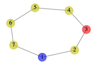
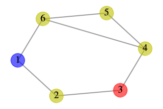
Figure 11: A $C_{7}$ graph (left) and a $C_{6}$ graph plus an extra edge between nodes $4$ and $6$ (right).

B.1 Non-oscillatory sources and sinks

In this section, we include more results from the simulations on cycle graphs of larger sizes and more general graph structure; see Figures 12 and 13. We observe that the slime mould model can still find the shortest path in both cases.

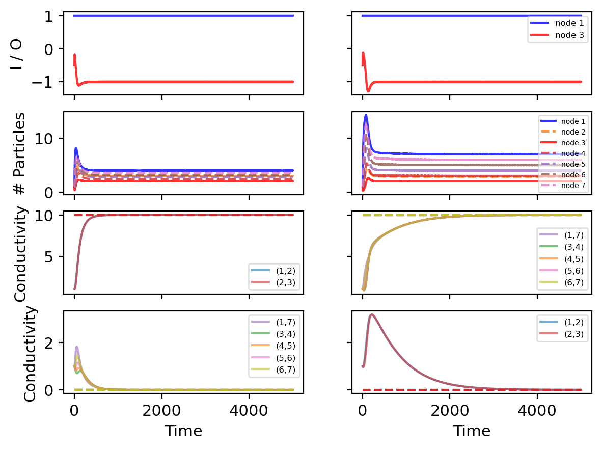
Figure 12: Results from the model on $C_{7}$ graph, with node $1$ as a source, node $3$ as a sink, an inflow at rate $a=1$, an outflow at rate $b=0.5$, and the lengths of all edges are $l_{ij}=10$ apart from $(1,2)$. On the left, we set $l_{12}=10$, thus path going through 1-2-3, is the shortest one. On the right, we set $l_{12}=50$, thus the path going through 1-7-6-5-4-3 is the shortest one. The first row shows the input at node $1$ and output at node $3$, the second row plots the number of particles on each node, $N_{i}(t)$, the third row indicates the conductivity of the edges in the shortest path, and the last row indicates the conductivity of the remaining edges in the graph, where the dashed lines in the corresponding color shows the analytical results of the steady state.

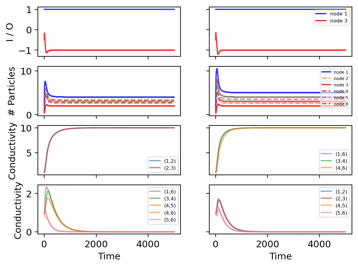
Figure 13: Results from the model on $C_{6}$ graph plus an extra edge between nodes 4 and 6 as the right in Figure 11, with node $1$ as a source, node $3$ as a sink, an inflow at rate $a=1$, an outflow at rate $b=0.5$, and the lengths of all edges are $l_{ij}=10$ apart from $(1,2)$. On the left, we set $l_{12}=10$, thus path going through 1-2-3, is the shortest one. On the right, we set $l_{12}=40$, thus the path going through 1-6-4-3 is the shortest one. The first row shows the input at node $1$ and output at node $3$, the second row plots the number of particles on each node, $N_{i}(t)$, the third row indicates the conductivity of the edges in the shortest path, and the last row indicates the conductivity of the remaining edges in the graph.

B.2 Oscillating nodes

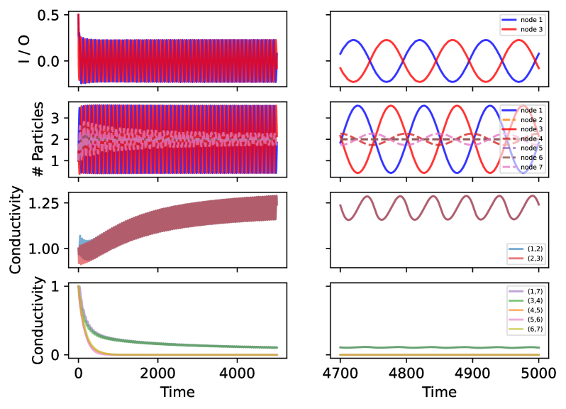
Figure 14: Results from the model on a $C_{7}$ graph, with nodes 1 and 3 as the oscillating nodes, rate $b=0.5$, amplitude $A_{1}=A_{3}=A=1$, frequency $\theta_{1}=\theta_{3}=\theta=0.01$, and phases $\phi_{1}=0$ and $\phi_{3}=\pi$, with the same reinforcement parameter $q=0.1$ and decay parameter $\lambda=0.01$ as in Figure 3. The first row plots the actual input/output to the two nodes, the second row shows the number of particles in each node, the third row indicates the conductivity of the edges in the shortest path and the last row indicates the conductivity of the remaining edges in the graph, with the full profile on the left while the change in the long term on the right.

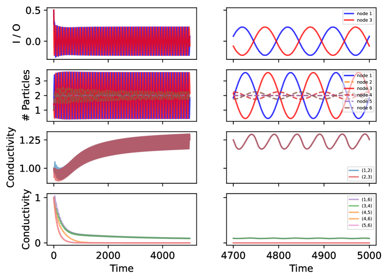
Figure 15: Results from the model on a $C_{6}$ graph plus an extra edge between nodes 4 and 6 as the right in Figure 11, with nodes 1 and 3 as the oscillating nodes, rate $b=0.5$, amplitude $A_{1}=A_{3}=A=1$, frequency $\theta_{1}=\theta_{3}=\theta=0.01$, and phases $\phi_{1}=0$ and $\phi_{3}=\pi$, with the same reinforcement parameter $q=0.1$ and decay parameter $\lambda=0.01$ as in Figure 3. The first row plots the actual input/output to the two nodes, the second row shows the number of particles in each node, the third row indicates the conductivity of the edges in the shortest path and the last row indicates the conductivity of the remaining edges in the graph, with the full profile on the left while the change in the long term on the right.

References

- [1] E. Başar, C. Başar-Eroğlu, S. Karakaş, and M. Schürmann, “Brain oscillations in perception and memory,” International journal of psychophysiology, vol. 35, no. 2-3, pp. 95–124, 2000.
- [2] K. Begus and E. Bonawitz, “The rhythm of learning: Theta oscillations as an index of active learning in infancy,” Developmental Cognitive Neuroscience, vol. 45, p. 100810, 2020.
- [3] N. A. Herweg, E. A. Solomon, and M. J. Kahana, “Theta oscillations in human memory,” Trends in cognitive sciences, vol. 24, no. 3, pp. 208–227, 2020.
- [4] A. Gnaedinger, H. Gurden, B. Gourévitch, and C. Martin, “Multisensory learning between odor and sound enhances beta oscillations,” Scientific Reports, vol. 9, no. 1, p. 11236, 2019.
- [5] S. Hanslmayr, J. Gross, W. Klimesch, and K. L. Shapiro, “The role of alpha oscillations in temporal attention,” Brain research reviews, vol. 67, no. 1-2, pp. 331–343, 2011.
- [6] J. E. Lisman and O. Jensen, “The theta-gamma neural code,” Neuron, vol. 77, no. 6, pp. 1002–1016, 2013.
- [7] O. Jensen, B. Gips, T. O. Bergmann, and M. Bonnefond, “Temporal coding organized by coupled alpha and gamma oscillations prioritize visual processing,” Trends in neurosciences, vol. 37, no. 7, pp. 357–369, 2014.
- [8] S. J. Martin, P. D. Grimwood, and R. G. Morris, “Synaptic plasticity and memory: an evaluation of the hypothesis,” Annual review of neuroscience, vol. 23, no. 1, pp. 649–711, 2000.
- [9] C. Hölscher, “Synaptic plasticity and learning and memory: Ltp and beyond,” Journal of neuroscience research, vol. 58, no. 1, pp. 62–75, 1999.
- [10] S. D. Fisher, P. B. Robertson, M. J. Black, P. Redgrave, M. A. Sagar, W. C. Abraham, and J. N. Reynolds, “Reinforcement determines the timing dependence of corticostriatal synaptic plasticity in vivo,” Nature communications, vol. 8, no. 1, p. 334, 2017.
- [11] T. Shindou, M. Shindou, S. Watanabe, and J. Wickens, “A silent eligibility trace enables dopamine-dependent synaptic plasticity for reinforcement learning in the mouse striatum,” European Journal of Neuroscience, vol. 49, no. 5, pp. 726–736, 2019.
- [12] M. Van Duijn, F. Keijzer, and D. Franken, “Principles of minimal cognition: Casting cognition as sensorimotor coordination,” Adaptive Behavior, vol. 14, no. 2, pp. 157–170, 2006.
- [13] P. Lyon, F. Keijzer, D. Arendt, and M. Levin, “Reframing cognition: getting down to biological basics,” 2021.
- [14] A. Boussard, A. Fessel, C. Oettmeier, L. Briard, H.-G. Döbereiner, and A. Dussutour, “Adaptive behaviour and learning in slime moulds: the role of oscillations,” Philosophical Transactions of the Royal Society B, vol. 376, no. 1820, p. 20190757, 2021.
- [15] M. Behar and A. Hoffmann, “Understanding the temporal codes of intra-cellular signals,” Current opinion in genetics & development, vol. 20, no. 6, pp. 684–693, 2010.
- [16] J. E. Purvis and G. Lahav, “Encoding and decoding cellular information through signaling dynamics,” Cell, vol. 152, no. 5, pp. 945–956, 2013.
- [17] F. Baluška and S. Mancuso, “Root apex transition zone as oscillatory zone,” Frontiers in Plant Science, vol. 4, p. 354, 2013.
- [18] J. Traas and T. Vernoux, “Oscillating roots,” Science, vol. 329, no. 5997, pp. 1290–1291, 2010.
- [19] C. Oettmeier, K. Brix, and H.-G. Döbereiner, “Physarum polycephalum—a new take on a classic model system,” Journal of Physics D: Applied Physics, vol. 50, no. 41, p. 413001, 2017.
- [20] J. Vallverdú, O. Castro, R. Mayne, M. Talanov, M. Levin, F. Baluška, Y. Gunji, A. Dussutour, H. Zenil, and A. Adamatzky, “Slime mould: the fundamental mechanisms of biological cognition,” Biosystems, vol. 165, pp. 57–70, 2018.
- [21] J. Smith-Ferguson and M. Beekman, “Who needs a brain? slime moulds, behavioural ecology and minimal cognition,” Adaptive Behavior, vol. 28, no. 6, pp. 465–478, 2020.
- [22] R. P. Boisseau, D. Vogel, and A. Dussutour, “Habituation in non-neural organisms: evidence from slime moulds,” Proceedings of the Royal Society B: Biological Sciences, vol. 283, no. 1829, p. 20160446, 2016.
- [23] T. Saigusa, A. Tero, T. Nakagaki, and Y. Kuramoto, “Amoebae anticipate periodic events,” Physical review letters, vol. 100, no. 1, p. 018101, 2008.
- [24] T. Nakagaki, H. Yamada, and Á. Tóth, “Maze-solving by an amoeboid organism,” Nature, vol. 407, no. 6803, pp. 470–470, 2000.
- [25] M. Beekman and T. Latty, “Brainless but multi-headed: decision making by the acellular slime mould physarum polycephalum,” Journal of molecular biology, vol. 427, no. 23, pp. 3734–3743, 2015.
- [26] A. Tero, S. Takagi, T. Saigusa, K. Ito, D. P. Bebber, M. D. Fricker, K. Yumiki, R. Kobayashi, and T. Nakagaki, “Rules for biologically inspired adaptive network design,” Science, vol. 327, no. 5964, pp. 439–442, 2010.
- [27] C. R. Reid, M. Beekman, T. Latty, and A. Dussutour, “Amoeboid organism uses extracellular secretions to make smart foraging decisions,” Behavioral Ecology, vol. 24, no. 4, pp. 812–818, 2013.
- [28] C. R. Reid and M. Beekman, “Solving the towers of hanoi–how an amoeboid organism efficiently constructs transport networks,” Journal of Experimental Biology, vol. 216, no. 9, pp. 1546–1551, 2013.
- [29] A. Takamatsu, T. Fujii, H. Yokota, K. Hosokawa, T. Higuchi, and I. Endo, “Controlling the geometry and the coupling strength of the oscillator system in plasmodium of physarum polycephalum by microfabricated structure,” Protoplasma, vol. 210, pp. 164–171, 2000.
- [30] A. Takamatsu, R. Tanaka, H. Yamada, T. Nakagaki, T. Fujii, and I. Endo, “Spatiotemporal symmetry in rings of coupled biological oscillators of physarum plasmodial slime mold,” Physical Review Letters, vol. 87, no. 7, p. 078102, 2001.
- [31] A. Dussutour, “Learning in single cell organisms,” Biochemical and Biophysical Research Communications, vol. 564, pp. 92–102, 2021.
- [32] R. D. Beer and J. C. Gallagher, “Evolving dynamical neural networks for adaptive behavior,” Adaptive behavior, vol. 1, no. 1, pp. 91–122, 1992.
- [33] R. D. Beer et al., “Toward the evolution of dynamical neural networks for minimally cognitive behavior,” From animals to animats, vol. 4, pp. 421–429, 1996.
- [34] N. Brancazio, “Easy alliances: The methodology of minimally cognitive behavior (mmcb) and basal cognition,” 2022.
- [35] J. Liu, R. Martinez-Corral, A. Prindle, D.-y. D. Lee, J. Larkin, M. Gabalda-Sagarra, J. Garcia-Ojalvo, and G. M. Süel Science, vol. 356, no. 6338, pp. 638–642, 2017.
- [36] L. L. Moroz, D. Y. Romanova, and A. B. Kohn, “Neural versus alternative integrative systems: molecular insights into origins of neurotransmitters,” Philosophical Transactions of the Royal Society B, vol. 376, no. 1821, p. 20190762, 2021.
- [37] G. Pezzulo, J. LaPalme, F. Durant, and M. Levin, “Bistability of somatic pattern memories: stochastic outcomes in bioelectric circuits underlying regeneration,” Philosophical Transactions of the Royal Society B, vol. 376, no. 1821, p. 20190765, 2021.
- [38] R. D. Beer, “Lost in words,” Adaptive Behavior, vol. 28, no. 1, pp. 19–21, 2020.
- [39] S. S. Schmieder, C. E. Stanley, A. Rzepiela, D. van Swaay, J. Sabotič, S. F. Nørrelykke, A. J. deMello, M. Aebi, and M. Künzler, “Bidirectional propagation of signals and nutrients in fungal networks via specialized hyphae,” Current Biology, vol. 29, no. 2, pp. 217–228, 2019.
- [40] H. V. Westerhoff, A. N. Brooks, E. Simeonidis, R. García-Contreras, F. He, F. C. Boogerd, V. J. Jackson, V. Goncharuk, and A. Kolodkin, “Macromolecular networks and intelligence in microorganisms,” Frontiers in microbiology, vol. 5, p. 379, 2014.
- [41] K. Y. Wan, “Active oscillations in microscale navigation,” Animal Cognition, pp. 1–14, 2023.
- [42] A. Tero, R. Kobayashi, and T. Nakagaki, “Physarum solver: A biologically inspired method of road-network navigation,” Physica A: Statistical Mechanics and its Applications, vol. 363, no. 1, pp. 115–119, 2006.
- [43] K. Ito, A. Johansson, T. Nakagaki, and A. Tero, “Convergence properties for the physarum solver,” arXiv preprint arXiv:1101.5249, 2011.
- [44] V. Bonifaci, K. Mehlhorn, and G. Varma, “Physarum can compute shortest paths,” Journal of theoretical biology, vol. 309, pp. 121–133, 2012.
- [45] S. Watanabe and A. Takamatsu, “Transportation network with fluctuating input/output designed by the bio-inspired physarum algorithm,” PloS one, vol. 9, no. 2, p. e89231, 2014.
- [46] Q. Ma, A. Johansson, A. Tero, T. Nakagaki, and D. J. Sumpter, “Current-reinforced random walks for constructing transport networks,” Journal of the Royal Society Interface, vol. 10, no. 80, p. 20120864, 2013.
- [47] Y. Kuramoto, “International symposium on mathematical problems in theoretical physics,” Lecture notes in Physics, vol. 30, p. 420, 1975.
- [48] M. Breakspear, S. Heitmann, and A. Daffertshofer, “Generative models of cortical oscillations: neurobiological implications of the kuramoto model,” Frontiers in human neuroscience, vol. 4, p. 190, 2010.
- [49] J. Cabral, E. Hugues, O. Sporns, and G. Deco, “Role of local network oscillations in resting-state functional connectivity,” Neuroimage, vol. 57, no. 1, pp. 130–139, 2011.
- [50] Y. L. Maistrenko, B. Lysyansky, C. Hauptmann, O. Burylko, and P. A. Tass, “Multistability in the kuramoto model with synaptic plasticity,” Physical Review E, vol. 75, no. 6, p. 066207, 2007.
- [51] L. Timms and L. Q. English, “Synchronization in phase-coupled kuramoto oscillator networks with axonal delay and synaptic plasticity,” Physical Review E, vol. 89, no. 3, p. 032906, 2014.
- [52] T. Ruangkriengsin and M. A. Porter, “Low-dimensional analysis of a kuramoto model with inertia and hebbian learning,” arXiv preprint arXiv:2203.12090, 2022.
- [53] K. Alim, N. Andrew, A. Pringle, and M. P. Brenner, “Mechanism of signal propagation in physarum polycephalum,” Proceedings of the National Academy of Sciences, vol. 114, no. 20, pp. 5136–5141, 2017.
- [54] A. Tero, R. Kobayashi, and T. Nakagaki, “A mathematical model for adaptive transport network in path finding by true slime mold,” Journal of theoretical biology, vol. 244, no. 4, pp. 553–564, 2007.
- [55] A. Tero, K. Yumiki, R. Kobayashi, T. Saigusa, and T. Nakagaki, “Flow-network adaptation in physarum amoebae,” Theory in biosciences, vol. 127, pp. 89–94, 2008.
- [56] S. Wiggins, Introduction to Applied Nonlinear Dynamical Systems and Chaos. New York: Springer, 1990.
- [57] M. Sims and J. Kiverstein, “Externalized memory in slime mould and the extended (non-neuronal) mind,” Cognitive Systems Research, vol. 73, pp. 26–35, 2022.
- [58] C. R. Reid, “Thoughts from the forest floor: a review of cognition in the slime mould physarum polycephalum,” Animal Cognition, pp. 1–15, 2023.
- [59] M. Ciszak, E. Masi, F. Baluška, and S. Mancuso, “Plant shoots exhibit synchronized oscillatory motions,” Communicative & integrative biology, vol. 9, no. 5, p. e1238117, 2016.
- [60] W. Ma, A. Trusina, H. El-Samad, W. A. Lim, and C. Tang, “Defining network topologies that can achieve biochemical adaptation,” Cell, vol. 138, no. 4, pp. 760–773, 2009.