Adaptive Scheduling for Adaptive Sampling in pos Taggers Construction

Abstract

We introduce an adaptive scheduling for adaptive sampling as a novel way of machine learning in the construction of part-of-speech taggers. The goal is to speed up the training on large data sets, without significant loss of performance with regard to an optimal configuration. In contrast to previous methods using a random, fixed or regularly rising spacing between the instances, ours analyzes the shape of the learning curve geometrically in conjunction with a functional model to increase or decrease it at any time. The algorithm proves to be formally correct regarding our working hypotheses. Namely, given a case, the following one is the nearest ensuring a net gain of learning ability from the former, it being possible to modulate the level of requirement for this condition. We also improve the robustness of sampling by paying greater attention to those regions of the training data base subject to a temporary inflation in performance, thus preventing the learning from stopping prematurely.

The proposal has been evaluated on the basis of its reliability to identify the convergence of models, corroborating our expectations. While a concrete halting condition is used for testing, users can choose any condition whatsoever to suit their own specific needs.

1 Introduction

The possibility of accessing massive amounts of data and the decline in the cost of disk storage have decisively contributed to the growing popularity of machine learning (ml) algorithms as the basis for modelling tasks in both the classification [31] and clustering [38] domains. However, managing large amounts of information is an expensive, time-consuming and non-trivial activity, especially when expert knowledge is needed. Furthermore, having access to vast data bases does not imply that ml algorithms must use them all and a subset is therefore preferred, provided it does not reduce the quality of the mined knowledge. Such observations then supply the same learning power with far less computational cost and allow the training process to be speeded up, whilst their nature and optimal size are rarely obvious. This justifies the interest of developing efficient sampling techniques, which involves anticipating the link between performance and experience regarding the accuracy of the system we are generating. At this point, correctness with respect to the working hypotheses and robustness against changes to them should be guaranteed in order to supply a practical solution. The former ensures the effectiveness of the proposed strategy in the framework considered, while the latter enables fluctuations in the learning conditions to be assimilated without compromising correctness, thus providing reliability to our calculations.

An area of work that is particularly sensitive to these inconveniences is natural language processing (nlp), the components of which are increasingly based on ml [3, 50]. This is due to the major effort required to create the labelled data sets used as a training basis to generate such tools, especially when they involve new application domains where resources are scarce or even non-existent. The problem is especially delicate in the case of part-of-speech (pos) tagging, the classification task that marks a word in a text (corpus) as corresponding to a particular pos, based on both its definition and its context. One reason for this is the complexity of both the annotation task and the relations to be captured from learning, but another is that it serves as a first step for other nlp functionalities such as parsing and semantic analysis, so errors at this stage can lower their performance [49]. All this makes up a popular experimentation field for introducing new ml facilities, particularly around sampling technology [4, 32, 43, 46, 56], as with the present work. In this context, we first examine in Section 2 the methodologies serving as inspiration to solve the question posed, as well as our contributions. Next, Section 3 reviews the mathematical basis necessary to support our proposal, which we present in Section 4. In Section 5, we describe the testing frame for the experiments illustrated in Section 6. Finally, Section 7 presents our final conclusions.

2 The state of the art

While the common goal is to choose a set of observations and determine whether it is large enough to reach the desirable learning performance, we characterize a sampling strategy according to three labels often compatible with each other. In light of the consideration or non-consideration of an expert opinion for selecting the sample, whether human or not, the algorithm is identified [14, 44] as active or non-active. Depending on the use or non-use of knowledge about the behaviour of the model to be generated, we distinguish [27] between dynamic and static sampling. We can finally differentiate [10] between adaptive, also called sequential [17] or progressive [57], and batch sampling when the size of the sample is determined iteratively in an online fashion or prior to commencing the selection task. In order to mark the end of the sequencing process, adaptive methods associate a halting condition. At all events, although these labels are not mutually exclusive, the scheduling strategy applied to a great extent conditions the sampling approach.

2.1 Sampling scheduling

Active sampling often associates an adaptive architecture, recruiting for annotation at each cycle only examples corresponding to near miss observations [59], i.e. negative ones that differ from the learned concept in a small number of significant points. This results in a two-stage procedure in which a reduced set of labelled cases is first collected to start a loop of selection and further reprocessing on the complete training data base until a stopping condition verifies. Most of this research focuses on pool-based active sampling, in which selection is made from a pool following two main schema: uncertainty [32] and query-by-committee [48]. The former uses a single classifier to select the observation on which it has the lowest certainty. Committee-based sampling converges to the optimal model more quickly [19] by considering a set of classifiers working on the principle of maximal disagreement among them. Unfortunately, active sampling is windowing [41] so its learning curves are notoriously ill-behaved on noisy data [40], increasing the amount of such random fluctuations on subsequent samples. Accordingly, performance often decreases as the process progresses [21] questioning, despite its apparent potential, its adoption [2]. For that reason we do not cover it in this work.

Focusing on non-active designs, static proposals determine the size of the sample from its representativeness of the training data base in terms of feature distributions. This can be done through simple procedures such as consideration of the complete set when the cost is affordable, a technique commonly known as trivial selection, or a part of this suggested by an omniscient oracle. The random selection of a fixed number or fraction of observations can also be considered. All of these are batch techniques for which, with the exception of the trivial approach, no formal interpretation for their correctness is possible. This justifies the recourse to adaptive methods, where the simplest and most common way to pick instances is again randomly [1]. Given an initial sample size and a schedule of sample size increments, new instances are then added until the distributions of both the sample and the training data base, are sufficiently similar. Alternatively, a fixed sequencing scheduling can be considered, typically by applying geometric [40] or arithmetic selection [27], also referred to as uniform selection [58]. In either case, static sampling uses statistical inference [8] to define the halting condition and, in fact, practitioners sometimes speak of statistically valid sampling to refer to it [27]. This makes it possible to derive a theoretically guaranteed sample size, sufficient to achieve a task with given confidence by using the so-called concentration bounds [11, 25], which provides a well-founded basis to introduce these kinds of techniques. So, its correctness and robustness have been formally demonstrated [17], its computational complexity analyzed [35], and its usefulness for scaling up learning algorithms in data mining applications proved [57]. Sadly, the number of instances can be overestimated or even unrealistic [33], making the static option less attractive.

All the above justifies the interest in the more flexible dynamic sampling. It is then possible to work guided by a model for the shape of the learning curve [28], which we assume slows to an almost horizontal slope at about the time when the true performance reaches its peak. This suggests a sequential scheduling such as those previously commented, which results in an adaptive philosophy, where at each cycle a model is built from the current sample and its performance evaluated. In this regard, arithmetic progressions can require an unreasonable number of iterations when a large number of cases is needed. In contrast, a geometric schedule quickly reach an appropriate sample size, while it may easily overfit local disruptions and thus stop ahead of time due to a momentary increase in performance [30], resulting in a fragil robustness.

Regarding the halting condition, we envisage two approaches in accordance with the consideration of predictive accuracy as an absolute stopping criterion [20] or as nothing more than a cost factor of an optimization problem stated in decision theory [26]. The first scenario involves identifying the final plateau of the learning curve in terms of functional convergence. Some procedures in this respect have become popular, such as local detection and learning curve estimation [27], or linear regression with local sampling [40], even if we have had to wait until recently [55] to dispose of a formally correct one. On the contrary, when sampling performance is understood as the search for a proper cost/benefit trade-off, the authors have recourse to statistically based strategies. Formally, they apply the principle of maximum expected utility (meu) [38]. This implies taking into account all effectiveness considerations, which depends on the degree of control exercised by the user on the learning process. In its absence, i.e. using non-active techniques as we do, the final cost is the sum of data acquisition, error and model induction charges [58]. Nonetheless, at best, heuristic techniques are used to calculate the first two and there is thus no way of guaranteeing the location of a global optimum [30], which often results in assuming fixed budgets [29]. That is why this kind of stopping criterion is not advisable to define reliable testing frames on sampling scheduling.

In practice, the success of adaptive sampling depends heavily on prior knowledge about the underlying model induction algorithm applied, which may be less than precise, thereby precipitating or delaying the detection of convergence and increasing the associated operating costs. Since this expertise can be obtained on the fly, the use of also adaptive scheduling seems to be better placed to achieve optimal results. It therefore becomes a question of rationally adjusting the number of cases between successive cycles. Surprisingly, to the best of our knowledge, the only action in this direction is due to Provost et al. [40]. From a set of instances large enough to obtain reliable estimates, they iteratively build models for both the convergence probability distribution and the run-time complexity of the underlying induction algorithm. At each cycle the convergence is checked and, if it does not occur, the schedule is rebuilt from the latest information and the process restarts. However, this proposal performs in practice much worse than the less complicated geometric one, which seems to have discouraged further research on this topic, despite its vast potential.

2.2 Our contribution

We introduce an adaptive scheduling, baptized as colts, with a view to reducing operating charges in non-active adaptive sampling. The idea is to calculate, at each iteration, the smallest amount of training data to be added for ensuring that the next case is relevant in learning terms. From a set of usual working hypotheses in ml, the technique is described taking an exclusively geometrical point of view. Once a sequence of observations has been set, a functional approximation to the associated partial learning curve is built. The next instance from which a new observation to update our evaluation is mandatory, i.e. from which the working hypotheses can no longer be guaranteed, is then located. We do this by calculating the case the degree of concavity, namely the learning speed, which cannot be maintained over time on the real learning curve. The correctness of the method is formally established and its robustness explored.

The proposal is evaluated within a uniform testing framework, in the sense that its standards of evidence do not favour any particular sampling scheduling, taking the generation of pos taggers as a case study. Once a learner, a halting condition and a training data base are fixed, the aim is to categorize a set of schedules according to their efficiency to achieve a given level of accuracy in the model being generated. To that end, predictive accuracy is taken as the stopping criterion, thereby avoiding the inconveniences associated with meu-based halting conditions. We also introduce the metric used as an assessment basis, together with its associated monitoring architecture for data collection. The latter captures the concept of testing round (run), which serves to normalize the conditions under which the experiments take place. Thus, runs only distinguishable by their scheduling strategy are grouped around an item acting as baseline, in what we call a local testing frame. It then becomes possible to compare, within these structures, runs in terms of both training resources used and overall learning costs. By doing so, we avoid recourse to cumbersome heuristics, often highly dependent on the knowledge domain considered, endowing the tests with reliability and safety.

3 The formal framework

The aim is to introduce the mathematical basis that enables to prove the correctness of our proposal. Most of these formal notions are taken from Vilares et al. [55], denoting the set of real numbers by $\mathbb{R}$ and that of naturals by $\mathbb{N}$, assuming that $0\not\in\mathbb{N}$. Another preliminary question to be clarified, because the generation of ml-based pos taggers serves as illustration guide, is the identification of the accuracy concept usually accepted in that kind of model. We define it as the number of correctly tagged tokens divided by the total ones, expressed as a percentage [54] and calculated following some generally admitted usages: all tokens are counted, including punctuation marks, and it is supposed that only one tag per token is provided.

3.1 The working hypotheses

We start with a sequence of observations calculated from cases incrementally taken from a training data base, meeting some conditions to ensure a predictable progression of the estimates over a virtually infinite interval. So, they are assumed to be independently and identically distributed [17, 47, 50]. We then accept that a learning curve is a positive definite and strictly increasing function on $\mathbb{N}$, where numbers are the positions of instances in the training data set, and upper bounded by 100. This results in a concave graph with horizontal asymptote.

Such hypotheses make up an idealized working frame to support correctness, while real learners may deviate from it, justifying a later study of robustness. These deviations translate into irregularities in both concavity and increase of the learning curves, as shown in the left-most diagram of Fig. 1 for the training of the fast transformation-based learning (fntbl) tagger [39] on the Freiburg-Brown (frown) corpus of American English [36]. The cases are therefore indexed by the position of a word in the text.

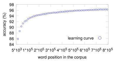
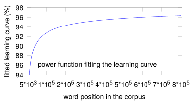
Figure 1: Learning curve for fntbl on frown, and an accuracy pattern fitting it.

3.2 The notational support

Having identified the working hypotheses, we need to formalize the data structures we are going to work with, such as the progressive sequence of instances whose selection we want to optimize.

Definition 1.

Let ${\mathcal{D}}$ be a training data base, $\mathcal{K}\subsetneq\mathcal{D}$ a subset of initial items from $D$ and $\sigma\!\in\!\Sigma\!:=\{\zeta:\mathbb{N}\rightarrow\mathbb{N}\}$ a function. We define a learning scheme for $\mathcal{D}$ with kernel ${\mathcal{K}}$ and step $\sigma$, as a triple $\mathcal{D}^{\mathcal{K}}_{\sigma}=[\mathcal{K},\sigma,\{\mathcal{D}_{i}\}_{i\in\mathbb{N}}]$ with $\{\mathcal{D}_{i}\}_{i\in\mathbb{N}}$ a cover of $\mathcal{D}$ verifying:

$${\mathcal{D}}_{1}:={\mathcal{K}}\mbox{ and }{\mathcal{D}}_{i}:={\mathcal{D}}_{i-1}\cup{\mathcal{I}}_{i},\;\mathcal{I}_{i}\subset{\mathcal{D}}\setminus{\mathcal{D}}_{i-1},\;\left\|{\mathcal{I}}_{i}\right\|=\sigma(i),\;\forall i\geq 2$$ (1)

where $\left\|{\mathcal{I}}_{i}\right\|$ is the cardinality of ${\mathcal{I}}_{i}$. We refer to $\mathcal{D}_{i}$ as the individual of level $i$ for $\mathcal{D}^{\mathcal{K}}_{\sigma}$.

A learning scheme relates a level $i$ with the position $\left\|\mathcal{D}_{i}\right\|$ in the training data base, determining the sequence of observations $\{[x_{i},{\mathcal{A}}_{\boldsymbol{\boldsymbol{\infty}}{}}[{\mathcal{D}}](x_{i})],\;x_{i}:=\left\|\mathcal{D}_{i}\right\|\}_{i\in\mathbb{N}}$, where ${\mathcal{A}}_{\boldsymbol{\boldsymbol{\infty}}{}}[{\mathcal{D}}](x_{i})$ is the accuracy achieved on such instance by the learner. Thus, a level determines an iteration in the adaptive sampling whose learning curve is ${\mathcal{A}}_{\boldsymbol{\boldsymbol{\infty}}{}}[{\mathcal{D}}]$, whilst ${\mathcal{K}}$ delimits a portion of ${\mathcal{D}}$ we believe to be enough to initiate consistent evaluations of the training. For its part, $\sigma$ identifies the sampling scheduling. As we want to address the latter from geometrical criteria, we need to extrapolate the partial learning curves according to a functional pattern providing stability to the estimates. The focus is on curves that verify the working hypotheses, but are also infinitely differentiable over the training domain. This supplies graphs without disruptions due to instantaneous jumps while ensuring their regularity.

Definition 2.

Let $C^{\infty}_{(0,\infty)}$ be the C-infinity functions in $\mathbb{R}^{+}$, we say that $\pi:\mathbb{R}^{{+}^{n}}\rightarrow C^{\infty}_{(0,\infty)}$ is an accuracy pattern iff $\pi(a_{1},\dots,a_{n})$ is positive definite, upper bounded, concave and strictly increasing.

An example of accuracy pattern is the power family of curves $\pi(a,b,c)(x):=-a*x^{-b}+c$, hereafter used as running one. Its upper bound is the horizontal asymptote value $\lim\limits_{x\rightarrow\infty}\pi(a,b,c)(x)=c$, and

$$\pi(a,b,c)^{\prime}(x)=a*b*x^{-(b+1)}>0\hskip 21.33955pt\pi(a,b,c)^{\prime\prime}(x)=-a*b*(b+1)*x^{-(b+2)}<0$$ (2)

which guarantees increase and concavity in $\mathbb{R}^{+}$, respectively. This is illustrated in the right-most diagram of Fig. 1, whose goal is to fit the learning curve represented in the left-hand side. Here, the values $a=542.5451$, $b=0.3838$ and $c=99.2876$ are provided by the trust region method [5], a regression technique minimizing the summed square of residuals, i.e. the differences between the observed values and the fitted ones. Furthermore, as it is intended to determine from the current case the next one ensuring significance for learning, such a concept of usefulness must be formalized. To do it, we need to evaluate the progression of accuracy during the training process, which results in studying the sequence of curves modelled from the partial learning ones.

Definition 3.

Let $\mathcal{D}^{\mathcal{K}}_{\sigma}$ be a learning scheme, $\pi$ an accuracy pattern and $\ell\in\mathbb{N},\;\ell\geq 3$ a position in the training data base $\mathcal{D}$. We define the learning trend of level $\ell$ for ${\mathcal{D}}^{\mathcal{K}}_{\sigma}$ using $\pi$, as a curve ${\mathcal{A}}_{\ell}^{\pi}[{\mathcal{D}}^{\mathcal{K}}_{\sigma}]\in\pi$, fitting the observations $\{[x_{i},{\mathcal{A}}_{\boldsymbol{\boldsymbol{\infty}}{}}[{\mathcal{D}}](x_{i})],\;x_{i}:=\left\|\mathcal{D}_{i}\right\|\}_{i=1}^{\ell}$. A sequence of learning trends ${\mathcal{A}}^{\pi}[{\mathcal{D}}^{\mathcal{K}}_{\sigma}]:=\{{\mathcal{A}}_{\ell}^{\pi}[{\mathcal{D}}^{\mathcal{K}}_{\sigma}]\}_{\ell\in\mathbb{N}}$ is called a learning trace. We refer to $\{\alpha_{\ell}\}_{\ell\in\mathbb{N}}$ as the asymptotic backbone of ${\mathcal{A}}^{\pi}[{\mathcal{D}}^{\mathcal{K}}_{\sigma}]$, where $y=\alpha_{\ell}:=\lim\limits_{x\rightarrow\infty}{\mathcal{A}}_{\ell}^{\pi}[{\mathcal{D}}^{\mathcal{K}}_{\sigma}](x)$ is the asymptote of ${\mathcal{A}}_{\ell}^{\pi}[{\mathcal{D}}^{\mathcal{K}}_{\sigma}]$.

A learning trend ${\mathcal{A}}_{\ell}^{\pi}[{\mathcal{D}}^{\mathcal{K}}_{\sigma}]$ requires a level $\ell\geq 3$, because we need at least three observations to generate a curve. Its value ${\mathcal{A}}_{\ell}^{\pi}[{\mathcal{D}}^{\mathcal{K}}_{\sigma}](x_{i})$ represents the prediction for accuracy on a case $x_{i}$, using a model generated from the first $\ell$ iterations of the learner. Accordingly, the asymptotic term $\alpha_{\ell}$ is nothing other than the estimate for the highest accuracy attainable. This way, a learning trace gives a comprehensive picture of the increase in accuracy due to new observations, as well as future expectations in that respect. Continuing with the tagger fntbl and the corpus frown, Fig. 2 shows (left) a portion of the learning trace with kernel and uniform step function $5*10^{3}$, also including the real learning curve and a zoom view (right). As our running frame is the generation of pos taggers, levels are hereafter indicated by word positions in the training corpus. At this point, we are ready to capture the notion of learning utility associated to a case.

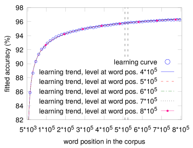
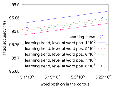
Figure 2: Learning trace for fntbl on frown.

Definition 4.

Let ${\mathcal{A}}^{\pi}[{\mathcal{D}}^{\mathcal{K}}_{\sigma}]$ be a learning trace and $\ell\in\mathbb{N},\;\ell\geq 3$. We say that $x_{\ell+1}$ is relevant for ${\mathcal{A}}^{\pi}[{\mathcal{D}}^{\mathcal{K}}_{\sigma}]$ iff ${\mathcal{A}}_{\ell}^{\pi}[{\mathcal{D}}^{\mathcal{K}}_{\sigma}]^{\prime}(x_{\ell})\neq{\mathcal{A}}_{\ell+1}^{\pi}[{\mathcal{D}}^{\mathcal{K}}_{\sigma}]^{\prime}(x_{\ell+1})$, with $x_{\ell}:=\left\|\mathcal{D}_{\ell}\right\|$.

A case is relevant when the slope of its learning trend at that point varies with regard to what happens in the previous instance. This reveals a change in the learning speed, i.e. in the degree of concavity, observed on the learning curve we try to approximate. We are therefore talking about an effective step towards the identification of convergence for training, providing a practical sense to the notion of relevance.

4 The abstract model

We lay the theoretical foundations of our proposal to later interpret them from an operational point of view. The first objective is to establish its correctness, i.e. to formalize a sampling scheduling for which the distance between two consecutive cases is the shortest one guaranteeing the relevance of the most recent instance. All that is required for such a purpose is to state the adequate step function.

4.1 Correctness

Given ${\mathcal{D}}$ a training data base, the goal is to identify the step function $\sigma$ under the terms outlined above, taking into account that excessively short steps can unnecessarily overload the sampling procedure, as with those regions in $\mathcal{D}$ on which the slope of the learning curve does not vary much.

Theorem 1.

Let ${\mathcal{A}}^{\pi}[{\mathcal{D}}^{\mathcal{K}}_{\sigma}]$ be a learning trace, then:

$$\forall i\geq 3,\;\sigma(i+1)\geq\frac{\alpha_{i}-{\mathcal{A}}_{i}^{\pi}[{\mathcal{D}}^{\mathcal{K}}_{\sigma}](x_{i})}{{\mathcal{A}}_{i}^{\pi}[{\mathcal{D}}^{\mathcal{K}}_{\sigma}]^{\prime}(x_{i})}\Rightarrow{\mathcal{A}}_{i+1}^{\pi}[{\mathcal{D}}^{\mathcal{K}}_{\sigma}]^{\prime}(x_{i+1})\neq{\mathcal{A}}_{i}^{\pi}[{\mathcal{D}}^{\mathcal{K}}_{\sigma}]^{\prime}(x_{i})$$ (3)

with $x_{i}:=\left\|\mathcal{D}_{i}\right\|$, and $y=\alpha_{i}$ the horizontal asymptote for ${\mathcal{A}}_{i}^{\pi}[{\mathcal{D}}^{\mathcal{K}}_{\sigma}]$.

Proof 1.

Suppose a learning trend ${\mathcal{A}}_{i}^{\pi}[{\mathcal{D}}^{\mathcal{K}}_{\sigma}]$ with $i\geq 3$, as shown in Fig. 3. Given that it is monotonic increasing (resp. concave), no point on it has an ordinate (resp. slope) greater than $\alpha_{i}$ (resp. ${\mathcal{A}}_{i}^{\pi}[{\mathcal{D}}^{\mathcal{K}}_{\sigma}]^{\prime}(x_{i})$) in the interval $(0,\infty)$ (resp. $(x_{i},\infty)$). Accordingly, the slope of ${\mathcal{A}}_{i}^{\pi}[{\mathcal{D}}^{\mathcal{K}}_{\sigma}]$ on $x_{i}$ cannot be maintained beyond the point indicated by the abscissa of $s_{i}$, the intersection point between its tangent line thorough $r_{i}$ and its horizontal asymptote. Since this abscissa is calculated substituting $y=\alpha_{i}$ in the tangent

$$y={\mathcal{A}}_{i}^{\pi}[{\mathcal{D}}^{\mathcal{K}}_{\sigma}]^{\prime}(x_{i})\ast(x-x_{i})+{\mathcal{A}}_{i}^{\pi}[{\mathcal{D}}^{\mathcal{K}}_{\sigma}](x_{i})$$ (4)

we have that $s_{i}=(\frac{\alpha_{i}-{\mathcal{A}}_{i}^{\pi}[{\mathcal{D}}^{\mathcal{K}}_{\sigma}](x_{i})}{{\mathcal{A}}_{i}^{\pi}[{\mathcal{D}}^{\mathcal{K}}_{\sigma}]^{\prime}(x_{i})}+x_{i},\alpha_{i})$, from which we conclude the thesis. $\blacksquare$

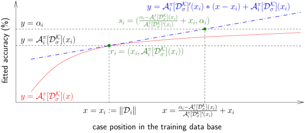
Figure 3: Computing dynamically the size of individuals in a learning trace.

We now have a sufficient condition to identify at each sampling cycle the closest instance from which a real impact on learning capacity is ensured, because the step applied guarantees its relevance. However, this does not exclude the possibility that smaller steps could eventually produce the same effect. Thus, the probability of a case being relevant is proportional to the value proposed, an idea that is useful to formalize.

Definition 5.

Let ${\mathcal{A}}^{\pi}[{\mathcal{D}}^{\mathcal{K}}_{\sigma}]$ be a learning trace, its probability of relevant training (port) at level $i\geq 4$ is

$$\varrho(i):=\left\{\begin{array}[]{ll}1&\mbox{\em if}\;\sigma(i)\geq\mu(i)\\ \sigma(i)/\mu(i)&\mbox{\em otherwise}\end{array}\right.,\;\mu(i):=\frac{\alpha_{i}-{\mathcal{A}}_{i}^{\pi}[{\mathcal{D}}^{\mathcal{K}}_{\sigma}](x_{i})}{{\mathcal{A}}_{i}^{\pi}[{\mathcal{D}}^{\mathcal{K}}_{\sigma}]^{\prime}(x_{i})},\;x_{i}:=\left\|{\mathcal{D}}_{i}\right\|$$ (5)

Following Theorem 1, $\mu(i)$ is the shortest separation that guarantees the relevance of the case at level $i$. Consequently, any step $\sigma(i)\geq\mu(i)$ corresponds to a maximal port, whereas the low distances are associated with proportional values. Since step functions are strictly positive definite, the port is defined in the interval $(0,1]$ and provides a simple mechanism to regulate, in probabilistic terms, the interrelation between the speed of learning and the training sequence in a learning trace. This allows us to immediately prove the correctness of a sample with respect to a given port.

Theorem 2.

(Correctness) Let ${\mathcal{A}}^{\pi}[{\mathcal{D}}^{\mathcal{K}}_{\sigma[\varrho]}]$ be a learning trace and $\sigma[\varrho]$ the step function

$$\sigma[\varrho](i):=\left\lceil\varrho\ast\frac{\alpha_{i}-{\mathcal{A}}_{i}^{\pi}[{\mathcal{D}}^{\mathcal{K}}_{\sigma[\varrho]}](x_{i})}{{\mathcal{A}}_{i}^{\pi}[{\mathcal{D}}^{\mathcal{K}}_{\sigma[\varrho]}]^{\prime}(x_{i})}\right\rceil,\;\varrho\in(0,1],\;x_{i}:=\left\|{\mathcal{D}}_{i}\right\|,\;\forall i\geq 4$$ (6)

with $y=\alpha_{i}$ the horizontal asymptote for ${\mathcal{A}}_{i}^{\pi}[{\mathcal{D}}^{\mathcal{K}}_{\sigma[\varrho]}]$ and $\left\lceil x\right\rceil$ the ceiling function mapping $x\in\mathbb{R}$ to the supremum in $[x,\infty)\cap\mathbb{N}$. Then, ${\mathcal{A}}^{\pi}[{\mathcal{D}}^{\mathcal{K}}_{\sigma[\varrho]}]$ has the smallest port greater than or equal to $\varrho$.

Proof 2.

Trivial from Theorem 1. $\blacksquare$

We can hence categorize the step functions according to their ability to minimize, with regard to a port value, the amount of training data to be added in each iteration of a progressive sampling process. Thus, once a port value $\varrho$ has been determined, the step function we are looking for is given by $\sigma[\varrho]$. We turn again to the running example to illustrate the potential of this outcome in Fig. 4, including both a general and a zoom view. The learning curve is the same as that considered in Fig. 2, the observations of which we now compare with two learning trends whose levels correspond approximately to the same position in the corpus ($\sim 4.95*10^{5}$), using identical kernel size ($5*10^{3}$) and computed from different step functions: a uniform spacing $\sigma=5*10^{3}$ and an adaptive one $\sigma[0.01]$. The latter provides a better use of the training process by reducing the number of cases without appreciably affecting the quality of the estimates for accuracy. In any event, it is important to note that the correctness has been stated from the working hypotheses, which relate to an ideal conceptualization of the learning curves that may be subject to variations in practice. We therefore need to analyze mechanisms for achieving robustness of sampling.

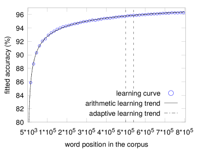
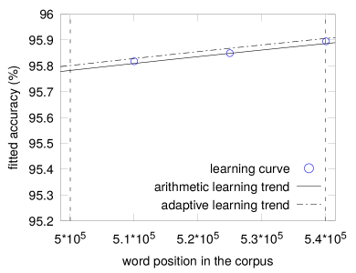
Figure 4: Learning trends for fntbl on frown, using uniform and adaptive step functions.

4.2 Robustness

This study requires the review of our working hypotheses in order to accommodate the notion of irregular observation in real-world ml. We then assume that learning curves are positive definite and upper bounded by 100, conditions guaranteed, but only quasi-strictly increasing and concave. These are our testing hypotheses and, given that the questions to be addressed are common, we entrust the treatment of robustness to the mechanisms intended to enhance it in the definition of the halting condition. On this point, although any of the solutions in the state of the art could be applied, we raise the subject in the context of the layered convergence criterion [55], which we briefly recall now. The choice is justified for reasons of both theoretical and practical order, conjugating a formally correct proposal with a high level of performance and a simple start-up. Furthermore, the approach is easy to interpret in terms of learning traces, thus facilitating rapid understanding. In fact, because they are not part of our contributions but mere discussion tools, the reader can leave out the formal definitions and results in the remainder of this Section to focus on the intuitive interpretation accompanying them.

We identify two types of irregular observations according to their position in relation to the working level (wlevel), i.e. the iteration from which they would have a small enough impact to work in their softening. As this depends on unpredictable factors such as the magnitude, distribution and the very existence of these disorders, a formal characterization is impossible and a heuristic is necessary. Assuming that the model stabilizes as the training advances, a way of addressing the question is categorizing the variations induced in the monotony of the asymptotic backbone, at the basis of the correctness for any halting condition, to locate the level providing the first one below a given ceiling. Once the wlevel passed, we are interested in estimates beyond the prediction level (plevel) marking the likely beginning to learn trends which could feasibly predict the learning curve, therefore not exceeding its maximum (100).

Definition 6.

Let ${\mathcal{A}}^{\pi}[{\mathcal{D}}^{\mathcal{K}}_{\sigma}]$ be a learning trace with asymptotic backbone $\{\alpha_{i}\}_{i\in\mathbb{N}}$, $\nu\in(0,1)$, $\varsigma\in\mathbb{N}$ and $\lambda\in\mathbb{N}\cup\{0\}$. We define the working level (wlevel) for ${\mathcal{A}}^{\pi}[{\mathcal{D}}^{\mathcal{K}}_{\sigma}]$ with verticality threshold $\nu$, slowdown $\varsigma$ and look-ahead $\lambda$, as the smallest $\omega(\nu,\varsigma,\lambda)\in\mathbb{N}$ verifying

$$\frac{\sqrt[\varsigma]{\nu}}{1-\nu}\geq\frac{\mid\alpha_{i+1}-\alpha_{i}\mid}{x_{i+1}-x_{i}},\;x_{i}:=\left\|{\mathcal{D}}_{i}\right\|,\;\forall i\in\mathbb{N}\;\mbox{ such that }\;\omega(\nu,\varsigma,\lambda)\leq i\leq\omega(\nu,\varsigma,\lambda)+\lambda$$ (7)

while the smallest $\wp(\nu,\varsigma,\lambda)\geq\omega(\nu,\varsigma,\lambda)$ with $\alpha_{\wp(\nu,\varsigma,\lambda)}\leq 100$ is the prediction level (plevel). Unless they are necessary for understanding, we shall omit the parameters, referring to wlevel by $\omega$ (resp. plevel by $\wp$).

The wlevel is the first level for which the normalized absolute value of the slope of the line joining consecutive points on the asymptotic backbone is less than the verticality threshold $\nu$, which is corrected by a factor $1/\varsigma$ in order to slow down the normalization pace, thus helping to avoid the use of infinitely small numerals for $\nu$ in real applications. Since those tangential values decrease together with the deviations in the monotony studied, we use this correlation to categorize the latter, taking the look-ahead $\lambda$ as our verification window. We then place plevel on the first cycle with a learning trend below 100. In our example, the differences of scale between disruptions in the monotony of the asymptotic backbone before and after the wlevel are shown in the left-most diagram of Fig. 5 for the parameters $\nu=2*10^{-5}$, $\varsigma=1$ and $\lambda=5$.

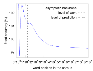
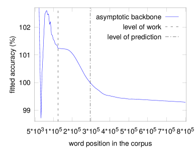
Figure 5: Working and prediction levels for fntbl on frown.

4.2.1 Irregularities before the working level

The few observations available, combined with the steep slopes of the asymptotic backbone, have here a multiplying effect on the fluctuations of its monotony. The use of large enough samples would mitigate the problem, but identifying the optimal sampling size for such purpose is equivalent to estimate the wlevel. So, the only effective strategy to avoid such alterations is to discard trends associated to pre-working levels, as reflected in the left-most diagram of Fig. 5.

4.2.2 Irregularities after the working level

These should be below the verticality threshold, facilitating the restoration of the asymptotic backbone by using an extra observation, called anchor, at the point of infinity of each learning trend. Since the sum total of residuals in any of those curves is null, this may help to neutralize irregularities. Thus, anchoring integrates naturally into the concept of learning trace as a mechanism to improve its robustness.

Definition 7.

Let ${\mathcal{A}}^{\pi}[{\mathcal{D}}^{\mathcal{K}}_{\sigma}]$ be a learning trace with wlevel $\omega$, and the sequence $\{\hat{\mathcal{A}}_{\ell}(\infty)\}_{\ell>\omega}$ in $\mathbb{R}^{+}$. A learning trend of level $\ell>\omega$ with anchor $\hat{\mathcal{A}}_{\ell}(\infty)$ for ${\mathcal{A}}_{\boldsymbol{\boldsymbol{\infty}}{}}[{\mathcal{D}}]$ using the accuracy pattern $\pi$, is a curve $\hat{\mathcal{A}}_{\ell}^{\pi}[{\mathcal{D}}^{\mathcal{K}}_{\sigma}]\in\pi$ fitting the observations $\{[x_{i},{\mathcal{A}}_{\boldsymbol{\boldsymbol{\infty}}{}}[{\mathcal{D}}](x_{i})],\;x_{i}:=\left\|\mathcal{D}_{i}\right\|\}_{i=1}^{\ell}\cup\;[\infty,\hat{\mathcal{A}}_{\ell}(\infty)]$, whose asymptote is denoted by $y=\hat{\alpha}_{\ell}$. When $\{\hat{\alpha}_{\ell}\}_{\ell>\omega}$ is positive definite and converges monotonically to the asymptotic value $\alpha_{\boldsymbol{\boldsymbol{\infty}}{}}$ of ${\mathcal{A}}_{\boldsymbol{\boldsymbol{\infty}}{}}[{\mathcal{D}}]$, we say that $\hat{\mathcal{A}}^{\pi}[{\mathcal{D}}^{\mathcal{K}}_{\sigma}]:=\{\hat{\mathcal{A}}_{\ell}^{\pi}[{\mathcal{D}}^{\mathcal{K}}_{\sigma}]\}_{\ell>\omega}$ is an anchoring learning trace of reference $[{\mathcal{A}}^{\pi}[{\mathcal{D}}^{\mathcal{K}}_{\sigma}],\omega]$.

Effectively, an anchor is treated as another observation and located as far as the computer memory allows, which is why its use does not modify the properties of standard learning traces. In particular, the correctness of the proximity condition determining the level from which the learning trends estimate the accuracy below an error threshold [55], is extended in a natural way. It thus provides a simple criterion to stop a training process, while the anchors give robustness. For ensuring its full practical implementation, the condition is relaxed to define it in terms of the net contribution of each learning trend to the convergence. We then characterize the level from which such an accuracy gain, baptized as layer of convergence, is lower than a ceiling fixed by the user.

Theorem 3.

(Layered Correctness) Let ${\mathcal{A}}^{\pi}[{\mathcal{D}}^{\mathcal{K}}_{\sigma}]$ be a (resp. anchoring) learning trace with asymptotic backbone $\{\alpha_{i}\}_{i\in\mathbb{N}}$. We then have that

$$\forall\varepsilon>0,\;\exists n\in\mathbb{N},\mbox{ such that }[\chi({\mathcal{A}}_{i}^{\pi}[{\mathcal{D}}^{\mathcal{K}}_{\sigma}])\leq\varepsilon\Leftrightarrow i\geq n]$$ (8)

where $\chi({\mathcal{A}}_{i}^{\pi}[{\mathcal{D}}^{\mathcal{K}}_{\sigma}]):=\mid{\mathcal{A}}_{i}^{\pi}[{\mathcal{D}}^{\mathcal{K}}_{\sigma}](x_{i})-\alpha_{i}\mid$ is the layer of convergence for ${\mathcal{A}}_{i}^{\pi}[{\mathcal{D}}^{\mathcal{K}}_{\sigma}],\;x_{i}:=\left\|{\mathcal{D}}_{i}\right\|,\;\forall\;i\in\mathbb{N}$.

Proof 3.

See in [55]. $\blacksquare$

At this point, our sole outstanding issue is how to generate anchors and show their effect in practice. Our thinking is based on the fact that, having fixed a learning trend, the degree of reduction applicable to the irregularities correlates with its residual at the point of infinity. Extending this logic further, the closer to the asymptote of the learning trend, the better its anchor. The problem is that to optimize the latter we need to compute the former and vice versa, leading us into a vicious circle. A way to avoid this is to assign the anchor at a given level to the asymptotic value of the previous learning trend, i.e. the last estimate available for the accuracy resulting from a virtually infinite training process. In return for the surrender of part of the correction potential, which gives the strategy a conservative character, the situation is thus unblocked to inspire the notion of canonical anchoring.

Theorem 4.

Let ${\mathcal{A}}^{\pi}[{\mathcal{D}}^{\mathcal{K}}_{\sigma}]$ be a learning trace with asymptotic backbone $\{\alpha_{i}\}_{i\in\mathbb{N}}$ and $\{\hat{\mathcal{A}}_{i}(\infty)\}_{i>\omega}$ the sequence defined from its wlevel $\omega$ as

$$\hat{\mathcal{A}}_{\omega+1}(\infty):=\alpha_{\omega}\hskip 21.33955pt\hat{\mathcal{A}}_{i+1}(\infty):=\hat{\alpha}_{i}:=\lim\limits_{x\rightarrow\infty}\hat{\mathcal{A}}_{i}^{\pi}[{\mathcal{D}}^{\mathcal{K}}_{\sigma}](x)$$ (9)

with $\hat{\mathcal{A}}_{i}^{\pi}[{\mathcal{D}}^{\mathcal{K}}_{\sigma}]$ a curve fitting $\{[x_{j},{\mathcal{A}}_{\boldsymbol{\boldsymbol{\infty}}{}}[{\mathcal{D}}](x_{j})],\;x_{j}:=\left\|\mathcal{D}_{j}\right\|\}_{j=1}^{i}\cup\;[\infty,\hat{\mathcal{A}}_{i}(\infty)]$, $\forall i>\omega$. Then $\alpha_{\omega+i}\leq\hat{\alpha}_{\omega+i}$ (resp. $\alpha_{\omega+i}\geq\hat{\alpha}_{\omega+i}$), $\forall i\in\mathbb{N}$, when $\{\alpha_{i}\}_{i\in\mathbb{N}}$ is decreasing (resp. increasing). Also, $\{\hat{\mathcal{A}}_{i}^{\pi}[{\mathcal{D}}^{\mathcal{K}}_{\sigma}]\}_{i>\omega}$ is an anchoring learning trace of reference $[{\mathcal{A}}^{\pi}[{\mathcal{D}}^{\mathcal{K}}_{\sigma}],\omega]$, with $\{\hat{\mathcal{A}}_{i}(\infty)\}_{i>\omega}$ its canonical anchors.

Proof 4.

See in [55]. $\blacksquare$

The effect of canonical anchoring in smoothing irregularities after the wlevel is illustrated, on our running example, in the right-most diagram of Fig. 5 versus its absence in the left-most one. It also shows how this technique, due to its conservative nature, slows down the learning convergence.

5 The testing frame

The focus is now on providing evidence of the interest in using our proposal in a non-active adaptive sampling context, from both points of view: training resources and learning costs. To support this, we design a categorizing protocol for scheduling strategies from the performance observed to converge below a given error threshold. The access to a proximity condition for marking the end of a learning process is then mandatory, a task we entrust to the layered convergence criterion whose correctness was established in Theorem 3. We also need quality metrics, which in turn require a specific monitoring architecture.

5.1 The monitoring architecture

After setting a ml task for a learner on a training data base ${\mathcal{D}}$, the goal is to standardize the conditions under which testing takes place, with a view to allow for its objective assessment. Since we are talking about sampling efficiency, the true location of the instance on which the intended effect fulfills, hereinafter called convergence case (ccase), should play a key role in our proposal. This identifies our first objective.

Let us assume an accuracy pattern $\pi$, a kernel $\mathcal{K}$ and a convergence threshold $\tau$. A way to approximate ccase is by calculating the instance related to the convergence level (clevel) of ${\mathcal{A}}^{\pi}[{\mathcal{D}}^{\mathcal{K}}_{\eta}]$, a learning trace associated to the selected ml task, with $\eta\in\mathbb{N}$ held to be fine enough. Namely, the iteration in an arithmetic scheduling with common difference defined by the uniform step function $\eta$, from which the error in the estimates for accuracy is below $\tau$. In the absence of learning malfunctions, the overvaluation of ccase is then less than $\eta$. This provides the primary source of inspiration for our monitoring strategy.

5.1.1 The testing rounds

Given $\eta\in\mathbb{N}$, our evaluation basis is the run, a tuple $\mathcal{E}_{\sigma}^{\eta}=[\mathcal{A}^{\pi}[\mathcal{D}^{\mathcal{K}}_{\sigma}],\wp_{\eta},\tau]$ characterized by the convergence threshold $\tau$, the plevel $\wp_{\eta}$ corresponding to $\mathcal{A}^{\pi}[\mathcal{D}^{\mathcal{K}}_{\eta}]$ and a learning trace $\mathcal{A}^{\pi}[\mathcal{D}^{\mathcal{K}}_{\sigma}]$ with step function $\sigma\in\Sigma_{\eta}:=\{\zeta\in\Sigma,\zeta(i):=\eta,\forall\,2\leq i<\wp_{\eta}\}$. We can then naturally extend the notion of prediction (resp. convergence) level to a run $\mathcal{E}_{\sigma}^{\eta}$ as the one of its learning trace and denoting it by $\mbox{{\sc pl}evel}[\mathcal{E}_{\sigma}^{\eta}]$ (resp. $\mbox{{\sc cl}evel}[\mathcal{E}_{\sigma}^{\eta})$]. Runs can be grouped in what we call a local testing frame of tolerance $\eta$, a set $\mathcal{L}[\mathcal{A}^{\pi}[\mathcal{D}^{\mathcal{K}}_{\Xi_{\eta}}],\wp_{\eta},\tau]$ of these sharing $\wp_{\eta}$ and $\tau$, while the learning traces are taken from

$$\mathcal{A}^{\pi}[\mathcal{D}^{\mathcal{K}}_{\Xi_{\eta}}]:=\{\mathcal{A}^{\pi}[\mathcal{D}^{\mathcal{K}}_{\sigma}],\;\sigma\in\Xi_{\eta}\subseteq\Sigma_{\eta},\mbox{ such that}\;\eta\in\Xi_{\eta}\}$$ (10)

Thus, the testing round $\mathcal{E}_{\eta}^{\eta}:=[\mathcal{A}^{\pi}[\mathcal{D}^{\mathcal{K}}_{\eta}],\wp_{\eta},\tau]$ used to approximate ccase with maximal overvaluation $\eta$, belongs to $\mathcal{L}[\mathcal{A}^{\pi}[\mathcal{D}^{\mathcal{K}}_{\Xi_{\eta}}],\wp_{\eta},\tau]$ and is baptized as its baseline run. We are therefore talking about a package of items only distinguishable by their sampling schedule, taken from $\Xi_{\eta}$, while the examples calculated before the iteration $\wp_{\eta}$ are identical to those in the baseline $\mathcal{E}_{\eta}^{\eta}$. Accordingly, as $\wp_{\eta}$ is the plevel of the latter, the same applies for the rest of items. This provides a common starting point to measure, within a local testing frame, the training data set and the cycles needed for halting, precisely the parameters that we later use to quantify the converging effort. However, it is not enough to estimate costs to make sense of a performance metric: we also need to balance the goodness of fit results regarding ccase. This is possible thanks to the facility to visualize its interval of overvaluation from the baseline run, henceforth referred to as the interval of tolerance $\eta$ and expressed by

$$[\imath(\mathcal{E}_{\eta}^{\eta},\mbox{{\sc cl}evel}[\mathcal{E}_{\eta}^{\eta}])-\eta,\imath(\mathcal{E}_{\eta}^{\eta},\mbox{{\sc cl}evel}[\mathcal{E}_{\eta}^{\eta}])]$$ (11)

with $\imath({\mathcal{E}}_{\sigma}^{\eta},\ell):=\mathcal{K}+\sum_{i=2}^{\ell}\sigma(\ell)$ matching a level $\ell$ in a run $\mathcal{E}_{\sigma}^{\eta}\in\mathcal{L}[\mathcal{A}^{\pi}[\mathcal{D}^{\mathcal{K}}_{\Xi_{\eta}}],\wp_{\eta},\tau]$ to the position of the associated instance in the training data base ${\mathcal{D}}$. So, with a view to adjust the degree of refinement in estimating ccase, it is sufficient to shorten or lengthen $\eta$.

5.1.2 The testing scenarios

We study a family ${\mathcal{L}}:=\{{\mathcal{L}}^{i}[\mathcal{A}^{i,\pi}[\mathcal{D}^{\mathcal{K}^{i}}_{\Xi_{\eta}}],\wp_{\eta}^{i},\tau^{i}]\}_{i\in I}$ of local testing frames, one for each combination $i\in I$ of training data base and learner. In order to simplify the presentation, all of them share not only kernel $\mathcal{K}^{i}$ and accuracy pattern $\pi$, but also the tolerance $\eta$ fixed to locate the ccase and the collection $\Xi_{\eta}$ of scheduling schema to be compared. The robustness is entrusted to the use of canonical anchors located at sufficient distance, in the case $10^{200}$. To explore the response against temporary increases in the learning curve, we force their presence in the runs studied. For the purpose of raising expectations regarding their impact, the idea is to generate them by increasing the accuracy observed at the last iteration (level) before exceeding the case on which the corresponding baseline run converges. Taking into account that it is the benchmark instance to estimate ccase, itself an essential reference to measure the sampling quality, any such inflation puts the robustness of the scheduling strategy to the test. In this way, by applying increases of $\iota\%$ in each run we introduce collections $\hat{\mathcal{L}}[\iota],\;\iota\in(0,100]$ of local testing frames from the original ${\mathcal{L}}$ family.

Formally, given a value $\iota\in(0,100]$ called inflation index, we analyze a compilation of local testing frames $\hat{\mathcal{L}}[\iota]:=\{\hat{\mathcal{L}}^{i}[\iota][\hat{\mathcal{A}}^{i,\pi}[\mathcal{D}^{\mathcal{K}^{i}}_{\Xi_{\eta}}],\hat{\wp}_{\eta}^{i},\tau^{i}]\}_{i\in I}$ built from ${\mathcal{L}}$, in which

$$\hat{\mathcal{L}}^{i}[\iota][\hat{\mathcal{A}}^{i,\pi}[\mathcal{D}^{\mathcal{K}^{i}}_{\Xi_{\eta}}],\hat{\wp}_{\eta}^{i},\tau^{i}]:=\{\hat{\mathcal{E}}_{\sigma}^{\eta}\}_{\sigma\in\Xi_{\eta}}:=\{[\hat{\mathcal{A}}^{i,\pi}[\mathcal{D}^{\mathcal{K}^{i}}_{\sigma}],\hat{\wp}_{\eta}^{i},\tau^{i}]\}_{\sigma\in\Xi_{\eta}},\;i\in I$$ (12)

is such that the learning trace $\hat{\mathcal{A}}^{i,\pi}[\mathcal{D}^{\mathcal{K}}_{\sigma}]$ of each $\hat{\mathcal{E}}_{\sigma}^{\eta}$ only differs from that of ${\mathcal{E}}_{\sigma}^{\eta}\in{\mathcal{L}}^{i}[\mathcal{A}^{i.\pi}[\mathcal{D}^{\mathcal{K}^{i}}_{\Xi_{\eta}}],\wp_{\eta}^{i},\tau^{i}]$ in that it modifies the observation at the greatest level $\ell$ verifying

$$\imath(\mathcal{E}_{\sigma}^{\eta},\ell)<\min\{\imath(\mathcal{E}_{\sigma}^{\eta},\mbox{{\sc cl}evel}[\mathcal{E}_{\sigma}^{\eta}]),\imath(\mathcal{E}_{\eta}^{\eta},\mbox{{\sc cl}evel}[\mathcal{E}_{\eta}^{\eta}])\}$$ (13)

This applies by allocating the accuracy $\hat{\mathcal{A}}_{\boldsymbol{\boldsymbol{\infty}}{}}^{i}[\mathcal{D}](\imath(\hat{\mathcal{E}}_{\sigma}^{\eta},\ell))$ observed at cycle $\ell$, hereinafter referred to as the inflated level, to the value

$$\min\{(1+\frac{\iota}{100})*{\mathcal{A}}_{\boldsymbol{\boldsymbol{\infty}}{}}^{i}[\mathcal{D}](\imath(\mathcal{E}_{\sigma}^{\eta},\ell)),\alpha_{\mbox{{\sc cl}evel}[\mathcal{E}_{\sigma}^{\eta}]}\},\;\iota\in(0,100],\;\alpha_{\ell}:=\lim\limits_{x\rightarrow\infty}{\mathcal{A}}_{\ell}^{i,\pi}[\mathcal{D}^{\mathcal{K}^{i}}_{\sigma}](x),\forall\ell\in\mathbb{N}$$ (14)

We thus increase the accuracy at the inflated level by $\iota\%$, as long as it does not surpass the one reached by a hypothetically infinite training process, in order to keep these artificial transitory inflations realistic. Moreover, to make the comparison with runs in the starting local testing frame ${\mathcal{L}}^{i}[\mathcal{A}^{i,\pi}[\mathcal{D}^{\mathcal{K}^{i}}_{\Xi_{\eta}}],\wp_{\eta}^{i},\tau^{i}]$ meaningful, it is necessary that $\hat{\wp}_{\eta}^{i}=\wp_{\eta}^{i}$, for which it is sufficient that the inflated level $\ell>\wp_{\eta}^{i}$. It is then said that $\hat{\mathcal{L}}^{i}[\iota][\hat{\mathcal{A}}^{i,\pi}[\mathcal{D}^{\mathcal{K}^{i}}_{\Xi_{\eta}}],\wp_{\eta}^{i},\tau^{i}]$ is the inflated variant at a rate of $\iota\%$ for ${\mathcal{L}}^{i}[\mathcal{A}^{i,\pi}[\mathcal{D}^{\mathcal{K}^{i}}_{\Xi_{\eta}}],\wp_{\eta}^{i},\tau^{i}]$, the type of local testing frame from which the collections $\hat{\mathcal{L}}[\iota]$ are effectively built. This enlarges our testing canvas in a relevant manner, allowing appraisal of the effect of mismatches in the working hypotheses without compromising the rest of the surrounding conditions.

5.2 The learning performance metrics

Sharing the plevel and a halting condition based on predictive accuracy allows the runs in a local testing frame ${\mathcal{L}}[\mathcal{A}^{\pi}[\mathcal{D}^{\mathcal{K}}_{\Xi_{\eta}}],\wp_{\eta},\tau]$ or in any of its inflated variants $\hat{\mathcal{L}}[\iota][\hat{\mathcal{A}}^{\pi}[\mathcal{D}^{\mathcal{K}}_{\Xi_{\eta}}],\wp_{\eta},\tau]$ to support a reliable methodology to compare their learning performance. The first feature provides a common starting point for the evaluation process, while the second determines its conclusion and associates it to a clevel. It is therefore possible to identify the effective testing areas together with the iterations involved, from the same departure position and without using heuristics. So, after having set a run, a quality metric simply needs to focus on the cycles between a plevel of value $\wp_{\eta}$ shared in the local testing frame and its own clevel.

This way, data acquisition costs are proportional to the fraction of training data explored while, in the absence of incremental ml mechanisms, model induction ones depend on the iterations made to that end and on the new cases added in each cycle. Since the use of a common proximity condition guarantees that misclassification rates are the same within a local testing frame, error charges are irrelevant in comparative terms. We can therefore assume, following Weiss and Tian [58] and for testing purposes, that overall learning costs depend only on the data acquisition and induction ones. Moreover, as the intention is to study those charges through different local testing frames, we are more interested in calculating ratios than providing absolute values. To this effect, we normalize them taking into account that $\imath({\mathcal{E}}_{\eta}^{\eta},\wp_{\eta})$ is the first instance on which a run can converge, thus quantifying a benchmark for both settings.

Having discussed the quantitative side of our performance metrics, we need now to integrate the qualitative one. In this sense, and always in the context of a local testing frame and its inflated variants, we positively evaluate any approximation for ccase, provided it is located from the start of the interval of tolerance. Interpreted as an indication that training is less efficient, the increasing distance from the latter is penalized to an extent proportional to the costs, and therefore also to the training resources, mentioned above. On the other hand, a premature diagnosis is not acceptable because it necessarily entails an error in terms of accuracy prediction. Given these premises, we formally introduce the performance metrics.

Definition 8.

Let $\mathcal{E}_{\sigma}^{\eta}\in\mathcal{L}[\mathcal{A}^{\pi}[\mathcal{D}^{\mathcal{K}}_{\Xi_{\eta}}],\wp_{\eta},\tau]$ be a run in a local testing frame with baseline ${\mathcal{E}}_{\eta}^{\eta}$, and ${\mathcal{H}}$ an halting condition. We define the data acquisition (resp. induction) cost saving ratio of $\mathcal{E}_{\sigma}^{\eta}$ for ${\mathcal{H}}$ as

$$\mbox{\sc dacsr}({\mathcal{E}}_{\sigma}^{\eta},{\mathcal{H}}):=\left\{\begin{array}[]{ll}\frac{\imath({\mathcal{E}}_{\eta}^{\eta},\wp_{\eta})}{\imath({\mathcal{E}}_{\sigma}^{\eta},\mbox{\em{\sc cl}evel}[{\mathcal{E}}_{\sigma}^{\eta}])}&\mbox{if }\;\delta({\mathcal{E}}_{\sigma}^{\eta},\mathcal{H})\in[-\eta,\infty)\\ 0&\mbox{otherwise}\end{array}\right.$$ (15)

$$(\mbox{resp. }\mbox{\sc icsr}({\mathcal{E}}_{\sigma}^{\eta},{\mathcal{H}}):=\frac{\sum_{\ell=1}^{\wp_{\eta}}\imath({\mathcal{E}}_{\eta}^{\eta},\ell)}{\sum_{\ell=1}^{\wp_{\eta}-1}\imath({\mathcal{E}}_{\eta}^{\eta},\ell)+\sum_{\ell=\wp_{\eta}}^{\mbox{\scriptsize\em{\sc cl}evel}[{\mathcal{E}}_{\sigma}^{\eta}]}\imath({\mathcal{E}}_{\sigma}^{\eta},\ell)})$$ (16)

with $\delta({\mathcal{E}}_{\sigma}^{\eta},\mathcal{H}):=\imath({\mathcal{E}}_{\sigma}^{\eta},\mbox{\em{\sc cl}evel}[{\mathcal{E}}_{\sigma}^{\eta}])-\imath({\mathcal{E}}_{\eta}^{\eta},\mbox{\em{\sc cl}evel}[{\mathcal{E}}_{\eta}^{\eta}])$ the discrepancy distance of ${\mathcal{E}}_{\sigma}^{\eta}$ for ${\mathcal{H}}$. From which, we introduce the overall learning cost saving ratio of $\mathcal{E}_{\sigma}^{\eta}$ for ${\mathcal{H}}$ as

$$\mbox{\sc lcsr}({\mathcal{E}}_{\sigma}^{\eta},{\mathcal{H}}):=\mbox{\sc dacsr}({\mathcal{E}}_{\sigma}^{\eta},{\mathcal{H}})\ast\mbox{\sc icsr}({\mathcal{E}}_{\sigma}^{\eta},{\mathcal{H}})$$ (17)

In the context of a local testing frame, these metrics are null when the run ${\mathcal{E}}_{\sigma}^{\eta}$ converges before the interval $[\imath(\mathcal{E}_{\eta}^{\eta},\mbox{{\sc cl}evel}[\mathcal{E}_{\eta}^{\eta}])-\eta,\imath(\mathcal{E}_{\eta}^{\eta},\mbox{{\sc cl}evel}[\mathcal{E}_{\eta}^{\eta}])]$ of tolerance $\eta$ for locating ccase. Otherwise, the greater the discrepancy distance the lower their value, reaching a maximum of 1 if $\mbox{{\sc cl}evel}[{\mathcal{E}}_{\sigma}^{\eta}]=\wp_{\eta}$, i.e. if $\mbox{{\sc cl}evel}[{\mathcal{E}}_{\sigma}^{\eta}]=\mbox{{\sc pl}evel}[{\mathcal{E}}_{\sigma}^{\eta}]=\mbox{{\sc pl}evel}[{\mathcal{E}}_{\eta}^{\eta}]$. Namely, when the learning process halts at the same time as the predictions are judged reliable, thereby signalling the least costly convergence process within such an interval of tolerance. That way, we have not only a realistic saving quota for the overall learning cost (lcsr) but also for the training resources used (dacsr), precisely the two magnitudes on which we focus our attention.

6 The experiments

As mentioned earlier, the focus here is on learners associated to ml-based tagger generation, a demanding task in the domain of nlp. It is thus necessary to introduce the linguistic resources and the testing space.

6.1 The linguistics resources

Corpora and pos tagger generators are selected from the most popular ones, as training data and learners respectively, the former together with their tag-sets are:

1. The Wall Street Journal section in the penn treebank [37], with over 1,170,000 words.

2. The Freiburg-Brown (frown) of American English [24], with over 1,165,000 words.

where penn is annotated with pos tags as well as syntactic structures. By stripping it of the latter, it can be used to train pos tagging systems. In order to ensure well-balanced corpora, we also have scrambled them at sentence level before testing.

In the case of taggers, we focus on systems built from supervised learning, which make it possible to work with predefined tag-sets, thereby facilitating both the evaluation and the comprehension of the results in contrast with unsupervised techniques:

1. In the category of stochastic methods and as a representative of the hidden Márkov models (hmms), we chose tnt [6]. We also include the treetagger [45], which uses decision trees to generate the hmm, and morfette [12], an averaged perceptron approach [15]. To illustrate the maximum entropy models (mems), we work with mxpost [42] and opennlp maxent [51]. Finally, the stanford pos tagger [51] combines features of hmms and mems using a conditional Márkov model.

2. Under the heading of other methods we take fntbl [39], an update of brill [7], as an example of transformation-based learning. For memory-based strategies, the chosen representative is the memory-based tagger (mbt) [16], while svmtool [23] illustrates behaviour with respect to support vector machines. Finally, we use a perceptron-based training method with look-ahead, through lapos [53].

This selection ensures good coverage of the linguistic resources with a view to test our proposal, thus providing a solid and representative basis for our experiments.

6.2 The testing space

Under our guidelines, we consider a local testing frame together with its inflated variant at a rate of $1\%$ for each combination $i\in I$ of corpus and tagger, grouping them in the collections

$${\mathcal{L}}:=\{{\mathcal{L}}^{i}[\mathcal{A}^{\pi}[\mathcal{D}^{{\mathcal{K}}^{i}}_{\Xi_{\eta}}],\wp_{\eta}^{i},\tau^{i}]\}_{i\in I}\;\mbox{ and }\;\hat{\mathcal{L}}[1]:=\{\hat{\mathcal{L}}^{i}[1][\hat{\mathcal{A}}^{i,\pi}[\mathcal{D}^{{\mathcal{K}}^{i}}_{\Xi_{\eta}}],\wp_{\eta}^{i},\tau^{i}]\}_{i\in I}$$

where the tolerance $\eta$ and the size of the kernels ${\mathcal{K}}^{i}$ are both fixed to $5*10^{3}$, while a power law family parameterized by the trust region method [5] is chosen as accuracy pattern $\pi$. The set $\Xi_{\eta}$ of adaptive sampling schedules to be compared includes our own (colts), as well as the geometric and the arithmetic ones, the latter indicating the baseline runs. The values for $\{\wp^{i}_{\eta}\}_{i\in I}$ (resp. $\{\tau^{i}\}_{i\in I}$), i.e. the plevels of the baselines (resp. the convergence thresholds), are calculated from the parameters $\nu=2*10^{-5}$, $\varsigma=1$ and $\lambda=5$ (resp. the same) used by Vilares et al. [55]. Hence each local testing frame and inflated variant is composed of three runs, all of them operating under identical testing conditions. It is important to note that geometric scheduling generally results in a reduction of induction costs, but at the price of increasing data acquisition ones and relaxing the precision. Meanwhile, the arithmetic approach shows an opposite behavior, allowing optimum setting for the training resources used, which justifies our decision to choose it for defining the baseline runs. So, these two strategies represent the foreseeable extremes as regards performance in practical adaptive sampling, thus justifying their inclusion in our experimental frame.

Having defined the main testing structure, we address three aspects supporting the significance of the trials in our case study. The first relates to the appropriate exploitation of the training resources. Thus, as phrases are the smallest grammatical units with concrete sense, samples should be aligned to the sentential distribution of the text. The second concerns the practical utility of the generated models, which depends on both the lcsr metric being well-defined within the scope of the corpora and the reduction of variability phenomena. Finally, we tackle the model optimization, i.e. the refinement of schedule setting in each run.

6.2.1 Sampling fitting to sentence level

In order to guarantee the relevance of our experimental results, the best training conditions for pos tagging should be provided. This includes avoiding dysfunctions resulting from sentence truncation, which requires the use of a particular class of learning scheme specifically adapted to sentence level. So, given a corpus $\mathcal{D}$ with kernel $\mathcal{K}$ and a step function $\sigma$, we build the individuals $\{\mathcal{D}_{i}\}_{i\in\mathbb{N}}$ with ${\mathcal{D}}_{i}:=\left\llbracket{\mathcal{W}}_{i}\right\rrbracket$ such that

$$\begin{array}[]{l}{\mathcal{W}}_{1}:={\mathcal{K}}\mbox{ and }{\mathcal{W}}_{i}:={\mathcal{W}}_{i-1}\cup{\mathcal{I}}_{i},\;\mathcal{I}_{i}\subset{\mathcal{D}}\setminus{\mathcal{W}}_{i-1},\;\left\|{\mathcal{I}}_{i}\right\|:=\sigma(i),\;\forall i\geq 2\end{array}$$ (18)

where $\left\llbracket{\mathcal{W}}_{i}\right\rrbracket$ denotes the minimal set of sentences including the set of words ${\mathcal{W}}_{i}$. Such a fit has no impact on the foundations of the proposal and allows us to reap the maximum benefit from the training process.

6.2.2 Scope and stability of sampling

Since the corpora considered are finite, it only makes sense to study a local testing frame ${\mathcal{L}}[\mathcal{A}^{\pi}[\mathcal{D}^{\mathcal{K}}_{\Xi_{\eta}}],\wp_{\eta},\tau]$ when ccase, i.e. the instance on which the testing condition verifies, is within their boundaries. That is to say, when the alignment below the threshold $\tau$ occurs in that context. With the aim of adapting to this practical constraint, we limit the scope in measuring the layer of convergence as introduced in Theorem 3 for a learning trend ${\mathcal{A}}_{i}^{\pi}[{\mathcal{D}}^{\mathcal{K}}_{\sigma}]$. Formally, the asymptotic value $\alpha_{i}$ is replaced by the one reached at the last case for which an observation is available in the corpus we are working on. So, if $\llceil\ell\rrceil$ denotes the position of the first sentence-ending beyond the $\ell$-th word, the layer of convergence for ${\mathcal{A}}_{i}^{\pi}[{\mathcal{D}}^{\mathcal{K}}_{\sigma}]$ is now expressed by

$$\chi^{\ell}({\mathcal{A}}_{i}^{\pi}[{\mathcal{D}}^{\mathcal{K}}_{\sigma}]):=\mid{\mathcal{A}}_{i}^{\pi}[{\mathcal{D}}^{\mathcal{K}}_{\sigma}](\left\|{\mathcal{D}}_{i}\right\|)-\boldsymbol{{\mathcal{A}}_{i}^{\pi}[{\mathcal{D}}^{\mathcal{K}}_{\sigma}](\llceil\ell\rrceil)}\mid$$ (19)

with $\ell=8*10^{5}$ and the updated term represented in bold font. In order to confer stability on our measures, a $k$-fold cross validation [13] is applied with $k$=10, a commonly used value in pos tagging evaluation [16, 22].

6.2.3 Parameter tuning

The performance of a sampling schedule relies heavily on the learning process being studied, in such a way that it may even challenge our initial expectations. So, the uniform strategy generally outperforms the geometric one in terms of training resources used because the efficiency in approximating the real learning curve is higher. By contrast, since the number of cycles required to converge can be very large, it often entails significant model induction costs unless an incremental learning facility prevents overlapping of training data in successive iterations, which is a technology far from being operational. The same goes for error costs when the issue is the learning utility [58].

Having fixed a local testing frame ${\mathcal{L}}[\mathcal{A}^{\pi}[\mathcal{D}^{\mathcal{K}}_{\Xi_{\eta}}],\wp_{\eta},\tau]$, we therefore need a protocol for tuning the step function $\sigma\in\Xi_{\eta}$ in each run ${\mathcal{E}}_{\sigma}^{\eta}$ when $\sigma\neq\eta$. With the aim of offering meaningful results, the starting conditions should be as close as possible to those of the baseline run ${\mathcal{E}}_{\eta}^{\eta}$, which associates a quasi-optimal clevel. Since $\sigma\in\Xi_{\eta}\subseteq\Sigma_{\eta}:=\{\zeta\in\Sigma,\zeta(i):=\eta,\forall\;2\leq i<\wp_{\eta}\}$, this goes on to choose $\sigma$ in such a way that $\sigma(\wp_{\eta})=\eta$. The settings thus calculated are also applied on the inflated variant $\hat{\mathcal{L}}[1][\hat{\mathcal{A}}^{\pi}[\mathcal{D}^{\mathcal{K}}_{\Xi_{\eta}}],\wp_{\eta},\tau]$.

Setting the geometric scheduling

The step function $\sigma$ is defined from a common ratio $\rho\in\mathbb{R}^{+}\setminus(0,1]$, which is why we denote it as $\sigma:=\sigma[\rho]$, and the condition to be verified is expressed by

$$\eta=\sigma[\rho](\wp_{\eta}):=\imath({\mathcal{E}}_{\sigma[\rho]}^{\eta},\wp_{\eta}+1)-\imath({\mathcal{E}}_{\sigma[\rho]}^{\eta},\wp_{\eta})=\imath({\mathcal{E}}_{\sigma[\rho]}^{\eta},\wp_{\eta})\ast(\rho-1):=\imath({\mathcal{E}}_{\eta}^{\eta},\wp_{\eta})\ast(\rho-1)$$ (20)

while the common ratio we are looking for is

$$\rho:=\frac{\eta+\imath({\mathcal{E}}_{\eta}^{\eta},\wp_{\eta})}{\imath({\mathcal{E}}_{\eta}^{\eta},\wp_{\eta})}$$ (21)

Setting the adaptive scheduling

The step function $\sigma$ is defined from a port parameter $\varrho\in(0,1]$, so that we denote it by $\sigma:=\sigma[\varrho]$. The main problem in this respect is that we are talking about non-fixed sequencing schedulings, for which the step at each level depends not only on the set of observations available at that moment but also on the accuracy pattern $\pi$ used for approximating the learning trends. Namely, unlike geometric scheduling, it is not possible to statically solve for $\varrho$ the equation $\sigma[\varrho](\wp_{\eta})=\eta$. An approach that is also adaptive, in accordance with the nature of this sampling strategy, is therefore necessary. So, having taken an initial tentative port value $\psi$, we adjust it to a new one $\varrho[\psi]$ in such a way that $\sigma[\varrho[\psi]](\wp_{\eta})=\eta$. In principle, it would be sufficient for this to apply the transformation

$$\varrho[\psi]:=\frac{\eta}{\sigma[\psi](\wp_{\eta})},\mbox{ with }\psi\in(0,1]$$ (22)

but we must take into account that $\sigma[\psi](\wp_{\eta})$ should not exceed the size of the remaining training data base ${\mathcal{D}}$ from the level $\wp_{\eta}$ and that the port is defined in $(0,1]$. The definitive transformation to be used is then

$$\varrho[\psi]:=\min\{\frac{\eta}{\min\{\sigma[\psi](\wp_{\eta}),\left\|{\mathcal{D}}-{\mathcal{D}}_{\wp_{\eta}}\right\|\}},1\},\mbox{ with }\psi\in(0,1]$$ (23)

We choose the intermediate value $\psi=0.5$ to start the approximation process. This allows us to obtain an initial idea of the proposal’s potential, leaving the study of the impact on performance due to port variations for later.

6.3 Analysis of the results

The detail of the monitoring can be found separately for each local testing frame in ${\mathcal{L}}$ and $\hat{\mathcal{L}}[1]$, on Tables 1 and 2 respectively. That includes the plevel, common to all its runs and expressed by both the numeric value (#) and the position ($\imath$) of the related instance (word) in the corpus, and also the results for the quality metrics lcsr and dacsr on each one of those runs. The first indicator signals, as already pointed out, and once an error convergence threshold has been fixed, the iteration from which performance prediction on the learner is presumed realistic. Meanwhile, lcsr and dacsr give an objective view of the saving effort with respect to overall learning cost and training resources used, respectively. We thus hope that colts-based runs equal the results of the baselines for dacsr, while reaching the best ones for lcsr.

			plevel				$\mathbf{\tau}$		Baseline						Geometric						colts
			#		$\mathbf{\imath}$				$\mathbf{\eta}$		dacsr		lcsr		$\rho$		dacsr		lcsr		$\varrho[0.5]$		dacsr		lcsr
frown	lapos		18		90,000		1.27		5,000		0.3913		0.0619		1.056		0.3765		0.0876		0.048		0.3487		0.1175
	maxent		32		160,004		1.70		5,000		0.6400		0.2651		1.031		0.6304		0.2901		0.023		0.6171		0.3757
	morfette		20		100,009		1.43		5,000		0.4166		0.0744		1.050		0.4162		0.1093		0.039		0.3851		0.1442
	mxpost		22		110,017		2.84		5,000		0.7334		0.3991		1.045		0.7012		0.3783		0.039		0.7063		0.4925
	stanford		29		145,014		1.91		5,000		0.7631		0.4480		1.034		0.7625		0.4698		0.024		0.7183		0.5100
	svmtool		46		230,005		1.41		5,000		0.8679		0.6557		1.022		0.8788		0.6890		0.016		0.8449		0.7103
	tnt		19		95,018		1.51		5,000		0.4419		0.0888		1.053		0.4188		0.1108		0.038		0.4080		0.1611
penn	fntbl		19		95,007		0.58		5,000		0.3334		0.0383		1.053		0.3226		0.0622		0.058		0.3265		0.1045
	lapos		13		65,003		0.93		5,000		0.4814		0.1159		1.077		0.4765		0.1491		0.086		0.4879		0.2301
	maxent		19		95,007		0.60		5,000		0.3585		0.0476		1.053		0.3575		0.0780		0.062		0.3626		0.1292
	mbt		15		75,035		1.66		5,000		0.4287		0.0817		1.066		0.4344		0.1200		0.054		0.4164		0.1673
	morfette		15		75,035		0.52		5,000		0.3573		0.0475		1.066		0.3583		0.0778		0.094		0.3598		0.1265
	mxpost		17		85,013		1.40		5,000		0.5862		0.2062		1.059		0.5635		0.2215		0.061		0.5739		0.3215
	stanford		18		90,031		0.98		5,000		0.6001		0.2207		1.055		0.5841		0.2402		0.050		0.5311		0.2754
	svmtool		26		130,008		1.25		5,000		0.7428		0.4139		1.039		0.7389		0.4334		0.028		0.6909		0.4716
	tnt		12		60,015		0.51		5,000		0.2609		0.0188		1.083		0.2574		0.0379		0.087		0.2508		0.0593
	treetagger		12		60,015		1.32		5,000		0.2728		0.0215		1.083		0.2574		0.0379		0.066		0.2500		0.0590

Table 1: Monitoring of local testing frames without inflation

			plevel				$\mathbf{\tau}$		Baseline						Geometric						colts
			#		$\mathbf{\imath}$				$\mathbf{\eta}$		dacsr		lcsr		$\rho$		dacsr		lcsr		$\varrho[0.5]$		dacsr		lcsr
frown	lapos		18		90,000		1.27		5,000		0.3830		0.0581		1.056		0.3765		0.0876		0.048		0.3478		0.1172
	maxent		32		160,004		1.70		5,000		0.6275		0.2499		1.031		0.6113		0.2691		0.023		0.5810		0.3326
	morfette		20		100,009		1.43		5,000		0.4082		0.0700		1.050		0.3964		0.0979		0.039		0.3850		0.1442
	mxpost		22		110,017		2.84		5,000		0.7098		0.3621		1.045		0.7012		0.3783		0.039		0.7063		0.4924
	stanford		29		145,014		1.91		5,000		0.7250		0.3846		1.034		0.7125		0.3943		0.024		0.6300		0.3905
	svmtool		46		230,005		1.41		5,000		0.8518		0.6201		1.022		0.8601		0.6492		0.016		0.8100		0.6522
	tnt		19		95,018		1.51		5,000		0.4318		0.0829		1.053		0.4188		0.1108		0.038		0.3353		0.1081
penn	fntbl		19		95,007		0.58		5,000		0.3220		0.0346		1.053		0.3226		0.0622		0.058		0.3258		0.1043
	lapos		13		65,003		0.93		5,000		0.4333		0.0848		1.077		0.4425		0.1258		0.086		0.4193		0.1704
	maxent		19		95,007		0.60		5,000		0.3393		0.0404		1.053		0.3575		0.0780		0.062		0.3617		0.1289
	mbt		15		75,035		1.66		5,000		0.4287		0.0817		1.066		0.4344		0.1200		0.054		0.4165		0.1673
	morfette		15		75,035		0.52		5,000		0.3410		0.0413		1.066		0.3361		0.0675		0.094		0.3585		0.1260
	mxpost		17		85,013		1.40		5,000		0.5862		0.2062		1.059		0.5635		0.2215		0.061		0.5124		0.2560
	stanford		18		90,031		0.98		5,000		0.5808		0.2003		1.055		0.5841		0.2402		0.050		0.5902		0.3411
	svmtool		26		130,008		1.25		5,000		0.7222		0.3807		1.039		0.7115		0.3933		0.028		0.6415		0.4059
	tnt		12		60,015		0.51		5,000		0.2449		0.0156		1.083		0.2377		0.0320		0.087		0.2131		0.0430
	treetagger		12		60,015		1.32		5,000		0.2667		0.0201		1.083		0.2574		0.0379		0.066		0.2141		0.0432

Table 2: Monitoring of local testing frames with inflation

An optimized step function parameter, a common ratio $\rho$ or the port $\varrho[0.5]$ depending on whether the scheduling is geometric or adaptive, is also included to ensure the credibility of the results. For the case of the (arithmetic) baselines, as already said, the common difference $\eta$ matches the tolerance applied ($5*10^{3}$), which we believe is low enough to guarantee a good approximation of the real learning curve. All these numerals are expressed to four decimal digits, using bold (resp. cursive) fonts to mark the best results among all (resp. the baseline) runs in each local testing frame.

We discard non-viable local testing frames in ${\mathcal{L}}$, i.e. those whose high plevel prevents us from evaluating them with the observations available, which is why that of treetagger on frown is not included in Table 1. Since the purpose of the collection $\hat{\mathcal{L}}[1]$ is to illustrate the impact of unexpected irregularities in the runs of ${\mathcal{L}}$, we only include in Table 2 inflated variants associated to viable items. The local testing frames for fntbl and mbt on frown are also discarded because their runs converge just one iteration after the plevel, thus making it impossible to generate their inflated variants.

6.3.1 Results on the initial local testing frames

We now focus on the collection ${\mathcal{L}}$, whose lcsrs (resp. dacsrs) are compiled in the left-hand (resp. right-hand) diagram of Fig. 6. The former range from 0.0188 for tnt on penn using an arithmetic sampling schedule to 0.7103 for svmtool on frown applying colts. In percentages, 43.14% of these values are greater than 0.20, thus proving the adequacy of our parameter setting. Analyzing each selection approach, this ratio grows to 47.06% for colts, while it drops to 41.18% for both the geometric and arithmetic schedules. In more detail, the best performance associates to the adaptive approach in all local testing frames. Conversely, the geometric schedule is the second best in 94.12% of cases, and the arithmetic one in the remaining 5.88%. Such prevalence of colts over the geometric selection is mainly due to its increased precision, while with regard to the arithmetic one it is a consequence of the lower number of iterations needed to converge. The latter also explains the better results of the geometric approach against the arithmetic one. On average, the difference with the baseline is 91.22% for the adaptive runs (from 1% to 215.43% with a standard deviation of 65.51%) and 35.42% for the geometric ones (from 1% to 101.60% with a standard deviation of 29.43%), which gives us an idea of the magnitude of the flexibility of colts.

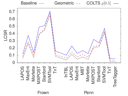
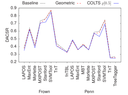
Figure 6: lcsrs and dacsrs for runs without inflations.

Regarding dacsr values, they range from 0.25 for treetagger on penn using adaptive sampling to 0.8788 for svmtool on frown with a geometric schedule. Percentage-wise, 62.75% of those values are greater than 0.4, rising to 64.71% for both arithmetic and geometric runs, while dropping to 58.82% for the adaptive ones, once again showing the adequacy of out experimental setup. Comparing the performances of the three sampling schedules, we see that arithmetic sampling leads in 70.59% of all testing frames and is second best in 23.53%. Next comes the geometric scheduling (resp. colts), outperforming the others 11.76% (resp. 17.65%) of the time and being second in 58.82% (resp. 17.65%) of tests.

In short and as has been noted above, the better approximation to the learning curve given by the baseline (arithmetic scheduling) gives it an advantage in terms of data aquisition costs (dacsrs). Despite this, differences between adaptive (resp. geometric) and baseline runs are very small, with an average of 4.87% (resp. 2.15%), ranging from 0.70% (resp. 0.08%) to 11.50% (resp. 5.65%), and a standard deviation of 3.30% (resp. 1.81%). Once model induction (icsr) is taken into account, colts is shown to perform with the best overall learning costs (lcsrs). However, it is too early to conclude the superiority of the adaptive scheduling over the rest of schema compared. A good selection should also help to identify global rather than local optima, avoiding premature interruptions of the training. In order to explore this ability, we analyze the lcsr and dacsr metrics on the collection $\hat{\mathcal{L}}[1]$ of inflated variants for ${\mathcal{L}}$.

6.3.2 Results on the inflated variants

We now focus on the collection $\hat{\mathcal{L}}[1]$, whose lcsrs (resp. dacsrs) are compiled in the left-hand (resp. right-hand) diagram of Fig. 7. The former range from 0.0156 for tnt on penn with an arithmetic schedule to 0.6522 for svmtool on frown applying colts. In contrast to what happens in ${\mathcal{L}}$, 41.18% of the values are greater than 0.20, which represents a decrease of 1.96% and reveals the impact of the irregularities introduced. Looking into each strategy, results for the arithmetic and geometric ones are the same as those in ${\mathcal{L}}$, at 41.18%. Therefore, the overall decrease associates to adaptive runs, which drop 5.88% to 41.18%. Regarding the best scores, they correspond to our adaptive approach in 88.24% of cases, with the remaining 11.76% favoring the geometric one. At no time does the arithmetic selection lead the results. Geometric scheduling obtains the second best lcsr in 88.24% of trials, followed by the adaptive one with 11.76%. On average, the difference with the baseline is 72.80% for the adaptive runs (from 0.53% to 172.32% with a standard deviation of 72.80%) and 29.95% for the geometric ones (from 0.99% to 76.28% with a standard deviation of 25.65%), while in the arithmetic case it is 9.34% (from 0% to 26.83% with a standard deviation of 6.31%). All this further supports the capacity of colts to adapt to each learning process.

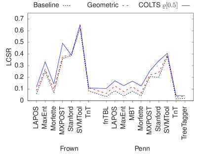
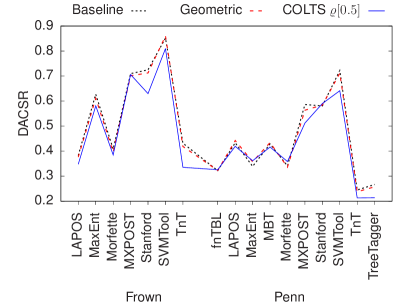
Figure 7: lcsrs and dacsrs for runs with inflations.

Focusing on training resources, dacsrs range from 0.2131 for tnt on penn with an adaptive schedule to 0.8601 for svmtool on frown with a geometric one. Of those values, 58.82% are above 0.40, representing a drop of 3.93% from the experiments in ${\mathcal{L}}$, again due to the irregularities introduced. These losses are not equally shared between all three strategies. While the percentage of arithmetic runs scoring above 0.40 remains the same as in ${\mathcal{L}}$, the one for geometric (resp. adaptive) runs drops 5.89% (resp. 5.89%) to 58.82% (resp. 52.93%). Comparing performances, arithmetic sampling leads in 58.82% of testing frames and is second best in another 23.53%, with geometric (resp. adaptive) sampling besting the others in 17.65% (resp. 23.53%) of cases and running second in another 70.59% (resp. 5.88%). Finally, the difference with the baseline is an average of 9.81% for colts (from 0.34% to 24.12% with an standard deviation of 7.28%), 4.38% for the geometric strategy (from 0.28% to 8.89% with an standard deviation of 2.26%) and 3.30% for the arithmetic one (from 0% to 9.99% with an standard deviation of 2.33%).

In summary, as with the initial local testing frames, inflated arithmetic runs need less training resources (dacsr) than the other ones. But the differences are small enough that, when model induction effort (icsr) is taken into account, colts still comes on top most of the time regarding the overall learning cost (lcsr).

6.3.3 Stability against temporary inflations in performance

The goal is to study the difference between lcsrs (resp. dacsrs) on each run of the local testing frames in the collection ${\mathcal{L}}$ and its corresponding ones in the associated inflated variant of $\hat{\mathcal{L}}[1]$, as shown in the left-hand (resp. right-hand) diagram of Fig. 8. With respect to lcsr values, geometric scheduling leads the results, followed by arithmetic sampling with an average difference for the former (resp. the latter) of 5.48% (resp. 9.34%) and a standard deviation of 6.37% (resp. 6.31%). Adaptive scheduling provides us with the worst average (12.67%) and standard deviation (11.94%).

Results for dacsr are similar. Geometric runs show the best scores, followed by the arithmetic ones with an average difference of 2.42% for the former (resp. 3.30% for the latter) and a standard deviation of 2.88% (resp. 2.33%). colts comes last again, with an average difference of 6.69% and standard deviation of 6.32%, but those differences are even smaller that the ones between lcsr values.

In brief, colts shows a similar degree of stability against inflations to that of the other two selection techniques even, as seen earlier, its overall learning cost (lcsr) is far superior.

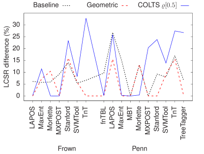
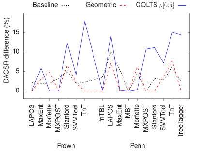
Figure 8: Differences between lcsrs (resp. dacsrs) for runs without and with inflations.

6.3.4 Stability against port variations

Although the above tests support the idea that colts performs better than its opponents, they were obtained from a particular port parameter $\varrho[0.5]$. The question that remains is whether such a conclusion can be generalized, which involves surveying the evolution of performance regarding the port chosen. We then extend the collection of step functions associated to each local testing frame with new adaptive schedules corresponding to port parameters $\varrho[0.2]$ and $\varrho[0.8]$, thereby increasing the number of runs using this kind of scheduling to three. As $\psi\in(0,1]$, $\varrho[0.5]$ is an intermediate value for $\varrho[\psi]$ while the other two are extreme ones, this provides a representative comparative framework on adaptive selection. Focusing on these runs, we now review each local testing frame ${\mathcal{L}}[\mathcal{A}^{\pi}[\mathcal{D}^{\mathcal{K}}_{\Xi_{\eta}}],\wp_{\eta},\tau]\in{\mathcal{L}}$ to study their variations with respect to lcsr (resp. dacsr), as shown in the left-hand (resp. right-hand) diagram of Fig. 9. We also compare them with their corresponding inflated variants in $\hat{\mathcal{L}}[1][\hat{\mathcal{A}}^{\pi}[\mathcal{D}^{\mathcal{K}}_{\Xi_{\eta}}],\wp_{\eta},\tau]\in\hat{\mathcal{L}}[1]$, as seen in Fig. 10.

The new experiments show that lcsr seems to be inversely proportional to the value $\psi$ of $\varrho[\psi]$, reaching the highest (resp. smallest) scores with $\varrho[0.2]$ (resp. $\varrho[0.8]$). The average lcsr for the former (resp. the latter) in ${\mathcal{L}}$ is 0.3015 (resp. 0.2285) with a standard deviation of 0.1820 (resp. 0.1777), while these rates are 0.2621 and 0.1838 for $\varrho[0.5]$, illustrating the reliability of the adaptive technique irrespective of the port used. Regarding stability against irregularities in the working hypotheses, the average difference between the lcsr for runs in ${\mathcal{L}}$ using $\varrho[0.2]$ (resp. $\varrho[0.8]$) as port and their inflated variants in $\hat{\mathcal{L}}[1]$ is 13.04% (resp. 5.49%), with a standard deviation of 17.92% (resp. 7.14%). For $\varrho[0.5]$ the percentages are 12.67% and 11.94% respectively.

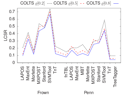
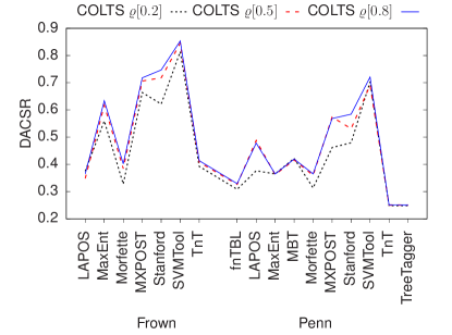
Figure 9: lcsrs and dacsrs for adaptive runs without inflations.

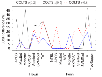
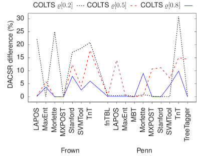
Figure 10: Differences between lcsrs (resp. dacsrs) for adaptive runs without and with inflations.

Regarding training resources (dacsr), model induction savings (icsr) with low $\psi$ values translate into lower efficiency in approximating the real learning curve. Thus, contrary to what has just been shown for lcsrs, dacsr and $\psi$ are directly correlated. So, runs using $\varrho[0.2]$ (resp. $\varrho[0.8]$) have the worst (resp. best) average dacsr of 0.4519 (resp. 0.4980) with a standard deviation of 0.1613 (resp. 0.1789), while runs using $\varrho[0.5]$ represent a middle ground with an average dacsr of 0.4870 and standard deviation of 0.1728. It is worth noticing that the differences between those averages are very small, underlying once again the stability of colts with respect to port. Regarding the effect of irregularities in the learning curve, the average difference between the dacsr for runs in ${\mathcal{L}}$ using $\varrho[0.2]$ (resp. $\varrho[0.8]$) as port and their inflated variants in $\hat{\mathcal{L}}[1]$ is 8.10% (resp. 2.60%), with a standard deviation of 10.90% (resp. 3.45%). For $\varrho[0.5]$ these percentages are 6.69% and 6.32% respectively, matching the behaviour previously observed for lcsr.

Briefly, even the performance is inversely (resp. directly) proportional to the parameter $\psi$ of $\varrho[\psi]$ with respect to overall learning (resp. data acquisition) costs, just as expected and reflected by the lcsr (resp. dacsr) metric, the adaptive scheduling (colts) always maintains acceptable values.

7 Conclusions

We develop an adaptive scheduling (colts) for non-active adaptive sampling in order to reduce the training effort in the generation of ml-based pos taggers. Formally, the technique demonstrates its correctness with respect to its working hypotheses. Namely, it provides the minimal spacing needed between consecutive instances for ensuring that the next observation is relevant in learning terms. Based on a geometrical criterion, the selection task is modeled from a sequence of learning trends which iteratively approximates the learning curve. In every cycle, the algorithm calculates the distance to the next case as the minimal one from where we are sure that the hypothesis of concavity can no longer be guaranteed. The selection schedule described can also be configured according to a port parameter controlling the interaction between the speed of learning and the size of samples. Regarding robustness, our analysis determines that the factors at play are similar to those affecting the stability of the halting condition. Hence, we entrust its treatment to the mechanisms then applied, which first entails having a tool to avoid potentially intractable distortions.

With a view to allow its practical value to be beyond doubt, a demanding and competitive testing framework has been designed for our proposal. Given a learner, a halting condition and a training data base, we categorize schedules according to their performance, seen in terms of both overall learning costs and training resources needed to generate a model with a given level of accuracy. The normalization of the experimental conditions, including a formally correct proximity criterion to measure and stabilize such convergence, ensures that the standards of evidence do not favour any particular option, thus guarantying their reliability.

The results corroborate the expectations established in the theoretical framework as well as its stability. That way, since it does not depend on domain-specific requirements, the doors are open to exploit colts for reducing the workload in ml uses other than the case study considered. The issue is then particularly relevant to tasks in the nlp sphere, where the learning procedures are more and more challenging in a variety of applications such as machine translation, text classification or parsing.

References

- [1] Mohamed Aounallah, Sébastien Quirion, and Guy W. Mineau. Distributed data mining vs. sampling techniques: A comparison. In Advances in Artificial Intelligence, pages 454–460. Springer-Verlag, 2004.
- [2] Josh Attenberg and Foster Provost. Inactive learning? Difficulties employing active learning in practice. ACM SIGKDD Explorations Newsletter, 12(2):36–41, 2011.
- [3] Chris Biemann. Unsupervised part-of-speech tagging employing efficient graph clustering. In Proceedings of the 21st International Conference on Computational Linguistics and 44th Annual Meeting of the Association for Computational Linguistics: Student Research Workshop, pages 7–12, Sydney, 2006.
- [4] Michael Bloodgood and K. Vijay-Shanker. A method for stopping active learning based on stabilizing predictions and the need for user-adjustable stopping. In Proceedings of the 13th Conference on Computational Natural Language Learning, pages 39–47, Boulder, 2009.
- [5] Mary Ann Branch, Thomas F. Coleman, and Yuying Li. A subspace, interior, and conjugate gradient method for large-scale bound-constrained minimization problems. SIAM Journal on Scientific Computing, 21(1):1–23, 1999.
- [6] Thorsten Brants. TnT: A statistical part-of-speech tagger. In Proceedings of the 6th Conference on Applied Natural Language Processing, pages 224–231, Seattle, 2000.
- [7] Eric Brill. Transformation-based error-driven learning and natural language processing: A case study in part-of-speech tagging. Computational Linguistics, 21(4):543–565, 1995.
- [8] George Casella and Roger Berger. Statistical Inference. Duxbury Resource Center, 2001.
- [9] Francisco M. Castro, Manuel J Marín-Jiménez, Nicolás Guil, Cordelia Schmid, and Karteek Alahari. End-to-End Incremental Learning. In Vittorio Ferrari, Martial Hebert, Cristian Sminchisescu, and Yair Weiss, editors, ECCV 2018 - European Conference on Computer Vision, volume 11216 of Lecture Notes in Computer Science, pages 241–257, Munich, Germany, 2018. Springer.
- [10] Jianhua Chen. Properties of a new adaptive sampling method with applications to scalable learning. In Proceedings of the 2013 IEEE/WIC/ACM International Joint Conferences on Web Intelligence (WI) and Intelligent Agent Technologies (IAT) - Volume 01, WI-IAT ’13, pages 9–15, Washington, DC, USA, 2013. IEEE Computer Society.
- [11] H. Chernoff. A measure of asymptotic efficiency for tests of a hypothesis based on the sums of observations. Annals of Mathematical Statistics, 23:409–507, 1952.
- [12] Gzregorz Chrupala, Georgiana Dinu, and Josef van Genabith. Learning morphology with Morfette. In Proceedings of the 6th International Conference on Language Resources and Evaluation, pages 2362–2367, Marrakech, 2008.
- [13] Alexander Clark, Chris Fox, and Shalom Lappin. The Handbook of Computational Linguistics and Natural Language Processing. John Wiley & Sons, Hoboken, 2010.
- [14] David Cohn, Les Atlas, and Richard Ladner. Improving generalization with active learning. Machine Learning, 15(2):201–221, 1994.
- [15] Michael Collins. Discriminative training methods for hidden Markov models: theory and experiments with perceptron algorithms. In Proceedings of the 2002 Conference on Empirical Methods in Natural Language Processing (Vol. 10), pages 1–8, Philadelphia, 2002.
- [16] Walter Daelemans, Jakub Zavrel, Peter Berck, and Steven Gillis. MBT: A memory–based part-of-speech tagger generator. In Proceedings of the 4th Workshop on Very Large Corpora, pages 14–27, Copenhagen, 1996.
- [17] Carlos Domingo, Ricard Gavaldà, and Osamu Watanabe. Adaptive sampling methods for scaling up knowledge discovery algorithms. Data Mining and Knowledge Discovery, 6(2):131–152, 2002.
- [18] Robert M. French. Catastrophic forgetting in connectionist networks. Trends in Cognitive Sciences, 3:128–135, 1999.
- [19] Yoav Freund, H. Sebastian Seung, Eli Shamir, and Naftali Tishby. Selective sampling using the query by committee algorithm. Machine Learning, 28(2-3):133–168, September 1997.
- [20] L.J. Frey and D.H. Fischer. Modeling decision tree performance with the power law. In Proceedings of the 7th International Workshop on Artificial Intelligence and Statistics, pages 59–65, Fort Lauderdale, 1999.
- [21] Johannes Fürnkranz. Integrative windowing. Journal of Artificial Intelligence Research, 8:129–164, 1998.
- [22] E. Giesbrecht and S. Evert. Is part-of-speech tagging a solved task? An evaluation of POS taggers for the German web as corpus. In Proceedings of the 5th Web as Corpus Workshop, pages 27–35, San Sebastian, 2009.
- [23] Jesús Giménez and Lluís Márquez. SVMTool: A general POS tagger generator based on support vector machines. In Proceedings of the 4th International Conference on Language Resources and Evaluation, pages 43–46, Lisbon, 2004.
- [24] Lars Hinrichs, Nicholas Smith, and Birgit Waibel. Manual of information for the part-of-speech-tagged, post-edited ’Brown’ corpora. ICAME Journal, 34:189–233, 2010.
- [25] Wassily Hoeffding. Probability inequalities for sums of bounded random variables. Journal of the American Statistical Association, 58(301):13–30, 1963.
- [26] Ronald A. Howard. Decision analysis: Applied decision theory. In Proceedings of the 4th International Conference on Operational Research, pages 55–71, Cambridge, 1966.
- [27] George John and Pat Langley. Static versus dynamic sampling for data mining. In Proceedings of the 2nd International Conference on Knowledge Discovery and Data Mining, pages 367–370, Portland, 1996.
- [28] C.M. Kadie. Seer: Maximum Likelihood Regression for Learning-Speed Curves. PhD thesis, Univ. of Illinois at Urbana-Champaign, 1995.
- [29] Aloak Kapoor and Russell Greiner. Learning and classifying under hard budgets. In Machine Learning: ECML 2005, pages 170–181. Springer-Verlag, 2005.
- [30] Mark Last. Improving data mining utility with projective sampling. In Proceedings of the 15th ACM SIGKDD International Conference on Knowledge Discovery and Data Mining, pages 487–496, Paris, 2009.
- [31] Rui Leite, Pavel Brazdil, and Joaquin Vanschoren. Selecting classification algorithms with active testing. In Proceedings of the 8th International Conference on Machine Learning and Data Mining in Pattern Recognition, pages 117–131, Berlin, 2012.
- [32] David D. Lewis and William A. Gale. A sequential algorithm for training text classifiers. In Proceedings of the 17th Annual International ACM SIGIR Conference on Research and Development in Information Retrieval, pages 3–12, Dublin, 1994.
- [33] Richard J. Lipton, Jeffrey F. Naughton, Donovan A. Schneider, and S. Seshadri. Efficient sampling strategies for relational database operations. Theoretical Computer Science, 116(1):195 – 226, 1993.
- [34] Viktor Losing, Barbara Hammer, and Heiko Wersing. Incremental on-line learning: A review and comparison of state of the art algorithms. Neurocomputing, 275:1261–1274, 2018.
- [35] James F. Lynch. Analysis and application of adaptive sampling. Journal of Computer and System Sciences, 66(1):2 – 19, 2003. Special Issue on {PODS} 2000.
- [36] Christian Mair and Geoffrey Leech. The Freiburg-Brown corpus (’Frown’) (POS-tagged version). Albert-Ludwigs-Universität Freiburg and University of Lancaster. Available for academic use through http://clu.uni.no/icame/, 2007.
- [37] Mitchell P. Marcus, Beatrice Santorini, Mary Ann Marcinkiewicz, and Ann Taylor. Treebank-3 LDC99T42. Web download file. Linguistic Data Consortium, Philadelphia, 1999.
- [38] Christopher Meek, Bo Thiesson, and David Heckerman. The learning-curve sampling method applied to model-based clustering. The Journal of Machine Learning Research, 2:397–418, March 2002.
- [39] Grace Ngai and Radu Florian. Transformation-based learning in the fast lane. In Proceedings of the 2nd Meeting of the North American chapter of the Association for Computational Linguistics on Language technologies, pages 1–8, Pittsburgh, 2001.
- [40] Foster Provost, David Jensen, and Tim Oates. Efficient progressive sampling. In Proceedings of the 5th ACM SIGKDD International Conference on Knowledge Discovery and Data Mining, pages 23–32, San Diego, 1999.
- [41] John Ross Quinlan. Learning efficient classification procedures and their application to chess end games. In Machine Learning. An Artificial Intelligence Approach, volume 1, pages 463–482, 1983.
- [42] Adwait Ratnaparkhi. A maximum entropy model for part-of-speech tagging. In Proceedings of the 1996 Conference on Empirical Methods in Natural Language Processing, pages 133–142, Philadelphia, 1996.
- [43] Roi Reichart, Omri Abend, and Ari Rappoport. Type level clustering evaluation: New measures and a pos induction case study. In Proceedings of the Fourteenth Conference on Computational Natural Language Learning, CoNLL ’10, pages 77–87, Stroudsburg, PA, USA, 2010. Association for Computational Linguistics.
- [44] Maytal Saar-Tsechansky and Foster Provost. Active sampling for class probability estimation and ranking. Machine Learning, 54(2):153–178, 2004.
- [45] Helmut Schmid. Probabilistic part-of-speech tagging using decision trees. In Proceedings of the International Conference on New Methods in Language Processing, pages 44–49, Manchester, 1994.
- [46] Helmut Schmid and Florian Laws. Estimation of conditional probabilities with decision trees and an application to fine-grained pos tagging. In Proceedings of the 22Nd International Conference on Computational Linguistics - Volume 1, COLING ’08, pages 777–784, Stroudsburg, PA, USA, 2008. Association for Computational Linguistics.
- [47] Hinrich Schütze, Emre Velipasaoglu, and Jan O. Pedersen. Performance thresholding in practical text classification. In Proceedings of the 15th ACM International Conference on Information and Knowledge Management, pages 662–671, Arlington, 2006.
- [48] H. S. Seung, M. Opper, and H. Sompolinsky. Query by committee. In Proceedings of the 5th Annual Workshop on Computational Learning Theory, pages 287–294, Pittsburgh, 1992.
- [49] Hyung-Je Song, Jeong-Woo Son, Tae-Gil Noh, Seong-Bae Park, and Sang-Jo Lee. A cost sensitive part-of-speech tagging: Differentiating serious errors from minor errors. In Proceedings of the 50th Annual Meeting of the Association for Computational Linguistics: Long Papers (Vol. 1), pages 1025–1034, Jeju Island, 2012.
- [50] Katrin Tomanek and Udo Hahn. Approximating learning curves for active-learning-driven annotation. In Proceedings of the 6th International Conference on Language Resources and Evaluation, pages 1319–1324, Marrakech, 2008.
- [51] Kristina Toutanova, Dan Klein, Christopher D. Manning, and Yoram Singer. Feature-rich part-of-speech tagging with a cyclic dependency network. In Proceedings of the 2003 Annual Conference of the North American chapter of the Association for Computational Linguistics on Human Language Technology (Vol. 1), pages 173–180, Edmonton, 2003.
- [52] Cheng-Hao Tsai, Chieh-Yen Lin, and Chih-Jen Lin. Incremental and decremental training for linear classification. Proceedings of the ACM SIGKDD International Conference on Knowledge Discovery and Data Mining, pages 343–352, 2014.
- [53] Yoshimasa Tsuruoka, Yusuke Miyao, and Jun’ichi Kazama. Learning with lookahead: Can history-based models rival globally optimized models? In Proceedings of the 15th Conference on Computational Natural Language Learning, pages 238–246, Portland, 2011.
- [54] Hans van Halteren. Performance of taggers. In Syntactic Wordclass Tagging, pages 81–94. Kluwer Academic Pub., Hingham, 1999.
- [55] Manuel Vilares, Víctor M. Darriba, and Francisco J. Ribadas. Modeling of learning curves with applications to POS tagging. Computer Speech & Language, 41:1–28, 2017.
- [56] Andreas Vlachos. A stopping criterion for active learning. Computer Speech and Language, 22(3):295–312, 2008.
- [57] Osamu Watanabe. Sequential sampling techniques for algorithmic learning theory. Theoretical Computer Science, 348(1):3–14, 2005.
- [58] GaryM. Weiss and Ye Tian. Maximizing classifier utility when there are data acquisition and modeling costs. Data Mining and Knowledge Discovery, 17(2):253–282, 2008.
- [59] P. H. Winston. Learning structural descriptions from examples. In The Psychology of Computer Vision, pages 157–209. McGraw-Hill, New York, 1975.