Abstract

We rigorously derive novel and sharp finite-data error bounds for highly sample-efficient Extended Dynamic Mode Decomposition (EDMD) for both i.i.d. and ergodic sampling. In particular, we show all results in a very general setting removing most of the typically imposed assumptions such that, among others, discrete- and continuous-time stochastic processes as well as nonlinear partial differential equations are contained in the considered system class. Besides showing an exponential rate for i.i.d. sampling, we prove, to the best of our knowledge, the first superlinear convergence rates for ergodic sampling of deterministic systems. We verify sharpness of the derived error bounds by conducting numerical simulations for highly-complex applications from molecular dynamics and chaotic flame propagation.

1 Introduction

Extended Dynamic Mode Decomposition (EDMD; Williams et al. (2015)) is one of the most commonly used machine-learning methods for identifying highly-nonlinear and, in addition, possibly infinite-dimensional dynamical systems from data. At its heart, EDMD provides a data-driven approach to learn the Koopman operator Koopman (1931) propagating observable functions along the flow, which results in a purely data-driven and well-interpretable surrogate model for analysis, prediction, and control, e.g., based on identified symmetries for data augmentation Weissenbacher et al. (2022) or deep learning Han et al. (2021). Since the Koopman operator is a linear, it serves as a powerful tool to leverage well-established concepts from approximation, ergodic, operator, and statistical-learning theory in certifiable machine learning also in safety-critical applications.

Initiated in Mezić (2004; 2005), EDMD and Koopman-based methods have successfully enabled data-driven simulations and analysis of various highly complex applications, such as molecular dynamics Schütte et al. (2016); Wu et al. (2017); Klus et al. (2018), nonlinear partial differential equations including turbulent flows Giannakis et al. (2018); Mezić (2013), quantum mechanics Klus et al. (2022), neuroscience Brunton et al. (2016), deep learning Dogra & Redman (2020), electrocardiography Golany et al. (2021) or climate prediction Azencot et al. (2020) to name just a few. For further applications and Koopman-related learning architectures, we refer to Kutz et al. (2016); Mauroy et al. (2020); Brunton et al. (2022); Retchin et al. (2023).

Convergence of EDMD to the Koopman operator in the infinite data limit was proven in Korda & Mezić (2018). However, despite the enormous success of EDMD, error bounds depending on the number of data samples are still scarce. The first finite-data error bounds were given in Mezić (2022): for deterministic systems based on ergodic sampling under the rather strong assumption that the spectrum of the Koopman operator is discrete and non-dense on the unit circle. First results for i.i.d. (independently and identically distributed) sampling of systems governed by ordinary differential equations (ODEs) can be found in Zhang & Zuazua (2023). For stochastic systems, finite-data error bounds were firstly derived in Nüske et al. (2023) under both i.i.d. and ergodic sampling; including an extension to control systems. However, the result for ergodic sampling hinges on the exponential stability of the Koopman semigroup. For observable functions contained in a Reproducing Kernel Hilbert Space (RKHS), bounds were only recently provided for prediction Philipp et al. (2023a) and control Philipp et al. (2023b) of continuous-time systems, and by Kostic et al. (2023) and Kostic et al. (2022) for i.i.d. sampling from an invariant measure. In conclusion, so far only finite-data error bounds exist for continuous-time systems and, if ergodic sampling is considered, under rather restrictive conditions. Moreover, all bounds decay at most linearly in the amount of data used for estimation.

In this work, we provide a complete analysis of the estimation error of EDMD for a much larger class of Markov processes in Polish spaces. In particular, we remove the (restrictive) requirement of exponential stability and the restriction to systems governed by stochastic differential equations in Nüske et al. (2023). This broadens the class of systems covered by our results such that, in addition, nonlinear partial differential equations and discrete-time Markov processes are included. In particular, all systems considered in Rozwood et al. (2023) are covered rendering the proposed techniques accessible for a sophisticated error analysis w.r.t. the number of used data samples. We provide sharp bounds on the convergence rate and, thus, the sampling efficiency of EDMD, i.e., Koopman-based machine learning for both i.i.d. data and ergodic sampling. Since data can be collected from a single (sufficiently-long) trajectory, which considerably facilitates the data collection process, ergodic sampling is of particular interest for many practical applications as demonstrated in our examples.

Our contribution in this work is three-fold:

1. We severely weaken assumptions made in previous works for ergodic sampling of stochastic systems and prove sharp error bounds with a linear rate.
   

2. We derive the first error bounds showing superlinear convergence for ergodic sampling.
   

3. We establish all our results for continuous- and discrete-time systems – for i.i.d. and ergodic sampling.
   

Notation: We denote the constant function $x\mapsto 1$ by $\mathbbm{1}$. Furthermore, the notation $\langle\cdot,\cdot\rangle_{F}$ and $\|\cdot\|_{F}$ is used for the Frobenius scalar product on $\mathbb{R}^{n\times m}$ and its corresponding norm, respectively. We use the notation $[n:m]:=\mathbb{Z}\cap[n,m]$. For a probability measure $\mu$, the scalar product and the norm on $L^{2}(\mu)$ are denoted by $\langle\cdot,\cdot\rangle$ and $\|\cdot\|$, respectively. The orthogonal projection w.r.t. a closed subspace $M$ in $L^{2}(\mu)$ is denoted by $P_{M}$.

2 EDMD: Data-driven prediction of nonlinear dynamics

Let $(X_{n})_{n\in\mathbb{N}_{0}}$ be a time-homogeneous discrete-time Markov process taking its values in a Polish space $\mathcal{X}$. One representative system class is given by discrete-time dynamical systems

$$x_{n+1}=T(x_{n})+\varepsilon_{n}$$ (DTDS)

with independently and identically distributed (i.i.d.) noise $\varepsilon_{n}$. Another system class contained in our setting are processes, which arise from samples of a time-homogeneous continuous-time Markov process $(Y_{t})_{t\geq 0}$, i.e., $X_{n}=Y_{n\Delta t}$ with sampling period $\Delta t>0$. The process $Y_{t}$ might, e.g., be the solution of a stochastic differential equation

$$dY_{t}=f(Y_{t})\,dt+\sigma(Y_{t})\,dW_{t}.$$ (SDE)

This includes their deterministic analogues, i.e., (DTDS) with $\varepsilon_{n}\equiv 0$ and (SDE) with $\sigma\equiv 0$.

Let $\rho:\mathcal{X}\times\mathfrak{B}(\mathcal{X})\to[0,1]$ denote the transition kernel associated with $(X_{n})$, where $\mathfrak{B}(\mathcal{X})$ denotes the Borel sigma algebra on $\mathcal{X}$, i.e., $\rho(x,A)=\mathbb{P}(X_{n+1}\in A\mid X_{n}=x)$. Then we have $\mathbb{P}^{X_{n+1}}(A)=\int\rho(x,A)\,d\mathbb{P}^{X_{n}}(x)$, where $\mathbb{P}^{X}$ denotes the law of a random variable $X$. Using the notation $\rho_{0}(x,A):=\delta_{x}(A)$ with the Dirac measure $\delta_{x}$, we iteratively define $\rho_{n+1}(x,A):=\int\rho_{n}(y,A)\,\rho(x,dy)$ for $x\in\mathcal{X}$ and $A\in\mathfrak{B}(\mathcal{X})$, where $\rho(x,dy)$ stands for $d\rho(x,\cdot)(y)$. Then, $\rho=\rho_{1}$ and $\mathbb{P}^{X_{n}}(A)=\int\rho_{n}(x,A)\,d\mathbb{P}^{X_{0}}(x)$ hold. For discrete-time deterministic dynamics, i.e., (DTDS) with $\varepsilon_{n}\equiv 0$, we have $\rho(x,A)=\delta_{x}(T^{-1}(A))$.

The Koopman operator and EDMD.

Let $\mu$ be a Borel probability measure on $\mathcal{X}$ satisfying

$$\int\rho(x,A)\,d\mu(x)\,\leq\,L^{2}\mu(A),\qquad A\in\mathfrak{B}(\mathcal{X}),$$ (1)

with a constant $L\geq 0$, see Philipp et al. (2023b) for a detailed discussion. For $p\in[1,\infty)$, the linear, but infinite-dimensional Koopman operator $K_{p}:L^{p}(\mu)\to L^{p}(\mu)$ of the nonlinear process $X_{n}$ is defined by the identity

$$(K_{p}\psi)(x)=\mathbb{E}\big{[}\psi(X_{1})\,|\,X_{0}=x\big{]}=\int\psi(y)\,\rho(x,dy)$$ (2)

for all $\psi\in L^{p}(\mu)$. In the deterministic case (DTDS) with $\varepsilon=0$, this reduces to $K_{p}\psi=\psi\circ T$. An iterative application of (2) yields $(K_{p}^{n}\psi)(x)=\int\psi(y)\,\rho_{n}(x,dy)$ for $n\in\mathbb{N}$. We set $K:=K_{2}$.

Let us briefly recall the well-known extended dynamic mode decomposition (EDMD, see Williams et al. (2015)), which aims at approximating the Koopman operator. To this end, let a dictionary $\mathcal{D}=\{\psi_{1},\ldots,\psi_{N}\}\subset L^{2}(\mu)$ of $\mu$-linearly independent (cf. Definition C.1) continuous functions on $\mathcal{X}$ be given. If we define the $N$-dimensional subspace $\mathbb{V}:=\operatorname{span}\mathcal{D}$ and the matrices $C,C_{+}\in\mathbb{R}^{N\times N}$ by

$$C=\big{(}\langle\psi_{i},\psi_{j}\rangle\big{)}_{i,j=1}^{N}\quad\text{ and }\quad C_{+}=\big{(}\langle\psi_{i},K\psi_{j}\rangle\big{)}_{i,j=1}^{N},$$

then $C$ is invertible, and the matrix representation $K_{\mathbb{V}}$ of the compression $P_{\mathbb{V}}K|_{\mathbb{V}}$ w.r.t. the basis $\mathcal{D}$ is given by

$$K_{\mathbb{V}}=C^{-1}C_{+},$$ (3)

as rigorously shown in Lemma (C.2). In EDMD, the matrix $K_{\mathbb{V}}$ is learned by using evaluations of the dictionary observables on data samples $(x_{k},y_{k})\in\mathcal{X}\times\mathcal{X}$, $k\in[0:m-1]$, which are collected in the $N\times m$ data matrices

$$\Psi_{X}=\big{[}\Psi(x_{k})\big{]}_{k=0}^{m-1}\quad\text{ and }\quad\Psi_{Y}=\big{[}\Psi(y_{k})\big{]}_{k=0}^{m-1},$$

where $\Psi=[\psi_{1},\ldots,\psi_{N}]^{\top}$. Then, the matrix representation of the Koopman operator estimator is given by

$$\widehat{K}_{m}=\widehat{C}^{-1}\widehat{C}_{+},$$ (4)

using the empirical estimators of $C$ and $C_{+}$, respectively, i.e., $\widehat{C}=\tfrac{1}{m}\Psi_{X}\Psi_{X}^{\top}$ and $\widehat{C}_{+}=\tfrac{1}{m}\Psi_{X}\Psi_{Y}^{\top}$.

In this work, we distinguish between two different sampling schemes.

(S1) Ergodic sampling $\mu=\pi$.

We assume the existence of an invariant probability measure $\pi$ for $X_{n}$, i.e.,

$$\int\rho(x,A)\,d\pi(x)=\pi(A),\qquad A\in\mathfrak{B}(\mathcal{X}).$$ (5)

In the deterministic case of (DTDS), invariance of $\pi$ corresponds to $\pi(T^{-1}(A))=\pi(A)$ for all $A\in\mathfrak{B}(\mathcal{X})$, i.e., $T$ is measure-preserving. Further, $\pi$ is assumed to be ergodic, i.e., whenever $A\in\mathfrak{B}(\mathcal{X})$ is such that $\rho(x,A)=1$ for all $x\in A$, then $\pi(A)\in\{0,1\}$.

In this case, the Koopman operator $K_{p}$ is a contraction in $L^{p}(\pi)$ and even an isometry in the deterministic case. The EDMD data consists of samples $x_{k}=X_{k}$ from a single trajectory of $X_{n}$ with $x_{0}\sim\pi$ and $y_{k}=x_{k+1}$. To ensure a.s. invertibility of $\widehat{C}$, we shall assume that for each $(N-1)$-dimensional subspace $M\subset\mathbb{R}^{N}$ and $x\in\Psi^{-1}(M)$, we have $\rho(x,\Psi^{-1}(M))=0$, see Appendix C for a proof of this sufficient condition.

(S2) I.i.d. sampling $\mu=\nu$.

Let $\nu$ be any probability distribution on $\mathcal{X}$ satisfying (1) with some constant $L\geq 0$. In this case, the EDMD data consists of i.i.d. samples $x_{k}\in\mathcal{X}$ and $y_{k}|(x_{k}=x)\sim\rho(x,\,\cdot\,)$. Here, we assure the almost sure invertibility of $\widehat{C}$ by assuming that $m\geq N$ and $\psi_{1},\ldots,\psi_{N}$ are strongly $\mu$-linearly independent, see Appendix C for details including a proof of this characterization.

In the remainder of the manuscript, we tacitly assume

$$\varphi:=\sum_{j=1}^{N}\psi_{j}^{2}\in L^{2}(\mu)$$

in both cases $\mu=\nu$ and $\mu=\pi$ to ensure the existence of the variances of $\widehat{C}_{+}$ and $\widehat{C}$.

3 Certifiable and efficient machine learning

In this section, we provide a concise overview on our main results. In particular, we present novel and sharp error bounds depending on the amount of data samples $m$. The key tool enabling us to derive the error estimates and the respective convergence rates are adroitly-composed formulas to represent the variance, which are shown – together with the in-depth analysis – in the subsequent Section 4.

We motivate our findings by showing numerically approximated convergence rates while referring to Section 5 for a detailed description of the numerical experiments. To be slightly more precise, we consider a reversible stochastic system modeling the folding kinetics of a protein and a deterministic nonlinear partial differential equation given by the Kuramoto-Sivashinsky equation for chaotic flame propagation. In Figure 1, we depict the convergence rate of the learning error $\|K_{\mathbb{V}}-\widehat{K}_{m}\|_{F}$ of EDMD in terms of the amount of data $m$ used for ergodic sampling (S1). We clearly observe that the convergence rate of the error is linear for the molecular dynamics example (note that we depict the root mean square error $[\mathbb{E}[\|\widehat{C}-C\|^{2}_{F}]]^{1/2}$ with corresponding rate $m^{-1/2}$) and superlinear for the deterministic nonlinear partial differential equation (PDE).

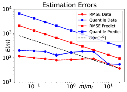
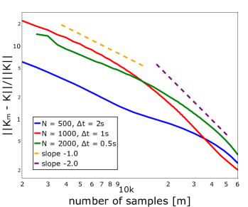
Figure 1: Convergence rate for ergodic sampling of a stochastic system for protein folding (left) and of a deterministic partial differential equation modeling chaotic flame propagation (right).

		Sampling
		i.i.d.$\sim$ probability distribution $\nu$ $\int\rho(x,A)\,\mathrm{d}\nu(x)\leq L^{2}\nu(A)$	invariant and ergodic measure $\pi$ $\int\rho(x,A)\,\mathrm{d}\pi(x)=\pi(A)$
Stochastic	DTDS	✓(Theorem 4.6)	✓(Theorem 4.2)
	SDE	Nüske et al. (2023): ✓	Nüske et al. (2023): exp. stability ✓ (Theorem 4.2)
5
Deterministic	DTDS $(\varepsilon=0)$	✓(Theorem 4.6)	Mezić (2022): linear rate ✓ (Theorem 4.5)	Superlinear rate
	SDE $(\sigma=0)$	Zhang & Zuazua (2023): ✓	✓ (Theorem 4.5)
5

Table 1: Fundamental contributions of this work.

The main contribution are rigorously derived sharp error bounds for data-driven learning in the Koopman framework based on EDMD. As a byproduct, we obtain the first rigorous error analysis directly applicable to a broad class of highly-complex systems, which contains – among many others – the two considered challenging applications. Our key findings are, in addition, summarized in Table 1.

Case (S1): Ergodic sampling of stochastic systems, see Subsection 4.1. For this sampling strategy and the special case (SDE), error bounds with linear rate were already given in Nüske et al. (2023). The proof relied on the assumption that the Koopman semigroup on $\mathbbm{1}^{\perp}$ is exponentially stable. Our first major result Theorem 4.2 does not require this assumption and provides a linear rate for a wide class of stochastic systems, including the molecular dynamics application as well as discrete-time systems like (DTDS). We show that there is a constant $c\geq 0$ such that for all $\varepsilon>0$,

$$\mathbb{P}\big{(}\|K_{\mathbb{V}}-\widehat{K}_{m}\|_{F}>\varepsilon\big{)}\,\leq\,\frac{c}{m\varepsilon^{2}}$$

holds. The corresponding convergence rate depicted in the upper plot of Figure 1 reveals that this linear rate is sharp.

Case (S1): Ergodic sampling of deterministic systems, e.g., (DTDS) with $\varepsilon_{n}\equiv 0$ or (SDE) with $\sigma\equiv 0$, see Subsection 4.2 for details. The main condition for obtaining the above error bound for stochastic systems is that $\lambda=1$ is an isolated eigenvalue of the Koopman operator. Although this assumption is much more general than that of exponential stability of the Koopman semigroup on $\mathbbm{1}^{\perp}$ imposed in Nüske et al. (2023), it excludes a broad class of deterministic cases, cf. Kakutani & Petersen (1981). However, leveraging advanced tools from operator theory, we prove the first superlinear convergence rates for EDMD with ergodic sampling of deterministic systems (such as nonlinear PDEs) as a second major result in Theorem 4.5. That is, we prove that there are constants $c\geq 0$ and $\alpha\geq 1$ such that for all $\varepsilon>0$

$$\mathbb{P}\big{(}\|K_{\mathbb{V}}-\widehat{K}_{m}\|_{F}>\varepsilon\big{)}\leq\frac{c}{m^{\alpha}\varepsilon^{2}}.$$

This rate is observed in the right plot of Figure 1 illustrating EDMD for the Kuramoto-Sivashinsky equation.

Case (S2): i.i.d. sampling of, e.g., (DTDS) or (SDE), see Subsection 4.3 for details. The last major result considers the case of i.i.d. sampling. Going beyond Nüske et al. (2023), and under very general assumptions, we provide an exponential convergence rate for EDMD with i.i.d. sampling using Hoeffding’s inequality in Theorem 4.6. We show that there are constants $c_{1},c_{2}>0$ such that for all $\varepsilon>0$

$$\mathbb{P}\big{(}\|K_{\mathbb{V}}-\widehat{K}_{m}\|_{F}>\varepsilon\big{)}\leq c_{1}\exp(-c_{2}m\varepsilon^{2}).$$

In the upcoming Section 4, we provide the previse statements of the error bounds presented above. Moreover, in Section 5, we revisit the molecular dynamics and flame propagation examples by means of an extensive case study.

4 Sharp convergence rates for EDMD-based machine learning

Our strategy to prove the three estimates presented in Section 3 consists of three major steps. First, we provide a representation formula for the variances of the empirical estimators $\widehat{C}$ and $\widehat{C}_{+}$ in terms of the $m$ sample points. Second, this representation is combined with concentration inequalities, i.e., Markov’s and Hoeffding’s inequality, to deduce a probabilistic bound on the errors $\hat{C}-C$ and $\widehat{C}_{+}-C_{+}$. In a last step, we combine these to a obtain a bound on the learning error $K_{\mathbb{V}}-\widehat{K}_{m}$ in view of (3) and (4).

4.1 Case (S1): Ergodic sampling. Error bounds – almost without assumptions

In this subsection, we let $\mu=\pi$ and draw the data samples from long ergodic trajectories of the process, according to case (S1).

A key step in our error analysis consists of deducing representations of the variances of $\widehat{C}$ and $\widehat{C}_{+}$ which are well-suited for further analysis. For the formulation of our next result, we note that always $K\mathbbm{1}=\mathbbm{1}$, hence, $K\operatorname{span}\{\mathbbm{1}\}\subset\operatorname{span}\{\mathbbm{1}\}$, and also $KL^{2}_{0}(\mu)\subset L^{2}_{0}(\mu)$, where $L^{2}_{0}(\mu)=\operatorname{span}\{\mathbbm{1}\}^{\perp}$. In what follows, we set $K_{0}:=K|_{L^{2}_{0}(\mu)}$, which is a contractive linear operator from $L^{2}_{0}(\mu)$ into itself. Moreover, we define the constants

$$\mathbb{E}_{+}:=\langle K\varphi,\varphi\rangle-\|C_{+}\|_{F}^{2}\qquad\text{and}\qquad\mathbb{E}_{0}:=\|\varphi\|^{2}-\|C\|_{F}^{2}.$$

Theorem 4.1.

(Variance representation) Define the quantities

$$\sigma_{m,+}^{2}:=\mathbb{E}_{+}+\sum_{i,j=1}^{N}\langle p_{m}(K_{0})Qg_{ij},Qg_{ji}^{*}\rangle\qquad\text{and}\qquad\sigma_{m,0}^{2}:=\mathbb{E}_{0}+\sum_{i,j=1}^{N}\langle K_{0}p_{m}(K_{0})Q\psi_{ij},Q\psi_{ij}\rangle,$$

where $\psi_{ij}=\psi_{i}\psi_{j}$, $g_{ij}=\psi_{i}\cdot K\psi_{j}$, $g_{ji}^{*}=\psi_{j}\cdot K^{*}\psi_{i}$, $Q=P_{L^{2}_{0}(\mu)}$, and $p_{m}$ is the polynomial

$$p_{m}(z)=2\sum_{k=1}^{m-1}(1-\tfrac{k}{m})z^{k-1}.$$

Then the variances of $\widehat{C}_{+}$ and $\widehat{C}$ admit the following representations:

$$\mathbb{E}\big{[}\|C_{+}-\widehat{C}_{+}\|_{F}^{2}\big{]}=\frac{\sigma_{m,+}^{2}}{m}\qquad\text{and}\qquad\mathbb{E}\big{[}\|C-\widehat{C}\|_{F}^{2}\big{]}=\frac{\sigma_{m,0}^{2}}{m}.$$

Next, a thorough analysis of the expressions $\sigma_{m,+}^{2}$ and $\sigma_{m,0}^{2}$ in the variance representations leads to the following bounds:

$$\sigma_{m,+}^{2}\leq\left[1+\|p_{m}(K_{0})\|\right]\mathbb{E}_{+}\qquad\text{and}\qquad\sigma_{m,0}^{2}\leq\left[1+\|K_{0}p_{m}(K_{0})\|\right]\mathbb{E}_{0}.$$

So far, the results hold in full generality. However, if we further assume that $\lambda=1$ is an isolated simple eigenvalue of $K$, we may further estimate the above bounds independently of $m$:

$$\begin{split}\sigma_{m,+}^{2}\leq\left[1+4\|(I-K_{0})^{-1}\|\right]\mathbb{E}_{+}\qquad\text{and}\qquad\sigma_{m,0}^{2}\leq\left[1+4\|K_{0}(I-K_{0})^{-1}\|\right]\mathbb{E}_{0}.\end{split}$$ (6)

An application of Markov’s inequality in combination with Lemma C.5 immediately yields the following theorem, which is the main result of this subsection.

Theorem 4.2.

Assume that $\lambda=1$ is an isolated simple eigenvalue of $K$. For $\varepsilon>0$, define the constant

$$\alpha:=\big{[}1+4\|(I-K_{0})^{-1}\|\big{]}\cdot\big{(}2\|C^{-1}\|_{F}\|C_{+}\|_{F}+\varepsilon\big{)}^{2}\cdot\left[\big{(}\|C_{+}\|_{F}^{-2}+\|C^{-1}\|_{F}^{2}\big{)}\|\varphi\|^{2}-2\right].$$

Then we have

$$\mathbb{P}\big{(}\|C^{-1}C_{+}-\widehat{C}^{-1}\widehat{C}_{+}\|_{F}>\varepsilon\big{)}\,\leq\,\frac{\alpha}{m\varepsilon^{2}}.$$

In particular, if $\delta\in(0,1)$, then for $m\geq\frac{\alpha}{\delta\varepsilon^{2}}$ ergodic samples, with probability at least $1-\delta$ we have that $\|C^{-1}C_{+}-\widehat{C}^{-1}\widehat{C}_{+}\|_{F}\leq\varepsilon$.

Remark 4.3.

(a) If $K$ is normal (e.g., self-adjoint or unitary), we have

$$\|(I-K_{0})^{-1}\|=\frac{1}{\operatorname{dist}(1,\sigma(K_{0}))},$$

where $\sigma(K_{0})$ denotes the spectrum of the operator $K_{0}$. If there exist eigenvalues of $K$ close to $\lambda=1$, the above distance is small (hence $\|(I-K_{0})^{-1}\|$ is large) and there exist so-called meta-stable sets, which are almost invariant; that is, trajectories of $X_{n}$ remain in these sets for a long time Davies (1982). In this case, lots of measurements $m$ are needed to gather sufficient information on the process, which is reflected in Theorem 4.2.

(b) If there exist $M\geq 1$ and $\omega>0$ such that $\|K_{0}^{n}\|\leq Me^{-\omega n}$ (which is equivalent to $K_{0}$ having spectral radius smaller than one), then, setting $q=e^{-\omega}<1$, we have

$$\|p_{m}(K_{0})\| =2\Bigg{\|}\sum_{k=1}^{m-1}\tfrac{m-k}{m}\cdot K_{0}^{k-1}\Bigg{\|}\leq 2M\sum_{k=1}^{m-1}\tfrac{m-k}{m}\cdot q^{k-1}=Mp_{m}(q)=\frac{2M}{1-q}\left(1-\frac{1-q^{m}}{m(1-q)}\right)\,\leq\,\frac{2M}{1-q}$$

and $\|K_{0}p_{m}(K_{0})\|\leq\frac{2Mq}{1-q}$. Especially, if $M=1$, we obtain $\sigma_{m,+}^{2}\leq\frac{3-q}{1-q}\cdot\mathbb{E}_{+}$ and $\sigma_{m,0}^{2}\leq\frac{1+q}{1-q}\cdot\mathbb{E}_{0}$. For example, if $K$ is a non-negative self-adjoint operator with an isolated simple eigenvalue at $\lambda=1$, we have $M=1$ and $q=\max\sigma(K_{0})$.

4.2 Case (S1): Ergodic sampling of deterministic systems. Superlinear convergence

Let us consider the deterministic subcase of case (S1), where $K$ is a unitary composition operator with a bijective measure-preserving map $T:\mathcal{X}\to\mathcal{X}$, i.e., $Kf=f\circ T$. The key result is the next theorem, which shows that the variances of $\widehat{C}_{+}$ and $\widehat{C}$ exhibit a direct link to mean ergodicity.

Theorem 4.4.

(Variance representation) Let $K$ be unitary. Then for the variances of $\widehat{C}_{+}$ and $\widehat{C}$, respectively, we have

$$\mathbb{E}\big{[}\|C_{+}-\widehat{C}_{+}\|_{F}^{2}\big{]}=\sum_{i,j=1}^{N}\bigg{\|}\frac{1}{m}\sum_{k=0}^{m-1}K_{0}^{k}Qg_{ij}\bigg{\|}^{2}\qquad\text{and}\qquad\mathbb{E}\big{[}\|C-\widehat{C}\|_{F}^{2}\big{]}=\sum_{i,j=1}^{N}\bigg{\|}\frac{1}{m}\sum_{k=0}^{m-1}K_{0}^{k}Q\psi_{ij}\bigg{\|}^{2}.$$

By the mean ergodic theorem (see, e.g., Krengel (1985)), we know that for every single $f\in L^{2}_{0}(\mu)$ we have that $T_{m}f:=\frac{1}{m}\sum_{k=0}^{m-1}K_{0}^{k}f\to 0$ as $m\to\infty$ (in norm). However, this convergence can be arbitrarily slow and is, in addition, qualitatively bounded from above by $1/m$, which follows from Butzer & Westphal (1971) who proved that $\|T_{m}f\|=o(1/m)$ implies $f=0$. Moreover, it will never be uniform in the sense that $\|T_{m}\|\to 0$ as $m\to\infty$ (see, e.g., Kakutani & Petersen (1981)). We may therefore not assume that $\lambda=1$ is an isolated simple eigenvalue of $K$, since otherwise $T_{m}=\frac{1}{m}(I-K_{0})^{-1}(I-K_{0}^{m})\to 0$ as $m\to\infty$, which is a contradiction.

We therefore have to impose assumptions on the functions that $T_{m}$ is applied to. For a function $f\in L^{2}(\mu)$ we let

$$\mu_{f}(\Delta):=\|E(\Delta)f\|^{2},\quad\Delta\in\mathfrak{B}(\mathbb{T}),$$

where $E$ denotes the spectral measure of the unitary operator $K$, cf. Appendix D. Then $\mu_{f}$ is a finite measure on $\mathbb{T}$ describing the spectral distribution of $f$. Define the finite set of functions

$$\mathcal{F}:=\{Q\psi_{ij}:i,j\in[1:N]\}\,\cup\,\{Qg_{ij}:i,j\in[1:N]\},$$

the arcs $S_{\theta}:=\{e^{it}:-\theta\leq t\leq\theta\}$, $\theta\in(0,\pi)$, and the constant

$$M:=\frac{8(1+\|C^{-1}\|_{F}^{2}\|C_{+}\|_{F}^{2})^{2}}{\|C_{+}\|_{F}^{2}}\cdot\max\{\mathbb{E}_{0},\mathbb{E}_{+}\}.$$

Theorem 4.5.

Assume that $K$ is unitary and suppose that there exist $\alpha\in(1,2)$ and $\kappa\geq 0$ such that for some $\theta\in(0,\pi)$,

$$\mu_{f}(S_{\gamma})\leq\kappa\cdot\mu_{f}(S_{\theta})\cdot(\gamma/\pi)^{\alpha}$$ (7)

for all $f\in\mathcal{F}$ and all $\gamma\in(0,\theta]$. Then for $\varepsilon\in(0,2)$ we have

$$\mathbb{P}\big{(}\|C^{-1}C_{+}-\widehat{C}^{-1} \widehat{C}_{+}\|_{F}>\varepsilon\big{)}\leq\frac{C(\alpha,\kappa,\theta)M}{m^{\alpha}\varepsilon^{2}},$$

where

$$C(\alpha,\kappa,\theta):=2\max\left\{\frac{2}{1-\cos\theta},\frac{3\kappa}{(\alpha-1)(2-\alpha)}\right\}.$$

If $\kappa=0$, then

$$\mathbb{P}\big{(}\|C^{-1}C_{+}-\widehat{C}^{-1} \widehat{C}_{+}\|_{F}>\varepsilon\big{)}\leq\frac{M}{(1-\cos\theta)\cdot m^{2}\varepsilon^{2}}.$$

Let us briefly discuss the condition (7). For this, assume that the spectrum of $K_{0}$ consists of eigenvalues $\lambda_{n}=e^{it_{n}}$ ($t_{n}\searrow 0$) with corresponding eigenfunctions $\varphi_{n}$. Then (7) is equivalent to $\sum_{n:t_{n}\leq\gamma}|\langle f,\varphi_{n}\rangle|^{2}\lesssim\gamma^{\alpha}$. As $\gamma\mapsto\gamma^{\alpha}$ is convex, this allows for relatively large gaps between the eigenvalues in relation to the coefficients $|\langle f,\varphi_{n}\rangle|^{2}$ (in fact, $|\langle f,\varphi_{n}\rangle|^{2}/(t_{n}-t_{n+1})\leq t_{n}^{\alpha-1}$ is sufficient), while a behavior like $\sum_{n:t_{n}<\gamma}|\langle f,\varphi_{n}\rangle|^{2}\sim\gamma^{1/2}$ forces the eigenvalues to be dense at $\lambda=1$. Hence, (7) relates the coefficient decay with the position of the eigenvalues.

4.3 Case (S2): i.i.d. sampling. Bounds on the EDMD estimation error

In this subsection, we let $\mu=\nu$ and draw i.i.d. data samples $(x_{k},y_{k})$ from $d\mu_{0}:=\rho(\cdot,dy)\,d\mu$, according to case (S2). Our main result in this case is the following theorem.

Theorem 4.6.

Assume that $C_{+}\neq 0$. Let $\varepsilon>0$ and set $\sigma=2\|C^{-1}\|_{F}\|C_{+}\|_{F}+\varepsilon$. Then

$$\mathbb{P}\big{(}\|C^{-1}C_{+} -\widehat{C}^{-1}\widehat{C}_{+}\|_{F}>\varepsilon\big{)}\leq\frac{\sigma^{2}}{m\varepsilon^{2}}\left[\big{(}L\|C_{+}\|_{F}^{-2}+\|C^{-1}\|_{F}^{2}\big{)}\|\varphi\|^{2}-2\right].$$

If, in addition, $\varphi\in L^{\infty}(\mu)$, then

$$\mathbb{P}\big{(}\|C^{-1}C_{+}-\widehat{C}^{-1}\widehat{C}_{+}\|_{F}>\varepsilon\big{)}\leq 2\exp\left(-\frac{m\varepsilon^{2}\|C_{+}\|_{F}^{2}}{2\tau^{2}(1+L)^{2}}\right)+2\exp\left(-\frac{m\varepsilon^{2}}{8\tau^{2}\|C^{-1}\|_{F}^{2}}\right),$$

where $\tau=\sigma\|\varphi\|_{\infty}$.

5 Numerical Examples

In this part, we illustrate the deduced error bounds by means of two highly complex examples. The first is a protein folding simulation of a 35-amino acid chain, and the second is a nonlinear chaotic partial differential equation modeling flame propagation.

5.1 Molecular Dynamics Simulation

We apply the Koopman approach to analyze the folding kinetics of the Fip35 WW-domain. This 35-amino acid protein has been used as a benchmarking system in many previous studies due to its small size and fast folding time scale of about ten micro-seconds. We use the $1.1$-milli-second molecular dynamics (MD) simulation data set published by D.E. Shaw research in Lindorff-Larsen et al. (2011). The underlying dynamics are a modified version of Hamiltonian dynamics, defined by a many-body potential energy function $V$ plus a thermostat, which ensures that the position space dynamics are effectively stochastic and reversibly sample the Boltzmann distribution $\exp(-\beta V(x))\,\mathrm{d}x$, enabling estimation of statistical averages via ergodic sampling. The complete data set comprises about $5.6\cdot 10^{6}$ data points.

We build our Koopman model on a 528-dimensional space of inter-atomic distances (closest heavy-atom inter-residue distances), which is a standard featurization for molecular simulation data sets. We employ a basis set of random Fourier features (RFFs) Rahimi & Recht (2007), that is, complex plane waves of the forms

$$\psi_{j}(x)=\exp(i\omega_{j}^{\top}x),$$

where $\omega_{j}$ are frequencies drawn from the spectral measure associated to a Gaussian radial basis function kernel. These features were shown to provide a fairly automatic way of generating an expressive dictionary in Nüske & Klus (2023). The Gaussian bandwidth parameter $\sigma$, the number of random features $p$, and the lag time $t$ for Koopman learning are tuned using the VAMP score metric Wu & Noé (2020), see once again Nüske & Klus (2023) for details. As shown in Figure 2, $\sigma=30$, $p=500$ and $t=1\mu\mathrm{s}$ emerge as suitable parameters to accurately estimate the folding time scale. The leading eigenvectors of the Koopman model can be used to identify the folded and unfolded states from the simulation data, as illustrated in Figure 3. The two leading eigenvectors of the Koopman model are transformed into membership functions $\chi_{0,1}$ by the PCCA method Deuflhard & Weber (2005). A value close to one of these membership functions indicates that the system is in either the folded or unfolded state, as illustrated by representative structures on the left.

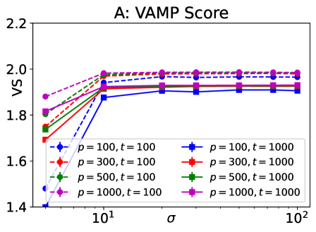
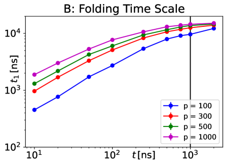
Figure 2: A: VAMP score metric as a function of kernel bandwidth $\sigma$ for different feature sizes $p$ and lag times $t$ (in $\rm[ns]$). Regardless of the lag time, $p=500$ and $\sigma=30$ emerge as optimal. B: Estimated folding timescale for $\sigma=30$ and different feature sizes $p$ as a function of lag time. It can be seen that convergence is achieved for $t=1\,\mu\mathrm{s}$ and $p\geq 500$.

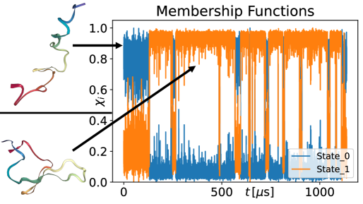
Figure 3: Identification of the folded state of Fip35 based on the Koopman model.

As the MD simulation is reversible, we can apply the error bounds in Eq. (6). Computing the exact asymptotic variances $\sigma_{m,0}^{2}$ and $\sigma_{m,+}^{2}$ via Theorem 4.1 and Eq. (6) requires access to the true eigenvalues and Galerkin matrices $C$, $C_{+}$. Since these are not available, we estimate them by learning a reference model on all available data points. We then compute the error relative to this reference model if the Galerkin matrices are estimated using fewer data points, with $m$ ranging from $m=2000$ to $m=2\cdot 10^{6}$.

In Figure 1 (left), we show the root mean square errors $[\mathbb{E}[\|\widehat{C}-C\|^{2}_{F}]]^{1/2}$ (red) and the 90% error quantile (blue), estimated by our theoretical bounds in Eq. (6) (squares) vs. data-based estimates relative to the reference model (circles) using $50$ different sub-samples of the data set, each of size $m$. Throughout, solid lines refer to $C$, while dashed lines refer to $C_{+}$, but the results are almost indistinguishable. The black line indicates a qualitative decay of the form $cm^{-1/2}$, where the pre-factor $c$ is the average ratio of the data-based RMSE over $m^{-1/2}$, for all values of $m$ greater than the folding time scale. The values of $m$ on the horizontal axis are normalized against the number of data points $m_{f}$ required to reach the folding time scale $10\,\mu\mathrm{s}$. Compared to the theoretical results, the actual error is about an order or magnitude smaller. We notice however, that after an initial period of about the length of the folding time scale, the asymptotic decay of the error is well-described by our estimates (see the black line in the left plot of Figure 1).

5.2 Nonlinear PDE

In our second example, we study the Kuramoto-Sivashinsky equation in two space dimensions, which is a widely-studied deterministic PDE modeling the dynamics of chaotic flame front propagation:

$$\partial_{t}x+\nabla^{2}x+\nabla^{4}x+|\nabla x|^{2}=0.$$ (8)

The system state $x:\Omega\times[0,\infty)\rightarrow\mathbb{R}$ (cf. Figure 4 left) depends on both space and time, and we consider a rectangular domain $\Omega=[-30\pi,30\pi]^{2}$ with periodic boundary conditions.

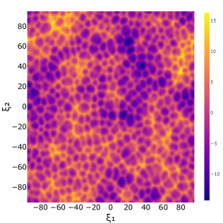
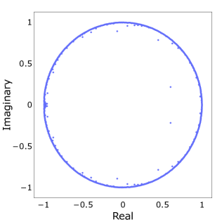
Figure 4: Left: Exemplary snapshot of a state $x(\xi,t)$ on the attractor governed by the Kuramoto-Sivashinsky equation (8). Right: Eigenvalues of the EDMD matrix $\widehat{K}_{M}$

The numerical simulation is realized using the open-source code shenfun Mortensen (2018). For the used domain size, the system exhibits chaotic dynamics, which means that we can use ergodic sampling from a single long trajectory that covers the entire chaotic attractor. In our experiments, we collect a total of $M=100,000$ samples with a time step of $h=0.01$. The spectral element discretization in space yields snapshots of dimension $128\times 128=16,384$, which we reduce to $64\times 64=4,096$ for computational reasons. As this is still prohibitively large for classical dictionaries, we rely on the kernel variant of EDMD Williams et al. (2016). We choose a dictionary $\mathcal{D}$ consisting of $N=1000$ radial basis functions with a twice differentiable Matérn kernel (of order $\nu=2.5$), centered at $N$ spatially equidistant grid points, which means that our Koopman approximation is of dimension $\widehat{K}_{m}\in\mathbb{R}^{N\times N}$. To estimate $\widehat{K}_{m}$ we choose a lag time of $\Delta t=1$, and as we do not have access to the true Koopman compression $K_{\mathbb{V}}$, we study the behavior of the relative error between $\widehat{K}_{m}$ and $\widehat{K}_{M}$ for increasing $m$.

Figure 4 (right) shows the eigenvalue spectrum of the matrix $\widehat{K}_{M}$ for $N=1000$ radial basis functions and all $M$ samples. As usual for chaotic systems (cf. Rowley et al. (2009)) and proven in Subsection 4.2, the eigenvalues are distributed around the unit circle. Consequently, the eigenvalue $\lambda=1$ is not isolated and thus, according to Theorem 4.5, the convergence rate with respect to $m$ should range somewhere between one and two. When taking a closer look at Figure 1 (right), this is exactly the behavior that we observe.

6 Acknowlegdment

We thank D.E. Shaw Research for providing the Fip35 simulation data set.

7 Conclusion

We provided novel sharp error bounds on EDMD for both ergodic and i.i.d. sampling for discrete- and continuous-time nonlinear dynamical systems under rather mild assumptions. For i.i.d. sampling, we established convergence at an exponential rate. Contrary, the convergence of EDMD with ergodic sampling depends on whether the underlying system is stochastic or deterministic. While the error decays at a linear rate in the first case, we show that a broad class of deterministic systems exhibits superlinear convergence. Our theoretical results are underpinned by numerical simulations of highly-complex systems such as the folding kinetics of an acid protein in molecular dynamics and the chaotic nonlinear Kuramoto-Sivashinsky equation. In future research, we investigate suitable choices of the dictionary to speed up the convergence according to the newly identified conditions of Theorem 4.5 in the deterministic case.

Appendix A Proofs of the main results

In this section, we provide proofs for our main theorems. For the convenience of the reader, we repeat the particular results.

A.1 Proof of Theorem 4.2 in Subsection 4.1

In this subsection, we let $\mu=\pi$ be an ergodic and invariant measure for the process $X_{n}$, i.e., case (S1). Furthermore, we assume that for each $(N-1)$-dimensional subspace $M\subset\mathbb{R}^{N}$ and $x\in\Psi^{-1}(M)$ we have $\rho(x,\Psi^{-1}(M))=0$ in order to guarantee the a.s. invertibility of $\widehat{C}$, see Lemma C.4.

Theorem 4.2. Assume that $\lambda=1$ is an isolated simple eigenvalue of $K$. For $\varepsilon>0$, define the constant

$$\alpha:=\big{[}1+4\|(I- K_{0})^{-1}\|\big{]}\cdot\big{[}2\|C^{-1}\|_{F}\|C_{+}\|_{F}+\varepsilon\big{]}^{2}\cdot\left[\big{(}\|C_{+}\|_{F}^{-2}+\|C^{-1}\|_{F}^{2}\big{)}\|\varphi\|^{2}-2\right].$$

Then we have

$$\mathbb{P}\big{(}\|C^{-1}C_{+}-\widehat{C}^{-1}\widehat{C}_{+}\|_{F}>\varepsilon\big{)}\,\leq\,\frac{\alpha}{m\varepsilon^{2}}.$$

In particular, if $\delta\in(0,1)$, then for $m\geq\frac{\alpha}{\delta\varepsilon^{2}}$ ergodic samples, with probability at least $1-\delta$ we have that $\|C^{-1}C_{+}-\widehat{C}^{-1}\widehat{C}_{+}\|_{F}\leq\varepsilon$.

Proof.

In a first step, we provide exact formulae for the variances of $\widehat{C}$ and $\widehat{C}_{+}$ in Theorem 4.1. Next, we find bounds on these variances in Proposition A.1 and apply Markov’s inequality to deduce a probabilistic bound on the errors $\|C_{+}-\widehat{C}_{+}\|_{F}^{2}$ and $\|C-\widehat{C}\|_{F}^{2}$. Then Lemma C.5 immediately yields the desired bound for $\|C^{-1}C_{+}-\widehat{C}^{-1}\widehat{C}_{+}\|^{2}_{F}$. ∎

For completeness, we repeat Theorem 4.1 here. To this end, recall the definitions of $\mathbb{E}_{+}$ and $\mathbb{E}_{0}$:

$$\mathbb{E}_{+}:=\langle K\varphi,\varphi\rangle-\|C_{+}\|_{F}^{2}\qquad\text{and}\qquad\mathbb{E}_{0}:=\|\varphi\|^{2}-\|C\|_{F}^{2}.$$

Theorem 4.1. Define the quantities

$$\sigma_{m,+}^{2}:=\mathbb{E}_{+}+\sum_{i,j=1}^{N}\langle p_{m}(K_{0})Qg_{ij},Qg_{ji}^{*}\rangle\qquad\text{and}\qquad\sigma_{m,0}^{2}:=\mathbb{E}_{0}+\sum_{i,j=1}^{N}\langle K_{0}p_{m}(K_{0})Q\psi_{ij},Q\psi_{ij}\rangle,$$

where $\psi_{ij}=\psi_{i}\psi_{j}$, $g_{ij}=\psi_{i}\cdot K\psi_{j}$, $g_{ji}^{*}=\psi_{j}\cdot K^{*}\psi_{i}$ ($i,j=1,\ldots,N$), $Q=P_{L^{2}_{0}(\mu)}$, and $p_{m}$ is the polynomial

$$p_{m}(z)=2\sum_{k=1}^{m-1}(1-\tfrac{k}{m})z^{k-1}.$$

Then the variances of $\widehat{C}_{+}$ and $\widehat{C}$ admit the following representations:

$$\mathbb{E}\big{[}\|C_{+}-\widehat{C}_{+}\|_{F}^{2}\big{]} =\frac{\sigma_{m,+}^{2}}{m},$$ (9)

$$\mathbb{E}\big{[}\|C-\widehat{C}\|_{F}^{2}\big{]} =\frac{\sigma_{m,0}^{2}}{m}.$$ (10)

Proof.

With $\Phi_{k}:=\Psi(x_{k})\Psi(x_{k+1})^{\top}$, $k=0,\ldots,m-1$, we have

$$\mathbb{E}\big{[}\|C_{+}-\widehat{C}_{+}\|_{F}^{2}\big{]} =\mathbb{E}\bigg{[}\bigg{\|}\frac{1}{m}\sum_{k=0}^{m-1}\big{[}C_{+}-\Phi_{k}\big{]}\bigg{\|}_{F}^{2}\bigg{]}=\frac{1}{m^{2}}\mathbb{E}\bigg{[}\sum_{k=0}^{m-1}\sum_{\ell=0}^{m-1}\big{\langle}C_{+}-\Phi_{k},C_{+}-\Phi_{\ell}\big{\rangle}_{F}\bigg{]}$$

$$=\frac{1}{m^{2}}\mathbb{E}\bigg{[}\sum_{k=0}^{m-1}\big{\|}C_{+}-\Phi_{k}\big{\|}_{F}^{2}+2\sum_{k=1}^{m-1}\sum_{\ell=0}^{k-1}\big{\langle}C_{+}-\Phi_{k},C_{+}-\Phi_{\ell}\big{\rangle}_{F}\bigg{]}$$

$$=\frac{1}{m^{2}}\sum_{k=0}^{m-1}\mathbb{E}\big{[}\|C_{+}-\Phi_{k}\|_{F}^{2}\big{]}+\frac{2}{m^{2}}\sum_{k=1}^{m-1}(m-k)\mathbb{E}\big{[}\big{\langle}C_{+}-\Phi_{k},C_{+}-\Phi_{0}\big{\rangle}_{F}\big{]}$$

$$=\frac{1}{m}\big{(}\mathbb{E}\big{[}\|\Phi_{0}\|_{F}^{2}\big{]}-\|C_{+}\|_{F}^{2}\big{)}+\frac{2}{m}\sum_{k=1}^{m-1}(1-\tfrac{k}{m})\mathbb{E}\big{[}\big{\langle}C_{+}-\Phi_{k},C_{+}-\Phi_{0}\big{\rangle}_{F}\big{]}.$$

Concerning the first summand, we compute

$$\|\Phi_{0}\|_{F}^{2}=\big{\|}\big{(}\psi_{i}(x_{0})\psi_{j}(x_{1})\big{)}_{i,j=1}^{N}\big{\|}_{F}^{2}=\sum_{i,j=1}^{N}\psi_{i}^{2}(x_{0})\psi_{j}^{2}(x_{1})=\varphi(x_{0})\varphi(x_{1})$$ (11)

and hence

$$\mathbb{E}\big{[}\|\Phi_{0}\|_{F}^{2}\big{]}=\int\int\varphi(x)\varphi(y)\,\rho(x,dy)\,d\mu(x)=\int\varphi(x)(K\varphi)(x)\,d\mu(x)=\big{\langle}K\varphi,\varphi\big{\rangle}.$$

Thus,

$$\mathbb{E}\big{[}\|C_{+}-\widehat{C}_{+}\|_{F}^{2}\big{]}=\frac{1}{m}\big{[}\langle K\varphi,\varphi\rangle-\|C_{+}\|_{F}^{2}\big{]}+\frac{2}{m}\sum_{k=1}^{m-1}(1-\tfrac{k}{m})\mathbb{E}\big{[}\big{\langle}C_{+}-\Phi_{k},C_{+}-\Phi_{0}\big{\rangle}_{F}\big{]}.$$

In this case, the cross terms in the second summand do not vanish. First,

$$\mathbb{E}\big{[}\big{\langle}C_{+}-\Phi_{k},C_{+}-\Phi_{0}\big{\rangle}_{F}\big{]}+\|C_{+}\|_{F}^{2} =\mathbb{E}\big{[}\big{\langle}\Phi_{k},\Phi_{0}\big{\rangle}_{F}\big{]}$$

and next,

$$\mathbb{E}\big{[}\big{\langle}\Phi_{k},\Phi_{0}\big{\rangle}_{F}\big{]} =\sum_{i,j=1}^{N}\mathbb{E}\big{[}\psi_{i}(x_{k})\psi_{j}(x_{k+1})\psi_{i}(x_{0})\psi_{j}(x_{1})\big{]}$$

$$=\sum_{i,j=1}^{N}\int\int\int\int\psi_{i}(x^{\prime})\psi_{j}(y^{\prime})\psi_{i}(x)\psi_{j}(y)\,\rho(x^{\prime},dy^{\prime})\,\rho_{k-1}(y,dx^{\prime})\,\rho(x,dy)\,d\mu(x)$$

$$=\sum_{i,j=1}^{N}\int\int\int\psi_{i}(x^{\prime})\psi_{i}(x)\psi_{j}(y)(K\psi_{j})(x^{\prime})\,\rho_{k-1}(y,dx^{\prime})\,\rho(x,dy)\,d\mu(x)$$

$$=\sum_{i,j=1}^{N}\int\int\psi_{i}(x)\psi_{j}(y)\big{(}K^{k-1}g_{ij}\big{)}(y)\,\rho(x,dy)\,d\mu(x)$$

$$=\sum_{i,j=1}^{N}\int\psi_{i}(x)\big{(}K_{1}[\psi_{j}\cdot K^{k-1}g_{ij}]\big{)}(x)\,d\mu(x)$$

$$\overset{(*)}{=}\sum_{i,j=1}^{N}\big{\langle}\psi_{j}\cdot K^{*}\psi_{i},K^{k-1}g_{ij}\big{\rangle}=\sum_{i,j=1}^{N}\big{\langle}g_{ji}^{*},K^{k-1}g_{ij}\big{\rangle}.$$

For a justification of $(*)$ see Lemma B.2 in the Appendix.

Let $P:=P_{\mathbbm{1}}=\langle\,\cdot\,,\mathbbm{1}\rangle\mathbbm{1}$. Then, since $\int g_{ji}^{*}\,d\mu=\int g_{ij}\,d\mu$,

$$\sum_{i,j=1}^{N}\big{\langle}Pg_{ji}^{*},K^{k-1}Pg_{ij}\big{\rangle} =\sum_{i,j=1}^{N}\big{\langle}\langle g_{ji}^{*},\mathbbm{1}\rangle\mathbbm{1},\langle g_{ij},\mathbbm{1}\rangle\mathbbm{1}\big{\rangle}=\sum_{i,j=1}^{N}\left|\int g_{ij}\,d\mu\right|^{2}=\sum_{i,j=1}^{N}|\langle\psi_{i},K\psi_{j}\rangle|^{2}=\|C_{+}\|_{F}^{2}.$$

Similarly, we get

$$\sum_{i,j=1}^{N}\|Pg_{ji}^{*}\|^{2}=\sum_{i,j=1}^{N}\|Pg_{ij}\|^{2}=\|C_{+}\|_{F}^{2}.$$ (12)

Therefore,

$$\mathbb{E}\big{[}\big{\langle}C_{+}-\Phi_{k},C_{+}-\Phi_{0}\big{\rangle}_{F}\big{]}=\sum_{i,j=1}^{N}\big{\langle}K_{0}^{k-1}Qg_{ij},Qg_{ji}^{*}\big{\rangle},$$

and (9) is proved.

The proof of (10) is similar. Here, we set $\widetilde{\Phi}_{k}=\Psi(x_{k})\Psi(x_{k})^{\top}$ and observe that

$$\mathbb{E}\big{[}\|C-\widehat{C}\|_{F}^{2}\big{]}=\frac{1}{m}\big{[}\mathbb{E}[\|\widetilde{\Phi}_{0}\|_{F}^{2}]-\|C_{+}\|_{F}^{2}\big{]}+\frac{2}{m}\sum_{k=1}^{m-1}(1-\tfrac{k}{m})\big{(}\mathbb{E}\big{[}\big{\langle}\widetilde{\Phi}_{k},\widetilde{\Phi}_{0}\big{\rangle}_{F}\big{]}-\|C\|_{F}^{2}\big{)}.$$

Next,

$$\mathbb{E}\big{[}\big{\langle}\widetilde{\Phi}_{k},\widetilde{\Phi}_{0}\big{\rangle}_{F}\big{]} =\sum_{i,j=1}^{N}\mathbb{E}\big{[}\psi_{i}(x_{k})\psi_{j}(x_{k})\psi_{i}(x_{0})\psi_{j}(x_{0})\big{]}=\sum_{i,j=1}^{N}\mathbb{E}\big{[}\psi_{ij}(x_{k})\psi_{ij}(x_{0})\big{]}$$

$$=\sum_{i,j=1}^{N}\int\int\psi_{ij}(x)\psi_{ij}(y)\,\rho_{k}(x,dy)\,d\mu(x)$$

$$=\sum_{i,j=1}^{N}\int\psi_{ij}(x)(K^{k}\psi_{ij})(x)\,d\mu(x)=\sum_{i,j=1}^{N}\big{\langle}K^{k}\psi_{ij},\psi_{ij}\big{\rangle}.$$

In particular, $\mathbb{E}\big{[}\big{\|}\widetilde{\Phi}_{0}\|_{F}^{2}\big{]}=\sum_{i,j=1}^{N}\|\psi_{ij}\|^{2}=\|\varphi\|^{2}$. Finally, making use of

$$\sum_{i,j=1}^{N}\big{\langle}K^{k}P\psi_{ij},P\psi_{ij}\big{\rangle}=\sum_{i,j=1}^{N}\|P\psi_{ij}\|^{2}=\|C\|_{F}^{2},$$ (13)

we obtain (10). ∎

Proposition A.1.

We have

$$\sigma_{m,+}^{2} \leq\left[1+\|p_{m}(K_{0})\|\right]\mathbb{E}_{+}$$

$$\sigma_{m,0}^{2} \leq\left[1+\|K_{0}p_{m}(K_{0})\|\right]\mathbb{E}_{0}.$$

If, in addition, $\lambda=1$ is an isolated simple eigenvalue of $K$, then

$$\sigma_{m,+}^{2} \leq\left[1+4\|(I-K_{0})^{-1}\|\right]\mathbb{E}_{+},$$

$$\sigma_{m,0}^{2} \leq\left[1+4\|K_{0}(I-K_{0})^{-1}\|\right]\mathbb{E}_{0}.$$

Proof.

Let again $P:=P_{\mathbbm{1}}=\langle\,\cdot\,,\mathbbm{1}\rangle\mathbbm{1}$. Then

$$\sum_{i,j=1}^{N}\langle p_{m}(K_{0})Qg_{ij},Qg_{ji}^{*}\rangle \leq\left(\sum_{i,j=1}^{N}\|p_{m}(K_{0})\|^{2}\|Qg_{ij}\|^{2}\right)^{1/2}\left(\sum_{i,j=1}^{N}\|Qg_{ji}^{*}\|^{2}\right)^{1/2}$$

$$=\|p_{m}(K_{0})\|\left(\sum_{i,j=1}^{N}\big{[}\|g_{ij}\|^{2}-\|Pg_{ij}\|^{2}\big{]}\right)^{1/2}\left(\sum_{i,j=1}^{N}\big{[}\|g_{ji}^{*}\|^{2}-\|Pg_{ji}^{*}\|^{2}\big{]}\right)^{1/2}.$$

Now, as $(Kf)^{2}\leq Kf^{2}$ for $f\in L^{4}(\mu)$,

$$\sum_{i,j=1}^{N}\|g_{ij}\|^{2}=\sum_{i,j=1}^{N}\int\psi_{i}^{2}(K\psi_{j})^{2}\,d\mu\,\leq\,\sum_{i,j=1}^{N}\int\psi_{i}^{2}\cdot K\psi_{j}^{2}\,d\mu=\langle K\varphi,\varphi\rangle.$$

Since we also have $(K^{*}f)^{2}\leq K^{*}f^{2}$ for $f\in L^{4}(\mu)$ (cf. Appendix B), we similarly conclude $\sum_{i,j=1}^{N}\|g_{ji}^{*}\|^{2}\leq\langle K\varphi,\varphi\rangle$ and thus (cf. (12))

$$\sum_{i,j=1}^{N}\langle p_{m}(K_{0})Qg_{ij},Qg_{ji}^{*}\rangle\,\leq\,\|p_{m}(K_{0})\|\big{(}\langle K\varphi,\varphi\rangle-\|C_{+}\|_{F}^{2}\big{)}=\|p_{m}(K_{0})\|\cdot\mathbb{E}_{+}.$$

Similarly (cf. (13)),

$$\sum_{i,j=1}^{N}\langle K_{0}p_{m}(K_{0})Q\psi_{ij},Q\psi_{ij}\rangle \leq\|K_{0}p_{m}(K_{0})\|\sum_{i,j=1}^{N}\big{[}\|\psi_{ij}\|^{2}-\|P\psi_{ij}\|^{2}\big{]}=\|K_{0}p_{m}(K_{0})\|\cdot\mathbb{E}_{0}.$$

Assume now that $\lambda=1$ is an isolated simple eigenvalue of $K$. Since

$$p_{m}(z)=\frac{2}{1-z}\bigg{(}1-\frac{1}{m}\sum_{k=0}^{m-1}z^{k}\bigg{)},\qquad z\in\mathbb{C}\backslash\{0\},$$

making use of $\|K_{0}\|\leq 1$, we observe that

$$\|p_{m}(K_{0})\|=\bigg{\|}2(I-K_{0})^{-1}\Big{(}I-\tfrac{1}{m}\sum_{k=0}^{m-1}K_{0}^{k}\Big{)}\bigg{\|}\,\leq\,4\|(I-K_{0})^{-1}\|.$$

Similarly, $\|K_{0}p_{m}(K_{0})\|\leq 4\|K_{0}(I-K_{0})^{-1}\|$. ∎

A.2 Proof of Theorem 4.5 in Subsection 4.2

Let us consider the deterministic subcase of ergodic sampling ,i.e., case (S1), where $K$ is a composition operator with a measure preserving map $T:\mathcal{X}\to\mathcal{X}$. Note that, in this case, we have $K_{1}(fg)=Kf\cdot Kg$ for $f,g\in L^{2}(\mu)$. Let us further assume that $T$ is bijective, so that the corresponding Koopman operator $K$ is unitary. Hence, there exists a bounded self-adjoint operator $A$ on $L^{2}(\mu)$ with $\sigma(A)\subset[-\pi,\pi]$ such that $K=e^{iA}$. We set $A_{0}:=A|_{L^{2}_{0}(\mu)}$.

The following lemma is a slightly extended version of Lemma 4.4.

Lemma 4.4 (Extended version). For the variances of $\widehat{C}_{+}$ and $\widehat{C}$, respectively, we have

$$\begin{split}\mathbb{E}\big{[}\|C_{+}-\widehat{C}_{+}\|_{F}^{2}\big{]}&=\frac{1}{m}\sum_{i,j=1}^{N}\big{\langle}F_{m}(A_{0})Qg_{ij},Qg_{ij}\big{\rangle}=\sum_{i,j=1}^{N}\bigg{\|}\frac{1}{m}\sum_{k=0}^{m-1}K_{0}^{k}Qg_{ij}\bigg{\|}^{2}\end{split}$$ (14)

and

$$\begin{split}\mathbb{E}\big{[}\|C-\widehat{C}\|_{F}^{2}\big{]}&=\frac{1}{m}\sum_{i,j=1}^{N}\big{\langle}F_{m}(A_{0})Q\psi_{ij},Q\psi_{ij}\big{\rangle}=\sum_{i,j=1}^{N}\bigg{\|}\frac{1}{m}\sum_{k=0}^{m-1}K_{0}^{k}Q\psi_{ij}\bigg{\|}^{2},\end{split}$$ (15)

where $F_{m}$ denotes the well known Fejér kernel

$$F_{m}(t)=\sum_{|k|\leq m-1}\big{(}1-\tfrac{|k|}{m}\big{)}e^{ikt}=\frac{1}{m}\left(\frac{1-\cos(mt)}{1-\cos t}\right)^{2}.$$

Proof.

We set $q_{m}(z):=zp_{m}(z)$ and observe that

$$\operatorname{Re}q_{m}(e^{it}) =\sum_{k=1}^{m-1}\big{(}1-\tfrac{k}{m}\big{)}e^{ikt}+\sum_{k=1}^{m-1}\big{(}1-\tfrac{k}{m}\big{)}e^{-ikt}=-1+\sum_{|k|\leq m-1}\big{(}1-\tfrac{|k|}{m}\big{)}e^{ikt}=F_{m}(t)-1.$$

This proves the first equality in (15) as $\sum_{i,j=1}^{N}\|Q\psi_{ij}\|^{2}=\mathbb{E}_{0}$. Let $E$ denote the spectral measure of the unitary operator $K_{0}$. For $\Delta\in\mathfrak{B}(\mathbb{T})$ we compute

$$\langle E(\Delta)Qg_{ij},Qg_{ji}^{*}\rangle =\langle E(\Delta)Qg_{ij},\psi_{j}\cdot K^{*}\psi_{i}\rangle=\langle\psi_{j}\cdot E(\Delta)Qg_{ij},K^{*}\psi_{i}\rangle=\big{\langle}K(\psi_{j}\cdot E(\Delta)Qg_{ij}),\psi_{i}\big{\rangle}$$

$$=\langle K\psi_{j}\cdot KE(\Delta)Qg_{ij},\psi_{i}\rangle=\langle KE(\Delta)Qg_{ij},\psi_{i}\cdot K\psi_{j}\rangle=\langle KE(\Delta)Qg_{ij},Qg_{ij}\rangle,$$

and hence

$$\operatorname{Re}\langle p_{m}(K_{0})Qg_{ij},Qg_{ji}^{*}\rangle =\operatorname{Re}\int p_{m}(\lambda)\,d\langle E_{\lambda}Qg_{ij},Qg_{ji}^{*}\rangle=\operatorname{Re}\int p_{m}(\lambda)\,d\langle K_{0}E_{\lambda}Qg_{ij},Qg_{ij}\rangle$$

$$=\operatorname{Re}\int\lambda p_{m}(\lambda)\,d\langle E_{\lambda}Qg_{ij},Qg_{ij}\rangle=\big{\langle}\operatorname{Re}q_{m}(K_{0})Qg_{ij},Qg_{ij}\big{\rangle}$$

$$=\|Qg_{ij}\|^{2}-\langle F_{m}(A_{0})Qg_{ij},Qg_{ij}\rangle,$$

which yields the first equality in (14). Now, for $f\in L^{2}_{0}(\mu)$ we compute

$$\bigg{\|}\frac{1}{m}\sum_{k=0}^{m-1}K_{0}^{k}f\bigg{\|}^{2}=\frac{1}{m^{2}}\sum_{k,\ell=0}^{m-1}\big{\langle}K_{0}^{k-\ell}f,f\big{\rangle}=\frac{1}{m}\sum_{k=-(m-1)}^{m-1}\frac{m-|k|}{m}\big{\langle}K_{0}^{k}f,f\big{\rangle}=\langle F_{m}(A_{0})f,f\rangle.$$

The lemma is proved. ∎

Remark A.2.

The representation $\big{\|}\frac{1}{m}\sum_{k=0}^{m-1}K_{0}^{k}f\big{\|}^{2}=\langle F_{m}(A_{0})f,f\rangle$ of the square norm of the ergodic series by means of the Fejér kernel is well known, see Kachurovskii & Podvigin (2018).

The main result of this section is the following extended version of Theorem 4.5 which is valid for exponents $\alpha\in(0,2)$. For its formulation, we define

$$C(\alpha)=\begin{cases}\frac{4-3\alpha}{1-\alpha}&\text{for $\alpha\in(0,1)$}\\ 3&\text{for $\alpha=1$}\\ \frac{3}{(\alpha-1)(2-\alpha)}&\text{for $\alpha\in(1,2)$}.\end{cases}$$

and

$$C(\alpha,\kappa,\theta):=2\max\left\{\frac{2}{1-\cos\theta},\kappa C(\alpha)\right\}.$$

Moreover, recall the constant

$$M:=\frac{8(1+\|C^{-1}\|_{F}^{2}\|C_{+}\|_{F}^{2})^{2}}{\|C_{+}\|_{F}^{2}}\cdot\max\{\mathbb{E}_{0},\mathbb{E}_{+}\}.$$

Theorem 4.5. (Extended version) Assume that $K$ is unitary and suppose that there exist $\alpha\in(0,2)$, $\theta\in(0,\pi)$, and $\kappa\geq 0$ such that

$$\mu_{f}(S_{\gamma})\leq\kappa\cdot\mu_{f}(S_{\theta})\cdot(\gamma/\pi)^{\alpha}$$ (16)

for all $f\in\mathcal{F}$ and all $\gamma\in(0,\theta]$. Then for $\varepsilon\in(0,2)$ we have

$$\mathbb{P}\big{(}\|C^{-1}C_{+}-\widehat{C}^{-1}\widehat{C}_{+}\|_{F}>\varepsilon\big{)}\,\leq\,\frac{C(\alpha,\kappa,\theta)M}{m^{\alpha}\varepsilon^{2}}.$$

If $\kappa=0$, then

$$\mathbb{P}\big{(}\|C^{-1}C_{+}-\widehat{C}^{-1} \widehat{C}_{+}\|_{F}>\varepsilon\big{)}\,\leq\,\frac{M}{(1-\cos\theta)\cdot m^{2}\varepsilon^{2}}.$$

Proof.

Theorem 4.5 is proved by combining Lemma C.5 with a result on probabilistic bounds on the errors $\|C_{+}-\widehat{C}_{+}\|_{F}$ and $\|C-\widehat{C}\|_{F}$. These bounds are provided by the Proposition A.3 below. ∎

We set $C_{0}=C$ and $\widehat{C}_{0}=\widehat{C}$.

Proposition A.3.

Let the conditions of the extended version of Theorem 4.5 be satisfied. Then for $\varepsilon>0$ we have

$$\mathbb{P}\big{(}\|C_{i}-\widehat{C}_{i}\|_{F}>\varepsilon\big{)}\,\leq\,\frac{C(\alpha,\kappa,\theta)\cdot\mathbb{E}_{i}}{m^{\alpha}\varepsilon^{2}},\qquad i\in\{+,0\}.$$ (17)

If $\mu_{f}(S_{\theta})=0$ for some $\theta\in(0,\pi)$ and all $f\in\mathcal{F}$, then

$$\mathbb{P}\big{(}\|C_{i}-\widehat{C}_{i}\|_{F}>\varepsilon\big{)}\,\leq\,\frac{2\mathbb{E}_{i}}{(1-\cos\theta)m^{2}\varepsilon^{2}},\qquad i\in\{+,0\}.$$ (18)

Proof.

We prove the statements for $i=0$. Similar reasonings apply to the case $i=+$, respectively.

To show the second statement, assume that there exists $\theta\in(0,\pi)$ such that $\mu_{f}(S_{\theta})=0$ for all $f\in\mathcal{F}$, and let $r(z):=\sum_{k=0}^{m-1}z^{k}$. Then

$$\mathbb{E}\big{[}\|C-\widehat{C}\|_{F}^{2}\big{]} =\sum_{i,j=1}^{N}\bigg{\|}\frac{1}{m}\sum_{k=0}^{m-1}K_{0}^{k}Q\psi_{ij}\bigg{\|}^{2}=\frac{1}{m^{2}}\sum_{i,j=1}^{N}\|r(K_{0})Q\psi_{ij}\|^{2}=\frac{1}{m^{2}}\sum_{i,j=1}^{N}\int_{\mathbb{T}\backslash S_{\theta}}|r(z)|^{2}\,d\mu_{Q\psi_{ij}}(z)$$

$$=\frac{1}{m^{2}}\sum_{i,j=1}^{N}\int_{\mathbb{T}\backslash S_{\theta}}\left|\frac{1-z^{m}}{1-z}\right|^{2}\,d\mu_{Q\psi_{ij}}(z)\,\leq\,\frac{1}{m^{2}}\sum_{i,j=1}^{N}\frac{4}{|1-e^{i\theta}|^{2}}\|Q\psi_{ij}\|^{2}=\frac{2\mathbb{E}_{0}}{(1-\cos\theta)m^{2}}.$$

Hence, (18) follows from Markov’s inequality.

Let us now assume that (16) holds for all $f\in\mathcal{F}$ and all $\gamma\in(0,\theta]$. Let $f=Q\psi_{ij}$ for some fixed pair $i,j\in[1:N]$. Then $f=f_{1}+f_{2}$, where $f_{1}=E(\mathbb{T}\backslash S_{\theta})f$ and $f_{2}=E(S_{\theta})f$. Since $\mu_{f_{1}}(S_{\theta})=0$, we obtain as above that

$$\bigg{\|}\frac{1}{m}\sum_{k=0}^{m-1}K_{0}^{k}f_{1}\bigg{\|}^{2}\,\leq\,\frac{2\|f_{1}\|^{2}}{(1-\cos\theta)m^{2}}.$$

For $f_{2}$ and all $\gamma\in(0,\pi]$ we infer from (16) that

$$\mu_{f_{2}}(S_{\gamma}) =\mu_{f}(S_{\gamma}\cap S_{\theta})=\mu_{f}(S_{\min\{\gamma,\theta\}})\leq\kappa\mu_{f}(S_{\theta})\min\{\gamma,\theta\}^{\alpha}\pi^{-\alpha}$$

$$\leq\kappa\mu_{f}(S_{\theta})(\gamma/\pi)^{\alpha}=\kappa\|E(S_{\theta})f\|^{2}(\gamma/\pi)^{\alpha}=\kappa\|f_{2}\|^{2}(\gamma/\pi)^{\alpha}.$$

Hence, Theorem 2 in Kachurovskii & Podvigin (2018) implies

$$\bigg{\|}\frac{1}{m}\sum_{k=0}^{m-1}K_{0}^{k}f_{2}\bigg{\|}^{2}\,\leq\,\frac{\kappa\|f_{2}\|^{2}C(\alpha)}{m^{\alpha}}.$$

We conclude

$$\bigg{\|}\frac{1}{m}\sum_{k=0}^{m-1}K_{0}^{k}f\bigg{\|}^{2} \leq 2\bigg{\|}\frac{1}{m}\sum_{k=0}^{m-1}K_{0}^{k}f_{1}\bigg{\|}^{2}+2\bigg{\|}\frac{1}{m}\sum_{k=0}^{m-1}K_{0}^{k}f_{2}\bigg{\|}^{2}\,\leq\,\frac{4\|f_{1}\|^{2}}{(1-\cos\theta)m^{2}}+\frac{2\kappa\|f_{2}\|^{2}C(\alpha)}{m^{\alpha}}$$

$$\leq 2\max\left\{\frac{2}{1-\cos\theta},\kappa C(\alpha)\right\}\frac{\|f\|^{2}}{m^{\alpha}}=C(\alpha,\kappa,\theta)\frac{\|f\|^{2}}{m^{\alpha}},$$

and therefore

$$\mathbb{E}\big{[}\|C-\widehat{C}\|_{F}^{2}\big{]} =\sum_{i,j=1}^{N}\bigg{\|}\frac{1}{m}\sum_{k=0}^{m-1}K_{0}^{k}Q\psi_{ij}\bigg{\|}^{2}\leq C(\alpha,\kappa,\theta)\sum_{i,j=1}^{N}\frac{\|Q\psi_{ij}\|^{2}}{m^{\alpha}}=\frac{C(\alpha,\kappa,\theta)\cdot\mathbb{E}_{0}}{m^{\alpha}}.$$

The proposition is proved. ∎

A.3 Proof of Theorem 4.6 in Subsection 4.3

In this subsection, we let $\mu=\nu$ satisfying (1), i.e., we consider the case (S2) of i.i.d. sampling and assume that the observables $\psi_{1},\ldots,\psi_{N}$ are strongly $\mu$-linearly independent, see Definition C.1. Let us recall the main result on the learning error in case (S2) as stated in Theorem 4.6.

Theorem 4.6. Assume that $C_{+}\neq 0$. Let $\varepsilon>0$ and set $\sigma=2\|C^{-1}\|_{F}\|C_{+}\|_{F}+\varepsilon$. Then

$$\mathbb{P}\big{(}\|C^{-1}C_{+} -\widehat{C}^{-1}\widehat{C}_{+}\|_{F}>\varepsilon\big{)}\leq\frac{\sigma^{2}}{m\varepsilon^{2}}\left[\big{(}L\|C_{+}\|_{F}^{-2}+\|C^{-1}\|_{F}^{2}\big{)}\|\varphi\|^{2}-2\right].$$

If, in addition, $\varphi\in L^{\infty}(\mu)$, then

$$\mathbb{P}\big{(}\|C^{-1}C_{+}-\widehat{C}^{-1}\widehat{C}_{+}\|_{F}>\varepsilon\big{)}\leq 2\exp\left(-\frac{m\varepsilon^{2}\|C_{+}\|_{F}^{2}}{2\tau^{2}(1+L)^{2}}\right)+2\exp\left(-\frac{m\varepsilon^{2}}{8\tau^{2}\|C^{-1}\|_{F}^{2}}\right),$$

where $\tau=\sigma\|\varphi\|_{\infty}$.

Proof.

Theorem 4.6 is an immediate consequence of the following Proposition A.4 below, which deduces a probabilistic error bound on $C_{+}-\widehat{C}_{+}$ and $C-\widehat{C}$, and Lemma C.5 which allows to straightforwardly infer the claimed bound on $C^{-1}C_{+}-\widehat{C}^{-1}\widehat{C}_{+}$. ∎

Proposition A.4.

The following probabilistic bounds on the estimation errors hold:

$$\begin{split}\mathbb{P}\big{(}\|C_{+}-\widehat{C}_{+}\|_{F}>\varepsilon\big{)}\leq\frac{\big{\langle}K\varphi,\varphi\big{\rangle}-\|C_{+}\|_{F}^{2}}{m\varepsilon^{2}}\qquad\text{and}\qquad\mathbb{P}\big{(}\|C-\widehat{C}\|_{F}>\varepsilon\big{)}\leq\frac{\|\varphi\|^{2}-\|C\|_{F}^{2}}{m\varepsilon^{2}}.\end{split}$$ (19)

If $\varphi\in L^{\infty}(\mu)$, then

$$\begin{split}\mathbb{P}\big{(}\|C_{+}-\widehat{C}_{+}\|_{F}>\varepsilon\big{)}\leq 2\,e^{-\frac{m\varepsilon^{2}}{2(1+L)^{2}\|\varphi\|_{\infty}^{2}}}\qquad\text{and}\qquad\mathbb{P}\big{(}\|C-\widehat{C}\|_{F}>\varepsilon\big{)}\leq 2\,e^{-\frac{m\varepsilon^{2}}{8\|\varphi\|_{\infty}^{2}}}.\end{split}$$ (20)

Proof.

We set $\Phi_{k}:=\Psi(x_{k})\Psi(y_{k})^{\top}$. As in the proof of Theorem 4.1, we compute

$$\mathbb{E}\big{[}\|C_{+}-\widehat{C}_{+}\|_{F}^{2}\big{]}=\frac{1}{m}\big{[}\langle K\varphi,\varphi\rangle-\|C_{+}\|_{F}^{2}\big{]}+\frac{2}{m}\sum_{k=1}^{m-1}(1-\tfrac{k}{m})\mathbb{E}\big{[}\big{\langle}C_{+}-\Phi_{k},C_{+}-\Phi_{0}\big{\rangle}_{F}\big{]}.$$

The sum $\frac{2}{m}\sum_{k=1}^{m-1}\ldots$ in the last expression vanishes as $\Phi_{k}$ and $\Phi_{0}$ are stochastically independent. Now, apply Markov’s inequality to the non-negative random variable $\|C_{+}-\widehat{C}_{+}\|_{F}^{2}$ to obtain the first probabilistic bound. The second is proved similarly.

Now, assume that $\varphi\in L^{\infty}(\mu)$ and set $S:=\|\varphi\|_{L^{\infty}(\mu)}$. Since $\|K\|\leq L$, we observe that

$$\|C_{+}\|_{F}^{2} =\sum_{i,j=1}^{N}|\langle\psi_{i},K\psi_{j}\rangle|^{2}\leq\sum_{i,j=1}^{N}\|\psi_{i}\|^{2}L^{2}\|\psi_{j}\|^{2}=L^{2}\|\varphi\|_{1}^{2}\leq L^{2}S^{2}.$$

Next, let $(X,Y)\sim\mu_{0}$. Then $\|\Psi(X)\Psi(Y)^{\top}\|_{F}^{2}=\varphi(X)\varphi(Y)$, see (11). We shall prove that $\varphi(X)\varphi(Y)\leq S^{2}$ a.s.. To see this, we note that $X\sim\mu$ and thus $\varphi(X)\leq S$ a.s., so that

$$\mathbb{P}\big{(}\varphi(X)\varphi(Y)>S^{2}\big{)} \leq\mathbb{P}(\varphi(Y)>S)=\mathbb{P}\big{(}(X,Y)\in\mathcal{X}\times\varphi^{-1}((S,\infty))\big{)}$$

$$=\int\rho(x,\varphi^{-1}((S,\infty)))\,d\mu(x)\leq L^{2}\cdot\mu(\varphi^{-1}((S,\infty)))=0.$$

Thus, we obtain that $\|\Psi(x_{k})\Psi(y_{k})^{\top}\|_{F}\leq S$ a.s. for all $k=0,\ldots,m-1$.

Consider the random matrices $D_{k}:=C_{+}-\Psi(x_{k})\Psi(y_{k})^{\top}$, $k=0,\ldots,m-1$. These are stochastically independent, $\mathbb{E}[D_{k}]=0$, and $\|D_{k}\|_{F}\leq(1+L)S$ a.s.. Hence, Hoeffding’s inequality for bounded independent random variables in Hilbert spaces (see Corollary A.5.2 in Mollenhauer (2021) and Theorem 3.5 in Pinelis (1994)) implies that

$$\mathbb{P}\big{(}\|C_{+}-\widehat{C}_{+}\|_{F}>\varepsilon\big{)}=\mathbb{P}\left(\left\|\tfrac{1}{m}\sum_{k=0}^{m-1}D_{k}\right\|_{F}>\varepsilon\right)\,\leq\,2\cdot e^{-\frac{m\varepsilon^{2}}{2(1+L)^{2}S^{2}}},$$

as claimed. The second bound is proved similarly. ∎

Remark A.5.

The bound on $\|C-\widehat{C}\|_{F}$ in Proposition A.4 had been found already in Lemma 3.4.1 of Mollenhauer (2021) (where $\|\varphi\|_{\infty}$ is replaced by the slightly worse constant $N\cdot\max_{i=1,\ldots,N}\|\psi_{i}\|_{\infty}^{2}$).

Appendix B Further aspects of the Koopman operator

The following considers both cases of i.i.d. and ergodic sampling, that is, we let $\mu\in\{\nu,\pi\}$ as in (S1) and (S2).

B.1 Well-definedness of the Koopman operator

Note that (5) and (1) imply $\tau\ll\mu$, where $\tau(A):=\int\rho(x,A)\,d\mu(x)$, with a density $g\in L^{\infty}(\mu)$. In particular, $f\in L^{p}(\mu)$ implies $f\in L^{p}(\tau)$, since $\int|f|^{p}\,d\tau=\int|f|^{p}g\,d\mu\leq\|g\|_{\infty}\int|f|^{p}\,d\mu$.

Note that for every simple function $f$ on $\mathcal{X}$ we have

$$\int f\,d\tau=\int\int f(y)\,\rho(x,dy)\,d\mu(x).$$

Now, let $f\in L^{1}(\mu)$, $f\geq 0$. Then $f\in L^{1}(\tau)$, and there exists a sequence of simple functions $(f_{n})_{n\in\mathbb{N}}$, $0\leq f_{n}\leq f$, such that $f_{n}\uparrow f$ as $n\to\infty$. Hence,

$$\int f\,d\tau=\int(f-f_{n})\,d\tau+\int\int f_{n}(y)\,\rho(x,dy)\,d\mu(x).$$

The first integral approaches zero as $n\to\infty$ by dominated convergence ($0\leq f-f_{n}\leq 2|f|$), and the second integral tends to $\int\int f(y)\,\rho(x,dy)\,d\mu(x)$ as $n\to\infty$ by Beppo-Levi. In particular, $\int f(y)\,\rho(x,dy)<\infty$ for $\mu$-a.e. $x\in\mathcal{X}$, which is the definition of the Koopman operator.

B.2 The adjoint of the Koopman operator

For $f\in L^{1}(\mu)$ define the signed measure

$$\mu_{f}(A):=\int\rho(x,A)f(x)\,d\mu(x),\qquad A\in\mathfrak{B}(\mathcal{X}).$$

If $\mu(A)=0$, then $\int\rho(x,A)\,d\mu(x)\leq L\mu(A)=0$ (where $L=1$ if $\mu=\pi$), hence $\rho(x,A)=0$ for $\mu$-a.e. $x\in\mathcal{X}$, and thus $\mu_{f}(A)=0$. Therefore, there exists a unique $Pf\in L^{1}(\mu)$ such that $\mu_{f}(A)=\int_{A}Pf\,d\mu$ holds for all $A\in\mathfrak{B}(\mathcal{X})$. It is now easily seen that $P:L^{1}(\mu)\to L^{1}(\mu)$ is linear. Moreover, if $f\in L^{1}(\mu)$ and $\Delta_{+}=\{f\geq 0\}$, $\Delta_{-}=\{f<0\}$, we have $\mu_{f}=\mu_{f}^{+}-\mu_{f}^{-}$, where $\mu_{f}^{p}m(A)=\pm\int_{\Delta_{\pm}}\rho(x,A)\,d\mu(x)$, thus

$$\int|Pf|\,d\mu=|\mu_{f}|(\mathcal{X})=\mu_{f}^{+}(\mathcal{X})+\mu_{f}^{-}(\mathcal{X})=\int|f|\,d\mu.$$

Hence, $P$ is an isometry on $L^{1}(\mu)$. It is moreover easy to see that $P$ is a Markov operator, i.e., $P\mathbbm{1}=\mathbbm{1}$ and $Pf\geq 0$ if $f\geq 0$.

For a Borel set $A\in\mathfrak{B}(\mathcal{X})$ and $f\in L^{q}(\mu)$ (where $\frac{1}{p}+\frac{1}{q}=1$) we have

$$\int_{A}K_{p}^{*}f\,d\mu=\langle K_{p}^{*}f,\mathbbm{1}_{A}\rangle_{L^{q},L^{p}}=\langle f,K_{p}\mathbbm{1}_{A}\rangle_{L^{q},L^{p}}=\int\rho(x,A)f(x)\,d\mu(x)=\mu_{f}(A)=\int_{A}Pf\,d\mu.$$

This implies $K_{p}^{*}f=Pf$. In particular, $P$ maps $L^{q}(\mu)$ into $L^{q}(\mu)$ for all $q\in[1,\infty]$ and coicides there with $K_{p}^{*}$ for $q\neq 1$.

Lemma B.1.

For $f\in L^{2}(\mu)$ we have $(Pf)^{2}\leq Pf^{2}$ $\mu$-a.e.

Proof.

Let $f$ be a simple function, i.e., $f=\sum_{i=1}^{n}a_{i}\mathbbm{1}_{A_{i}}$, where the $A_{i}$ are mutually disjoint and $\bigcup_{i=1}^{n}A_{i}=\mathcal{X}$. Then $\sum_{i=1}^{n}P\mathbbm{1}_{A_{i}}=P\mathbbm{1}=\mathbbm{1}$, hence, by convexity of $z\mapsto z^{2}$,

$$(Pf)^{2}(x)=\Big{(}\sum_{i=1}^{n}a_{i}(P\mathbbm{1}_{A_{i}})(x)\Big{)}^{2}\,\leq\,\sum_{i=1}^{n}a_{i}^{2}(P\mathbbm{1}_{A_{i}})(x)=(Pf^{2})(x)$$

and therefore $(Pf)^{2}\leq Pf^{2}$. Similarly, $|Pf|\leq P|f|$. If $f\in L^{2}(\mu)$, let $(f_{n})$ be a sequence of simple functions such that $\|f_{n}-f\|_{L^{2}(\mu)}\to 0$ as $n\to\infty$. Then, for every $A\in\mathfrak{B}(\mathcal{X})$,

$$\int_{A}\big{[}(Pf)^{2}-Pf^{2}\big{]}\,d\mu \leq\int_{A}((Pf)^{2}-(Pf_{n})^{2})\,d\mu+\int_{A}(Pf_{n}^{2}-Pf^{2})\,d\mu$$

$$\leq\int|P(f-f_{n})P(f+f_{n})|\,d\mu+\|P(f_{n}^{2}-f^{2})\|_{L^{1}(\mu)}$$

$$\leq\|P(f_{n}-f)\|_{L^{2}(\mu)}\|P(f_{n}+f)\|_{L^{2}(\mu)}+\|f_{n}^{2}-f^{2}\|_{L^{1}(\mu)}$$

$$\leq 2\|f_{n}-f\|_{L^{2}(\mu)}\|f_{n}+f\|_{L^{2}(\mu)}.$$

This proves $(Pf)^{2}\leq Pf^{2}$ $\mu$-a.e. for all $f\in L^{2}(\mu)$. ∎

Lemma B.2.

Let $f,g,h\in L^{2}(\mu)$ such that $g^{2}Pf^{2}\in L^{1}(\mu)$. Then $f\cdot K_{1}(gh)\in L^{1}(\mu)$ and

$$\int f\cdot K_{1}(gh)\,d\mu=\int[g\cdot K^{*}f]\cdot h\,d\mu.$$

Proof.

Let $(f_{n})\subset L^{\infty}(\mu)$ be a sequence of simple functions such that $f_{n}\to f$ and $|f_{n}|\nearrow|f|$ pointwise $\mu$-a.e. as $n\to\infty$. Then

$$\int|K^{*}(f_{n}-f)|\,d\mu\,\leq\,\int K^{*}|f_{n}-f|\,d\mu=\int|f_{n}-f|\,d\mu,$$

which converges to zero as $n\to\infty$ by dominated convergence ($|f_{n}-f|\leq 2|f|$). Hence, there exists a subsequence $(f_{n_{k}})$ such that $K^{*}f_{n_{k}}\to K^{*}f$ $\mu$-a.e. as $k\to\infty$. WLOG, we may therefore assume that $K^{*}f_{n}\to K^{*}f$ $\mu$-a.e. as $n\to\infty$. By monotone convergence,

$$\int|f||K_{1}(gh)|\,d\mu =\lim_{n\to\infty}\int|f_{n}||K_{1}(gh)|\,d\mu\leq\limsup_{n\to\infty}\int|f_{n}|\cdot K_{1}(|gh|)\,d\mu$$

$$=\limsup_{n\to\infty}\int K_{1}^{*}|f_{n}|\cdot|gh|\,d\mu\,\leq\,\int|g|P|f|\cdot|h|\,d\mu,$$

which is a finite number. Hence, indeed, $f\cdot K_{1}(gh)\in L^{1}(\mu)$ and, by dominated convergence,

$$\int f\cdot K_{1}(gh)\,d\mu =\lim_{n\to\infty}\int f_{n}\cdot K_{1}(gh)\,d\mu=\lim_{n\to\infty}\int[g\cdot K_{1}^{*}f_{n}]\cdot h\,d\mu=\int[g\cdot K^{*}f]\cdot h\,d\mu,$$

as claimed. ∎

Appendix C Auxiliary results

In this section, we provide auxiliary results on the invertibility of the considered matrices.

Definition C.1.

Let $\mu$ be an arbitrary measure on $\mathcal{X}$, and let measurable functions $\psi_{1},\ldots,\psi_{N}:\mathcal{X}\to\mathbb{R}$ be given.

(a) We say that $\psi_{1},\ldots,\psi_{N}$ are linearly independent w.r.t. the measure $\mu$ (or simply $\mu$-linearly independent) if $\sum_{j=1}^{N}\lambda_{j}\psi_{j}=0$ $\mu$-a.e. implies $\lambda_{1}=\dots=\lambda_{N}=0$.

(b) We say that $\psi_{1},\ldots,\Psi_{N}$ are strongly linearly independent w.r.t. the measure $\mu$ (or simply strongly $\mu$-linearly independent) if $\mu\left(\sum_{j=1}^{N}\lambda_{j}\psi_{j}=0\right)>0$ implies $\lambda_{1}=\dots=\lambda_{N}=0$.

If $\psi_{1},\ldots,\Psi_{N}$ are strongly $\mu$-linearly independent, it follows in particular that the sets of zeros $\psi_{j}^{-1}(\{0\})$ are null sets (w.r.t. $\mu$). Furthermore, note that the following implications hold:

strong $\mu$-linear independence$\quad\Longrightarrow\quad$ $\mu$-linear independence$\quad\Longrightarrow\quad$linear independence.

The following lemma holds for both cases (S1) and (S2).

Lemma C.2.

Let $\mu\in\{\nu,\pi\}$ and let $\psi_{1},\ldots,\psi_{N}$ be $\mu$-linearly independent. Then, the matrix $C$ is invertible, and the matrix representation $\widetilde{K}_{\mathbb{V}}$ of the compression $P_{\mathbb{V}}K|_{\mathbb{V}}$ of $K$ to $\mathbb{V}$ is given by $\widetilde{K}_{\mathbb{V}}=C^{-1}C_{+}$.

Proof.

Let $v\in\mathbb{R}^{N}$ such that $Cv=0$. Then we have $\sum_{j=1}^{N}\langle\psi_{i},\psi_{j}\rangle v_{j}=0$ and hence $\langle\psi_{i},\sum_{j=1}^{N}v_{j}\psi_{j}\rangle=0$ for all $i\in[N]$. But this implies $\sum_{j=1}^{N}v_{j}\psi_{j}=0$ $\mu$-a.e. and thus $v_{1}=\cdots=v_{N}=0$ as the $\psi_{j}$ are $\mu$-linearly independent. Hence, $C$ is indeed invertible.

For any $j\in[N]$, we have $P_{\mathbb{V}}K\psi_{j}=\sum_{i=1}^{N}a_{ij}\psi_{i}$ with some $a_{ij}\in\mathbb{R}$ forming the matrix $\widetilde{K}_{\mathbb{V}}=(a_{ij})_{i,j=1}^{N}$. Next, for $i,j\in[N]$,

$$(C_{+})_{ij}=\langle\psi_{i},K\psi_{j}\rangle=\langle\psi_{i},P_{\mathbb{V}}K\psi_{j}\rangle=\Big{\langle}\psi_{i},\sum_{\ell=1}^{N}a_{\ell j}\psi_{\ell}\Big{\rangle}=\sum_{\ell=1}^{N}\langle\psi_{i},\psi_{\ell}\rangle a_{\ell j}=(C\widetilde{K}_{\mathbb{V}})_{ij},$$

and the claim follows. ∎

Lemma C.3.

In case (S2), $\widehat{C}$ is invertible a.s. if and only if $m\geq N$ and $\psi_{1},\ldots,\psi_{N}$ are strongly $\mu$-linearly independent.

Proof.

First of all, note that $\widehat{C}$ is invertible if and only if the rank of $\Psi_{X}$ equals $N$.

Assume that the $\psi_{j}$ are strongly linearly independent and $m\geq N$. Define the random variables $Y_{j}:=\Psi(x_{j})\in\mathbb{R}^{N}$, $j=0,\ldots,m-1$, and the pushforward measure $\tau:=\mu\circ\Psi^{-1}$. Then the $Y_{j}$ are $\tau$-distributed and independent, and we have $\mathbb{P}(\lambda^{\top}Y_{j}=0)=0$ for all $j$ and all $\lambda\in\mathbb{R}^{N}\backslash\{0\}$.

We shall show that $Y_{0},\ldots,Y_{N-1}$ are linearly independent a.s. For this, fix $j\in\{0,\ldots,N-1\}$, let $J\subset\{0,\ldots,N-1\}\backslash\{j\}$ with $1\leq k\leq N-1$ elements, and define

$$V:=\big{\{}(y_{1},\ldots,y_{k+1})\in(\mathbb{R}^{N})^{k+1}:y_{k+1}\in\operatorname{span}\{y_{1},\ldots,y_{k}\}\big{\}}.$$

Then we have

$$\mathbb{P}\big{(}Y_{j}\in\operatorname{span}\{Y_{i}:i\in J\}\big{)} =\tau^{k+1}(V)=\int_{(\mathbb{R}^{N})^{k}}\int_{\operatorname{span}\{y_{1},\ldots,y_{k}\}}\,d\tau(y)\,d\tau^{k}(y_{1},\ldots,y_{k})$$

$$=\int_{(\mathbb{R}^{N})^{k}}\mathbb{P}\big{(}Y_{j}\in\operatorname{span}\{y_{1},\ldots,y_{k}\}\big{)}\,d\tau^{k}(y_{1},\ldots,y_{k}).$$

Fix $k$ vectors $y_{1},\ldots,y_{k}\in\mathbb{R}^{N}$. Then there exists $\lambda\in\mathbb{R}^{N}\backslash\{0\}$ such that $\lambda^{\top}[y_{1},\ldots,y_{k}]=0$, hence

$$\mathbb{P}\big{(}Y_{j}\in\operatorname{span}\{y_{1},\ldots,y_{k}\}\big{)}\leq\mathbb{P}(\lambda^{\top}Y_{j}=0)=0.$$

This implies $\mathbb{P}\big{(}Y_{j}\in\operatorname{span}\{Y_{i}:i\in J\}\big{)}=0$, which proves the claim.

Conversely, assume that $\Psi_{X}$ has rank $N$ a.s., let $\lambda\in\mathbb{R}^{N}\backslash\{0\}$ and set $Z:=\{\lambda^{\top}\Psi=0\}\subset\mathcal{X}$. Then

$$0=\mathbb{P}(\lambda^{\top}\Psi_{X}=0)=\mathbb{P}(x_{k}\in Z\;\forall k=0,\ldots,m-1)=\mu^{m}(Z^{m})=[\mu(Z)]^{m},$$

which proves that $\psi_{1},\ldots,\psi_{N}$ are strongly $\mu$-linearly independent. ∎

Lemma C.4.

Let $m\geq N+1$. In case (S1), $\widehat{C}$ is invertible a.s. if for each $(N-1)$-dimensional subspace $M\subset\mathbb{R}^{N}$ and $x\in\Psi^{-1}(M)$ we have $\rho(x,\Psi^{-1}(M))=0$.

Proof.

If $\mathcal{L}\subset\mathbb{R}^{N}$ is a subspace with $\dim\mathcal{L}<N-1$, for any $x\in\mathcal{X}$ there exists an $(N-1)$-dimensional subspace $M\supset\mathcal{L}$ with $x\in\Psi^{-1}(M)$, and we obtain $\rho(x,\Psi^{-1}(\mathcal{L}))\leq\rho(x,\Psi^{-1}(M))=0$. Hence, the assumption holds for all subspaces $M\subset\mathbb{R}^{N}$.

In the following, let $A:=\Psi^{-1}(\{0\})$. Assume that $\mu(A)>0$. Note that $\mu(A)<1$ by $\mu$-linear independence of the $\psi_{j}$. We show that

$$\mathbb{P}([\Psi(X_{1}),\ldots,\Psi(X_{N})]\text{ invertible}\,|\,X_{0}\in A) =1$$ (21)

$$\mathbb{P}([\Psi(X_{0}),\ldots,\Psi(X_{N-1})]\text{ invertible}\,|\,X_{0}\notin A) =1.$$ (22)

Then the claim follows. By assumption, we have $\rho(x,A)=0$ for $x\in A$, hence

$$\mathbb{P}(\Psi(X_{1})=0\,|\,X_{0}\in A)=\frac{1}{\mu(A)}\int_{A}\rho(x,A)\,d\mu(x)=0$$

Next, let $k\in\{1,\ldots,N-1\}$ and set $M(x_{1},\ldots,x_{k}):=\operatorname{span}\{\Psi(x_{1}),\ldots,\Psi(x_{k})\}$ for $x_{1},\ldots,x_{k}\in\mathcal{X}$. Then

$$\mathbb{P}\big{(}\Psi(X_{k+1}) \in M(X_{1},\ldots,X_{k})\,|\,X_{0}\in A\big{)}$$

$$=\frac{1}{\mu(A)}\int_{A}\int_{x_{1}}\dots\int_{x_{k}}\int_{\Psi^{-1}(M(x_{1},\ldots,x_{k}))}\rho(x_{k},dx_{k+1})\rho(x_{k-1},dx_{k})\dots\rho(x_{0},dx_{1})\,d\mu(x_{0})$$

$$=\frac{1}{\mu(A)}\int_{A}\int_{x_{1}}\dots\int_{x_{k}}\rho(x_{k},\Psi^{-1}(M(x_{1},\ldots,x_{k})))\rho(x_{k-1},dx_{k})\dots\rho(x_{0},dx_{1})\,d\mu(x_{0}).$$

Now, note that for all $x_{k}\in\mathcal{X}$ we have $x_{k}\in\Psi^{-1}(M(x_{1},\ldots,x_{k}))$, hence $\rho(x_{k},\Psi^{-1}(M(x_{1},\ldots,x_{k})))=0$. Therefore, we have $\mathbb{P}\big{(}\Psi(X_{k+1})\in M(X_{1},\ldots,X_{k})\,|\,X_{0}\in A\big{)}=0$ for all $k=1,\ldots,N-1$, which shows (21). The relation (22) can be shown similarly with all indices dropped by one and $A$ replaced by $\mathcal{X}\backslash A$. The proof for (22) carries over to the case $\mu(A)=0$ without conditioning and with $\mathcal{X}\setminus A$ replaced by $\mathcal{X}$. ∎

The following result provides an improved version of Theorem 12 in Nüske et al. (2023).

Lemma C.5.

Let $C,D\in\mathbb{R}^{N\times N}$ be such that $C$ is invertible and $D\neq 0$. Let $\widehat{C},\widehat{D}\in\mathbb{R}^{N\times N}$ be random matrices such that $\widehat{C}$ is invertible a.s.. Then for any sub-multiplicative matrix norm $\|\,\cdot\,\|$ on $\mathbb{R}^{N\times N}$ and any $\varepsilon>0$ we have

$$\mathbb{P}\big{(}\|C^{-1}D-\widehat{C}^{-1}\widehat{D}\|>\varepsilon\big{)}\leq\mathbb{P}\Big{(}\|D-\widehat{D}\|>\tfrac{\varepsilon}{\tau}\|D\|\Big{)}+\mathbb{P}\Big{(}\|C-\widehat{C}\|>\tfrac{\varepsilon}{\tau}\|C^{-1}\|^{-1}\Big{)},$$

where $\tau=2\|C^{-1}\|\|D\|+\varepsilon$.

Proof.

We have $C^{-1}D-\widehat{C}^{-1}\widehat{D}=\widehat{C}^{-1}(D-\widehat{D})+(C^{-1}-\widehat{C}^{-1})D$ and thus

$$\mathbb{P}\big{(}\|C^{-1}D-\widehat{C}^{-1}\widehat{D}\|>\varepsilon\big{)} \leq\mathbb{P}\big{(}\|\widehat{C}^{-1}\|\|D-\widehat{D}\|+\|D\|\|C^{-1}-\widehat{C}^{-1}\|>\varepsilon\big{)}$$

$$\leq\mathbb{P}\big{(}\|\widehat{C}^{-1}\|\|D-\widehat{D}\|>\tfrac{\varepsilon}{2}\;\vee\;\|D\|\|C^{-1}-\widehat{C}^{-1}\|>\tfrac{\varepsilon}{2}\big{)}$$

$$=\mathbb{P}\Big{(}\|D-\widehat{D}\|>\tfrac{\varepsilon/2}{\|\widehat{C}^{-1}\|}\;\vee\;\|C^{-1}-\widehat{C}^{-1}\|>\tfrac{\varepsilon/2}{\|D\|}\Big{)}$$

$$\leq\mathbb{P}\Big{(}\|D-\widehat{D}\|>\tfrac{\varepsilon/2}{\|C^{-1}\|+\tfrac{\varepsilon/2}{\|D\|}}\;\vee\;\|C^{-1}-\widehat{C}^{-1}\|>\tfrac{\varepsilon/2}{\|D\|}\Big{)}$$

$$\leq\mathbb{P}\Big{(}\|D-\widehat{D}\|>\tfrac{\varepsilon/2}{\tau}\|D\|\Big{)}+\mathbb{P}\Big{(}\|C^{-1}-\widehat{C}^{-1}\|>\tfrac{\varepsilon/2}{\|D\|}\Big{)}.$$

Next, we estimate

$$\|C^{-1}-\widehat{C}^{-1}\|=\|C^{-1}(\widehat{C}-C)\widehat{C}^{-1}\|\,\leq\,\|C^{-1}\|\|\widehat{C}-C\|\big{(}\|\widehat{C}^{-1}-C^{-1}\|+\|C^{-1}\|\big{)}.$$

Hence, if $\|C-\widehat{C}\|<\frac{1}{\|C^{-1}\|}$, then

$$\|C^{-1}-\widehat{C}^{-1}\|\,\leq\,\frac{\|C^{-1}\|^{2}\|C-\widehat{C}\|}{1-\|C^{-1}\|\|C-\widehat{C}\|}$$

Therefore,

$$\mathbb{P}\Big{(}\|C^{-1}-\widehat{C}^{-1}\|>\tfrac{\varepsilon/2}{\|D\|}\Big{)} \leq\mathbb{P}\Big{(}\|C-\widehat{C}\|\geq\tfrac{1}{\|C^{-1}\|}\;\vee\;\tfrac{\|C^{-1}\|^{2}\|C-\widehat{C}\|}{1-\|C^{-1}\|\|C-\widehat{C}\|}>\tfrac{\varepsilon/2}{\|D\|}\Big{)}$$

$$=\mathbb{P}\Big{(}\|C-\widehat{C}\|\geq\tfrac{1}{\|C^{-1}\|}\;\vee\;\|C-\widehat{C}\|>\tfrac{\varepsilon/2}{\|C^{-1}\|(\|D\|\|C^{-1}\|+\varepsilon/2)}\Big{)}$$

$$=\mathbb{P}\Big{(}\|C-\widehat{C}\|>\tfrac{\varepsilon/2}{\|C^{-1}\|(\|D\|\|C^{-1}\|+\varepsilon/2)}\Big{)},$$

and the lemma is proved. ∎

Appendix D Spectral measures of unitary operators

Let $U$ be a unitary operator in a Hilbert space $\mathcal{H}$. By the spectral theorem for normal operators in Hilbert spaces (see, e.g., Conway (2010)), there exists an operator-valued measure $E$ on the Borel sigma algebra $\mathcal{B}$ of $\mathbb{T}=\{z\in\mathbb{C}:|z|=1\}$, which has the following properties:

• $E(\Delta)$ is an orthogonal projection for all $\Delta\in\mathfrak{B}$.

• $E(\mathbb{T}\backslash\sigma(U))=0$ and $E(\sigma(U))=I$.

• $E(\Delta_{1}\cap\Delta_{2})=E(\Delta_{1})E(\Delta_{2})=E(\Delta_{2})E(\Delta_{1})$ for $\Delta_{1},\Delta_{2}\in\mathcal{B}$.

• $E(\Delta)\mathcal{H}$ is $U$-invariant for each $\Delta\in\mathcal{B}$.

• $\sigma(U|_{E(\Delta)\mathcal{H}})\subset\sigma(U)\cap\Delta$ for closed $\Delta\in\mathcal{B}$.

The measure $E$ is called the spectral measure of $U$. In the finite-dimensional case (i.e., when $U\in\mathbb{C}^{n\times n}$ is a unitary matrix), the projection $E(\Delta)$ is the orthogonal projection onto the sum of eigenspaces corresponding to the eigenvalues of $U$ in $\Delta$. This is also true in the infinite-dimensional case if $U$ has only discrete spectrum in $\Delta$ (i.e., isolated eigenvalues).

Let $g:\mathbb{T}\to\mathbb{C}$ be a bounded measurable function. Then $g(U):=\int g\,dE$ defines a bounded normal operator, and for $f\in\mathcal{H}$ we have

$$\langle g(U)f,f\rangle=\int_{\mathbb{T}}g(z)\,d\mu_{f}(z)\qquad\text{and}\qquad\|g(U)f\|^{2}=\int_{\mathbb{T}}|g(z)|^{2}\,d\mu_{f}(z),$$

where $\mu_{f}$ is the measure $\mu_{f}(\Delta):=\|E(\Delta)f\|^{2}$, $\Delta\in\mathcal{B}$.

References

• Azencot et al. (2020) Azencot, O., Erichson, N. B., Lin, V., and Mahoney, M. Forecasting sequential data using consistent koopman autoencoders. In International Conference on Machine Learning, pp. 475–485, 2020.
• Brunton et al. (2016) Brunton, B. W., Johnson, L. A., Ojemann, J. G., and Kutz, J. N. Extracting spatial–temporal coherent patterns in large-scale neural recordings using dynamic mode decomposition. Journal of neuroscience methods, 258:1–15, 2016.
• Brunton et al. (2022) Brunton, S. L., Budisic, M., Kaiser, E., and Kutz, J. N. Modern Koopman theory for dynamical systems. SIAM Review, 64(2):229–340, 2022.
• Butzer & Westphal (1971) Butzer, P. and Westphal, U. The mean ergodic theorem and saturation. Indiana University Mathematics Journal, 20:1163–1174, 1971.
• Conway (2010) Conway, J. B. A Course in Functional Analysis. Springer New York, NY, 2010.
• Davies (1982) Davies, E. Metastable states of symmetric Markov semigroups II. Journal of the London Mathematical Society, s2-26:541–556, 12 1982.
• Deuflhard & Weber (2005) Deuflhard, P. and Weber, M. Robust Perron cluster analysis in conformation dynamics. Linear Algebra and its Applications, 398:161–184, 2005.
• Dogra & Redman (2020) Dogra, A. S. and Redman, W. Optimizing neural networks via Koopman operator theory. Advances in Neural Information Processing Systems, 33:2087–2097, 2020.
• Giannakis et al. (2018) Giannakis, D., Kolchinskaya, A., Krasnov, D., and Schumacher, J. Koopman analysis of the long-term evolution in a turbulent convection cell. Journal of Fluid Mechanics, 847:735–767, 2018.
• Golany et al. (2021) Golany, T., Radinsky, K., Freedman, D., and Minha, S. 12-lead ecg reconstruction via Koopman operators. In International Conference on Machine Learning, pp. 3745–3754. PMLR, 2021.
• Han et al. (2021) Han, M., Euler-Rolle, J., and Katzschmann, R. K. Desko: Stability-assured robust control with a deep stochastic Koopman operator. In International Conference on Learning Representations, 2021.
• Kachurovskii & Podvigin (2018) Kachurovskii, A. and Podvigin, I. Fejér sums for periodic measures and the von Neumann ergodic theorem. Doklady Mathematics, 98:344–347, 2018.
• Kakutani & Petersen (1981) Kakutani, S. and Petersen, K. The speed of convergence in the ergodic theorem. Monatshefte für Mathematik, 91:11–18, 1981.
• Klus et al. (2018) Klus, S., Nüske, F., Koltai, P., Wu, H., Kevrekidis, I., Schütte, C., and Noé, F. Data-driven model reduction and transfer operator approximation. Journal of Nonlinear Science, 28:985–1010, 6 2018.
• Klus et al. (2022) Klus, S., Nüske, F., and Peitz, S. Koopman analysis of quantum systems. Journal of Physics A: Mathematical and Theoretical, 55(31):314002, 2022.
• Koopman (1931) Koopman, B. O. Hamiltonian systems and transformation in Hilbert space. Proceedings of the National Academy of Sciences of the United States of America, 17(5):315, 1931.
• Korda & Mezić (2018) Korda, M. and Mezić, I. On convergence of extended dynamic mode decomposition to the Koopman operator. Journal of Nonlinear Science, 28:687–710, 2018.
• Kostic et al. (2022) Kostic, V., Novelli, P., Maurer, A., Ciliberto, C., Rosasco, L., and Pontil, M. Learning dynamical systems via Koopman operator regression in reproducing kernel Hilbert spaces. Advances in Neural Information Processing Systems, 35:4017–4031, 2022.
• Kostic et al. (2023) Kostic, V. R., Lounici, K., Novelli, P., and Pontil, M. Sharp spectral rates for Koopman operator learning. In Thirty-seventh Conference on Neural Information Processing Systems, 2023.
• Krengel (1985) Krengel, U. Ergodic Theorems. De Gruyter, Berlin, New York, 1985.
• Kutz et al. (2016) Kutz, J. N., Brunton, S. L., Brunton, B. W., and Proctor, J. L. Dynamic mode decomposition: data-driven modeling of complex systems. SIAM, 2016.
• Lindorff-Larsen et al. (2011) Lindorff-Larsen, K., Piana, S., Dror, R., and Shaw, D. How fast-folding proteins fold. Science, 334(6055):517–520, 2011.
• Mauroy et al. (2020) Mauroy, A., Susuki, Y., and Mezić, I. Koopman operator in systems and control. Springer, 2020.
• Mezić (2004) Mezić, I. and Banaszuk, A. Comparison of systems with complex behavior. Physica D, 197:101–133, 2004.
• Mezić (2005) Mezić, I. Spectral Properties of Dynamical Systems, Model Reduction and Decompositions. Nonlinear Dynamics, 41:309–325, 2005.
• Mezić (2013) Mezić, I. Analysis of fluid flows via spectral properties of the Koopman operator. Annual review of fluid mechanics, 45:357–378, 2013.
• Mezić (2022) Mezić, I. On numerical approximations of the Koopman operator. Mathematics, 10:1180, 2022.
• Mollenhauer (2021) Mollenhauer, M. On the statistical approximation of conditional expectation operators. PhD thesis, Freie Universität Berlin, 2021.
• Mortensen (2018) Mortensen, M. Shenfun: High performance spectral Galerkin computing platform. Journal of Open Source Software, 3(31):1071, 2018.
• Nüske & Klus (2023) Nüske, F. and Klus, S. Efficient approximation of molecular kinetics using random Fourier features. The Journal of Chemical Physics, 159:074105, 2023.
• Nüske et al. (2023) Nüske, F., Peitz, S., Philipp, F., Schaller, M., and Worthmann, K. Finite-data error bounds for Koopman-based prediction and control. Journal of Nonlinear Science, 33(1):14, 2023.
• Philipp et al. (2023a) Philipp, F., Schaller, M., Worthmann, K., Peitz, S., and Nüske, F. Error bounds for kernel-based approximations of the Koopman operator. ArXiv preprint, arxiv:2301.08637, 2023a.
• Philipp et al. (2023b) Philipp, F., Schaller, M., Worthmann, K., Peitz, S., and Nüske, F. Error analysis of kernel EDMD for prediction and control in the Koopman framework. Arxiv preprint, arxiv:2312.10460, 2023b.
• Pinelis (1994) Pinelis, I. Optimum bounds for the distributions of martingales in Banach spaces. The Annals of Probability, 22(4):1679 – 1706, 1994.
• Rahimi & Recht (2007) Rahimi, A. and Recht, B. Random features for large-scale kernel machines. Advances in Neural Information Processing Systems, 20, 2007.
• Retchin et al. (2023) Retchin, M., Amos, B., Brunton, S., and Song, S. Koopman constrained policy optimization: A Koopman operator theoretic method for differentiable optimal control in robotics. In ICML 2023 Workshop on Differentiable Almost Everything: Differentiable Relaxations, Algorithms, Operators, and Simulators, 2023.
• Rowley et al. (2009) Rowley, C., Mezić, I., Bagheri, S., Schlatter, P., and Henningson, D. Spectral analysis of nonlinear flows. Journal of Fluid Mechanics, 641:115–127, 2009.
• Rozwood et al. (2023) Rozwood, P., Mehrez, E., Paehler, L., Sun, W., and Brunton, S. Koopman-assisted reinforcement learning. In NeurIPS 2023 AI for Science Workshop, 2023.
• Schütte et al. (2016) Schütte, C., Koltai, P., and Klus, S. On the numerical approximation of the Perron-Frobenius and Koopman operator. Journal of Computational Dynamics, 3:1–12, 9 2016.
• Weissenbacher et al. (2022) Weissenbacher, M., Sinha, S., Garg, A., and Yoshinobu, K. Koopman Q-learning: Offline reinforcement learning via symmetries of dynamics. In International Conference on Machine Learning, pp. 23645–23667. PMLR, 2022.
• Williams et al. (2015) Williams, M. O., Kevrekidis, I. G., and Rowley, C. W. A data–driven approximation of the Koopman operator: Extending dynamic mode decomposition. Journal of Nonlinear Science, 25:1307–1346, 2015.
• Williams et al. (2016) Williams, M. O., Rowley, C. W., and Kevrekidis, I. G. A kernel-based method for data-driven Koopman spectral analysis. Journal of Computational Dynamics, 2(2):247–265, 2016.
• Wu & Noé (2020) Wu, H. and Noé, F. Variational approach for learning Markov processes from time series data. Journal of Nonlinear Science, 30:33–66, 2020.
• Wu et al. (2017) Wu, H., Nüske, F., Paul, F., Klus, S., Koltai, P., and Noé, F. Variational Koopman models: Slow collective variables and molecular kinetics from short off-equilibrium simulations. The Journal of chemical physics, 146(15), 2017.
• Zhang & Zuazua (2023) Zhang, C. and Zuazua, E. A quantitative analysis of Koopman operator methods for system identification and predictions. Comptes Rendus Mécanique, 351(S1):1–31, 2023.