BRAIn: Bayesian Reward-conditioned Amortized Inference
for natural language generation from feedback

Abstract

Following the success of Proximal Policy Optimization (PPO) for Reinforcement Learning from Human Feedback (RLHF), new techniques such as Sequence Likelihood Calibration (SLiC) and Direct Policy Optimization (DPO) have been proposed that are offline in nature and use rewards in an indirect manner. These techniques, in particular DPO, have recently become the tools of choice for LLM alignment due to their scalability and performance. However, they leave behind important features of the PPO approach. Methods such as SLiC or RRHF make use of the Reward Model (RM) only for ranking/preference, losing fine-grained information and ignoring the parametric form of the RM (e.g., Bradley-Terry, Plackett-Luce), while methods such as DPO do not use even a separate reward model. In this work, we propose a novel approach, named BRAIn, that re-introduces the RM as part of a distribution matching approach. BRAIn considers the LLM distribution conditioned on the assumption of output goodness and applies Bayes theorem to derive an intractable posterior distribution where the RM is explicitly represented. BRAIn then distills this posterior into an amortized inference network through self-normalized importance sampling, leading to a scalable offline algorithm that significantly outperforms prior art in summarization and AntropicHH tasks. BRAIn also has interesting connections to PPO and DPO for specific RM choices.

1 Introduction

Reinforcement Learning from Human Feedback (RLHF) has emerged as a pivotal technique to fine-tune Large Language Models (LLMs) into conversational agents that obey pre-defined human preferences (Ouyang et al., 2022; Bai et al., 2022; OpenAI et al., 2023; Touvron et al., 2023). This process involves collecting a dataset of human preferences and using it to align a Supervised Fine-Tuned (SFT) model to human preferences.

Proximal Policy Optimization (PPO) RLHF (Ziegler et al., 2019), has been instrumental in the development of groundbreaking models such as GPT-3.5 (Ouyang et al., 2022; Ye et al., 2023) and GPT-4 (OpenAI et al., 2023) among others. This RL technique trains a separate Reward Model (RM) to discriminate outputs that follow human preferences. The RM is then used to train a policy that maximizes the expected reward while regularizing it to not diverge too much from the SFT model. Despite its clear success, PPO has been lately displaced by offline-RL contrastive techniques that are more scalable but do not make full use of a separate RM.

Techniques like Likelihood Calibration (SLiC) (Zhao et al., 2023) or Rank Responses (RR)HF (Yuan et al., 2023) only keep ranking information from a RM. On the other hand, techniques like Direct Preference Optimization (DPO) (Rafailov et al., 2023), which is currently the de-facto method used to align high-performing models such as Zephyr (Tunstall et al., 2023), Tulu (Ivison et al., 2023) or Neural-Chat, do not even have a separate RM.

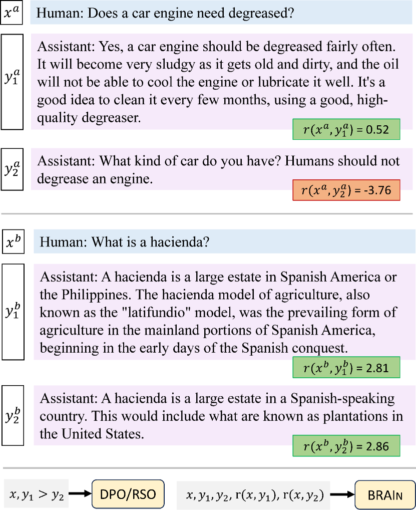
Figure 1: Two examples used for training alignment algorithms with different reward situations: one where the rewards have a big gap, and another where the gap is smaller.

Rewards obtained using an RM trained on human preference convey additional fine-grained information about the outputs. Consider the two cases in Figure 1. In the first example, one output is clearly better than the other. Whereas, in the second example, both outputs are almost equally good. Therefore the first example is more important for alignment than the second example. The gap in reward scores captures this importance. Recent alignment models such SLiC, RRHF, and DPO ignore this crucial fine-grained RM information.

In this work, we develop an alignment method that returns to a more explicit use of RMs but retains the scalability of recent techniques. For this, we propose BRAIn: Bayesian Reward-conditioned Amortized Inference. BRAIn starts from a different principle than PPO or DPO, which focuses on regularized reward maximization. Here we aim to distill the reward-conditioned posterior $p({y}|x,G=1)$, understood as conditioning the prior distribution $p(y\mid x)$ (SFT model) to obtain only outputs that are deemed good ($G=1$).

Instead of training a reward-conditioned model, such as Quark (Lu et al., 2022), that first takes both prompt $x$ and quantized reward as input while training and then freezes reward to a high value during inference, BRAIn directly distills the posterior distribution with fixed $G=1$ into an amortized policy parameterized by an LLM.

The connection with RMs is attained by decomposing the posterior via Bayes theorem and parametrizing the likelihood, a Goodness model $p(G=1|{y},x)$, with the reward function. To sample from the posterior, BRAIn leverages self-normalised importance sampling ratios (Owen, 2013). To reduce the variance of the gradient (Schulman et al., 2017; Ziegler et al., 2019; Sutton et al., 1999), we propose a novel self-normalized baseline and prove that the baseline-subtracted gradient estimate is an unbiased estimator of a divergence measure that we refer to as self-normalized KL divergence.

In our experiments on TL;DR summarization (Stiennon et al., 2020; Völske et al., 2017) and AntropicHH (Bai et al., 2022), BRAIn establishes a new state-of-the-art by significantly outperforming existing s-o-t-a RL method DPO (Rafailov et al., 2023). In addition, we bridge the gap between BRAIn and DPO by careful augmentation of DPO objective in two ways. Specifically, we incorporate: 1) multiple outputs for a given input prompt, and 2) reward as an importance weight in the DPO objective.

Overall, we make the following contributions:

1. We propose BRAIn, a novel algorithm to align an LLM to human-preferences. Unlike existing ranking-based methods, BRAIn incorporates fine-grained reward scores while training. BRAIn uses a novel self-normalized baseline for variance reduction of the proposed gradient estimate.

2. We theoretically prove that the proposed gradient estimate is an unbiased estimator of a modified form of KL divergence that we name BRAIn objective.

3. We derive the exact form of the BRAIn objective under Bradley-Terry preference model assumption. We also show DPO can be derived as a special case of the BRAIn objective.

4. Finally, we empirically substantiate our claims by experimenting on two natural language generation tasks.

2 Related Works

In relation to RLHF approaches, InstructGPT (Ouyang et al., 2022) made fundamental contributions to conversational agent alignment and showed how Proximal Policy Optimization (PPO) (Schulman et al., 2017) could be used for this purpose. PPO is however a type of online-RL algorithm which carries high costs of sampling and keeping additional LLMs in memory, such as value networks.

After PPO, offline-RL algorithms have emerged. SLiC (Zhao et al., 2023) proposed a margin loss between the likelihood (log probability) of the preferred output $y_{w}$ and the rejected output $y_{\ell}$ and adds the cross entropy over the SFT dataset as a soft regularizer in its training objective. RRHF (Yuan et al., 2023) extends this idea to multiple outputs $y_{i},1\leq i\leq n$, for the same input using a ranking loss. Both methods may use Rewards implicitly to obtain the output preference but can not incorporate reward values directly.

DPO has found clear success in aligning LLMs (Tunstall et al., 2023; Ivison et al., 2023), however augmenting the training data by sampling outputs from SFT model and using RM to rate them is infeasible.

RSO Liu et al. (2023) revisits SLiC and DPO but considers sampling from the optimal policy of the PPO objective. For comparision purposes, RSO can be considered as an improvement to DPO. Compared to these approaches, BRAIn shares the lower costs of the ranking-based methods while explicitly using the fine-grained rewards.

Related to learning distributions conditioned on desired features, earlier works such as Ficler & Goldberg (2017), train special feature embeddings to produce text with desired target features. More recently Chen et al. (2021) conditions on a goodness token, and (Lu et al., 2022; Korbak et al., 2023) threshold a reward model for the same purpose. Although inspired by reward conditioning, BRAIn deviates from these approaches by not explicitly parametrizing the conditional distribution that takes both prompt $x$ and desired reward as input. Instead, BRAIn poses the problem as distributional matching of the posterior distribution. The use of conditional training models for RLHF has also been limited (Korbak et al., 2023) since they are not considered very performant.

Related to distributional matching approaches leveraging importance sampling, Korbak et al. (2022) models the desired target distribution as an Energy-Based Model (EBM) (Teh et al., 2003) over the reward function and use Distributional Policy Gradients (Parshakova et al., 2019) to train the policy. This work also leverages importance sampling with variance reduction for this purpose. By comparison, our work does not assume any specific form for the desired target distribution. Instead, BRAIn treats the reward-conditioned posterior as its target and exploits the reward modelling assumptions (Bradley-Terry etc.) to compute the posterior distribution. Further, compared to these approaches, BRAIn introduces a novel self-normalized variance reduction method with a strong impact on performance and theoretical justification.

3 Notation

Let $x$ be an input prompt and $\mathcal{Y}$ be the set of all output sequences. Let $p({y}|x)$ be the conditional probability assigned by a supervised fine-tuned (SFT) language model (LM) to an output $y\in\mathcal{Y}$ for an input $x$. Let $r(x,{y})$ be the corresponding reward value assigned by a given reward function. Further, let $G$ represent a binary random variable such that the probability $p(G=1|{y},x)$ captures the goodness of a given output $y$ for a given input $x$. The relationship between probability $p(G=1|{y},x)$ and reward value $r(x,{y})$ depends upon the modelling assumptions made while training the reward model. In section 5.1, we illustrate the connection between $p(G=1|{y},x)$ and $r(x,{y})$ for both absolute and relative reward models such as Bradley-Terry.

Given the prior $p({y}|x)$, and the goodness model $p(G=1|{y},x)$, we define the posterior $p({y}|x,G=1)$ as our desired distribution that assigns high probability to ‘good’ outputs. To mimic sampling from the posterior distribution, we aim to train a new model $q_{\theta}({y}|x)$ by minimizing the KL divergence between the two.

4 Approach

Bayesian reformulation: We first use Bayes’ rule to represent the reward–conditioned posterior as:

$$p({y}|x,G=1)=\frac{p({y}|x)p(G=1|{y},x)}{p(G=1|x)}$$ (1)

We are interested in sampling from $p({y}|x,G=1)$, i.e., samples with high reward. An obvious solution is to sample from $p({y}|x)$ and keep rejecting the samples until a sample with a high reward is obtained. Despite its simplicity, rejection sampling is expensive. Hence, in this work, we propose to learn a distribution, $q_{\theta}({y}|x)$, that can mimic sampling from the posterior without the computation overhead of rejection sampling.

Training objective: To train the parameters $\theta$, we propose to minimize the KL–divergence between the posterior distribution $p({y}|x,G=1)$, and $q_{\theta}({y}|x)$. This is equivalent to maximizing the objective:

$$\mathcal{L}_{x}(\theta) =-\mathbb{E}_{p({y}|x,G=1)}\left[\log\frac{p({y}|x,G=1)}{q_{\theta}({y}|x)}\right]$$ (2)

By collecting all the constant terms with respect to $\theta$ in $C$, the objective can be written as

$$\mathcal{L}_{x}(\theta) =\mathbb{E}_{p({y}|x,G=1)}\left[\log q_{\theta}({y}|x)\right]+C\,$$ (3)

Henceforth, the constant $C$ will be omitted in subsequent formulations of the objective $\mathcal{L}_{x}(\theta)$.

Approximation with importance sampling: To empirically compute the expectation in eq. 4, we need to sample from the posterior $p({y}|x,G=1)$. Unfortunately, it is not possible to do so directly, and hence we resort to importance sampling (Tokdar & Kass, 2010),

$$\mathcal{L}_{x}(\theta) =\mathbb{E}_{q^{\prime}({y}|x)}\left[\frac{p({y_{i}}|x,G=1)}{q^{\prime}({y_{i}}|x)}\log q_{\theta}({y}|x)\right]\,$$ (4)

where $q^{\prime}({y}|x)$ is an an easy–to–sample proposal distribution. Taking into account the Bayes rule in equation (1) we approximate the expectation by a sample average of $n$ outputs $(y_{1},\ldots y_{n})$ from $q^{\prime}({y}|x)$. We further use self–normalized importance sampling (ch. 9 in Owen (2013)), normalizing the weights by their sum. This results in the following loss for a given $x$:

$$\hat{\mathcal{L}}_{x}(\theta)=\sum_{i=1}^{n}\hat{\alpha}_{y_{i}}\log q_{\theta}({y_{i}}|x)\text{, where }y_{i}\sim q^{\prime}({y}|x)$$ (5)

$$\hat{\alpha}_{y_{i}}=\frac{\alpha_{y_{i}}}{\sum_{j=1}^{n}\alpha_{y_{j}}}\text{ , }\alpha_{y_{i}}=\frac{p({y_{i}}|x)}{q^{\prime}({y_{i}}|x)}p(G=1|{y_{i}},x)$$ (6)

Note that we dropped $p(G=1|x)$ from $\alpha_{y_{i}}$ as it will get cancelled due to self–normalization. We have added subscripts to $\alpha$ to show that they depend on the samples $y$. The gradient of the objective can be written as

$$\nabla_{\theta}\hat{\mathcal{L}}_{x}(\theta)=\sum_{i=1}^{n}\hat{\alpha}_{y_{i}}\nabla_{\theta}\log q_{\theta}({y_{i}}|x)$$ (7)

Baseline subtraction: One critical issue with the loss in eq. 5 is that it assigns a positive weight to all the samples $y_{i}$ for a given $x$, irrespective of its reward distribution $p(G=1|{y_{i}},x)$. We empirically observed (see Section 9.3) that this results in very slow convergence for large output spaces common in natural language.

To introduce competition among the outputs (and thereby reduce the variance of the gradient estimate), a common technique in reinforcement learning literature (Greensmith et al., 2004; Korbak et al., 2022) is to subtract a suitable baseline from the gradient estimate of the RL objective. One must ensure that subtracting the baseline introduces minimal (if any) bias in the gradient estimate of the objective.

To obtain such a baseline for our case, we first note the following general result (derived for $q_{\theta}({y}|x)$ here),

$$\mathbb{E}_{q_{\theta}({y}|x)}\nabla_{\theta}\log q_{\theta}({y}|x)=\mathbb{E}_{q_{\theta}({y}|x)}\frac{1}{q_{\theta}({y}|x)}\nabla_{\theta}q_{\theta}({y}|x)$$ (8)

$$=\sum_{y\in\mathcal{Y}}\nabla_{\theta}q_{\theta}({y}|x)=\nabla_{\theta}\sum_{y\in\mathcal{Y}}q_{\theta}({y}|x)=\nabla_{\theta}1=0$$ (9)

Thus, this expectation can be subtracted from the gradient in (7) without introducing any bias. To estimate the baseline, we reuse the same samples $(y_{1},\ldots,y_{n})$ that are used in (5) and apply self–normalized importance sampling to get:

$$\mathbb{E}_{q_{\theta}({y}|x)}\nabla_{\theta}\log q_{\theta}({y}|x)\approx\sum_{i=1}^{n}\hat{\beta}_{y_{i}}\nabla_{\theta}\log q_{\theta}({y_{i}}|x)$$ (10)

$$y_{i}\sim q^{\prime}({y}|x)\text{ and }\hat{\beta}_{y_{i}}=\frac{\beta_{y_{i}}}{\sum_{j=1}^{n}\beta_{y_{j}}}\text{ , }\beta_{y_{i}}=\frac{q_{\theta}({y_{i}}|x)}{q^{\prime}({y_{i}}|x)}$$ (11)

Subtracting the baseline estimate from eq. 7, we get:

$$\nabla_{\theta}\hat{\mathcal{L}}_{x}(\theta)=\sum_{i=1}^{n}\left(\hat{\alpha}_{y_{i}}-\hat{\beta}_{y_{i}}\right)\nabla_{\theta}\log q_{\theta}({y_{i}}|x)$$ (12)

$y_{i},\hat{\alpha}_{y_{i}},\text{and }\hat{\beta}_{y_{i}}$ are same as in eqs. 6 and 11. We call the self-normalized baseline subtracted gradient estimate in (12) as the BRAIn gradient estimate. Intuitively, $\alpha_{y_{i}}$ and $\beta_{y_{i}}$ are proportional to the posterior $p({y_{i}}|x,G=1)$ and policy $q_{\theta}({y_{i}}|x)$ distributions, respectively. Thus, the weight (difference of normalized $\alpha_{y_{i}}$ and $\beta_{y_{i}}$) of each $y_{i}$ captures how far the current estimate of policy $q_{\theta}({y_{i}}|x)$ is from the true posterior $p({y_{i}}|x,G=1)$. This also alleviates the critical issue of assigning positive weights to all $y_{i}$ irrespective of their reward. Samples with lower reward, and hence lower posterior $p({y_{i}}|x,G=1)$ (consequently lower $\alpha_{y_{i}}$), will get negative weights as soon as the policy distribution $q_{\theta}({y_{i}}|x)$ assigns higher probability to them (consequently higher $\beta_{y_{i}}$) than the posterior, and vice-versa.

Algorithm 1 Bayesian Reward-conditioned Amortized Inference

0:  $r(x,y),p(y|x),D,e,m,n,k$

1:  Initialize $q^{\prime}(y|x)\leftarrow p(y|x)$, $q_{\theta}(y|x)\leftarrow p(y|x)$

2:  Initialize $D_{0}\leftarrow\{\}$

3:  for $t=1$ to $e$ do

4:     $S_{t}\leftarrow$ randomly selected $m$ prompts from $D$

5:     for all $x\in S_{t}$ do

6:        $Y_{x}\leftarrow$ generate $n$ samples using $q^{\prime}(y|x)$

7:        for all $y\in Y_{x}$ do

8:           Cache $\log q^{\prime}(y|x),\log p(y|x),r(x,y)$ in $S_{t}$

9:           Cache normalized $\hat{\alpha}_{y}$ (eq. 6 or eq. 20) in $S_{t}$

10:        end for

11:     end for

12:     $D_{t}\leftarrow D_{t-1}\cup S_{t}$

13:     for $j=1$ to $k$ do

14:        $B\leftarrow$ randomly sampled batch from $D_{t}$

15:        for all $(x,Y_{x},q^{\prime}(y|x),\hat{\alpha}_{y})\in B$ do

16:           Compute $\hat{\beta}_{y}$ (eq. 11)

17:           $\mathcal{L}_{x}(\theta)\leftarrow\sum_{y\in Y_{x}}(\hat{\alpha}_{y}-\hat{\beta}_{y})\log q_{\theta}({y}|x)$

18:        end for

19:        Update $\theta$ using $\nabla_{\theta}\sum_{x\in B}\mathcal{L}_{x}(\theta)$

20:     end for

21:     $q^{\prime}({y}|x)\leftarrow q_{\theta}({y}|x)$

22:  end for

23:  Return $q_{\theta}$

The BRAIn algorithm with the self-normalized baseline is given in Algorithm 1. We initialize both our proposal $q^{\prime}({y}|x)$ and policy $q_{\theta}({y}|x)$ with $p({y}|x)$. We update the proposal $e$ times after every $k$ gradient updates. $m$ is the number of prompts sampled from dataset $D$ after updating the proposal, and $n$ is the number of outputs generated for each prompt $x\in D$.

In our experiments, we show that subtracting the self–normalized baseline results in a tremendous improvement in performance. We hypothesize that the baseline allows the model to focus on distinctive features of high-reward outputs compared to the lower-reward ones.

A formal justification of the biased gradient estimate: Self-normalized importance sampling (SNIS) introduces bias in any estimator. In this paper, we have used SNIS to approximate the importance weights as well as the baseline in our gradient estimate. Using biased gradient estimators for training often results in optimization of an objective different from the desired one.

However, in our case, we show that using the BRAIn gradient estimate for training, results in minimizing a self-normalized version of KL–divergence (defined below) whose minimum value is achieved only when $q_{\theta}({y}|x)=p({y}|x,G=1)$. Note that this is a consequence of the chosen self-normalized baseline in (11).

First, we define self-normalized KL divergence in the context of this paper. Next, we show that our proposed BRAIn gradient estimate is an unbiased estimator of the gradient of this divergence measure. Finally, we prove that this self-normalized KL divergence is non-negative and equals $0$ only when the policy learns to mimic the posterior. The proofs are in appendix A.

Definition 4.1.

Let the proposal distribution $q^{\prime}({y}|x)$, training policy $q_{\theta}({y}|x)$ and posterior $p({y}|x,G=1)$ be as defined earlier. Furthermore, we assume that $\text{support}(p)\subseteq\text{support}(q_{\theta})\subseteq\text{support}(q^{\prime})$. For any $n$ outputs, $Y_{x}=({y}_{1},\ldots,{y}_{n})$, let $\hat{\alpha}_{y_{i}}$ and $\hat{\beta}_{y_{i}}$ be the self–normalized importance sampling weights for the loss and the baseline, respectively (eqs. 6 and 11). The self-normalized KL–divergence between the posterior and training policy for the given proposal distribution is defined as:

$$D_{n}^{q^{\prime}}(p({y}|x,G=1)||q_{\theta}({y}|x))$$

$$=\mathbb{E}_{\begin{subarray}{c}y_{i}\sim q^{\prime}({y}|x)\\ 1\leq i\leq n\end{subarray}}\left[D_{KL}(\hat{\alpha}_{Y_{x}}||\hat{\beta}_{Y_{x}})\right]\text{ where }$$ (13)

$$D_{KL}(\hat{\alpha}_{Y_{x}}||\hat{\beta}_{Y_{x}})=\sum_{i=1}^{n}\hat{\alpha}_{y_{i}}\log\frac{\hat{\alpha}_{y_{i}}}{\hat{\beta}_{y_{i}}}$$ (14)

Theorem 4.2.

The BRAIn gradient estimate defined in (12) is an unbiased estimator of the gradient (w.r.t. $\theta$) of negative self-normalized KL–divergence between the posterior $p({y}|x,G=1)$ and training policy $q_{\theta}({y}|x)$ defined in (13). Here, the dependence of KL divergence on $\theta$ comes from $\hat{\beta}_{y_{i}}$ being a function of $q_{\theta}({y_{i}}|x)$.

Since the gradient of our objective in eq. 12 is the same as the gradient of negative self-normalized KL-divergence defined in eq. 13, in the rest of the paper, we refer to negative self-normalized KL-divergence between the posterior and the training policy as BRAIn objective.

Theorem 4.3.

The self-normalized KL–divergence defined in (13) reaches its minimum value of $0$ if and only if the KL–divergence between the posterior and training policy also reaches $0$. Also, $q_{\theta}({y}|x)=p({y}|x,G=1)$ is the only minima of self-normalized KL–divergence defined in (13).

5 Goodness Model and the reward function

In this section, we demonstrate how the modelling assumptions of the reward function shape the relationship between the goodness model $p(G=1|{y},x)$ and the reward function $r(x,{y})$. A logistic regression reward model trains a binary classifier to distinguish human-preferred outputs, e.g., a positive sentiment classifier. In such scenarios, the goodness model $p(G=1|{y},x)$ can be defined as:

$$p(G=1|{y},x)=\sigma(r(x,{y}))$$ (15)

For Bradley-Terry models, we use the observation that due to self–normalization of $\alpha_{y_{i}}$’s in (12), we need not compute the value $p(G=1|{y_{i}},x)$ explicitly, but only the ratio $p(G=1|{y_{i}},x)/p(G=1|{y_{j}},x)$.

5.1 Bradley-Terry Preference Model for LLMs

Given an absolute goodness measure $g_{i}$ for each $y_{i}$, Bradley-Terry Model (BTM) defines the probability of choosing $y_{i}$ over $y_{j}$ as:

$$\mathbb{P}(y_{i}\succ y_{j})=\frac{g_{i}}{g_{i}+g_{j}}$$ (16)

Recall that in our formulation, the binary random variable $G$ represents the goodness of an output, and hence, the conditional probability $p(G=1|{y_{i}},x)$ can be used as a proxy for $g_{i}$:

$$\mathbb{P}(y_{i}\succ y_{j}|x)=\frac{p(G=1|{y_{i}},x)}{p(G=1|{y_{i}},x)+p(G=1|{y_{j}},x)}$$ (17)

During training of the reward function $r(x,{y})$, we are given triplets $(x,y_{i},y_{j})$ such that for an input $x$, the response $y_{i}$ is preferred over the response $y_{j}$. We train it by maximizing the log-likelihood over all the training triplets. During training, the goodness measure $g_{i}$ is parameterized as $\exp{(r(x,y_{i}))}$ resulting in the following log-likelihood of a triplet:

$$\log\mathbb{P}(y_{i}\succ y_{j}|x)=\log\sigma\left(r(x,{y_{i}})-r(x,{y_{j}})\right)$$ (18)

Thus, by equating eq. 18 and log of eq. 17, we get the maximum likelihood estimate of the log–odds as:

$$\log\frac{p(G=1|{y_{i}},x)}{p(G=1|{y_{j}},x)}=r(x,{y_{i}})-r(x,{y_{j}})$$ (19)

The above ratio is exactly what we need to compute self–normalized importance weights $\alpha_{y_{i}}/\sum_{j=1}^{n}\alpha_{y_{j}}$ in eq. 5. We formalize this result in the proposition below.

Proposition 5.1.

For the Bradley-Terry preference model defined in eq. 17 and parameterized by eq. 18, the self–normalized importance-weights $\hat{\alpha}_{y_{i}}=\alpha_{y_{i}}/\sum_{j=1}^{n}\alpha_{y_{j}}$ have the following form:

$$\frac{\exp(r(x,{y_{i}})+\log p({y_{i}}|x)-\log q^{\prime}({y_{i}}|x))}{\sum_{j=1}^{n}\exp(r(x,{y_{j}})+\log p({y_{j}}|x)-\log q^{\prime}({y_{j}}|x))}$$ (20)

In the special case where the proposal distribution $q^{\prime}({y}|x)$ is the same as the prior distribution $p({y}|x)$, the importance weights reduces to

$$\hat{\alpha}_{y_{i}}=\frac{\exp(r(x,{y_{i}}))}{\sum_{j=1}^{n}\exp(r(x,{y_{j}}))}$$ (21)

See the appendix for the proof. Observe that $\hat{\alpha}_{y_{i}}$ in eq. 21 is nothing but a softmax over the reward values $r(x,{y_{i}})$. In the next section, we show that DPO is a special case of our formulation when we replace softmax with argmax and set $n=2$. This amounts to assigning all the importance weight to the output sample with the most reward.

6 DPO as a special case of BRAIn

In DPO (Rafailov et al., 2023), an ideal setting is discussed where the samples are generated from the base policy ($p({y}|x)$ in our case) and annotated by humans. Often, the preference pairs in publicly available data are sampled from a different policy than $p({y}|x)$. To address this, Liu et al. (2023) experiment with a variant of DPO, called DPO-sft, in which a reward model is first trained on the publicly available preference pairs and then used for annotating the samples generated from the base policy $p({y}|x)$.

We claim that BRAIn reduces to DPO-sft when we generate only 2 samples per input $x$ and assign all the importance weight $\hat{\alpha}_{y_{i}}$ only to the winner. The last assumption is equivalent to replacing softmax in eq. 21 with an argmax. We formalize it in the theorem below:

Theorem 6.1.

Let the proposal distribution $q^{\prime}({y}|x)$ in BRAIn be restricted to the prior $p({y}|x)$. When $n=2$, and the softmax is replaced by argmax in eq. 21, then the BRAIn objective reduces to DPO objective proposed by Rafailov et al..

Proof.

We start with BRAIn objective defined in eq. 13 and insert our assumptions to arrive at DPO objective.

By subsituting $n=2$ and $q^{\prime}({y}|x)=p({y}|x)$ in R.H.S. of eq. 13, and using eq. 14, we get:

$$\mathbb{E}_{\begin{subarray}{c}y_{1},y_{2}\sim p({y}|x)\end{subarray}}\left[\hat{\alpha}_{y_{1}}\log\frac{\hat{\alpha}_{y_{1}}}{\hat{\beta}_{y_{1}}}+\hat{\alpha}_{y_{2}}\log\frac{\hat{\alpha}_{y_{2}}}{\hat{\beta}_{y_{2}}}\right]$$ (22)

Now, without loss of generality, assume that $r(x,{y_{1}})>r(x,{y_{2}})$. Replacing softmax with argmax in eq. 21, we get $\hat{\alpha}_{y_{1}}=1$ and $\hat{\alpha}_{y_{2}}=0$. Plug it in eq. 22 to get:

$$-\mathbb{E}_{\begin{subarray}{c}y_{1},y_{2}\sim p({y}|x)\end{subarray}}\log\hat{\beta}_{y_{1}}$$

Now recall from eq. 11 that $\hat{\beta}_{y_{1}}=\beta_{y_{1}}/(\beta_{y_{1}}+\beta_{y_{2}})$ and $\beta_{y_{i}}=\frac{q_{\theta}({y_{i}}|x)}{p({y_{i}}|x)}$. Replacing it in the above equation and rearranging the terms, we get:

$$-\mathbb{E}_{\begin{subarray}{c}y_{1},y_{2}\sim p({y}|x)\end{subarray}}\log\sigma\left(\log\frac{q_{\theta}({y_{1}}|x)}{p({y_{1}}|x)}-\log\frac{q_{\theta}({y_{2}}|x)}{p({y_{2}}|x)}\right)$$

The above expression is exactly same as equation (7) in Rafailov et al..

∎

We also note that to extend DPO to multiple outputs, i.e., $n>2$, Rafailov et al. resorts to a more general Plackett-Luce preference model. However, the datasets for training many of the publicly available reward models ((Stiennon et al., 2020; Bai et al., 2022)) do not follow Plackett-Luce assumptions for $n>2$.

7 Posterior and PPO-optimal policy

In this section, we show that for a Bradley-Terry reward model, the posterior $p({y}|x,G=1)$ corresponds to the PPO-optimal policy with the temperature parameter set to 1.

Theorem 7.1.

For a Bradley-Terry reward model, the posterior $p({y}|x,G=1)$ is same as the PPO optimal policy given by:

$$p^{*}({y}|x)=\frac{p({y}|x)\exp(r(x,{y}))}{\left(\sum_{\bar{y}\in\mathcal{Y}}p({\bar{y}}|x)\exp\left(r(x,{\bar{y}})\right)\right)}$$ (23)

The above eqn. for PPO optimal policy is as shown in equation(4) in Rafailov et al. (2023). Note that the reference policy in DPO is same as the prior policy in our formulation.

Proof.

We start with the definition of posterior in eq. 1, and use Bradley-Terry assumption to replace $p(G=1|{y},x)$ with a function of $r(x,{y})$.

In RHS of eq. 1, use total probability theorem to replace $p(G=1|x)$ with $\sum_{\bar{y}\in\mathcal{Y}}p({\bar{y}}|x)p(G=1|{\bar{y}},x)$ to get:

$$p({y}|x,G=1)=\frac{p({y}|x)p(G=1|{y},x)}{\sum_{\bar{y}\in\mathcal{Y}}p({\bar{y}}|x)p(G=1|{\bar{y}},x)}$$

Next, move $p({y}|x)p(G=1|{y},x)$ from the numerator to denominator:

$$p({y}|x,G=1)=\frac{p({y}|x)}{\left(\sum_{\bar{y}\in\mathcal{Y}}p({\bar{y}}|x)\frac{p(G=1|{\bar{y}},x)}{p(G=1|{y},x)}\right)}$$

Now, use eq. 19 to replace $\frac{p(G=1|{\bar{y}},x)}{p(G=1|{y},x)}$ in the denominator with $\exp\left(r(x,{\bar{y}})-r(x,{y})\right)$:

$$p({y}|x,G=1)=\frac{p({y}|x)}{\left(\sum_{\bar{y}\in\mathcal{Y}}p({\bar{y}}|x)\exp\left(r(x,{\bar{y}})-r(x,{y})\right)\right)}$$

Moving the common term $\exp(-r(x,{y}))$ from the denominator to numerator, we get:

$$p({y}|x,G=1)=\frac{p({y}|x)\exp(r(x,{y}))}{\left(\sum_{\bar{y}\in\mathcal{Y}}p({\bar{y}}|x)\exp\left(r(x,{\bar{y}})\right)\right)}$$

∎

8 Experimental Setup

Tasks: We conduct experiments on two natural language generation tasks, viz., summarization, and multi-turn dialog. In the summarization task, we align CarperAI’s summarization LM to a Bradley-Terry reward model. We train and evaluate using Reddit TL;DR dataset, in which input is a post on Reddit, and the aligned model should generate a high reward summary.
In the multi-turn dialog task, we ensure that a open-ended chatbot’s responses are Helpful and Harmless. We use QLoRA-tuned Llama-7b (Dettmers et al., 2023) as SFT model, and a fine-tuned GPT-J (Wang & Komatsuzaki, 2021) as the reward model. We train and evaluate using a subset of AntrophicHH (Bai et al., 2022) dataset. See section B.1 for hyperlinks to all the datasets and models described above.

Evaluation metrics: We use win–rate over gold responses and direct win–rate against the baseline responses to measure the performance of various techniques. Win–rate is defined as the fraction of test samples on which the generated response gets a higher reward than the gold response. We use two independent reward functions to compute the win–rate: (1) Train RM, which is the reward function used to align the SFT model, and (2) LLM eval, which follows LLM-as-a-judge (Zheng et al., 2023) and prompts a strong instruction following LLM, Mixtral-8x7B (Jiang et al., 2024), to compare the two outputs and declare a winner. The first metric captures the effectiveness of the alignment method in maximizing the specified reward, while a high win–rate using the LLM prompting ensures that the alignment method is not resorting to reward-hacking (Skalse et al., 2022).

Table 1: Win–rate (in %age) $\pm$ 95% confidence–interval against the gold output on the test sets. Train RM corresponds to the reward model used during training, whereas for LLM eval., we prompt Mixtral-8x7B.

AnthropicHH
	DPO	DPO-sft	RSO	BRAIn
Train RM	54.60$\pm$1.37	87.37$\pm$0.91	84.59$\pm$0.99	95.40$\pm$0.57
LLM eval	67.02$\pm$1.29	66.68$\pm$1.29	67.22$\pm$1.29	74.36$\pm$1.20
Reddit TL;DR
Train RM	86.72$\pm$0.82	90.86$\pm$0.70	91.24$\pm$0.68	95.21$\pm$0.52
LLM eval	60.26$\pm$1.18	60.55$\pm$1.18	60.41$\pm$1.18	64.74$\pm$1.16

We prompt GPT-4 (OpenAI et al., 2023) to directly compare BRAIn’s responses with each of the baselines separately. See section B.3 for the specific instructions used for prompting GPT-4 and Mixtral-8x7B.

Training details: While DPO uses human-annotated data directly, we generate $n=32$ samples per input prompt for the other models (DPO-sft, RSO, and BRAIn). The samples are organized in $16$ pairs for DPO-sft and RSO, while for BRAIn, the $32$ samples are grouped together. The model is evaluated after every $1,000$ steps and the best model is selected based on the win rate against the gold response on the cross-validation set. Other training details are given in Appendix B.2.

9 Experimental Results

Research Questions: Our experiments aim to assess BRAIn’s performance in aligning an SFT model to a given reward function and compare it against various baselines. Specifically, we answer the following research questions:

1. How does BRAIn compare to existing baselines?

2. How to bridge the gap between DPO and BRAIn?

3. What is the impact of baseline subtraction in BRAIn?

4. How does varying the number of output samples per input affect BRAIn’s performance?

5. Does periodically updating proposal distribution (step 21 in algorithm 1) help BRAIn?

9.1 Comparison with baselines

Table 1 compares the win–rate of BRAIn against our baselines – RSO, DPO, and DPO-sft. We observe that BRAIn consistently outperforms all the baselines, irrespective of the model used to compute win–rates. Specifically, when measured using the specified reward model, BRAIn achieves 8 and 4 pts better win–rate than the strongest baseline on AntrophicHH and TL;DR, respectively. Next, we observe that even though DPO-sft has a much better win–rate than DPO when computed using the specified reward function, their performance is the same when judged by an independent LLM, indicative of reward–hacking.

Table 2: Head-to-head comparison of the BRAIn against the baselines using GPT-4.

	AnthropicHH			Reddit TL;DR
	Win %	Tie %	Loss %	Win %	Tie %	Loss %
vs DPO	44.0	31.6	21.4	42.1	19.6	38.3
vs DPO-sft	45.4	34.4	20.2	45.2	18.9	35.9
vs RSO	44.2	35.5	20.3	45.1	17.6	37.3

In Table 2, we summarize the results of head-to-head comparisons of BRAIn with each of the baselines judged by GPT-4 on a set of 500 examples from each of the dataset. Win % indicates the percentage of examples for which BRAIn was declared the winner compared to the baseline. We observe that BRAIn wins twice as many times as the baselines on AnthropicHH.

9.2 Bridging the gap between DPO-sft and BRAIn

Table 3: Win–rates (in %age) obtained by incrementally augmenting DPO-sft; DPO-sft+IW: replace argmax by softmax; DPO-sft+IW+n: take softmax over $n=32$ outputs, instead of two outputs in 16 pairs

	DPO-sft	DPO-sft +IW	DPO-sft +IW+n	BRAIn
Train RM	87.37$\pm$0.91	89.21$\pm$0.85	93.30$\pm$0.69	95.40$\pm$0.57
LLM eval	66.78$\pm$1.29	69.28$\pm$1.27	73.89$\pm$1.21	74.36$\pm$1.17

In section 6, we show that under certain restrictions, BRAIn objective reduces to DPO-sft objective. In this section, we start with DPO-sft and relax these restrictions one at a time to demonstrate the impact of each restriction. First, we get rid of argmax and reintroduce softmax over rewards (eq. 21) to compute self–normalized importance weights $\hat{\alpha}_{y_{i}}$. This corresponds to the objective in eq. 22. We call this DPO-sft+IW. Next, we relax the assumption of $n=2$, and take softmax over $n=32$ outputs instead of softmax over two samples in 16 pairs. We call it DPO-sft+IW+n. Finally, we relax the restriction of proposal distribution to be the prior distribution only and instead update our proposal periodically (algorithm 1) to arrive at BRAIn.

Table 3 compares the win–rate of the two intermediate models (DPO-sft+IW, and DPO-sft+IW+n) with DPO-sft and BRAIn over the AntropicHH dataset. We first observe that relaxing each restriction consistently improves both the win–rates. The biggest gain ($\sim 4$ pts) comes by relaxing the assumption of $n=2$ and taking a softmax over all 32 outputs. This is expected as information contained in simultaneously comparing 32 outputs is potentially more than only 16 pairs. The gain by replacing argmax with softmax ($\sim 2$ pts) is similar to the gain by updating the proposal periodically, showing the importance of using the reward score.

9.3 Effect of baseline subtraction

In this experiment, we empirically assess the impact of our novel self-normalized baseline. To do so, we re-train the policies on the two datasets by setting $\hat{\beta}_{y}$ to $0$ for all $y\in Y_{x}$ in step (17) of algorithm 1. As expected, we observed a significant reduction in the performance. The win-rate using the specified reward model (Train RM) dropped from $95.21\%$ to $61.1\%$, and from $95.4\%$ to $58.3\%$ for TL;DR and AnthropicHH, respectively. This underscores the importance of baseline subtraction in gradient estimate of BRAIn.

9.4 Effect of the number of output samples

Next, we study the effect of varying the number of output samples ($n$) per input prompt $x$ on the performance of BRAIn. We retrain DPO-sft and BRAIn on AntropicHH dataset for each $n\in\{2,4,8,16,32\}$. As done earlier, we create $n/2$ pairs from the $n$ samples while training DPO-sft. The win–rates computed by specified reward model (Train RM) for each $n$ are plotted in fig. 2. We observe that including more samples in BRAIn objective leads to improvement in performance till $n=8$ after which it saturates, whereas the performance of DPO-sftimproves monotonically, albeit slowly.

Figure 2: Plot of Win-rate Against Gold as a function of the Number of Samples per Prompt.

9.5 Impact of periodically updating proposal distribution

In algorithm 1, we update the proposal distribution (step 21) after every $k$ gradient updates and add include new prompts with their samples from the latest policy. In this experiment, we re-train the policy without updating the proposal and instead always use the prior policy $p({y}|x)$ to generate samples for the new prompts. We observe $\sim 2$ pts reduction in win–rate using specified reward model on both the datasets. Specifically, it reduces from $95.4\%$ to $93.3\%$ on AnthropicHH dataset and from $95.21\%$ to $93.48\%$ on TL;DR summarization task.

10 Conclusion

In this paper, we propose an LLM alignment algorithm called BRAIn: Bayesian Reward-conditioned Amortized Inference. Like PPO, BRAIn uses fine-grained scores from the reward model, while maintaining the desirable scalability properties of more recent ranking techniques such as RSO and DPO. We propose a self-normalized variance reduction technique that significantly improves the performance. We show that under certain assumptions DPO is a special case of our proposed method. On standard TL;DR summarization and AnthropicHH datasets, BRAIn  performs better than existing state-of-the-art model alignment techniques such as DPO and RSO.

Appendix A Proof of Theorems

For the sake of completeness, we restate the definitions and the theorems here.

See 4.1 See 4.2

Proof.

For unbiasedness of the BRAIn gradient estimator, we need to show the following

$$\mathbb{E}_{\begin{subarray}{c}y_{i}\sim q^{\prime}({y}|x)\\ 1\leq i\leq n\end{subarray}}\sum_{i=1}^{n}\left(\hat{\alpha}_{y_{i}}-\hat{\beta}_{y_{i}}\right)\nabla_{\theta}\log q_{\theta}({y_{i}}|x)=-\nabla_{\theta}D_{n}^{q^{\prime}}(p({y}|x,G=1)||q_{\theta}({y}|x))\,,$$ (24)

where $\mathbf{y}=(y_{1},\ldots,y_{n})$ is a sequence of $n$ outputs, the values of $\alpha$ and $\beta$ are as defined in (6) and (11) respectively. The superscripts in $\alpha$ and $\beta$ denote their explicit dependence on the output sequence.

To prove the above, we expand each negative KL–divergence term in the self-normalized KL–divergence in terms of the entropy of normalized $\alpha_{y_{i}}$ and the cross-entropy between self-normalized $\alpha_{y_{i}}$ and $\beta_{y_{i}}$.

$$-D_{n}^{q^{\prime}}=\mathbb{E}_{\begin{subarray}{c}y_{i}\sim q^{\prime}({y}|x)\\ 1\leq i\leq n\end{subarray}}\left[\mathcal{H}\left(\hat{\alpha}_{y_{i}}\right)+\sum_{i=1}^{n}\hat{\alpha}_{y_{i}}\log\hat{\beta}_{y_{i}}\right]$$ (25)

Since the values $\alpha$ don’t depend on $\theta$, they are discarded during the gradient computation. Hence, the gradient can be written as

$$-\nabla_{\theta}D_{n}^{q^{\prime}}=\mathbb{E}_{\begin{subarray}{c}y_{i}\sim q^{\prime}({y}|x)\\ 1\leq i\leq n\end{subarray}}\sum_{i=1}^{n}\hat{\alpha}_{y_{i}}\nabla_{\theta}\left[\log\hat{\beta}_{y_{i}}\right]$$ (26)

Noting that $\hat{\beta}_{y_{i}}=\frac{\beta_{y_{i}}}{\sum_{j=1}^{n}\beta_{y_{j}}}$, we split the logarithm and compute the gradient of each term separately.

$$-\nabla_{\theta}D_{n}^{q^{\prime}} =\mathbb{E}_{\begin{subarray}{c}y_{i}\sim q^{\prime}({y}|x)\\ 1\leq i\leq n\end{subarray}}\sum_{i=1}^{n}\hat{\alpha}_{y_{i}}\left[\nabla_{\theta}\log\beta_{y_{i}}-\nabla_{\theta}\log\sum_{j=1}^{n}\beta_{y_{j}}\right]$$ (27)

$$=\mathbb{E}_{\begin{subarray}{c}y_{i}\sim q^{\prime}({y}|x)\\ 1\leq i\leq n\end{subarray}}\sum_{i=1}^{n}\hat{\alpha}_{y_{i}}\left[\nabla_{\theta}\log\beta_{y_{i}}-\frac{\sum_{j=1}^{n}\nabla_{\theta}\beta_{y_{j}}}{\sum_{j=1}^{n}\beta_{y_{j}}}\right]$$ (28)

Next, we note that $\nabla_{\theta}\beta_{y_{i}}=\beta_{y_{i}}\nabla_{\theta}\log\beta_{y_{i}}$ and

$$\nabla_{\theta}\log\beta_{y_{i}}=\nabla_{\theta}\left[\log q_{\theta}({y_{i}}|x)-\log q^{\prime}({y_{i}}|x)\right]=\beta_{y_{i}}\nabla_{\theta}\log q_{\theta}({y_{i}}|x)$$ (29)

Replacing these results back in equation (28), we get the desired result.

$$-\nabla_{\theta}D_{n}^{q^{\prime}} =\mathbb{E}_{\begin{subarray}{c}y_{i}\sim q^{\prime}({y}|x)\\ 1\leq i\leq n\end{subarray}}\sum_{i=1}^{n}\hat{\alpha}_{y_{i}}\left[\nabla_{\theta}\log q_{\theta}({y_{i}}|x)-\frac{\sum_{j=1}^{n}\beta_{y_{j}}\nabla_{\theta}\log q_{\theta}({y_{j}}|x)}{\sum_{j=1}^{n}\beta_{y_{j}}}\right]$$ (30)

$$=\mathbb{E}_{\begin{subarray}{c}y_{i}\sim q^{\prime}({y}|x)\\ 1\leq i\leq n\end{subarray}}\left[\frac{\sum_{i=1}^{n}\alpha_{y_{i}}\nabla_{\theta}\log q_{\theta}({y_{i}}|x)}{\sum_{j=1}^{n}\alpha_{y_{j}}}-\frac{\sum_{i=1}^{n}\beta_{y_{i}}\nabla_{\theta}\log q_{\theta}({y_{i}}|x)}{\sum_{j=1}^{n}\beta_{y_{j}}}\right]$$ (31)

$$=\mathbb{E}_{\begin{subarray}{c}y_{i}\sim q^{\prime}({y}|x)\\ 1\leq i\leq n\end{subarray}}\sum_{i=1}^{n}\left[\hat{\alpha}_{y_{i}}-\hat{\beta}_{y_{i}}\right]\nabla_{\theta}\log q_{\theta}({y_{i}}|x)$$ (32)

∎

See 4.3

Proof.

First, we will prove that $D_{KL}=0\implies D_{n}^{q^{\prime}}=0$ which is its minimum value. We note that the self-normalized KL–divergence is the weighted sum of KL–divergence between the normalized values of $\alpha$ and $\beta$. Hence, from the property of KL–divergence, it can’t be negative, that is, $D_{n}^{q^{\prime}}\geq 0$. Now, lets assume that $D_{KL}(p({y}|x,G=1)||q_{\theta}({y}|x))=0$. By the property of KL–divergence, this implies that $p({y}|x,G=1)=q_{\theta}({y}|x)\forall y\in\mathcal{Y}$. Thus:

$$\beta_{y_{i}}=\frac{q_{\theta}({y_{i}}|x)}{q^{\prime}({y_{i}}|x)}=\frac{p({y_{i}}|x,G=1)}{q^{\prime}({y_{i}}|x)}=\alpha_{y_{i}}$$ (33)

Incorporating it in the definition of self-normalized KL divergence in (13), we get:

$$D_{n}^{q^{\prime}} \left(p({y}|x,G=1)||q_{\theta}({y}|x)\right)=\mathbb{E}_{{\mathbf{y}}\sim q^{\prime}({y}|x)}\left[D_{KL}\left(\hat{\alpha}_{y_{i}}\left|\right|\hat{\alpha}_{y_{i}}\right)\right]=0$$ (34)

Instead of proving the other direction, we provide a constructive proof of its contrapositive, that is, $D_{KL}\neq 0\implies D_{n}^{q^{\prime}}\neq 0$. To see this, we note that $D_{KL}\neq 0$ implies the existence of at least one output, say $y_{+}$, where the posterior and policy disagree. Without loss of generality, lets assume that $p({y_{+}}|x,G=1)>q_{\theta}({y_{+}}|x)$. Since the probabilities must up to 1, there must exist at least one output, say $y_{-}$, for which $p({y_{-}}|x,G=1)<q_{\theta}({y_{-}}|x)$.

Since self-normalized KL-divergence $D_{n}^{q^{\prime}}$ has a KL-divergence $D_{KL}$ term for every sequence of length $n$, we construct a sequence $\mathbf{y}=(y_{+},y_{-},\ldots,y_{-})$. For such a sequence, all the values of $\alpha$ except the first one are equal. We note that the importance weight of the first output, that is $\alpha_{y_{+}}=\frac{p({y_{+}}|x,G=1)}{q^{\prime}({y_{+}}|x)}>\frac{q_{\theta}({y_{+}}|x)}{q^{\prime}({y_{+}}|x)}=\beta_{y_{+}}$. Similarly, the second importance weight $\alpha_{y_{-}}=\frac{p({y_{-}}|x,G=1)}{q^{\prime}({y_{-}}|x)}<\frac{q_{\theta}({y_{-}}|x)}{q^{\prime}({y_{-}}|x)}=\beta_{y_{-}}$. Combining these two results we get $\frac{\alpha_{y_{-}}}{\beta_{y_{-}}}<1<\frac{\alpha_{y_{+}}}{\beta_{y_{+}}}$. This can further be written as $\frac{\alpha_{y_{-}}}{\alpha_{y_{+}}}<\frac{\beta_{y_{-}}}{\beta_{y_{+}}}$.

Plugging in this result, the normalized values of $\alpha$ for the sequence are given by:

$$\frac{\alpha_{y_{1}}}{\sum_{j=1}^{n}\alpha_{y_{j}}}=\frac{\alpha_{y_{1}}}{\alpha_{y_{+}}+(n-1)\alpha_{y_{-}}}=\frac{1}{1+(n-1)\frac{\alpha_{y_{-}}}{\alpha_{y_{+}}}}>\frac{1}{1+(n-1)\frac{\beta_{y_{-}}}{\beta_{y_{+}}}}=\frac{\beta_{y_{+}}}{\beta_{y_{+}}+(n-1)\beta_{y_{-}}}=\frac{\beta_{y_{1}}}{\sum_{j=1}^{n}\beta_{y_{j}}}$$ (35)

Thus the KL–divergence term for this particular sequence, that is $D_{KL}\left(\hat{\alpha}_{y_{i}}||\hat{\beta}_{y_{i}}\right)$, is strictly greater than $0$. Since the support of proposal distribution includes the support of posterior and trainable policy, we get

$$D_{n}^{q^{\prime}}(p({y}|x,G=1)||q_{\theta}({y}|x))=\mathbb{E}_{{\mathbf{y}}\sim q^{\prime}({y}|x)}\left[D_{KL}\left(\hat{\alpha}_{y_{i}}||\hat{\beta}_{y_{i}}\right)\right]>0$$ (36)

Together with equation (34), this proves that $D_{KL}=0\implies D_{n}^{q^{\prime}}=0$ ∎

See 5.1

Proof.

The proof follows from the application of Bayes’ rule and the parameterization of Bradley-Terry model given in (19).

$$\hat{\alpha}_{y_{i}} =\frac{p({y_{i}}|x,G=1)/q^{\prime}({y_{i}}|x)}{\sum_{j=1}^{n}p({y_{j}}|x,G=1)/q^{\prime}({y_{j}}|x)}$$ (37)

$$=\frac{\frac{p({y_{i}}|x)}{q^{\prime}({y_{i}}|x)}\times\frac{p(G=1|{y_{i}},x)}{p(G=1|x)}}{\sum_{j=1}^{n}\frac{p({y_{j}}|x)}{q^{\prime}({y_{j}}|x)}\times\frac{p(G=1|{y_{j}},x)}{p(G=1|x)}}$$ (38)

$$=\frac{\frac{p({y_{i}}|x)}{q^{\prime}({y_{i}}|x)}\times p(G=1|{y_{i}},x)}{\sum_{j=1}^{n}\frac{p({y_{j}}|x)}{q^{\prime}({y_{j}}|x)}\times p(G=1|{y_{j}},x)}$$ (39)

$$=\frac{\frac{p({y_{i}}|x)}{q^{\prime}({y_{i}}|x)}}{\sum_{j=1}^{n}\frac{p({y_{j}}|x)}{q^{\prime}({y_{j}}|x)}\times\frac{p(G=1|{y_{j}},x)}{p(G=1|{y_{i}},x)}}$$ (40)

$$=\frac{\frac{p({y_{i}}|x)}{q^{\prime}({y_{i}}|x)}}{\sum_{j=1}^{n}\frac{p({y_{j}}|x)}{q^{\prime}({y_{j}}|x)}\times\exp{r(x,{y_{j}})-r(x,{y_{i}})}}$$ (41)

$$=\frac{\exp(r(x,{y_{i}})+\log p({y_{i}}|x)-\log q^{\prime}({y_{i}}|x))}{\sum_{j=1}^{n}\exp(r(x,{y_{j}})+\log p({y_{j}}|x)-\log q^{\prime}({y_{j}}|x))}$$ (42)

Here (38) follows by applying Bayes rule (see (1)) while (41) follows from the Bradley-Terry formulation in (19). If we set $q^{\prime}({y}|x)=p({y}|x)$, we get a softmax over the rewards as desired. ∎

Appendix B Details of Experimental Setup

B.1 Base models and datasets

In this section we provide links to all the publically available datasets and models used in our work.

We conduct experiments on two natural language generation tasks, viz., summarization, and multi-turn dialog. In the summarization task, we align CarperAI’s summarization LM to a Bradley-Terry reward model. We train and evaluate using Reddit TL;DR dataset, in which input is a post on Reddit, and the aligned model should generate a high reward summary.

In the multi-turn dialog task, we ensure that a open-ended chatbot’s responses are Helpful and Harmless. We use QLoRA-tuned Llama-7b (Dettmers et al., 2023) as SFT model, and a fine-tuned GPT-J (Wang & Komatsuzaki, 2021) as the reward model. We train and evaluate using a subset of AntrophicHH (Bai et al., 2022) dataset.

B.2 Other training details

All the models are trained using the PEFT and Transformers library. For Anthropic HH, we use QLoRA (Dettmers et al., 2023) for training BRAInand the other baselines. In particular, we use the same QLoRA hyperparameters (rank=$64$, $\alpha=16$) as used for supervised finetuning Llama-7B on Anthropic-HH dataset. We use the Adam optimizer(Kingma & Ba, 2014) with a learning rate of $1e-5$, weight decay of $0.1$ and $\beta_{1}$ and $\beta_{2}$ set to $0.9$ and $0.95$ respectively.

For summarization, we use LoRA(Hu et al., 2021) (rank=$8$, $\alpha=32$). The optimizer, learning rate, weight decay and and $\beta$ values are the same as for Anthropic HH.

B.3 Prompt for LLM-as-judge

In this section, we describe the prompts provided to the language models Mixtral-8x7B and GPT-4 for the purpose of comparing the gold standard outputs with the outputs generated by these models. The tasks involve acting as an impartial judge in evaluating responses or summaries provided by AI assistants.

B.3.1 Prompt for Anthropic HH

The prompt used for the Anthropic HH task is as follows:

”Please act as an impartial judge and evaluate the quality of the responses provided by the two AI assistants to the conversation displayed below. Your evaluation should consider correctness and helpfulness. You will be given a user conversation, assistant A’s answer, and assistant B’s answer. Your job is to evaluate which assistant’s answer is better based on the user conversation so far. Begin your evaluation by comparing both assistants’ answers with the user conversation so far. Identify and correct any mistakes. Avoid any position biases and ensure that the order in which the responses were presented does not influence your decision. Do not allow the length of the responses to influence your evaluation. Do not favor certain names of the assistants. Be as objective as possible. You should only evaluate the last utterance by both the assistants and not the full conversation. After providing your explanation, output your final verdict by strictly following this format: [̈[A]]ïf assistant A is better, [̈[B]]ïf assistant B is better, and [̈[C]]f̈or a tie.
————————————————–
{{Conversation}}
————————————————–
Assistant B
{{AssistantB}}
————————————————–
Assistant A
{{AssistantA}}
————————————————–”

B.3.2 Prompt for Summarization

The prompt used for the Summarization task is outlined below:

”Please act as an impartial judge and evaluate the quality of the tldrs or summaries provided by the two AI assistants to the reddit post displayed below. Begin your evaluation by comparing both assistants’ summaries with the reddit post so far. Do not allow the length of the summaries to influence your evaluation. After providing your explanation, output your final verdict by strictly following this format: [̈[A]]ïf assistant A is better, [̈[B]]ïf assistant B is better, and [̈[C]]f̈or a tie.
————————————————–
Reddit Post
{{Conversation}}
————————————————–
Assistant B
{{AssistantB}}
————————————————–
Assistant A
{{AssistantA}}
————————————————–”

References

- Bai et al. (2022) Bai, Y., Jones, A., and et al., K. N. Training a helpful and harmless assistant with reinforcement learning from human feedback, 2022.
- Chen et al. (2021) Chen, L., Lu, K., Rajeswaran, A., Lee, K., Grover, A., Laskin, M., Abbeel, P., Srinivas, A., and Mordatch, I. Decision transformer: Reinforcement learning via sequence modeling. Advances in neural information processing systems, 34:15084–15097, 2021.
- Dettmers et al. (2023) Dettmers, T., Pagnoni, A., Holtzman, A., and Zettlemoyer, L. Qlora: Efficient finetuning of quantized llms. arXiv preprint arXiv:2305.14314, 2023.
- Ficler & Goldberg (2017) Ficler, J. and Goldberg, Y. Controlling linguistic style aspects in neural language generation. In Brooke, J., Solorio, T., and Koppel, M. (eds.), Proceedings of the Workshop on Stylistic Variation, pp. 94–104, Copenhagen, Denmark, September 2017. Association for Computational Linguistics. doi: 10.18653/v1/W17-4912. URL https://aclanthology.org/W17-4912.
- Greensmith et al. (2004) Greensmith, E., Bartlett, P. L., and Baxter, J. Variance reduction techniques for gradient estimates in reinforcement learning. Journal of Machine Learning Research, 5(9), 2004.
- Hu et al. (2021) Hu, E. J., Shen, Y., Wallis, P., Allen-Zhu, Z., Li, Y., Wang, S., Wang, L., and Chen, W. Lora: Low-rank adaptation of large language models. arXiv preprint arXiv:2106.09685, 2021.
- Ivison et al. (2023) Ivison, H., Wang, Y., Pyatkin, V., Lambert, N., Peters, M., Dasigi, P., Jang, J., Wadden, D., Smith, N. A., Beltagy, I., et al. Camels in a changing climate: Enhancing lm adaptation with tulu 2. arXiv preprint arXiv:2311.10702, 2023.
- Jiang et al. (2024) Jiang, A. Q., Sablayrolles, A., Roux, A., Mensch, A., Savary, B., Bamford, C., Chaplot, D. S., de Las Casas, D., Hanna, E. B., Bressand, F., Lengyel, G., Bour, G., Lample, G., Lavaud, L. R., Saulnier, L., Lachaux, M., Stock, P., Subramanian, S., Yang, S., Antoniak, S., Scao, T. L., Gervet, T., Lavril, T., Wang, T., Lacroix, T., and Sayed, W. E. Mixtral of experts. CoRR, abs/2401.04088, 2024. doi: 10.48550/ARXIV.2401.04088. URL https://doi.org/10.48550/arXiv.2401.04088.
- Kingma & Ba (2014) Kingma, D. P. and Ba, J. Adam: A method for stochastic optimization. arXiv preprint arXiv:1412.6980, 2014.
- Korbak et al. (2022) Korbak, T., Elsahar, H., Kruszewski, G., and Dymetman, M. On reinforcement learning and distribution matching for fine-tuning language models with no catastrophic forgetting. Advances in Neural Information Processing Systems, 35:16203–16220, 2022.
- Korbak et al. (2023) Korbak, T., Shi, K., Chen, A., Bhalerao, R. V., Buckley, C., Phang, J., Bowman, S. R., and Perez, E. Pretraining language models with human preferences. In International Conference on Machine Learning, pp. 17506–17533. PMLR, 2023.
- Liu et al. (2023) Liu, T., Zhao, Y., Joshi, R., Khalman, M., Saleh, M., Liu, P. J., and Liu, J. Statistical rejection sampling improves preference optimization. arXiv preprint arXiv:2309.06657, 2023.
- Lu et al. (2022) Lu, X., Welleck, S., Hessel, J., Jiang, L., Qin, L., West, P., Ammanabrolu, P., and Choi, Y. Quark: Controllable text generation with reinforced unlearning. Advances in neural information processing systems, 35:27591–27609, 2022.
- OpenAI et al. (2023) OpenAI, :, Achiam, J., Adler, S., Agarwal, S., Ahmad, L., Akkaya, I., Aleman, F. L., Almeida, D., Altenschmidt, J., Altman, S., et al. GPT-4 technical report, 2023.
- Ouyang et al. (2022) Ouyang, L., Wu, J., Jiang, X., Almeida, D., Wainwright, C., Mishkin, P., Zhang, C., Agarwal, S., Slama, K., Ray, A., et al. Training language models to follow instructions with human feedback. Advances in Neural Information Processing Systems, 35:27730–27744, 2022.
- Owen (2013) Owen, A. B. Monte Carlo theory, methods and examples. https://artowen.su.domains/mc/, 2013.
- Parshakova et al. (2019) Parshakova, T., Andreoli, J., and Dymetman, M. Distributional reinforcement learning for energy-based sequential models. CoRR, abs/1912.08517, 2019. URL http://arxiv.org/abs/1912.08517.
- Rafailov et al. (2023) Rafailov, R., Sharma, A., Mitchell, E., Ermon, S., Manning, C. D., and Finn, C. Direct preference optimization: Your language model is secretly a reward model. arXiv preprint arXiv:2305.18290, 2023.
- Schulman et al. (2017) Schulman, J., Wolski, F., Dhariwal, P., Radford, A., and Klimov, O. Proximal policy optimization algorithms. arXiv preprint arXiv:1707.06347, 2017.
- Skalse et al. (2022) Skalse, J., Howe, N. H. R., Krasheninnikov, D., and Krueger, D. Defining and characterizing reward hacking. CoRR, abs/2209.13085, 2022. doi: 10.48550/ARXIV.2209.13085. URL https://doi.org/10.48550/arXiv.2209.13085.
- Stiennon et al. (2020) Stiennon, N., Ouyang, L., Wu, J., Ziegler, D. M., Lowe, R., Voss, C., Radford, A., Amodei, D., and Christiano, P. F. Learning to summarize from human feedback. CoRR, abs/2009.01325, 2020. URL https://arxiv.org/abs/2009.01325.
- Sutton et al. (1999) Sutton, R. S., McAllester, D., Singh, S., and Mansour, Y. Policy gradient methods for reinforcement learning with function approximation. Advances in neural information processing systems, 12, 1999.
- Teh et al. (2003) Teh, Y. W., Welling, M., Osindero, S., and Hinton, G. E. Energy-based models for sparse overcomplete representations. J. Mach. Learn. Res., 4:1235–1260, 2003. URL http://jmlr.org/papers/v4/teh03a.html.
- Tokdar & Kass (2010) Tokdar, S. T. and Kass, R. E. Importance sampling: a review. Wiley Interdisciplinary Reviews: Computational Statistics, 2(1):54–60, 2010.
- Touvron et al. (2023) Touvron, H., Martin, L., Stone, K., Albert, P., Almahairi, A., Babaei, Y., Bashlykov, N., Batra, S., Bhargava, P., Bhosale, S., et al. Llama 2: Open foundation and fine-tuned chat models. arXiv preprint arXiv:2307.09288, 2023.
- Tunstall et al. (2023) Tunstall, L., Beeching, E., Lambert, N., Rajani, N., Rasul, K., Belkada, Y., Huang, S., von Werra, L., Fourrier, C., Habib, N., et al. Zephyr: Direct distillation of lm alignment. arXiv preprint arXiv:2310.16944, 2023.
- Völske et al. (2017) Völske, M., Potthast, M., Syed, S., and Stein, B. Tl;dr: Mining reddit to learn automatic summarization. In Wang, L., Cheung, J. C. K., Carenini, G., and Liu, F. (eds.), Proceedings of the Workshop on New Frontiers in Summarization, NFiS@EMNLP 2017, Copenhagen, Denmark, September 7, 2017, pp. 59–63. Association for Computational Linguistics, 2017. doi: 10.18653/V1/W17-4508. URL https://doi.org/10.18653/v1/w17-4508.
- Wang & Komatsuzaki (2021) Wang, B. and Komatsuzaki, A. GPT-J-6B: A 6 Billion Parameter Autoregressive Language Model. https://github.com/kingoflolz/mesh-transformer-jax, May 2021.
- Ye et al. (2023) Ye, J., Chen, X., Xu, N., Zu, C., Shao, Z., Liu, S., Cui, Y., Zhou, Z., Gong, C., Shen, Y., Zhou, J., Chen, S., Gui, T., Zhang, Q., and Huang, X. A comprehensive capability analysis of gpt-3 and gpt-3.5 series models, 2023.
- Yuan et al. (2023) Yuan, Z., Yuan, H., Tan, C., Wang, W., Huang, S., and Huang, F. RRHF: Rank responses to align language models with human feedback without tears. arXiv preprint arXiv:2304.05302, 2023.
- Zhao et al. (2023) Zhao, Y., Joshi, R., Liu, T., Khalman, M., Saleh, M., and Liu, P. J. SLiC-HF: Sequence likelihood calibration with human feedback. arXiv preprint arXiv:2305.10425, 2023.
- Zheng et al. (2023) Zheng, L., Chiang, W., Sheng, Y., Zhuang, S., Wu, Z., Zhuang, Y., Lin, Z., Li, Z., Li, D., Xing, E. P., Zhang, H., Gonzalez, J. E., and Stoica, I. Judging llm-as-a-judge with mt-bench and chatbot arena. CoRR, abs/2306.05685, 2023. doi: 10.48550/ARXIV.2306.05685. URL https://doi.org/10.48550/arXiv.2306.05685.
- Ziegler et al. (2019) Ziegler, D. M., Stiennon, N., Wu, J., Brown, T. B., Radford, A., Amodei, D., Christiano, P., and Irving, G. Fine-tuning language models from human preferences. arXiv preprint arXiv:1909.08593, 2019.