EuLagNet: Eulerian Fluid Prediction with Lagrangian Dynamics

Abstract

Accurately predicting the future fluid is important to extensive areas, such as meteorology, oceanology and aerodynamics. However, since the fluid is usually observed from an Eulerian perspective, its active and intricate dynamics are seriously obscured and confounded in static grids, bringing horny challenges to the prediction. This paper introduces a new Lagrangian-guided paradigm to tackle the tanglesome fluid dynamics. Instead of solely predicting the future based on Eulerian observations, we propose the Eulerian-Lagrangian Dual Recurrent Network (EuLagNet), which captures multiscale fluid dynamics by tracking movements of adaptively sampled key particles on multiple scales and integrating dynamics information over time. Concretely, a EuLag Block is presented to communicate the learned Eulerian and Lagrangian features at each moment and scale, where the motion of tracked particles is inferred from Eulerian observations and their accumulated dynamics information is incorporated into Eulerian fields to guide future prediction. Tracking key particles not only provides a clear and interpretable clue for fluid dynamics but also makes our model free from modeling complex correlations among massive grids for better efficiency. Experimentally, EuLagNet excels in three challenging fluid prediction tasks, covering both 2D and 3D, simulated and real-world fluids.

1 Introduction

Figure 1: Comparison between Lagrangian and Eulerian perspectives. The left part presents the trajectory of five representative particles learned by EuLagNet in the Ocean Current dataset, which provides a Lagrangian perspective for the right Eulerian-recorded fluid.

Fluids, characterized by a molecular structure devoid of resistance to external shear forces, readily undergo deformation even under minimal force, thereby typically presenting extremely complex dynamics (Ferziger et al., 2020). Although theorems for fluid mechanics, such as Naiver-Stokes equations, have been widely explored for over a century, their solvability is confined to a limited subset of flows due to the complex form and intricate multiphysics interactions (Temam, 2001). In practical applications, computational fluid dynamics (CFD) is widely used to infer future fluid by numerical simulations but it suffers from huge computation costs due to the curse of dimensionality (Trunk, 1979). Till now, accurately predicting future dynamics is still a challenging problem. Recently, benefiting from the great non-linear modeling capability, deep models (Dissanayake & Phan-Thien, 1994; Raissi et al., 2017; Lu et al., 2021) have emerged as a promising tool for fluid prediction, which can be trained with CFD simulations or real-world observations and perform as a fast surrogate model during inference.

A booming direction for deep fluid prediction is learning deep models to solve governing partial differential equations (PDEs), such as Naiver-Stokes equations (Wang et al., 2023). One typical branch of these methods formalizes the PDE constraints along with initial and boundary conditions as the loss function of deep models (Weinan & Yu, 2017; Raissi et al., 2019; Wang et al., 2020a, b). However, they usually require exact formalizations for constraints and conditions, limiting their generality and applicability to real-world fluids that are usually partially observed. Another branch of methods proposes to utilize deep models to directly learn the neural operators between input and target functions, such as mappings between past observations and future predictions for fluid (Lu et al., 2021; Li et al., 2021, 2022; Wu et al., 2023; Li et al., 2023). Note that most of these methods attempt to capture fluid dynamics from the Eulerian perspective, which means the observation grid remains unchanged over time. However, capturing dynamics in the Eulerian space means modeling the spatiotemporal correlations among massive grids, which faces challenges in both computational efficiency and learning difficulties. Moreover, the active and intricate dynamics of fluids could be seriously obscured and confounded in static grids, making it hard to accurately predict future fluids.

Apart from the Eulerian method, we notice another approach for elucidating fluid dynamics (Gupta, 1988), that is the Lagrangian method, also known as the tracking method. This method primarily focuses on tracing individual fluid particles, that is conducting the temporal evolution process for the position and velocity of each particle. Unlike the Eulerian methods, the Lagrangian approach describes the fluid dynamics with the moving trajectory of individual fluid particles, offering a more natural and neat representation of fluid dynamics with inherent advantages in capturing intricate flow dynamics. As shown in Figure 1, we can find that fluid dynamics is much clearer in the Lagrangian trajectory than the density change on static Eulerian grids.

Inspired by the two perspectives mentioned above for describing fluid dynamics, we proposed Eulerian-Lagrangian Dual Recurrent Network, short as EuLagNet, aiming to integrate Lagrangian tracking into the deep model to assist the dynamics modeling in Eulerian fluid prediction. Concretely, a EuLag block is presented to accomplish Lagrangian tracking and Eulerian predicting at various scales. By leveraging the cross-attention mechanism, the EuLag block assimilates tracked particle dynamics into Eulerian space to guide fluid prediction. Simultaneously, we incorporate the principles of finite difference methods (Mitchell & Griffiths, 1980) into particle tracking and forecast the trajectory of tracked particles by learnable convolution kernels on the Eulerian space. The above-described Eulerian-Lagrangian dual design can take advantage of the dynamics information captured by Lagrangian trajectories and the fluid-structure feature learned in the Eulerian grid. Experimentally, EuLagNet achieves consistent state-of-the-art performance across three representative datasets, covering 2D and 3D fluid at various scales. Our contributions can be summarized as follows:

• Going beyond learning fluid dynamics at static grid points, we propose EuLagNet featuring the Eulerian-Lagrangian Dual Recurrent Network, which introduces the Lagrangian dynamics to assist fluid prediction by tracking essential fluid particles over time.

• Inspired by Lagrangian mechanics and finite difference methods, we present EuLag Block, which can accurately track particle movements and efficiently utilize the dynamic information of fluids in Eulerian prediction, enabling a better dynamic modeling paradigm.

• EuLagNet achieves consistent state-of-the art on three representative fluid prediction datasets with superior trade-offs for performance and efficiency, exhibiting favorable practicability for fluid across various scales.

2 Preliminaries

2.1 Eulerian and Lagrangian Descriptions

Eulerian and Lagrangian descriptions are two essential and foundational perspectives for describing fluid motion.

The Eulerian perspective is widely used in practical applications due to its convenience in data recording and analysis. In an Eulerian view, the fluid is observed at fixed points with accompanying physical quantities recorded. The Eulerian dynamics can be described as a function from fixed position $\mathbf{s}$ and time $\mathit{t}$ to velocity $\bm{v}=\bm{v}(\mathbf{s},\mathit{t})$. By integrating the velocity $\bm{v}$ along the temporal dimension and interpolating the results to observed grid points, we can obtain the future fluid in the subsequent steps (Ferziger et al., 2020).

Different from the static Eulerian view, the Lagrangian description focuses more on the trajectory of individual particles. Specifically, given one tracked fluid particle with initial position $\mathbf{s}_{0}$, the position function $\bm{d}=\bm{d}(\mathbf{s}_{0},\mathit{t})$ represents the relative displacement w.r.t. the initial position, which derives a trajectory of this particle. The intricate evolution of fluids in space can be revealed by tracking the motion of a set of particles (White, 2011). Thus, using the Lagrangian perspective makes it more convenient to describe complex phenomena, such as vortices and turbulence, by intuitively displaying the trajectory of each particle (Toro, 2009).

Since velocity is equal to the derivative of displacement w.r.t. time, these two perspectives of describing fluid are equivalent according to the following equation:

$$\bm{v}\left(\bm{d}(\mathbf{s}_{0},t),t\right)={\frac{\partial\bm{d}}{\partial t}}\left(\mathbf{s}_{0},t\right).$$ (1)

This equivalence inspires us to utilize Lagrangian descriptions for dynamics learning, which can free the model from complex spatiotemporal modeling in the Eulerian space.

2.2 Neural Fluid Prediction

Classical fluid prediction is based on computational fluid dynamics (CFD), which attempts to solve the governing dynamics equations through numerical methods. Yet, these methods usually take a few hours or even days for precise simulation (Umetani & Bickel, 2018). Deep learning methods have recently attracted great interest in fluid prediction, which can learn from data and provide a fast surrogate prediction during inference. One basic idea of these methods is to approximate the solution of governing equations of fluid based on the non-linear modeling capacity of deep models. The following two mainstreaming paradigms are presented.

Physics-informed neural networks (Raissi et al., 2017) are proposed for solving fluid equations, which formalize the governing equations as a loss function, and adopt deep models to learn the mapping from the coefficients of partial differential equations (PDEs) to its solution. This paradigm can precisely approximate the solution of PDEs. However, it typically requires the exact formalization of PDEs, such as the exact coefficient and boundary conditions for Navier-Stokes equations, thus difficult to apply to the partially observed real-world applications (Sim et al., 2021).

Figure 2: Overview of EuLagNet with multiscale Eulerian and Lagrangian features. At each time and scale, EuLag block accumulates the previous dynamics information to guide Eulerian feature evolution and predicts the particle movement conditioned on evolved features.

Recently, another paradigm has been widely explored in fluid prediction, that is learning neural operators to approximate the past-future mappings. First, Lu et al. (2021) proposed the DeepONet based on the universal approximation theorem. Afterward, FNO (Li et al., 2021) proposes to learn mapping in the frequency domain to approximate the temporal integral for fluid prediction. Subsequent FNO-based methods, such as Geo-FNO (Li et al., 2022), have improved upon it to accommodate irregular grids. Benefiting from the powerful long-sequence modeling capabilities of attention mechanisms, Galerkin Transformer (Cao, 2021) uses enhanced Galerkin attention to compute correlations between features with linear complexity. GNOT (Hao et al., 2023) uses ensemble information from the grid, equation parameters, and observations to learn efficient Transformers. FactFormer (Li et al., 2023) accelerates the computation process by applying a low-rank decomposition to the attention mechanism. Further, Wu et al. (2023) drew inspiration from spectral methods (Fornberg, 1998), solving PDEs through a linear combination of basis functions in a compact latent space obtained from attention. Although these methods can provide a relatively accurate solution to Navier-Stokes equations, all of them still capture the spatiotemporal correlations of fluid in the Eulerian space, where the intricate dynamics could be deeply confounded by the static grids, limiting their performance in complex scenarios, such as a fluid with complex boundaries. In contrast, EuLagNet tracks key particle movements from the Lagrangian perspective for fluids, thereby facilitating dynamics learning.

3 EuLagNet

To address the complex spatiotemporal correlations in Eulerian space, we present EuLagNet as a Eulerian-Lagrangian Dual Recurrent Network, which enables the collaborative learning of Eulerian features and Lagrangian dynamics at various scales by a newly designed EuLag block. Going beyond prior methods, projecting the dynamics learning from static Eulerian space to Lagrangian space will decompose the intricate spatiotemporal correlations into key trajectories, which can also benefit the computation efficiency.

Problem setup

Following the convention in operator learning (Li et al., 2021), we formalize the fluid prediction problem as learning operators between past observation functions to future fluid. Given a bounded open subset of $d$-dimension Eulerian space $\mathcal{D}\subset\mathbb{R}^{d}$, a fluid with $o$ observed quantities can be seen as functions of coordinates in Banach space $\mathcal{X}=\mathcal{X}(\mathcal{D};\mathbb{R}^{o})$. For each coordinate $\mathbf{s}\in\mathcal{D}$, $\bm{x}_{t}(\mathbf{s})\in\mathbb{R}^{o}$ and $\bm{x}_{t+1}(\mathbf{s})\in\mathbb{R}^{o}$ represent the fluid function between two consecutive time steps. Suppose that there are $P$ step observations, the fluid prediction process can be written as the following autoregressive paradigm:

$$\begin{split}\{\tilde{\bm{x}}_{t-P+1},\ldots,\tilde{\bm{x}}_{t}\}&\xrightarrow[]{\mathcal{F}_{\theta}}\tilde{\bm{x}}_{t+1}\\ \end{split}$$ (2)

where $t\geq P$ and $\mathcal{F}_{\theta}$ represents the neural operator with learnable parameters $\theta$. Here $\tilde{\bm{x}}_{t^{\prime}}=\bm{x}_{t^{\prime}}$ if $t^{\prime}\leq P$.

3.1 Eulerian-Lagrangian Dual Recurrent Network

It is widely recognized that fluid exhibits distinct motion characteristics at different scales (Cao, 2021; Wu et al., 2023). Thus, we design Eulerian-Lagrangian Dual Recurrent Network in a multiscale architecture to capture the fluid dynamics. Suppose that there are $L$ scales, as shown in Figure 2, we can obtain $t$-th step Eulerian representations at the $l$-th scale $\tilde{\bm{x}}_{t}^{l}:\mathcal{D}_{l}\to\mathbb{R}^{C_{l}}$ with downsampling $\operatorname{Down}()$:

$$\begin{split}\tilde{\bm{x}}_{t}^{l}=\operatorname{Down}(\tilde{\bm{x}}_{t}^{l-1}),\ \text{$l$ from $2$ to $L$},\\ \end{split}$$ (3)

where $\mathcal{D}_{l}\subset\mathbb{R}^{d}$ denotes the downsampled observation domain. $\tilde{\bm{x}}_{t}^{1}$ is encoded from past steps $\{\tilde{\bm{x}}_{t-P+1},\ldots,\tilde{\bm{x}}_{t}\}$ with $\mathcal{D}_{1}=\mathcal{D}$ through a learnable embedding layer.

At each scale, we adopt the EuLag block to incorporate the Lagrangian dynamics to guide Eulerian feature evolution. The process of $l$-th scale can be written as follows:

$$\begin{split}\tilde{\bm{x}}_{t+1}^{l},\{\mathbf{p}_{t+1}^{l,i}\},\{\mathbf{h}_{t}^{l,i}\}=\operatorname{EuLag}(\tilde{\bm{x}}_{t}^{l},\{\mathbf{p}_{t}^{l,i}\},\{\mathbf{h}_{t-1}^{l,i}\}),\\ \end{split}$$ (4)

where the set index is omitted. $\{\mathbf{p}_{t}^{l,i}\}_{i=1}^{M_{l}}$ represents the set of positions for $M_{l}$ tracked key particles with $\mathbf{p}_{t}^{l,i}\in\mathcal{D}_{l}$. $\{\mathbf{h}_{t}^{l,i}\}_{i=1}^{M_{l}}$ denotes the learned dynamics information with $\mathbf{h}_{t}^{l,i}\in\mathbb{R}^{C_{l}}$. EuLag block can take advantage of Lagrangian dynamics and Eulerian features simultaneously. More details about $\operatorname{EuLag}()$ are deferred in the next section.

Afterward, the evolved Eulerian features $\tilde{\bm{x}}_{t+1}^{l}$ are aggregated from bottom to top in sequence by upsampling $\operatorname{Up}()$:

$$\begin{split}\tilde{\bm{x}}_{t+1}^{l}=\operatorname{Up}(\tilde{\bm{x}}_{t+1}^{l},\tilde{\bm{x}}_{t+1}^{l+1}),\ \text{$l$ from $L-1$ to $1$}.\\ \end{split}$$ (5)

Eventually, the prediction $\tilde{\bm{x}}_{t+1}$ at step $t+1$ is decoded from $\tilde{\bm{x}}_{t+1}^{1}$ with a projection layer. More details of $\operatorname{Down}()$ and $\operatorname{Up}()$ are included in Appendix B.2.

3.2 EuLag Block

As formalized in Eq. (4), we adopt a dual recurrent framework to cooperatively utilize the Lagrangian dynamics and Eulerian representations, which consist of three successive steps: sampling Lagrangian particles, Lagrangian-guided feature evolving and Eulerian-conditioned particle tracking. For clarity, we omit the scale index in this section. The following features are all in the $l$-th scale.

Learning to sample Lagrangian particles

To attain the Lagrangian dynamics, we need to first choose several particles from the observation domain $\mathcal{D}$ as the viewpoints. Here we choose Lagrangian tracking particles via sampling from a data-adaptive learned distribution, which can make the model automatically focus on the essential zone of the fluid field. Technically, at the first predicting step, i.e. $t=P$, given deep Eulerian features observed on $N$ grids with $C$ channels $\tilde{\mathbf{x}}_{t}=\{\tilde{\bm{x}}_{t}(\textbf{s}_{k})|\textbf{s}_{k}\in\mathcal{D},1\leq k\leq N\}\in\mathbb{R}^{N\times C}$. The probability matrix of sampling $\mathbf{S}\in\mathbb{R}^{N}$ is obtained by:

$$\begin{split}\displaystyle\mathbf{S}=\operatorname{Softmax}\left(\operatorname{Conv}(\tilde{\mathbf{x}}_{t})\right).\end{split}$$ (6)

Here $\operatorname{Conv}()$ projects the $C$ channels into a single weight, which is subsequently normalized by $\operatorname{Softmax}()$ along the spatial dimension. Accordingly, $M$ tracking particles are sampled based on the probability matrix $\mathbf{S}$:

$$\begin{split}\displaystyle{\mathbf{p}_{t}}=\operatorname{Sample}(\{\mathbf{s}_{k}\}_{k=1}^{M},\mathbf{S}),\end{split}$$ (7)

where ${\mathbf{p}_{t}}=\{\mathbf{p}_{t,i}\}_{i=1}^{M}$ with $\mathbf{p}_{t,i}\in\mathcal{D}$. ${\mathbf{p}_{t}}$ represents the set of sampled $M$ particles, where $M$ is a hyperparameter.

Lagrangian-guided feature evolving

To extract essential dynamics information from the Eulerian field effectively, we first accumulate the dynamics along the tracking trajectory. Concretely, given previous dynamics features $\mathbf{h}_{t-1}\in\mathbb{R}^{M\times C}$ and positions $\mathbf{p}_{t}\in\mathcal{D}^{M}$ of $M$ tracking points mentioned before, the features of tracking points at current step $\mathbf{h}_{t}\in\mathbb{R}^{M\times C}$ can be obtained through bilinear interpolation on the Eulerian observations (trilinear interpolation in 3D cases). An exponential moving average is adopted to accumulate the multistep dynamics:

$$\begin{split}\tilde{\mathbf{h}}_{t}&=\operatorname{Interpolate}(\tilde{\mathbf{x}}_{t},\mathbf{p}_{t})\\ \mathbf{h}_{t}&=(\mathbf{h}_{t-1}+\tilde{\mathbf{h}}_{t})/2,\end{split}$$ (8)

where $\mathbf{h}_{t-1}$ is initialized as zeros at the first prediction step ($t=P$). The above design indicates a temporal accumulation along the Lagrangian trajectory, which will gradually integrate Lagrangian dynamics information.

To incorporate the learned Lagrangian dynamics into Eulerian features, we propose a dual cross-attention mechanism for information aggregation. Note that solely based on Eq. (8), we can only record the dynamics just along the trajectory of an individual particle. Moreover, from Figure 1, we can observe that the tracked particle can well present the dynamics of a certain area. Thus, to enhance the representation capability of ${\mathbf{h}}_{t}$, an Eulerian-to-Lagrangian attention is adopted, where Lagrangian dynamics $\mathbf{h}_{t}$ acts as queries and the Eulerian feature $\tilde{\mathbf{x}}_{t}$ is used as keys and values:

$$\mathbf{h}^{\prime}_{t}=\mathbf{h}_{t}+\operatorname{Softmax}\Big{(}\frac{\mathbf{W}_{Q}\mathbf{h}_{t}(\mathbf{W}_{K}\tilde{\mathbf{x}}_{t})^{T}}{\sqrt{C}}\Big{)}\mathbf{W}_{V}\tilde{\mathbf{x}}_{t}.$$ (9)

Here, $\mathbf{h}^{\prime}_{t}\in\mathbb{R}^{M\times C}$ denotes the enhanced Lagrangian features. $\mathbf{W}_{Q}$, $\mathbf{W}_{K}$ and $\mathbf{W}_{V}$ stand for linear layers. Afterward, a Lagrangian-to-Eulerian attention is utilized to introduce the Lagrangian guidance to the Eulerian feature evolving, which can be formalized as follows:

$$\begin{split}\displaystyle\tilde{\mathbf{x}}_{t+1}=\tilde{\mathbf{x}}_{t}+\operatorname{Softmax}\Big{(}\frac{\mathbf{W}^{\prime}_{Q}\tilde{\mathbf{x}}_{t}(\mathbf{W}^{\prime}_{K}\mathbf{h}^{\prime}_{t})^{T}}{\sqrt{C}}\Big{)}\mathbf{W}^{\prime}_{V}\mathbf{h}_{t}^{\prime}.\end{split}$$ (10)

Based on the above process, we successfully evolve the input function $\tilde{\bm{x}}_{t}$ to $\tilde{\bm{x}}_{t+1}$ on $N$ Eulerian observation grids. We summarize the whole process as $\operatorname{LagToEu}()$ for clarity.

Eulerian-conditioned particle tracking

In the original Lagrangian modeling, the particle movement can be directly derived from multiple particle interactions. However, in our model, the tracking particles are sparsely sampled, which is insufficient to provide a complete Lagrangian field.

To cope with the aforementioned dilemma, since the Eulerian and Lagrangian perspectives are equivalent according to Eq. (1), we propose to learn particle movements conditioned on the Eulerian field. Borrowing insights from finite difference methods (FDM), we attempt to adopt the learnable convolution to approximate the partial differential operator as shown in Figure 3, which can be formalized as:

$$\frac{\partial\bm{x}_{t}}{\partial t}\approx\mathbf{K}\ast\bm{x}_{t},$$ (11)

where $\ast$ denotes the convolution operation and $\mathbf{K}$ is a convolution filter. The above approximation is well-supported by the theorem (Dong et al., 2017; Ruthotto & Haber, 2018). See Appendix A for the complete clarification.

Figure 3: Approximate partial differential operator with learnable convolutions on the Eulerian space to track particle movements.

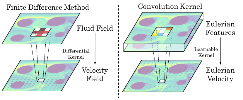
Based on the above idea, we capture the particle movement by the learnable convolutional layer $\operatorname{Conv}()$ based on the evolved deep Eulerian features $\tilde{\bm{x}}_{t+1}$:

$$\begin{split}\partial\mathbf{p}_{t}&=\operatorname{Interpolate}(\operatorname{Conv}(\tilde{\bm{x}}_{t+1}),\mathbf{p}_{t})\\ \mathbf{p}_{t+1}&=\mathbf{p}_{t}+\partial\mathbf{p}_{t},\end{split}$$ (12)

where the approximated velocity field of Eulerian features is interpolated to tracked particles. $\mathbf{p}_{t+1}$ denotes the moved particle position. In addition to the theoretical soundness, the above design can also benefit from the Eulerian features, which are better at presenting the shape of typical fluid phenomena, such as vortex or wake flow. For conciseness, the above process is simplified as $\operatorname{EuToLag}()$.

Overall, the EuLag block can fully utilize the complementary advantages of Eulerian and Lagrangian perspectives in describing fluid, thereby better apt at fluid prediction.

Figure 4: Showcases and timewise relative L2 on Bounded Naiver-Stokes dataset. Both predictions and absolute error maps are provided.

4 Experiments

We evaluated EuLagNet on three challenging datasets, including simulated and real-world scenarios, covering both 2D and 3D fluids. Following the previous work (Li et al., 2021), the task for each dataset is to predict 10 timesteps in an autoregressive fashion based on 10 past observations. Detailed categories of these datasets are listed in Table 1.

Table 1: Summary of experiment Datasets. #Var refers to the number of observed fluid quantities. #Space is the spatial resolution.

Datasets	Type	#Var	#Dim	#Space
Bounded N-S	Simulation	1	2D	$128\times 128$
Ocean Current	Real World	5	2D	$180\times 300$
3D Smoke	Simulation	4	3D	$32^{3}$

Baselines

To demonstrate the effectiveness of our model, we compare EuLagNet with six baselines on all benchmarks, including the classical deep model U-Net (2015) and advanced neural operators for Navier-Stokes equations: FNO (2021), Galerkin Transformer (2021), GNOT (2023), LSM (Wu et al., 2023) and FactFormer (Li et al., 2023). U-Net has been widely used in fluid modeling, which can model the multiscale property precisely. LSM (Wu et al., 2023) and FactFormer (Li et al., 2023) are previous state-of-the-art neural operators for fluid prediction.

Metrics

For all three datasets, we follow the convention in fluid prediction (Li et al., 2021; Wu et al., 2023) and report relative L2 as the main metric. For the real-world Ocean Current dataset, we also calculate the latitude-weighted Anomaly Correlation Coefficient (ACC) (Murphy & Epstein, 1989), which is commonly employed in earth science to evaluate the model prediction skill. It measures the correlation coefficient between anomalies in observations and predictions, indicating how accurately the model can forecast anomalous weather processes. The implementations of these metrics are included in Appendix B.3.

Implementations

Following the previous convention, EuLagNet is trained with relative L2 as the loss function on all three benchmarks. We use the Adam (Kingma & Ba, 2015) optimizer with an initial learning rate of $5\times 10^{-4}$ and cosine annealing learning rate scheduler. The batch size is set to 5, and the training process is stopped after 100 epochs. All experiments are implemented in PyTorch (Paszke et al., 2019) and conducted on a single NVIDIA A100 GPU.

4.1 Bounded Navier-Stokes

Setups

In real-world applications, it is important to handle complex boundary conditions in predicting fluid dynamics. Thus, we experiment with the newly generated Bounded Navier-Stokes. This benchmark simulates a scenario where some colored dye flows from left to right through a 2D pipe with several fixed pillars as obstacles inside. The motion of dye is simulated from the Navier-Stokes equation of incompressible fluid. 2000 sequences with spatial resolution of $128\times 128$ are generated for training and 200 new sequences are used for the test. Note that due to the pillars, the fluid dynamics are extremely intricate and will present the karman vortex street phenomena (Wille, 1960).

Quantitive results

As shown in Table 2, EuLagNet achieves the best performance in Bounded Navier-Stokes, demonstrating its advanced ability to handle complex boundary conditions. In comparison to the previous best model U-Net, EuLagNet achieves a significant 12.4% relative promotion (Relative L2: 0.0652 v.s. 0.0571). The timewise error curves of all the experiment models are also included in Figure 4. We can find that EuLagNet presents slower error growth and excels in long-term forecasting. This result may stem from the Lagrangian-guided fluid prediction, which can accurately capture the dynamics information over time, further verifying the effectiveness of our design.

Table 2: Performance comparison on the Bounded Naiver-Stokes dataset. Relative L2 is recorded. For clarity, the best result is in bold and the second best is underlined. Promotion represents the relative promotion of our model w.r.t the second best model.

Model	Relative L2
U-Net (Ronneberger et al., 2015)	0.0652
FNO (Li et al., 2021)	0.1153
Galerkin Transformer (Cao, 2021)	0.1125
GNOT (Hao et al., 2023)	0.1392
LSM (Wu et al., 2023)	0.0672
FactFormer (Li et al., 2023)	0.0733
EuLagNet (Ours)	0.0571
Promotion	12.4%

Showcases

To intuitively present the forecasting skills of different models, we also provide showcase comparisons in Figure 4. We can find that EuLagNet can precisely capture the vortex in the center of the figure as well as the Karmen vortex phenomenon formed behind the upper left pillar. As for U-Net and LSM, although they successfully predict the position of the center vortex, the error map presents that they fail to accurately predict the density of the flow field. In addition, FactFormer degenerates on this benchmark. This may come from that it is based on spatial factorization, which is unsuitable for irregularly placed boundary conditions. These results further highlight the benefits of Eulerian-Lagrangian co-design, which can help the dynamics and density prediction simultaneously.

Figure 5: Visualization sampling probability distribution (right) learned by EuLagNet. For a better view, we plot the $\log(\mathbf{S})$ here.

Learned sampling probability

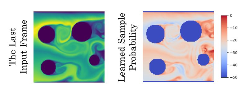
As we stated in Eq. (6), we adopt a learnable sampling strategy to capture the essential particles in the Eulerian space. To illustrate the effect of learnable probability, we visualize the learned distribution $\mathbf{S}$ in Figure 5. It is observed that the model tends to sample more on the regions with complex dynamics, such as the wake flow and Karmen vortex behind the pillar, demonstrating that our design in learnable probability can help the model track the most essential particles. Further, this design enables EuLagNet to capture vital Lagrangian dynamics as guidance, thereby boosting the final performance.

Figure 6: Showcase comparison and visualization of Lagrangian trajectories learned by EuLagNet on Ocean Current. Concretely, potential temperatures predicted from different models are plotted. Error maps of predictions are normalized to $(-4,4)$ for better visualization.

Table 3: Results on the Ocean Current dataset and the curve of timewise ACC. Both ACC averaged from 10 prediction steps and ACC of the last prediction frame are recorded. A higher ACC value indicates better performance. Relative promotion is also calculated.

Model	Relative L2	Avg. ACC	Last. ACC
U-Net (Ronneberger et al., 2015)	0.0373	0.0916	0.0888
FNO (Li et al., 2021)	0.0301	0.0883	0.0853
Galerkin Transformer (Cao, 2021)	0.0286	0.0896	0.0848
GNOT (Hao et al., 2023)	0.0215	0.4725	0.4557
LSM (Wu et al., 2023)	0.0202	0.2378	0.2305
FactFormer (Li et al., 2023)	0.0190	0.4789	0.4633
EuLagNet (Ours)	0.0172	0.4820	0.4694
Promotion	9.5%	0.6%	1.3%

4.2 Ocean Current

Setups

The prediction of ocean currents plays an important role in extensive areas, such as pollution abatement and new energy utilization. Thus, we also experiment with this valuable scenario. First, we downloaded daily sea reanalysis data (CMEMS & MDS, 2023) from 2011 to 2020 provided by the ECMWF and selected five basic variables on the sea surface to construct the dataset, including velocity, salinity, potential temperature, and height above the geoid. These variables are necessary to identify the ocean state. Then, we crop a $180\times 300$ sub-area on the North Pacific from the global record, corresponding to a 375km$\times$625km region. In total, this dataset consists of 3,653 frames, where the first 3000 frames are used for training and the last 653 frames are used for testing. This task is to predict the future current of 10 days based on the past 10 days’ observation.

Quantitive results

We report both relative L2 and ACC for the Ocean Current dataset in Table 4.1, where EuLagNet still achieves the best with 9.5% relative promotion w.r.t. the second-best model. These results demonstrate that EuLagNet performs well in real-world large-scale fluids. Different from simulated data, real-world records usually involve inherent stochasticity. Notably, EuLagNet also excels in the ACC metric, which can better quantify the model prediction skill. As shown in the timewise ACC curve, EuLagNet consistently achieves the highest ACC and holds more significant advantages in long-term prediction.

Showcases

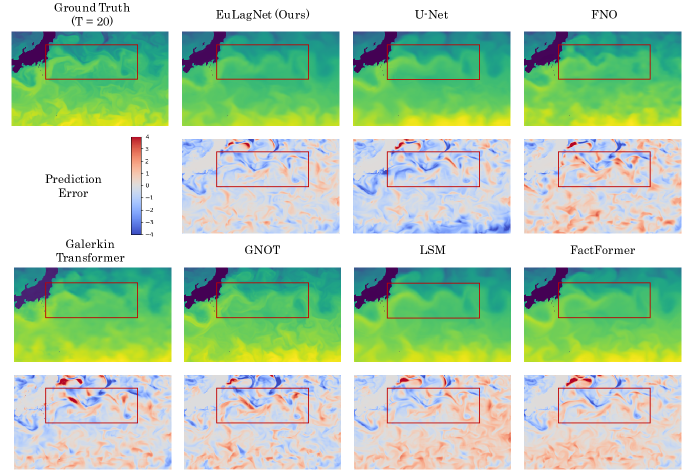
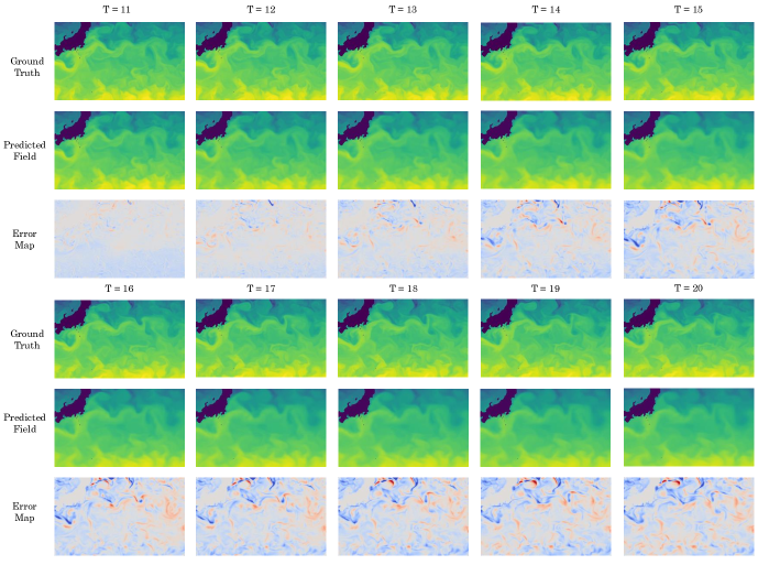
We presented a comparison of different model predictions in Figure 6. In comparison to other models, EuLagNet exhibits the smallest prediction error. It accurately predicts the location of the high-temperature region to the south area and provides a clear depiction of the Kuroshio pattern (Tang et al., 2000) bounded by the red box.

Learned trajectory visualization

To provide an intuitive illustration of the effect of learning Lagrangian trajectories, we also visualize tracked particles in Figure 6. We can find that all the particles learn to move from west to east, which matches the Pacific circulation. Furthermore, tracked particles exhibit distinct moving patterns, verifying their representation capability in complex dynamics. Especially, the movement of upper particles fits the sinuous trajectory of the Kuroshio current, indicating that EuLagNet can provide interpretable evidence for prediction results through visualizing tracking points in Lagrangian space.

4.3 3D Smoke

Setups

3D fluid prediction is a long-standing challenge due to high-dimensional tanglesome molecular interaction. To verify our model effectiveness in this complex setting, we also generate a 3D fluid dataset for the experiment. This benchmark consists of a scenario where smoke flows under the influence of buoyancy in a three-dimensional bounding box. This process is governed by the incompressible Navier-Stokes equation and the advection equation of fluid. 1000 sequences are generated for training and 200 new samples are used for test. Each case is in the resolution of $32^{3}$.

Table 4: Results on the 3D Smoke dataset. Relative L2 is recorded. “NaN” refers to the unstable training problem.

Model	Relative L2
U-Net (Ronneberger et al., 2015)	0.1431
FNO (Li et al., 2021)	0.0648
Galerkin Transformer (Cao, 2021)	NaN
GNOT (Hao et al., 2023)	0.2152
LSM (Wu et al., 2023)	0.0634
FactFormer (Li et al., 2023)	0.0784
EuLagNet (Ours)	0.0591
Promotion	6.8%

Figure 7: Showcases comparison of the whole space (left part) and a cross-section (right part) on 3D Smoke Dataset. For better visualization, we present the absolute value of the prediction error and normalize the whole space error into $(0,0.12)$. As for the cross-section visualization, we choose the $xOy$ plane in the middle 3D fluid and normalize error maps to $(-0.5,0.5)$.

Quantitive results

Table 4 presents that EuLagNet still achieves the best performance in 3D fluid simulation. Note that in this benchmark, the canonical deep model U-Net degenerates seriously, indicating that a pure multiscale framework is insufficient to model complex dynamics. Besides, we also notice that the Transformer-based neural operators, such as GNOT and Galerkin Transformer, also fail in this task. This is because both of them are based on the linear attention mechanism (Kitaev et al., 2020; Xiong et al., 2021), which may degenerate under massive tokens. These comparisons further highlight the capability of EuLagNet in handling high-dimensional fluid and intricate dynamics.

Showcases

In Figure 7, we present a comparison of prediction results on the smoke dataset. EuLagNet performs well in capturing the convection and diffusion of smoke within the bounding box. In comparison, the predictions from U-Net tend to predict the averaged value across various surfaces, resulting in blurred details, which also indicates its deficiency in dynamics modeling. As for LSM and FactFormer, we can find that they present more errors in the smoke boundaries that usually involve complex waves. In contrast, our model excels in both overall and cross-section error and performs excellent in predicting subtle flows.

4.4 Model Analysis

Table 5: Ablations on Bounded Naiver-Stokes, including reducing tracking particles of the first layer ($M_{1}$), removing Lagrangian-guided feature evolving $\operatorname{LagToEu}()$, Eulerian-conditioned particle tracking $\operatorname{EuToLag}()$ and learnable particle sampling strategy.

Design	Relative L2	Decrease
EuLagNet ($M_{1}=512$)	0.0571	-
$M_{1}=128$	0.0599	-4.9%
$M_{1}=256$	0.0592	-3.7%
$M_{1}=768$	0.0573	-0.3%
w/o $\operatorname{LagToEu}()$	0.0676	-18.4%
w/o $\operatorname{EuToLag}()$	0.0663	-16.1%
w/o Learnable Sampling	0.0584	-2.3%

Ablations

To verify the effectiveness of every detailed design in EuLagNet, we conduct exhaustive ablations in Table 5. In our original design, we track 512 particles (around 3% of Eulerian grids). The experiments show that increasing the number of particles will boost the model performance, which means more fine-grained dynamics tracking. Thus, we choose $M_{1}=512$ to balance efficiency and performance. In addition, we can conclude that all components proposed in this paper are indispensable. Especially, the lack of interaction between the Eulerian and Lagrangian space will cause a serious drop in accuracy, highlighting the importance of dual cross-attention. Besides, rather than uniformly sampling particles, sampling from a learnable probability matrix also provides a promotion. The above results provide solid support to our motivation in tracking essential particles and utilizing Eulerian-Lagrangian dual recurrence, further confirming the merits of our model.

Efficiency analysis

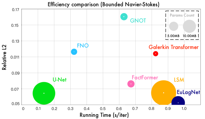
We also include the efficiency comparison in Figure 8. Considering performance, model parameters and running time simultaneously, EuLagNet achieves a favorable trade-off between efficiency and performance. Note that although U-Net is good at Bounded Naiver-Stokes, it will degenerate seriously when it comes to complex fluid dynamics, such as Ocean Current and 3D Smoke.

Figure 8: Efficiency comparison among all the models. Running time and Relative L2 are evaluated on the Bounded Navier-Stokes.

5 Conclusions

To tackle intricate fluid dynamics, this paper presents EuLagNet by introducing the Lagrangian dynamics into Eulerian fluid, which can provide clear and neat dynamics information for prediction. A EuLag block is presented in the Eulerian-Lagrangian Dual Recurrent Network to utilize the complementary advantages of Eulerian and Lagrangian perspectives, which brings better particle tracking and Eulerian fluid prediction. EuLagNet excels in complex fluid prediction, even in 3D fluid, and can also provide interpretable evidence by plotting learned Lagrangian trajectories.

Appendix A Physical Insights for Eulerian-Conditioned Particle Tracking

As we stated in Figure 3, tracking particles in the EuLag block is inspired by the traditional numerical method Finite Difference Method (FDM). In this section, we elaborate on the physical insights of our design and show how the learnable convolution kernel in EuLagNet for updating position can represent learning the fluid velocity field in FDM.

The fluids in the real world are commonly governed by a complex system of partial differential equations (PDEs), for instance, the Naiver-Stokes equations. However, in most cases, these partial differential equations (PDEs) lack analytical solutions and can only be approximated through various numerical methods (Temam, 2001). Due to its convenient representation and simple computation, FDM is an outstanding and common method among such numerical methods (Ferziger et al., 2020). By discretizing the solution space onto a regular grid, FDM utilizes numerical derivatives derived from Taylor expansions to replace the differential operators in partial differential equations (PDEs) (Mitchell & Griffiths, 1980). Afterward, FDM approximates the exact solution at grid points through iterative calculations.

Specifically, for a two-dimensional Eulerian representation dataset of a fluid PDE defined on a bounded domain $\mathcal{D}$ in the $x$-$y$ plane, the observation intervals $\Delta x$ and $\Delta y$ along the $x$ and $y$ axes, respectively, represent the spatial steps in FDM. The time interval $\Delta t$ between consecutive frames corresponds to the temporal step in FDM.

As a supplement to Section 3.2, we consider a pertinent example closely related to our task, that is the 2D Naiver-Stokes equation within $\mathcal{D}=\{(x,y,t)|0\leq x,y\leq 1,t\geq 0\}$ (White, 2011) :

$$\dfrac{\partial\bm{u}}{\partial t}+(\bm{u}\cdot\nabla)\bm{u}=-\dfrac{1}{\rho}\nabla p+\nu\nabla^{2}\bm{u}.$$ (13)

Here, $\bm{u}=(u,v)$ denotes the flow velocity, which is a vector function of $(x,y,t)$. $p$ is the pressure. For simplicity, we assume the fluid is isotropic and incompressible, which means the density $\rho$ and dynamic viscosity $\nu$ are constant in $\mathcal{D}$.

In FDM, given the origin $(0,0,0)$, all the partial differential terms in a PDE at $(x_{i},y_{j},t_{k})=(i\Delta x,j\Delta y,k\Delta t)$ can be approximated by a discrete equation based on the difference scheme. If we utilize central explicit scheme (Mitchell & Griffiths, 1980; Toro, 2009), we can obtain the following approximation:

$$\frac{\partial\bm{u}}{\partial t}\approx \frac{\bm{u}_{i,j}^{k+1}-\bm{u}_{i,j}^{k}}{\Delta t}$$ (14)

$$(\bm{u}\cdot\nabla)\bm{u}\approx \left(\frac{u_{i+1,j}^{k}-u_{i-1,j}^{k}}{2\Delta x},\frac{v_{i,j+1}^{k}-v_{i,j-1}^{k}}{2\Delta y}\right)$$

$$\frac{\partial p}{\partial x}\approx \frac{p_{i+1,j}^{k}-p_{i-1,j}^{k}}{2\Delta x},\ \ \frac{\partial p}{\partial y}\approx\frac{p_{i,j+1}^{k}-p_{i,j-1}^{k}}{2\Delta y}$$

$$\nabla^{2}\bm{u}\approx \left(\frac{u_{i+1,j}^{k}-2u_{i,j}^{k}+u_{i-1,j}^{k}}{\Delta x^{2}},\frac{v_{i,j+1}^{k}-2v_{i,j}^{k}+v_{i,j-1}^{k}}{\Delta y^{2}}\right).$$

Here, $\bm{u}_{i,j}^{k}$ represents the approximate value of $\bm{u}(x_{i},y_{j},t_{k})$. Substituting the left-hand-side terms in Eq. (13) with their right-hand-side approximation in Eq. (14), we can calculate an unknown quantity by its known neighbors and the initial condition. For $\frac{\partial\bm{u}}{\partial t}$ that we are interested in, it is:

$$\frac{\bm{u}_{i,j}^{k+1}-\bm{u}_{i,j}^{k}}{\Delta t}=\mathbf{K}\odot\begin{bmatrix}\bm{u}_{i-1,j+1}^{k}&\bm{u}_{i,j+1}^{k}&\bm{u}_{i+1,j+1}^{k}\\ \bm{u}_{i-1,j}^{k}&\bm{u}_{i,j}^{k}&\bm{u}_{i+1,j}^{k}\\ \bm{u}_{i-1,j-1}^{k}&\bm{u}_{i,j-1}^{k}&\bm{u}_{i+1,j-1}^{k}\\ \end{bmatrix},$$ (15)

where $\odot$ represents the element-wise product. Eq. (15) is referred to as the (finite) difference equation of $\bm{u}$ approximating the original continuous PDEs (Eq. (13)), where $\mathbf{K}$ depends on the variable we investigate and the choice of the difference scheme. In the central explicit scheme (Mitchell & Griffiths, 1980; Toro, 2009), $\mathbf{K}$ is given by:

$$\mathbf{K}=\begin{bmatrix}0&\frac{2\nu-\Delta y}{2\Delta y^{2}}+r_{1}(p_{i,j+1}^{n})&0\\ \frac{2\nu+\Delta x}{2\Delta x^{2}}+r_{2}(p_{i-1,j}^{n})&\frac{-2\nu(\Delta x+\Delta y)}{\Delta x^{2}\Delta y^{2}}+r_{3}(p_{i,j}^{n})&\frac{2\nu-\Delta x}{2\Delta x^{2}}+r_{4}(p_{i+1,j}^{n})\\ 0&\frac{2\nu+\Delta y}{2\Delta y^{2}}+r_{5}(p_{i,j-1}^{n})&0\\ \end{bmatrix}.$$ (16)

Where $r_{i},\ i\in\{1,\dots,5\}$ are functions of pressure value.

We can notice that Eq. (15) is identical to a convolution operation with kernel $\mathbf{K}$. Recall the task stated in Eulerian-Conditioned Particle Tracking, the object of the learnable convolutional layer $\operatorname{Conv}()$ is to extract the dynamics from the current Eulerian fluid, in other words, solving a finite difference scheme of the current fluid field by learning the convolutional kernel to determine the optimal difference scheme. Thus, the learnable convolution kernel in EuLagNet for updating position can represent learning the fluid velocity field in FDM.

Appendix B Implementation Details

In this section, we provide the implementation details of EuLagNet, including the configurations of model hyperparameters and the concrete design of modules.

B.1 Hyperparameters

Detailed model configurations of EuLagNet are listed in Table 6. Zero-padding is only used in the Ocean Current dataset to ensure the exact division in downsampling.

Table 6: Model configurations for EuLagNet.

Model Designs	Hyperparameters	Values
	Number of observation steps $P$	$10$
	Number of scales $L$	$4$
Eulerian-Lagrangian	Sample Points at each scale $\{M_{1},\cdots,M_{L}\}$	$\{512,128,32,8\}$
Dual Recurrent Network	Downsample Ratio $r=\frac{|\mathcal{D}_{l+1}|}{|\mathcal{D}_{l}|}$	$0.5$
	Channels of each scale $\{C_{1},\cdots,C_{L}\}$	$\{64,128,256,256\}$
	Paddings for Ocean Current Dataset	$(12,20)$
	Heads in Dual Cross-Attention	8
EuLag Block	Channels per head in Dual Cross-Attention	64
	Kernel Size in the Learnable Convolutional Layer	3

B.2 Multiscale architecture

Encoder

Given Eulerian fluid functions $\{\tilde{\bm{x}}_{t}(\mathbf{s})\}_{\mathbf{s}\in\mathcal{D}}$ at the $t$-th time step and $\{\tilde{\bm{x}}_{(t-P+1):(t-1)}(\mathbf{s})\}_{\mathbf{s}\in\mathcal{D}}$ at previous time steps, the $\operatorname{Encode}()$ operation is to project original fluid properties in physical domain to deep representations with linear layer and position embedding, which can be formalized as follows:

$$\begin{split}\displaystyle\tilde{\bm{x}}_{t}^{1}=\operatorname{Linear}\Big{(}\operatorname{Concat}\big{(}\{\tilde{\bm{x}}_{(t-P+1):t}(\mathbf{s})\}_{\mathbf{s}\in\mathcal{D}}\big{)}\Big{)}+\operatorname{PosEmbedding}.\\ \end{split}$$ (17)

Decoder

Given evolved Eulerian deep representations in the finest scale $\{\tilde{\bm{x}}_{t+1}^{1}(\mathbf{s})\}_{\mathbf{s}\in\mathcal{D}}$ at the $(t+1)$-th time step, the $\operatorname{Decode}()$ operation is to project deep representations back to predicted fluid properties with two linear layers and a $\operatorname{GeLU}$ activation (Hendrycks & Gimpel, 2016), which can be formalized as follows:

$$\begin{split}\displaystyle\tilde{\bm{x}}_{t+1}=\operatorname{Linear}\Big{(}\operatorname{GeLU}\big{(}\operatorname{Linear}(\{\tilde{\bm{x}}_{t+1}^{1}(\mathbf{s})\}_{\mathbf{s}\in\mathcal{D}})\big{)}\Big{)}.\\ \end{split}$$ (18)

$\mathbf{Conv()}$ in Particle Movement

Given the evolved Eulerian deep representations $\{\tilde{\bm{x}}_{t+1}^{l}(\mathbf{s})\}_{\mathbf{s}\in\mathcal{D}_{l}}$ outputted by the dual cross-attention at the $l$-th scale, the $\operatorname{Conv}()$ operation in Eq. (12) is to extract the dynamics of particles from the deep representations with $\operatorname{Conv}()$, $\operatorname{BatchNorm}()$ and $\operatorname{ReLU}()$ layers, which can be formalized as follows:

$$\begin{split}\displaystyle\frac{\partial\bm{x}_{t}^{l}}{\partial t}=\operatorname{Conv}\Bigg{(}\operatorname{ReLU}\Big{(}\operatorname{BatchNorm}\big{(}\operatorname{Conv}(\{\tilde{\bm{x}}_{t+1}^{l}(\mathbf{s})\}_{\mathbf{s}\in\mathcal{D}_{l}})\big{)}\Big{)}\Bigg{)},\ \text{$l$ from $1$ to $L$}.\end{split}$$ (19)

Then, the dynamics of the tracking particles are obtained by interpolation:

$$\begin{split}\displaystyle\frac{\partial\mathbf{p}_{t}^{l}}{\partial t}=\operatorname{Interpolate}(\frac{\partial\bm{x}_{t}^{l}}{\partial t},\mathbf{p}_{t}),\ \text{$l$ from $1$ to $L$}.\end{split}$$ (20)

Finally, the position of moved particles $\mathbf{p}_{t+1}^{l}$ is accumulated by:

$$\begin{split}\displaystyle\mathbf{p}_{t+1}^{l}=\mathbf{p}_{t}^{l}+\frac{\partial\mathbf{p}_{t}^{l}}{\partial t},\ \text{$l$ from $1$ to $L$}.\end{split}$$ (21)

Downsample

Given Eulerian deep representations $\{\tilde{\bm{x}}_{t}^{l}(\mathbf{s})\}_{\mathbf{s}\in\mathcal{D}_{l}}$ at the $l$-th scale, the $\operatorname{Down}()$ operation is to concentrate local information of deep representations into a smaller feature map at the $(l+1)$-th scale with $\operatorname{MaxPooling}()$ and $\operatorname{Conv}()$ layers, which can be formalized as follows:

$$\begin{split}\displaystyle\tilde{\bm{x}}_{t}^{l+1}=\operatorname{Conv}\Big{(}\operatorname{MaxPooling}\big{(}\{\tilde{\bm{x}}_{t}^{l}(\mathbf{s})\}_{\mathbf{s}\in\mathcal{D}_{l}}\big{)}\Big{)},\ \text{$l$ from $1$ to $(L-1)$}.\end{split}$$ (22)

Upsample

Given the evolved Eulerian deep representations $\{\tilde{\bm{x}}_{t+1}^{l}(\mathbf{s})\}_{\mathbf{s}\in\mathcal{D}_{l}}$ at the $l$-th scale and $\{\tilde{\bm{x}}_{t+1}^{l+1}(\mathbf{s})\}_{\mathbf{s}\in\mathcal{D}_{l+1}}$ at the $(l+1)$-th scale, respectively, the $\operatorname{Up}()$ operation is to fuse information on corresponding position between two adjacent scales of deep representations into a feature map at the $l$-th scale with $\operatorname{Interpolate}()$ operation and $\operatorname{Conv}()$ layers, which can be formalized as follows:

$$\begin{split}\displaystyle\tilde{\bm{x}}_{t+1}^{l}=\operatorname{Conv}\Bigg{(}\operatorname{Concat}\Big{(}\Big{[}\operatorname{Interpolate}\big{(}\{\tilde{\bm{x}}_{t+1}^{l+1}(\mathbf{s})\}_{\mathbf{s}\in\mathcal{D}_{l+1}}\big{)},\{\tilde{\bm{x}}_{t+1}^{l}(\mathbf{s})\}_{\mathbf{s}\in\mathcal{D}_{l}}\Big{]}\Big{)}\Bigg{)},\ \text{$l$ from $(L-1)$ to $1$}\end{split}$$ (23)

B.3 Metrics

Relative L2

For all three datasets, we use the relative L2 as the primary metric. Compared to MSE, Relative L2 is less influenced by outliers and is, therefore, more robust. For given $n$ steps 2D predictions $\hat{\mathbf{x}}\in\mathbb{R}^{H\times W\times n}$ or 3D predictions $\hat{\mathbf{x}}\in\mathbb{R}^{H\times W\times C\times n}$ and their corresponding ground truth $\mathbf{x}$ of the same size, the relative L2 can be expressed as:

$$\operatorname{Relative~{}L2}=\frac{\|\mathbf{x}-\hat{\mathbf{x}}\|_{2}^{2}}{\|\mathbf{x}\|_{2}^{2}},$$ (24)

where $\|\cdot\|_{2}$ represents the L2 norm.

Latitude-weighted Anomaly Correlation Coefficient

In meteorology, directly calculating the correlation between predictions and ground truth may obtain misleadingly high values because of the seasonal variations. To subtract the climate average from both the forecast and the ground truth, we utilize the Anomaly Correlation Coefficient to verify the forecast and observations. Moreover, since the observation grids are equally spaced in latitude, the size of the different grids is related to the latitude and thus, we calculate the latitude-weighted Anomaly Correlation Coefficient, which can be formalized as:

$$\operatorname{ACC}(v,t)=\frac{\sum_{i,j}\text{Lat}(\phi_{i})\hat{\mathbf{x}}_{i,j,t}^{\prime v}\mathbf{x}_{i,j,t}^{\prime v}}{\sqrt{\sum_{i,j}\text{Lat}(\phi_{i})\left(\hat{\mathbf{x}}_{i,j,t}^{\prime v}\right)^{2}\times\sum_{i,j}\text{Lat}(\phi_{i})\left(\mathbf{x}_{i,j,t}^{\prime v}\right)^{2}}},$$ (25)

where $v$ represents a certain observed variable, $\hat{\mathbf{x}}_{i,j,t}$ is the prediction of ground truth $\mathbf{x}$ at position $i,j$ and forecast time $t$. $\mathbf{x}^{\prime}=\mathbf{x}-\bar{\mathbf{x}}$ represents the difference between $\mathbf{x}$ and the climatology $\bar{\mathbf{x}}$, that is, the long-term mean of observations in the dataset. $\text{Lat}(\phi_{i})=N_{\text{Lat }}\times\frac{\cos\phi_{i}}{\sum_{i^{\prime}=1}^{N_{\text{Lat }}}\cos\phi_{i^{\prime}}}$, where $N_{\text{Lat}}=180$ and $\phi_{i}$ is the latitude of the $i$-th row of output.

Appendix C Training Curves

Figure 9: Training curve comparison among all the models on Bounded Naiver-Stokes dataset, Ocean Current, and 3D Smoke dataset.

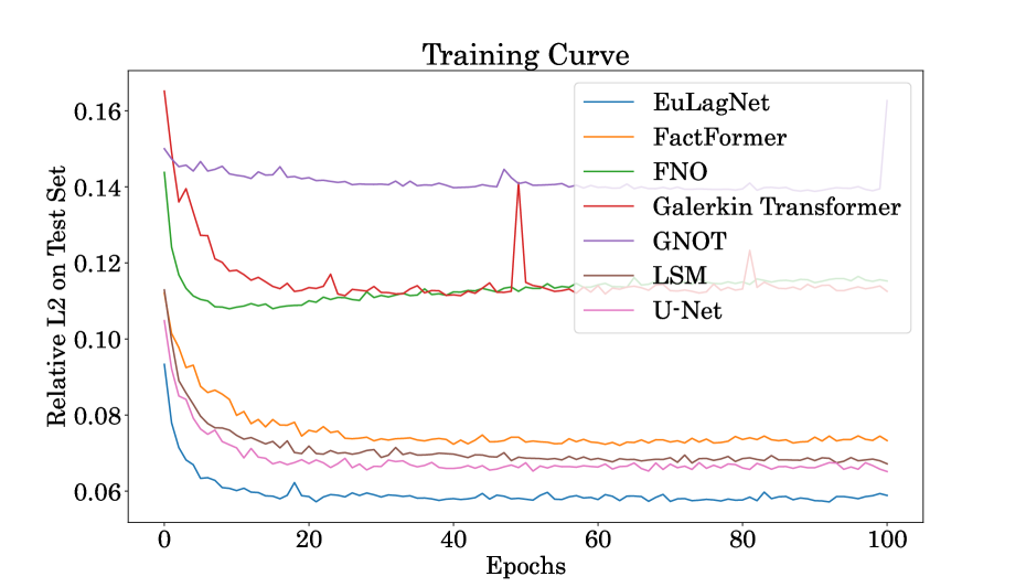
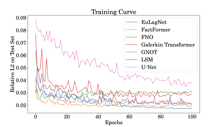
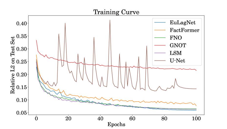
We provide training curves on Bounded Navier-Stokes, Ocean Current and 3D Smoke datasets in Figure 9. We can observe that EuLagNet presents favorable training robustness and converges the fastest on the Bounded Navier-Stokes dataset.

Appendix D More Showcases

As a supplement to the main text, we provide more showcases here for comparison (Figure 10-14).

Figure 10: Showcases of the Bounded Navier-Stokes dataset.

Figure 11: Showcases of EuLagNet on the Bounded Navier-Stokes dataset.

Figure 12: Showcases of the 3D Smoke dataset.

Figure 13: Showcases of EuLagNet on the 3D Smoke dataset.

Figure 14: Showcases of the Ocean Current dataset.

Figure 15: Showcases of EuLagNet on the Ocean Current dataset.

References

- Cao (2021) Cao, S. Choose a transformer: Fourier or galerkin. In Conference on Neural Information Processing Systems, 2021.
- CMEMS & MDS (2023) CMEMS and MDS. Global ocean physics reanalysis. DOI: 10.48670/moi-00021 (Accessed on 23 September 2023), 2023.
- Dissanayake & Phan-Thien (1994) Dissanayake, M. and Phan-Thien, N. Neural-network-based approximations for solving partial differential equations. Communications in Numerical Methods in Engineering, 1994.
- Dong et al. (2017) Dong, B., Jiang, Q., and Shen, Z. Image restoration: Wavelet frame shrinkage, nonlinear evolution pdes, and beyond. Multiscale Modeling & Simulation, 2017.
- Ferziger et al. (2020) Ferziger, J., Perić, M., and Street, R. Computational Methods for Fluid Dynamics. Springer Nature Switzerland, 2020.
- Fornberg (1998) Fornberg, B. A practical guide to pseudospectral methods. Cambridge university press, 1998.
- Gupta (1988) Gupta, K. Classical Mechanics of Particles and Rigid Bodies. Wiley, 1988.
- Hao et al. (2023) Hao, Z., Ying, C., Wang, Z., Su, H., Dong, Y., Liu, S., Cheng, Z., Zhu, J., and Song, J. Gnot: A general neural operator transformer for operator learning. In International Conference on Machine Learning, 2023.
- Hendrycks & Gimpel (2016) Hendrycks, D. and Gimpel, K. Gaussian error linear units (gelus). arXiv: Learning, 2016.
- Kingma & Ba (2015) Kingma, D. P. and Ba, J. Adam: A method for stochastic optimization. In International Conference on Learning Representations, 2015.
- Kitaev et al. (2020) Kitaev, N., Kaiser, L., and Levskaya, A. Reformer: The efficient transformer. In International Conference on Learning Representations, 2020.
- Li et al. (2021) Li, Z., Kovachki, N. B., Azizzadenesheli, K., liu, B., Bhattacharya, K., Stuart, A., and Anandkumar, A. Fourier neural operator for parametric partial differential equations. In International Conference on Learning Representations, 2021.
- Li et al. (2022) Li, Z., Huang, D. Z., Liu, B., and Anandkumar, A. Fourier neural operator with learned deformations for pdes on general geometries. arXiv preprint, 2022.
- Li et al. (2023) Li, Z., Shu, D., and Farimani, A. B. Scalable transformer for pde surrogate modeling. In Conference on Neural Information Processing Systems, 2023.
- Lu et al. (2021) Lu, L., Jin, P., Pang, G., Zhang, Z., and Karniadakis, G. E. Learning nonlinear operators via deeponet based on the universal approximation theorem of operators. Nature Machine Intelligence, 2021.
- Mitchell & Griffiths (1980) Mitchell, A. and Griffiths, D. The Finite Difference Method in Partial Differential Equations. 1980.
- Murphy & Epstein (1989) Murphy, A. H. and Epstein, E. S. Skill scores and correlation coefficients in model verification. Monthly weather review, 1989.
- Paszke et al. (2019) Paszke, A., Gross, S., Massa, F., Lerer, A., Bradbury, J., Chanan, G., Killeen, T., Lin, Z., Gimelshein, N., Antiga, L., et al. Pytorch: An imperative style, high-performance deep learning library. Advances in Neural Information Processing Systems, 2019.
- Raissi et al. (2017) Raissi, M., Perdikaris, P., and Karniadakis, G. E. Physics informed deep learning (part i): Data-driven solutions of nonlinear partial differential equations. arXiv preprint, 2017.
- Raissi et al. (2019) Raissi, M., Perdikaris, P., and Karniadakis, G. E. Physics-informed neural networks: A deep learning framework for solving forward and inverse problems involving nonlinear partial differential equations. Journal of Computational Physics, 2019.
- Ronneberger et al. (2015) Ronneberger, O., Fischer, P., and Brox, T. U-net: Convolutional networks for biomedical image segmentation. In The Medical Image Computing and Computer Assisted Intervention Society, 2015.
- Ruthotto & Haber (2018) Ruthotto, L. and Haber, E. Deep neural networks motivated by partial differential equations. Journal of Mathematical Imaging and Vision, 2018.
- Sim et al. (2021) Sim, F., Budiarto, E., and Rusyadi, R. Comparison and analysis of neural solver methods for differential equations in physical systems. ELKHA: Jurnal Teknik Elektro, 2021.
- Tang et al. (2000) Tang, T., Tai, J., and Yang, Y. The flow pattern north of taiwan and the migration of the kuroshio. Continental Shelf Research, 2000.
- Temam (2001) Temam, R. Navier-Stokes equations: theory and numerical analysis. American Mathematical Soc., 2001.
- Toro (2009) Toro, E. Riemann Solvers and Numerical Methods for Fluid Dynamics: A Practical Introduction. 2009.
- Trunk (1979) Trunk, G. V. A problem of dimensionality: A simple example. IEEE Transactions on Pattern Analysis and Machine Intelligence, 1979.
- Umetani & Bickel (2018) Umetani, N. and Bickel, B. Learning three-dimensional flow for interactive aerodynamic design. ACM Transactions on Graphics (TOG), 2018.
- Wang et al. (2023) Wang, H., Fu, T., Du, Y., Gao, W., Huang, K., Liu, Z., Chandak, P., Liu, S., Van Katwyk, P., Deac, A., et al. Scientific discovery in the age of artificial intelligence. Nature, 2023.
- Wang et al. (2020a) Wang, S., Teng, Y., and Perdikaris, P. Understanding and mitigating gradient pathologies in physics-informed neural networks. SIAM Journal on Scientific Computing, 2020a.
- Wang et al. (2020b) Wang, S., Yu, X., and Perdikaris, P. When and why pinns fail to train: A neural tangent kernel perspective. Journal of Computational PhysicsF, 2020b.
- Weinan & Yu (2017) Weinan, E. and Yu, T. The deep ritz method: A deep learning-based numerical algorithm for solving variational problems. Communications in Mathematics and Statistics, 2017.
- White (2011) White, F. Fluid Mechanics. McGraw-Hill series in mechanical engineering. 2011.
- Wille (1960) Wille, R. Karman vortex streets. Advances in Applied Mechanics, 1960.
- Wu et al. (2023) Wu, H., Hu, T., Luo, H., Wang, J., and Long, M. Solving high-dimensional pdes with latent spectral models. In International Conference on Machine Learning, 2023.
- Xiong et al. (2021) Xiong, Y., Zeng, Z., Chakraborty, R., Tan, M., Fung, G. M., Li, Y., and Singh, V. Nyströmformer: A nyström-based algorithm for approximating self-attention. Proceedings of the AAAI Conference on Artificial Intelligence, 2021.