DeLLMa: A Framework for Decision Making Under Uncertainty
with Large Language Models

Abstract

Large language models (LLMs) are increasingly used across society, including in domains like business, engineering, and medicine. These fields often grapple with decision-making under uncertainty, a critical yet challenging task. In this paper, we show that directly prompting LLMs on these types of decision-making problems yields poor results, especially as the problem complexity increases. To overcome this limitation, we propose DeLLMa (Decision-making Large Language Model assistant), a framework designed to enhance decision-making accuracy in uncertain environments. DeLLMa involves a multi-step scaffolding procedure, drawing upon principles from decision theory and utility theory, to provide an optimal and human-auditable decision-making process. We validate our framework on decision-making environments involving real agriculture and finance data. Our results show that DeLLMa can significantly improve LLM decision-making performance, achieving up to a 40% increase in accuracy over competing methods.

[Deqing]dfblue [Oliver]olorange L1/.style=draw=black,, L2/.style=,edge=,line width=0.8pt,

University of Southern California

1 Introduction

Large language models (LLMs) are rapidly gaining traction across many domains due to their potential for automating and enhancing a broad spectrum of tasks (Bommasani et al., 2021; Bubeck et al., 2023). One important potential use is in decision making under uncertainty, i.e., providing guidance on what action to take, given some set of possibilities, properly factoring in user goals and uncertainty about the world. The ability to make good decisions under uncertainty holds broad relevance across high-stakes tasks in fields such as business, marketing, medicine, aeronautics, and logistics (Kochenderfer, 2015; Peterson, 2017)—and its value is not limited to organization or company-level decisions but extends to aiding individuals in making informed choices as well. The ability of LLMs to analyze large quantities of data makes them potentially well-suited for sophisticated decision support tools, and ensuring that these models give accurate, context-aware recommendations could significantly augment human decision-making capabilities.

Figure 1: Given a decision query from a user, our framework DeLLMa (Decision-making LLM assistant) aims to perform optimal decision making under uncertainty. We illustrate DeLLMa on two decision-making tasks: agriculture (left) and stocks (right).

However, optimal decision making under uncertainty is difficult—even for humans. There exist frameworks from decision theory and utility theory (developed in fields such as economics, statistics, and philosophy) to provide humans with a structured approach for more rational and optimal decision-making (Von Neumann & Morgenstern, 1944; Luce & Raiffa, 1989; Berger, 2013). Research has consistently demonstrated that without these frameworks, human decision-making can often be highly irrational, swayed by biases and incomplete information (Bazerman & Moore, 2012). Similarly, achieving optimal decisions with LLMs presents its own set of difficulties. Issues include the tendency to fixate on specific explanations or information without adequately balancing all evidence, and inability to effectively handle uncertainty, manage biases, or align with a user’s goals and utilities (Ferrara, 2023; Benary et al., 2023). Our paper presents experiments that exemplify these issues.

Furthermore, beyond merely making optimal decisions, it is crucial to understand why an LLM made a particular decision. This understanding aids in building trust in the decision, verifying its optimality, and improving any components that may lead to suboptimal outcomes. The ability to explain decisions and verify decision-making quality—a concept we refer to as human auditability—is essential for the practical application of LLMs to aid decision making in many real problems (Thirunavukarasu et al., 2023).

In this paper, our goal is to develop a framework that enables LLMs to make more-optimal decisions under uncertainty. This framework is designed not only to enhance decision-making accuracy but also to allow human users to understand the rationale behind each decision and evaluate its optimality. Drawing inspiration from prior work on multi-step scaffolding like Chain of Thought (CoT) (Wei et al., 2022) and Tree of Thoughts (ToT) (Yao et al., 2023), we provide a scaffold for LLMs, which follows the framework of classical decision theory, originally designed for optimal decision making under uncertainty by humans. Our approach involves several key steps: first, identifying and forecasting pertinent unknown variables given in-context information; second, eliciting a utility function that aligns with the user’s goals; and finally, using this utility function to identify the decision that maximizes expected utility. We call our proposed framework DeLLMa, short for Decision-making Large Language Model assistant.

After introducing our framework, we show results on benchmark decision-making environments involving real datasets. These environments are designed to simulate two realistic decision-making scenarios: one in agriculture and another in finance. We then conduct a comparative analysis of DeLLMa against various LLM decision-making strategies, including zero-shot (direct) prompting, self-consistency (Wang et al., 2022), and CoT approaches. Our findings indicate that DeLLMa significantly enhances decision-making accuracy, with improvements of up to a (XYZ)%40% increase in prediction accuracy in both scenarios, particularly noticeable as the complexity and number of potential actions increases. Additionally, DeLLMa’s structure allows us to understand the rationale behind each decision it makes. In full, our contributions are:

• We introduce DeLLMa, a framework for optimal, human-auditabile LLM-based decision making under uncertainty, employing a multi-step scaffolding procedure.

• We detail and implement a specific version of this framework, tailored to address a subset of decision problems, which is compatible with current LLMs.

• On multiple realistic decision-making environments, we show that DeLLMa gives up to a (XYZ)%40% improvement in optimal decision-making accuracy over competing methods.

2 Related Work

Decision Making with LLMs.

Initiated by Chain-of-Thought (CoT) prompting (Wei et al., 2022), a plethora of recent works have developed frameworks to decompose complex, multi-step reasoning problems—including decision-making—into modular sub-problems. For example, Tree-of-Thought (ToT) prompting (Yao et al., 2023) generalizes CoT with a tree-search procedure to optimize a reasoning path subject to external feedback. Subsequent works aim to improve ToT with better search algorithms, self-induced feedback, and tool usage (Hao et al., 2023; Qin et al., 2023a; Zhuang et al., 2023; Ye et al., 2023).

However, none of these existing works focus on a framework for decision-making under uncertainty, which we demonstrate is challenging even for carefully-crafted chains that emulate classical decision-making procedures.

Another line of work leverages LLMs for optimizing blackbox functions (Yang et al., 2023; Nie et al., 2023; Shinn et al., 2023). These settings involve methods that make a substantial number of low-cost decisions (which do not incur a high price for suboptimality). Instead, we focus on single-step expensive decisions, particularly in the prescence of uncertainty, with a focus on the optimality of decisions.

Additionally, a number of applied domains that involve decision making have recently started to explore using LLM-based methods, such as in supply chain optimization (Li et al., 2023), and automated driving (Mao et al., 2023).

Uncertainty with LLMs.

LLMs, without proper calibration, can be overly confident in their responses (Si et al., 2022). Such pitfalls make them unlikely to make reliable decisions under uncertainty. Prior work has aimed to solve this issue; one line of research involves asking LLMs for their own confidence, with or without additional finetuning (Kadavath et al., 2022; Lin et al., 2022; Mielke et al., 2022; Chen & Mueller, 2023). Such methods can be costly if finetuning is needed or can perform poorly when an overconfident model attempts to evaluate its own confidence. Lin et al. (2023) propose an alternative uncertainty quantification method through selective NLG. Similar approaches are also used in LLM tool-usage literature (Ren et al., 2023).

3 Methods

Preliminaries

Suppose that a decision maker needs to make a choice between a set of options to achieve some goal—we refer to this as a decision problem. We begin by formalizing a decision problem, and afterwards describe how we approach decision making with LLMs. There are three main components to the decision problems that we will describe: actions, states, and utilities.

First, the actions are the possible options that a decision maker wishes to choose between. We use $\mathcal{A}$ to denote the space of actions, and $a\in\mathcal{A}$ for a single action in this set.

The second main component is the set of unknown states of nature, denoted $\Theta$. In our formulation, we define a state $\theta\in\Theta$ to be any latent variable whose true value is unknown, yet affects outcomes relevant to the decision maker’s goals. To perform optimal decision making, one must act while accounting for uncertainty over these unknown states.

Third, an important component is the decision maker’s preferences for different possible outcomes. We formalize our framework for decision making under uncertainty using utility theory, which can be viewed as “modeling the preferences of an agent as a real-valued function over uncertain outcomes” (Kochenderfer et al., 2022; Schoemaker, 1982; Fishburn, 1968). A key element of decision theory is the utility function (note that, in some formulations, this is instead given in terms of a loss function $L$). The utility function is denoted $U:\Theta\times\mathcal{A}\rightarrow\mathbb{R}$, and it assigns a scalar value to any state and action $(\theta,a)\in\Theta\times\mathcal{A}$. Intuitively, a higher utility means that the state-action pair yields a more-preferable outcome for the user. We assume the utility function is bounded, $U(\theta,a)\leq K<\infty$.

The goal of the decision maker will be to choose a final decision $a^{*}\in\mathcal{A}$, which yields the highest possible utility, while accounting for uncertainty in the unknown states $\theta$.

Decision Making with LLMs: Setup and Current Approaches.

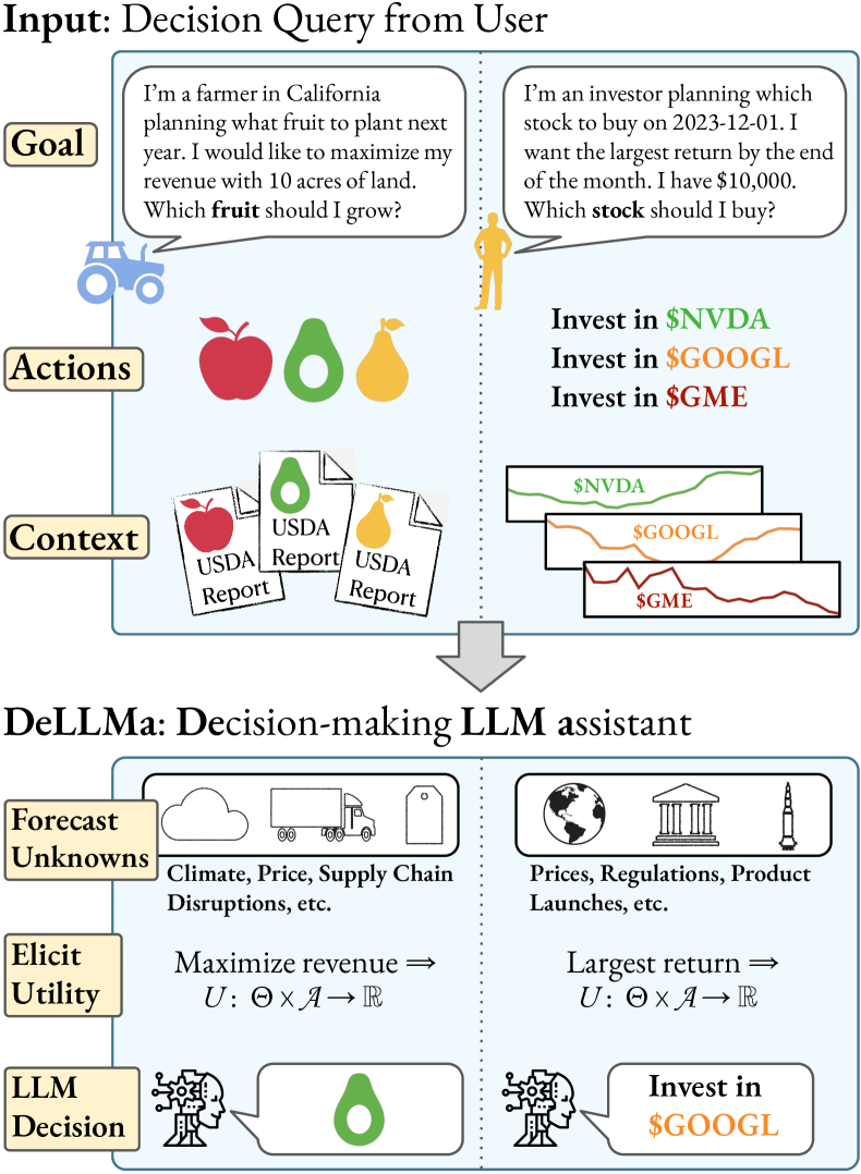
We first describe the setting in which we intend our framework to operate. Suppose a human wishes to use this LLM assistant to help make a decision. They begin by describing a decision problem via a user prompt $\mathcal{P}$. We formalize a user prompt as a triplet $\mathcal{P}=(\mathcal{G},\mathcal{A},\mathcal{C})$, which includes: a natural language description of the user’s goal $\mathcal{G}$, a list of $n$ actions $\mathcal{A}=(a_{1},\ldots,a_{n})$, and a passage of contextual information $\mathcal{C}$, which might be, e.g., pages from a report, or a text-based representation of historical data.

Referring to the Agriculture decision problem in Figure 1 as a running example, the goal $\mathcal{G}$ is for a farmer to maximize their revenue in the forthcoming year; the action set $\mathcal{A}$ lists the possible produce the farmer is interested in planting; and the context $\mathcal{C}$ consists of historical summaries of agricultural yields or information about the climate around the farm.

It is tempting to delegate such decision-making instances to LLMs with direct prompts of $\mathcal{P}$. However, we observe that responses from conventional approaches, such as Self-Consistency and CoT, do not adequately balance available evidence, handle uncertain information, or align with user preferences; we show in Section 4 that these methods perform poorly, especially with increasing numbers of actions.

[!htbp]

DeLLMa: a Decision-Making LLM Assistant.

To help encourage optimal decisions under uncertainty, we propose a framework that guides an LLM to follow the scaffolding of classical decision theory, originally designed to guide humans toward more rational decision making. By restricting LLMs to this scaffold we can also explicitly see components of the decision-making process—e.g., predictions of unknown states and utility function values—which allow a user to identify why a given decision was made.

In our initial formalization of this framework, we restrict ourselves to a slightly curtailed class of problems, and thus make a few simplifying assumptions. For example, we have assumed above that there are a discrete, enumerable set of $n$ possible actions, i.e., $\mathcal{A}=(a_{1},\ldots,a_{n})$. We will also assume there is a discrete set of $m$ possible states, $\Theta=(\theta_{1},\ldots,\theta_{m})$, though $m$ may be quite large.

Our framework will use an LLM to produce a belief distribution over the unknown states, given the input context $\mathcal{C}$. We view this as a posterior belief distribution over the states, which we denote by $\pi(\theta\mid\mathcal{C})$. Implicitly, we are assuming that the LLM implies a prior belief distribution $\pi(\theta)$, given only the model weights or training data.

Our framework will also elicit a utility function, based in part on the description of the user’s goals $\mathcal{G}\in\mathcal{P}$. This utility function will assign a real value to any state, action pair $(\theta,a)$. We denote this utility function as $U(\theta,a)$.

Given these, the expected utility under our LLM of taking an action $a$, given some additional context $\mathcal{C}$, can be written

$$U_{\mathcal{C}}(a)=\mathbb{E}_{\pi(\theta\mid\mathcal{C})}\left[U(\theta,a)\right]=\sum_{\theta\in\Theta}\pi(\theta\mid\mathcal{C})U(\theta,a).$$ (1)

Then, under the expected utility principle for rational decision making (Machina, 1987; Peterson, 2017), we should select the Bayes-optimal decision $a^{*}$, which maximizes the expected utility, and can be written

$$a^{*}=\operatorname{arg\max}_{a\in\mathcal{A}}U_{c}(a).$$ (2)

We call our framework DeLLMa, short for Decision-making Large Language Model assistant. DeLLMa carries out this sequence of four steps—state enumeration, state forecasting, utility elicitation, and expected utility maximization. A full description of DeLLMa is shown in the box below. In the following sections we give details on our specific implementation of each of these four steps.

3.1 State Enumeration

We describe the strategy that we adopt for enumerating a space of relevant latent states $\Theta=(\theta_{1},\ldots,\theta_{m})$.

Given $\mathcal{P}$ as context, we prompt an LLM to identify $k$ latent factors that are predicted to influence the user’s goal $\mathcal{G}$. Each latent factor is a string (a word or phrase), which can be viewed as describing a dimension of our state space $\Theta$. We denote these $k$ latent factors as $(f_{1},\ldots,f_{k})$.

For each latent factor, we prompt our LLM to generate $\ell$ plausible values of the latent factor (where we choose $\ell$ to be a small number such as 3). For a latent factor $f_{j}$, we denote its plausible values as $\tilde{f}_{j}^{1:\ell}$. Each of these plausible values is also a string (a word or phrase). This process discretizes the state space, where each of the $k$ dimensions has $\ell$ bins.

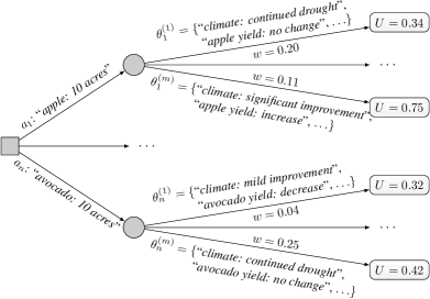
A single state $\theta_{j}$ in this state space consists of one plausible value from each of the $k$ latent factors, which we can denote by $\theta_{j}=\theta_{j}^{1:k}\in\Theta$. In total, this produces a discretized state space of size $|\Theta|=m=\ell^{k}$. While this state space is too large to enumerate explicitly, we develop a procedure to forecast probabilities for these states in a scalable manner.

3.2 State Forecasting

In the next step of DeLLMa, we must form a probabilistic forecast of the unknown states, given information contained in the provided context $\mathcal{C}\in\mathcal{P}$. We need to do this in a way that allows us to compute expected utilities, given the size of the sample space. Our strategy will be to define a joint distribution over the state space, which we can then sample from to form a Monte Carlo estimate of the expected utility.

For each of the $k$ latent factors, and each of their $\ell$ possible values $\tilde{f}_{j}^{1:\ell}$, we prompt our LLM to assign a verbalized probability score $\in$ $\{$very likely, likely, somewhat likely, somewhat unlikely, unlikely, very unlikely$\}$. In total, we must assign $k\times\ell$ of these scores. We provide concrete prompts for this verbalized probability scoring in Section C.2.

We then define a dictionary $\mathcal{V}$ that maps each verbalized probability score to a numerical value. After normalization, this scoring implies a joint probability distribution over the state space $\Theta$, assuming independence between the $k$ latent factors, which we posit for computational simplicity. We can then sample states from this joint distribution by iterating through each of the latent factors, sampling according to its approximate marginal probability (as labeled by the normalized scores), and concatenating the samples.

We describe the full procedure in Algorithm 1. As input, we provide $\mathcal{V}$, which in our implementation maps the verbalized scores to $(6,5,\cdots,1)$ in decreasing order of probability. The $\operatorname{Normalize}$ function simply scales these weights instantiated in the marginal distribution to a well-defined probability mass function (PMF). We consider the drawn samples to be from an LLM-defined proposal distribution $\pi^{\text{LLM}}(\cdot\mid\mathcal{C})$, returned as output from Algorithm 1, which approximates the posterior belief distribution $\pi(\cdot\mid\mathcal{C})$.

Algorithm 1 StateForecast$(\mathcal{M},\mathcal{P},\mathcal{V},\{f_{i},\tilde{f}_{i}^{1:\ell}\}_{i=1}^{k})$

  Input: LLM $\mathcal{M}$, user prompt $\mathcal{P}=(\mathcal{G},\mathcal{A},\mathcal{C})$, plausibilty score mapping $\mathcal{V}$, latent factors $\{f_{1},\cdots,f_{k}\}$, and plausible values $\{\tilde{f}_{1}^{1:\ell},\cdots,\tilde{f}_{k}^{1:\ell}\}$.

  for $i=1$ to $k$ do

     # PMF for the latent factor $f_{i}$

     $\pi_{i}(\cdot\mid\mathcal{C})\leftarrow\{\}$

     # Get verbalized probability scores

     $[v_{1},\cdots v_{\ell}]\leftarrow\mathcal{M}(\mathcal{P},f_{i},\tilde{f}_{i}^{1:\ell})$

     for $j=1$ to $\ell$ do

        $\pi_{j}(\tilde{f}_{i}^{j}\mid\mathcal{C})\leftarrow\mathcal{V}[v_{j}]$

     end for

     $\pi_{i}(\cdot\mid\mathcal{C})\leftarrow\operatorname{Normalize}(\pi_{i}(\cdot\mid\mathcal{C}))$

  end for

  return  $\pi^{\text{LLM}}(f_{1},\cdots,f_{k}\mid\mathcal{C})\coloneqq\prod_{i=1}^{k}\pi_{i}(\cdot\mid\mathcal{C})$

3.3 Utility Function Elicitation

Next, we need a method to elicit (which is to say: construct) a utility function $U:\Theta\times\mathcal{A}\rightarrow\mathbb{R}$, which maps a state-action pair to a real value. An accurate utility function, which balances the preferences of a human user with respect to the goal that they describe, is difficult to construct directly in a general-purpose manner. There is a long history of work on utility elicitation methods (Farquhar, 1984), which aim to construct a utility function from e.g., pairwise preference data. Here, we combine these methods with large language models to try and automatically elicit a utility function.

We conduct the following general procedure. We can sample states based on our forecast state distribution $\pi^{\text{LLM}}(\theta\mid\mathcal{C})$, and from these form a set of state-action pairs. We then group these pairs into minibatches, and prompt our LLM to rank the elements of each minibatch, given the stated user’s goal $\mathcal{G}\in\mathcal{P}$. This LLM-based ranking of items—where each item consists of an action and a particular instantation of states—is a procedure that can be broadly applied, and LLMs have a history of being successfully used for similar comparisons in prior works (Lee et al., 2024; Qin et al., 2023b). Based on these minibatch rankings, we are able to extract pairwise preferences, which we can use in classic utility elicitation algorithms.

We show this procedure in Algorithm 2 and discuss two implementations of $\operatorname{FormatRank}$: $\operatorname{Rank2Pairs}$ and $\operatorname{One-vs-All}$. Denoting $(\theta,a)_{(i)}$ as the $i$-th preferred state-action pair of the minibatch, $\operatorname{Rank2Pairs}$ converts a ranking of decreasing preference $\mathcal{R}=\left((\theta,a)_{(1)},\cdots,(\theta,a)_{(b)}\right)$ to a list of pairwise comparisons by adding $(\theta,a)_{(i)}\succ(\theta,a)_{(j)}$ whenever $i<j$. In contrast, $\operatorname{One-vs-All}$ assumes that the LLM is indifferent towards all but the top-ranked state-action pair, i.e., $\left\{(\theta,a)_{(1)}\succ(\theta,a)_{(i)}\mid\forall~{}2\leq i\leq b\right\}$. This implementation may be desirable when accurate comparisons of certain suboptimal state-actions is challenging. LLMs are also known to exhibit hallucination behavior for intensive quantitative reasoning tasks (Ji et al., 2023), and thus some middle-of-the-pack rankings may not be informative compared to the top-ranked state-action pair.

We then make use of these preferences as training data for a Bradley-Terry model (Bradley & Terry, 1952) to elicit an approximate utility function $U:\Theta\times\mathcal{A}\rightarrow\mathbb{R}$ with respect to the sampled state-action pairs.

Algorithm 2 UtilityElicitation$(\mathcal{M},\mathcal{P},\pi^{\text{LLM}},s,b,q)$

  Input: LLM $\mathcal{M}$, user prompt $\mathcal{P}=(\mathcal{G},\mathcal{A},\mathcal{C})$, proposal distribution $\pi^{\text{LLM}}(\cdot\mid\mathcal{C})$, sample size $s$, minibatch size $b$, and overlap proportion $q$.

  # Sample fixed states for each action

  $S_{A}\leftarrow\mathcal{A}\times\{\theta_{i}\mid\theta_{i}\sim\pi^{\text{LLM}}(\cdot\mid\mathcal{C}),1\leq i\leq\lfloor s/|\mathcal{A}|\rfloor\}$

  $S_{A}\leftarrow\operatorname{shuffle}(S_{A})$

  $\Omega\leftarrow\{\}$     # Pairwise comparisons

  for $i=1$ to $s$ with step $\lfloor b\times(1-q)\rfloor$ do

     # Rank the minibatch

     $\mathcal{R}\leftarrow\mathcal{M}\left(\mathcal{P},(\theta_{i},a_{i}),\cdots,(\theta_{i+b},a_{i+b})\right)$

     # Format into comparison & update

     $\Omega\leftarrow\Omega\cup\operatorname{FormatRank}(\mathcal{R})$

  end for

  return  $U(\cdot,\cdot)\coloneqq\operatorname{BradleyTerry}(\Omega)\in\mathbb{R}^{s}$

Eliciting meaningful utilities involves learning from rich preferences that ideally cover a large set of state-action samples. This desiderata presents a challenge as we observe that LLMs can behave erroneously, such as omitting or ranking candidates based on the order they appear in context. As a remedy, we discuss two ingredients that we show improve utility elicitation: batching and variance reduction.

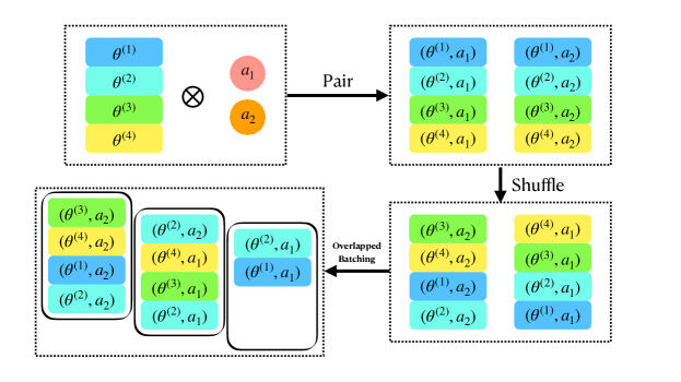
Batching

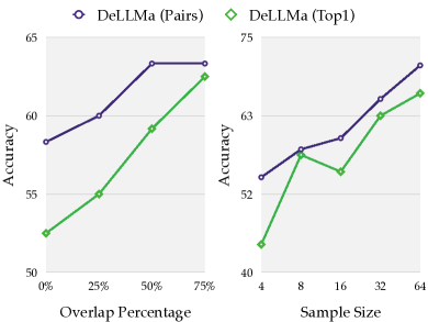
We implement a batched inference procedure that slices state-action samples $S_{A}=\{(\theta,a)\}$ into overlapping minibatches for ranking. We ensure that $q$% of samples are shared between two consecutive minibatches drawn from $S_{A}$, wherein $q$ is a hyperparameter that modulates a minibatch’s degree of exposure to the preference of the previous minibatch. Larger $q$ results in finer-grained preference at the cost of more queries. Effects of $q$ are ablated in Figure 3.

Variance Reduction

Directly sampling $|S_{A}|$ state values from the proposal distribution $\pi^{\text{LLM}}$ may lead to high-variance estimates of utilities. We instead sample $|S_{A}|/|\mathcal{A}|$ independent state values from $\pi^{\text{LLM}}$, create $|\mathcal{A}|$ duplicates, and pair them with each action $a$. See Figure 5 in Appendix A for a more intuitive illustration.

Figure 2: Results on the Agriculture environment. We show that all DeLLMa variants outperform baseline methods; DeLLMa-Pairs is the best, followed by Top1 and Naive. This result implies that the full ranking of state-action pairs is useful for utility elicitation here.

3.4 Expected Utility Maximization

As the final step in DeLLMa, we must compute the expected utility for each action, and then return the action that maximizes the expected utility.

For each action, we can compute a Monte Carlo estimate of the expected utility using state-action samples (drawn from the state forecast distribution $\pi^{\text{LLM}}(\theta\mid\mathcal{C})$), as well as the elicited utility function. Note that these calculations are all performed analytically (not via an LLM).

In particular, we can approximate the expected utility $U_{\mathcal{C}}(a)$ as a Monte Carlo estimate, written

$$U_{\mathcal{C}}(a)=\mathbb{E}_{\pi(\theta\mid\mathcal{C})}\left[U(\theta,a)\right]\approx\frac{1}{|S|}\sum_{\theta\in S}U(\theta,a),$$ (3)

given a set of state samples $S\subseteq\Theta$ drawn from our LLM-defined state forecast distribution, which is an approximation of the LLM’s posterior belief distribution about states given context $\mathcal{C}$, i.e., $S\overset{\textit{i.i.d.}}{\sim}\pi^{\text{LLM}}(\theta\mid\mathcal{C})\approx\pi(\theta\mid\mathcal{C})$.

After computing the expected utility $U_{\mathcal{C}}(a)$ for each action, DeLLMa returns the final decision to the user:

$$a^{*}=\operatorname{arg\max}_{a\in\mathcal{A}}U_{\mathcal{C}}(a).$$ (4)

4 Experiments

Figure 3: (Left) Ablation Study on sample size and overlap percentage used by DeLLMa. Increasing both parameters can produce better performance (measured by average accuracy) under both Pairs and Top1 variants. When ablating overlap percentage, we fix sample size at 16; when ablating sample size, we fix overlap percentage at 25%. (Right) Illustration of the DeLLMa decision tree for the agriculture dataset, showing two of the actions, and two of the sampled states per action. Each weight $w$ denotes the posterior probability $\pi(\theta_{i}^{(j)}\mid\mathcal{C})$.

We evaluate the performance of DeLLMa on two decision making under uncertainty problems sourced from distinct domains: agricultural planning and finance investing. Both problems involve sizable degrees of uncertainty from diverse sources, and are representative of different data modalities (natural language and tabular) involved in decision making.

We propose DeLLMa variants designed to assess algorithmic improvements outlined in Section 3.

• DeLLMa-Pairs is our de facto method that employs all techniques in §3.3 and $\operatorname{Rank2Pairs}$ for utility elicitation.

• DeLLMa-Top1 is identical to DeLLMa-Pairs, but replaces $\operatorname{Rank2Pairs}$ with $\operatorname{One-vs-All}$.

• DeLLMa-Naive represents a base version of DeLLMa-Pairs, wherein we sample different states for each action and construct pairwise comparisons from a single batch (i.e., no batching and no variance reduction).

For DeLLMa-Pairs and Top1, we allocate a per action sample size of 64 and a minibatch size of 32. We set the overlap proportion $q$ to 25% for the Agriculture dataset and 50% for the Stocks dataset due to budget constraints. For DeLLMa-Naive, we fix a total sample size of 50, which is the maximal size we observe our LLM to yield a plausible ranking without obvious hallucinations. For our LLM in all experiments shown (in all methods), we use GPT-4.

We compare DeLLMa against three baselines—zero-shot, self-consistency, and chain-of-thought, described as follows:

• Zero-Shot. Only the goal $\mathcal{G}$, the action space $\mathcal{A}$, and the context $\mathcal{C}$ is provided. We adopt a greedy decoding process by setting temperature = 0. An example prompt for each task is provided in Sections C.2 and D.

• Self-Consistency (SC) (Wang et al., 2022). We use the exact same prompt as in zero-shot, but with temperature = 0.5 to generate a divserse set of $K$ responses. We take the majority voting of the $K$ responses and record it as the final prediction. Our preliminary study finds that LLMs tend to be very confident in their decisions, and even with much higher temperature than 0.5, often all $K$ independent runs provide quite consistent decisions. We thus set $K=5$ to balance cost and performance.

• Chain-of-Thought (CoT) (Wei et al., 2022). For decision making tasks, there isn’t a standard CoT pipeline. Inspired by workflows from decision theory, we create a prompting chain consisting of three steps: (1) ask for unknown factors that impact the decision; (2) given these, ask for their possibility of occurence; (3) then ask for a final decision. Such a mechanism looks very similar to the DeLLMa pipeline (see §3) but only consists of prompting. Exampular CoT prompts are provided at Appendix D.

Evaluation Metrics.

For both datasets, our action spaces consist of a set of items, and we evaluate the performance of both DeLLMa and baseline methods by comparing the accuracy of their prediction from this set against the ground-truth optimal action (i.e., the action that maximizes ground-truth utility). We also report normalized utility—i.e., the ground-truth utility of the action chosen by a given method, normalized by the optimal ground-truth utility—in Appendix B.

We defer more involved decision-making under uncertainty problems, such as constructing a weighted combination of actions (i.e., a portfolio), to future works.

4.1 Agriculture

Data Acquisition.

We collect bi-annual reports published by the United States Department of Agriculture (USDA) that provide analysis of supply-and-demand conditions in the U.S. fruit markets. To emulate real-life farming timelines, we use the report published in September 2021 as context for planning the forthcoming agricultural year. We additionally supplement these natural language contexts with USDA-issued price and yield statistics in California.

We define the utility of planting a fruit as its price $\times$ yield reported in the forthcoming year. We identify 7 fruits—apple, avocado, grape, grapefruit, lemon, peach, and pear—that are both studied in the September 2021 report, and endowed with these statistics in 2021 and 2022. We create decision making problems by enumerating all possible combinations of availble fruits, resulting in 120 instances. For each decision-making instance, we use related sections of the USDA report and current-year price and yield statistics as context. See Section C.1 and Section C.2 for additional details on preprocesisng, and Section C.2 for DeLLMa prompts.

Figure 4: Results on the Stocks environment. We show that on average, DeLLMa-Top1 outperforms all baselines. DeLLMa-Pairs is slightly worse than its Top1 counterpart, meaning that ranking state-action pairs is still a challenging task.

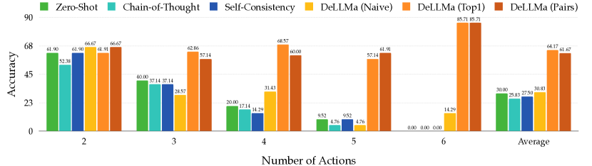
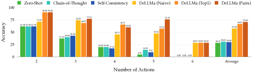
Main Result

We present our numerical results in Figure 2, and observe that all DeLLMa strategies consistently outperform baseline comparison methods, especially for larger action sets. Among DeLLMa variants, the performance of Pairs and Top1 are consistent across the board; both are significantly better than Naive. This observation demonstrates the benefits of algorithmic modifications outlined in Section 3.3; we provide more detailed analyses in the Ablation Study below.

Failure Modes of Baseline Methods

A surprising observation is that all our baseline methods consistently underperform random guessing, in the case of larger action sets. A shared failure mode is that these methods elicit decisions that echo the sentiments presented in context, and they lack the ability to reason what-if scenarios that lead to utility changes. Our experiments on SC and CoT indicate that neither sampling reasoning paths, prompting the model to imagine the alternatives, nor augmenting an LLM with a posterior belief distribution can fundamentally enhance the model’s ability to reason with uncertainty. In contrast, we ground DeLLMa methods in counterfactual scenarios via providing sampled belief states as contexts. See Section C.3 and Sections C.3, C.3 and C.3 for discussions on failure cases of baseline methods that are addressed by DeLLMa.

Ablation Study

Referring back to the Main Result, a potential explanation for the performance gap between DeLLMa-Naive and Pairs/Top1 is the discrepancy in sample size: for Naive, we allocate a fixed sample size (50) for all decision-making instances, and we allocate a fixed per action sample size (64) for Pairs and Top1. We eliminate this confounder in our ablation study, by noting that with per action sample size 8 (middle subfigure in Figure 3), DeLLMa-Pairs/Top1 achieve comparable performance to Naive, despite only receiving 16-48 samples in total for each problem instance.

In Figure 3, we observe linear performance trends when scaling up overlap percentage and sample size. Intuitively, both higher overlap percentages (i.e., more exposure between minibatches) and larger sample size lead to construction of finer-grained pairwise comparisons and thus high quality approximate utilities. Furthermore, DeLLMa-Pairs consistently outperforms Top1 for the Agriculture dataset, implicating that a nontrivial portion of the pairwise comparisons are meaningful. However, we note that the number of required API queries scales linearly with both parameters, and users are advised to choose these parameters that balance performance and cost. We report statistics for API queries and prompt lengths for our methods in Table 1 of Appendix B.

4.2 Stocks

Making decisions on stocks is a problem involving many uncertainties. Moreover, it’s fundamentally different from the agriculture decisions in many factors. Most evidently is the difference in input format – contexts for agriculture rely more on textual information (summarizations from USDA reports) whereas contexts for stocks are tabular data (historical prices per share). Stocks data are well suited to test LLMs capability in reasoning on tabular data and on highly volatile situations.

Data Acquisition.

Similar to the setup in Section 4.1, the action space $\mathcal{A}$ is limited to combinations of 7 stocks and there are in total 120 possible combinations (excluding the combinations involving single stocks). In our experiments, we choose popular stocks whose symbols are AMD, DIS, GME, GOOGL, META, NVDA and SPY. Unlike agriculture data where the context $\mathcal{C}$ are collected through USDA reports, we collect historical stock prices as the context for this problem. As illustrated in Figure 1, each stock is presented with 24 monthly price in history. In preventing possible data leakage and promoting LLMs to use their common-sense knowledge in making decisions, when using gpt4-1106-preview as the LLM checkpoint, historical price between December 2021 to November 2023 are provided as the context $\mathcal{C}$. These historical monthly prices are collected via Yahoo Finance manually by the authors.

The goal of the LLM agent is to choose which stock to invest on 2023-12-01 and sell on the last trading day of that month (2023-12-29) so that the return is maximized. Detailed prompts are presented in Appendix D. We note that we only consider the simplistic setting—choosing one stock from a set of options $\{a_{1},\cdots,a_{n}\}$.

Main Results.

Similarly, we compare three variants of DeLLMa with the three popular baselines. Shown in Figure 4, most of the observations are consistent with those in the agriculture experiments—DeLLMa’s variants outperform the baseline candidates. Unlike the agriculture setting, here DeLLMa-Naive barely improves over the baselines. We hypothesis this is due to the fact of high volatility of stocks data, that inefficient sample size without variance reduction would produce highly volatile predictors as well. This also validates the need for the design of the DeLLMa-Pairs and DeLLMa-Top1 methods.

Additionally, DeLLMa-Top1 performs better than DeLLMa-Pairs in stocks data. This is surprising at first glance since DeLLMa-Pairs have more observations in terms of pairwise preferences and ranking of sampled action-state pairs. However, upon further consideration, we hypothesize potential explanations: LLM hallucination is still an unsolved problem. For high-volatity data like stocks, LLMs can easily hallucinate with internal rankings if asked to do impossible tasks (such as to rank a batch of options where a ground-truth ranking may not exist). On the other hand, the model may still have high confidence about its prediction of the top choice in the batch. In such scenarios, using the hallucinated rankings may only provide extra noise that hinders the model performance.

5 Conclusion

We propose DeLLMa, a framework designed to harness LLMs for decision making under uncertainty in high-stakes settings. We discuss a structured approach in which we provide a scaffold for LLMs that follows the principles of classical decision theory, and then develop a feasible implementation with LLMs. Through experiments on real datasets, we highlight a systematic failure of popular prompting strategies when applied to this type of decision making task, and demonstrate the benefits of our approach to address these issues. The modularity of our framework avails many possibilities, most notably auditability and using LLMs for a broader spectrum of probablistic reasoning tasks.

Impact Statement

Rational decision making under uncertainty has been extensively studied across many disciplines, but remains elusive even for humans. Our work bears significant societal consequences as we live in a world where humans increasingly rely on intelligent assistants for diverse problems. Unfortunately, existing foundation models and LLMs are not capable of acting optimally under uncertainties yet, which may induce harm if the general public delegate these models for decision making. These risks are exacerbated when intelligent assistants operate as a black box without adequate transparency. DeLLMa serves as a first step towards an approach that builds trust for humans to rely on these systems to make important decisions under uncertainty.

Appendix A Utility Elicitation Details

In Figure 5, we show an illustration of the overlapped batching and variance reduction strategies that DeLLMa uses in its utility elicitation procedure (described in detail in Section 3.3).

Figure 5: Schematic diagram of overlapped batching and variance reduction.

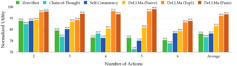
Appendix B Additional Results

In Figures 6 and 7 we show the normalized utility (i.e., ground-truth utility of the chosen action, normalized by the maximum ground-truth utility) of each method. These results can be contrasted against the accuracy of each method’s prediction of the optimal action in Figures 2 and 4.

Figure 6: Normalized utility for the Agriculture dataset. Across all action sizes, DeLLMa-Pairs/Top1 outperforms other methods, including DeLLMa-Naive. Similar to accuracy, DeLLMa-Pairs slightly outperforms Top1, which is consistent with our hypothesis that the complete ranking generated from GPT-4 is meaningful.

Figure 7: Normalized utility for the Stock dataset. DeLLMa-Top1 is competitive againt Pairs, suggesting that financial decision making may be a challenging scenario for GPT-4 to elicit preference unequivocally.

Aside from performance improvements, we also compare the cost measured in terms of prompt length and API calls in Table 1. For the Agriculture dataset, DeLLMa-Naive is comparable to SC in terms of prompt length and significantly outperform the latter, while only requiring 20% of API calls. DeLLMa-Pairs/Top1 can push the performance further, but incurs a higher cost, especially for large sample sizes.

	Zero-Shot	CoT	SC	DeLLMa-Naive	DeLLMa-Pairs (16)	DeLLMa-Pairs (64)
API Calls	1	3	5	1	3	10
Word Counts	693.71	2724.2	3468.55	3681.94	7254.46	28895.46

Table 1: Number of GPT-4 API calls and word counts per decision-making instance (with action set size 4 for the Agriculture dataset) across all methods discussed in Section 4. For DeLLMa-Naive, we set the total sample size to 50. For DeLLMa-Pairs, we fix the overlap percentage to 25% and vary the per action sample size from 16 to 64. DeLLMa-Top1 has the same statistics as DeLLMa-Pairs since they only differ in post processing.

Appendix C Additional Details for Agriculture

C.1 Dataset Curation

To reduce context length, we make use of GPT-4 to provide executive and per-fruit summaries of the report, reducing the context length from 8,721 words ($\sim$12,000 tokens) to $<700$ words ($\sim$1,000 tokens). We proof-read these summaries to ensure that they do not contain any factual errors. For each decision-making instance, we use the executive summary, the summaries relevant to the fruits in consideration, and their current-year price and yield statistics as context. We provide prompt for summarizing the report in Section C.2, and report concrete summaries and statistics in supplementary materials.

C.2 Prompt Used by Agriculture

We first present in Section C.2 the prompt used for summarizing the context in our Agriculture experiments. These summaries are used for all methods including baselines and DeLLMa variants.

[!htbp]

We now present in Section C.2 the prompt for Zero-Shot experiments consisting of $\mathcal{P}=(\mathcal{G},\mathcal{C},\mathcal{A})$, with summaries generated from Section C.2 as context. All other baselines and DeLLMa agents extend from this prompt.

[!htbp]

Section C.2 illustrates an exemplar prompt for DeLLMa agent on the Agriculture dataset. All DeLLMa variants follow the same prompt structure, but differs in the means state-action pairs are prepared.

[!htbp]

In Section C.2 we present the prompt for state enumeration and state forecasting for the Agriculture dataset. Our implementation combines these two modules, but in the future they should be separate as our framework continues to progress. For example, state enumeration may leverage retrieval-augmented generation (Lewis et al., 2020) for generating high-quality unknown factors, and state forecasting may resort to tool usage to delibrate calibrated belief distributions from quanitative analysis.

[!htbp]

C.3 Failure Cases on the Agriculture Dataset

In Section 4, we postulate that a failure mode of our baseline approaches is that they lack the ability to perform probablistic reasoning, but are rather following the sentiment presented in context. Here, we qualitatively test this hypothesis, by showcasing prompts and responses from our Zero-Shot experiments. We present instances in Sections C.3, C.3 and C.3 that are not able to make optimal prediction with baseline methods, but are solved by DeLLMa agents.

Within each figure, we first present $\mathcal{P}$, followed by the (incorrect) decision and explanation generated from the Zero-Shot baseline, and then present the top-ranked state action pair generated by DeLLMa along with its explanation.

[!htbp]

In the case of deciding between apple and grapefruit in Section C.3, GPT-4 presumes that a high price for grapefruit is sustainable due to the presence of extreme weather conditions in the previous year. With CoT, the model reasons with some counterfactual scenarios, such as more suitable weather for the forthcoming year, but not in a systematic way. With DeLLMa, we provide these a list of counterfactual scenarios as context, and leverage the model’s ability for situational thinking and ranking to elicit an informative preference. We make similar observations for Sections C.3 and C.3

[!htbp]

[!htbp]

Appendix D Prompts Used by Stocks

Similar to the agriculture setup, we first present a sample zero-shot prompt in Appendix D.

[!htbp]

The zero-shot prompt consists of three main parts (see Figure 1 for visual illustrations): (1) an enumeration of action spaces (here AMD or GME), (2) a provided context (here, historical stock prices between December 2021 to November 2023), and (3) the goal of the user (choose only one stock to maximize their profit via investing in stocks).

Similarly, we examplify a prompt for Chain-of-Thought. Notably, we break the chain into three parts in Appendix D: (1) Enumerating unknown factors, (2) Enumerating $\pi^{\text{LLM}}(\cdot\mid\mathcal{C})$, and (3) making the final decision given the previous responses and context.

[!htbp]

Finally, we showcase the DeLLMa ranking prompts where the LLM is asked to provide comprehensive rankings of given state-action pairs.

[!htbp]

References

- Bazerman & Moore (2012) Bazerman, M. H. and Moore, D. A. Judgment in managerial decision making. John Wiley & Sons, 2012.
- Benary et al. (2023) Benary, M., Wang, X. D., Schmidt, M., Soll, D., Hilfenhaus, G., Nassir, M., Sigler, C., Knödler, M., Keller, U., Beule, D., et al. Leveraging large language models for decision support in personalized oncology. JAMA Network Open, 6(11):e2343689–e2343689, 2023.
- Berger (2013) Berger, J. O. Statistical decision theory and Bayesian analysis. Springer Science & Business Media, 2013.
- Bommasani et al. (2021) Bommasani, R., Hudson, D. A., Adeli, E., Altman, R., Arora, S., von Arx, S., Bernstein, M. S., Bohg, J., Bosselut, A., Brunskill, E., et al. On the opportunities and risks of foundation models. arXiv preprint arXiv:2108.07258, 2021.
- Bradley & Terry (1952) Bradley, R. A. and Terry, M. E. Rank analysis of incomplete block designs: I. the method of paired comparisons. Biometrika, 39(3/4):324–345, 1952.
- Bubeck et al. (2023) Bubeck, S., Chandrasekaran, V., Eldan, R., Gehrke, J., Horvitz, E., Kamar, E., Lee, P., Lee, Y. T., Li, Y., Lundberg, S., et al. Sparks of artificial general intelligence: Early experiments with gpt-4. arXiv preprint arXiv:2303.12712, 2023.
- Chen & Mueller (2023) Chen, J. and Mueller, J. W. Quantifying uncertainty in answers from any language model via intrinsic and extrinsic confidence assessment. ArXiv, abs/2308.16175, 2023. URL https://api.semanticscholar.org/CorpusID:261339369.
- Farquhar (1984) Farquhar, P. H. State of the art—utility assessment methods. Management science, 30(11):1283–1300, 1984.
- Ferrara (2023) Ferrara, E. Should chatgpt be biased? challenges and risks of bias in large language models. arXiv preprint arXiv:2304.03738, 2023.
- Fishburn (1968) Fishburn, P. C. Utility theory. Management science, 14(5):335–378, 1968.
- Hao et al. (2023) Hao, S., Gu, Y., Ma, H., Hong, J. J., Wang, Z., Wang, D. Z., and Hu, Z. Reasoning with language model is planning with world model. arXiv preprint arXiv:2305.14992, 2023.
- Ji et al. (2023) Ji, Z., Lee, N., Frieske, R., Yu, T., Su, D., Xu, Y., Ishii, E., Bang, Y. J., Madotto, A., and Fung, P. Survey of hallucination in natural language generation. ACM Computing Surveys, 55(12):1–38, 2023.
- Kadavath et al. (2022) Kadavath, S., Conerly, T., Askell, A., Henighan, T., Drain, D., Perez, E., Schiefer, N., Hatfield-Dodds, Z., DasSarma, N., Tran-Johnson, E., Johnston, S., El-Showk, S., Jones, A., Elhage, N., Hume, T., Chen, A., Bai, Y., Bowman, S., Fort, S., Ganguli, D., Hernandez, D., Jacobson, J., Kernion, J., Kravec, S., Lovitt, L., Ndousse, K., Olsson, C., Ringer, S., Amodei, D., Brown, T., Clark, J., Joseph, N., Mann, B., McCandlish, S., Olah, C., and Kaplan, J. Language models (mostly) know what they know, 2022.
- Kochenderfer (2015) Kochenderfer, M. J. Decision making under uncertainty: theory and application. MIT press, 2015.
- Kochenderfer et al. (2022) Kochenderfer, M. J., Wheeler, T. A., and Wray, K. H. Algorithms for decision making. MIT press, 2022.
- Lee et al. (2024) Lee, H., Phatale, S., Mansoor, H., Mesnard, T., Ferret, J., Lu, K., Bishop, C., Hall, E., Carbune, V., Rastogi, A., and Prakash, S. RLAIF: Scaling reinforcement learning from human feedback with ai feedback, 2024. URL https://openreview.net/forum?id=AAxIs3D2ZZ.
- Lewis et al. (2020) Lewis, P., Perez, E., Piktus, A., Petroni, F., Karpukhin, V., Goyal, N., Küttler, H., Lewis, M., Yih, W.-t., Rocktäschel, T., et al. Retrieval-augmented generation for knowledge-intensive nlp tasks. Advances in Neural Information Processing Systems, 33:9459–9474, 2020.
- Li et al. (2023) Li, B., Mellou, K., Zhang, B., Pathuri, J., and Menache, I. Large language models for supply chain optimization, 2023.
- Lin et al. (2022) Lin, S., Hilton, J., and Evans, O. Teaching models to express their uncertainty in words, 2022.
- Lin et al. (2023) Lin, Z., Trivedi, S., and Sun, J. Generating with confidence: Uncertainty quantification for black-box large language models, 2023.
- Luce & Raiffa (1989) Luce, R. D. and Raiffa, H. Games and decisions: Introduction and critical survey. Courier Corporation, 1989.
- Machina (1987) Machina, M. J. Choice under uncertainty: Problems solved and unsolved. Journal of Economic Perspectives, 1(1):121–154, 1987.
- Mao et al. (2023) Mao, J., Ye, J., Qian, Y., Pavone, M., and Wang, Y. A language agent for autonomous driving, 2023.
- Mielke et al. (2022) Mielke, S. J., Szlam, A., Dinan, E., and Boureau, Y.-L. Reducing conversational agents’ overconfidence through linguistic calibration, 2022.
- Nie et al. (2023) Nie, A., Cheng, C.-A., Kolobov, A., and Swaminathan, A. Importance of directional feedback for llm-based optimizers. In NeurIPS 2023 Foundation Models for Decision Making Workshop, 2023.
- Peterson (2017) Peterson, M. An introduction to decision theory. Cambridge University Press, 2017.
- Qin et al. (2023a) Qin, Y., Liang, S., Ye, Y., Zhu, K., Yan, L., Lu, Y., Lin, Y., Cong, X., Tang, X., Qian, B., et al. Toolllm: Facilitating large language models to master 16000+ real-world apis. arXiv preprint arXiv:2307.16789, 2023a.
- Qin et al. (2023b) Qin, Z., Jagerman, R., Hui, K., Zhuang, H., Wu, J., Shen, J., Liu, T., Liu, J., Metzler, D., Wang, X., and Bendersky, M. Large language models are effective text rankers with pairwise ranking prompting, 2023b.
- Ren et al. (2023) Ren, A. Z., Dixit, A., Bodrova, A., Singh, S., Tu, S., Brown, N., Xu, P., Takayama, L., Xia, F., Varley, J., Xu, Z., Sadigh, D., Zeng, A., and Majumdar, A. Robots that ask for help: Uncertainty alignment for large language model planners. ArXiv, abs/2307.01928, 2023. URL https://api.semanticscholar.org/CorpusID:259342058.
- Schoemaker (1982) Schoemaker, P. J. The expected utility model: Its variants, purposes, evidence and limitations. Journal of economic literature, pp. 529–563, 1982.
- Shinn et al. (2023) Shinn, N., Cassano, F., Gopinath, A., Narasimhan, K. R., and Yao, S. Reflexion: Language agents with verbal reinforcement learning. In Thirty-seventh Conference on Neural Information Processing Systems, 2023.
- Si et al. (2022) Si, C., Zhao, C., Min, S., and Boyd-Graber, J. Re-examining calibration: The case of question answering. In Goldberg, Y., Kozareva, Z., and Zhang, Y. (eds.), Findings of the Association for Computational Linguistics: EMNLP 2022, pp. 2814–2829, Abu Dhabi, United Arab Emirates, December 2022. Association for Computational Linguistics. doi: 10.18653/v1/2022.findings-emnlp.204. URL https://aclanthology.org/2022.findings-emnlp.204.
- Thirunavukarasu et al. (2023) Thirunavukarasu, A. J., Ting, D. S. J., Elangovan, K., Gutierrez, L., Tan, T. F., and Ting, D. S. W. Large language models in medicine. Nature medicine, 29(8):1930–1940, 2023.
- Von Neumann & Morgenstern (1944) Von Neumann, J. and Morgenstern, O. Theory of games and economic behavior. 1944.
- Wang et al. (2022) Wang, X., Wei, J., Schuurmans, D., Le, Q. V., Chi, E. H., Narang, S., Chowdhery, A., and Zhou, D. Self-consistency improves chain of thought reasoning in language models. In The Eleventh International Conference on Learning Representations, 2022.
- Wei et al. (2022) Wei, J., Wang, X., Schuurmans, D., Bosma, M., Xia, F., Chi, E., Le, Q. V., Zhou, D., et al. Chain-of-thought prompting elicits reasoning in large language models. Advances in Neural Information Processing Systems, 35:24824–24837, 2022.
- Yang et al. (2023) Yang, C., Wang, X., Lu, Y., Liu, H., Le, Q. V., Zhou, D., and Chen, X. Large language models as optimizers. arXiv preprint arXiv:2309.03409, 2023.
- Yao et al. (2023) Yao, S., Yu, D., Zhao, J., Shafran, I., Griffiths, T. L., Cao, Y., and Narasimhan, K. Tree of thoughts: Deliberate problem solving with large language models. arXiv preprint arXiv:2305.10601, 2023.
- Ye et al. (2023) Ye, Y., Cong, X., Qin, Y., Lin, Y., Liu, Z., and Sun, M. Large language model as autonomous decision maker. arXiv preprint arXiv:2308.12519, 2023.
- Zhuang et al. (2023) Zhuang, Y., Chen, X., Yu, T., Mitra, S., Bursztyn, V., Rossi, R. A., Sarkhel, S., and Zhang, C. Toolchain*: Efficient action space navigation in large language models with a* search. arXiv preprint arXiv:2310.13227, 2023.