Variational Quantum AdaBoost with Supervised Learning Guarantee

Abstract

Although variational quantum algorithms based on parameterized quantum circuits promise to achieve quantum advantages, in the noisy intermediate-scale quantum (NISQ) era, their capabilities are greatly constrained due to limited number of qubits and depth of quantum circuits. Therefore, we may view these variational quantum algorithms as weak learners in supervised learning. Ensemble methods are a general technique in machine learning for combining weak learners to construct a more accurate one. In this paper, we theoretically prove and numerically verify a learning guarantee for variational quantum adaptive boosting (AdaBoost). To be specific, we theoretically depict how the prediction error of variational quantum AdaBoost on binary classification decreases with the increase of the number of boosting rounds and sample size. By employing quantum convolutional neural networks, we further demonstrate that variational quantum AdaBoost can not only achieve much higher accuracy in prediction, but also help mitigate the impact of noise. Our work indicates that in the current NISQ era, introducing appropriate ensemble methods is particularly valuable in improving the performance of quantum machine learning algorithms.

I Introduction

I.1 Background

Machine learning has achieved remarkable success in various fields with a wide range of applications [1, 2, 3, 4]. A major objective of machine learning is to develop efficient and accurate prediction algorithms, even for large-scale problems [5, 6]. The figure of merit, prediction error, can be decomposed into the summation of training and generalization errors. Both of them should be made small to guarantee an accurate prediction. However, there is a tradeoff between reducing the training error and restricting the generalization error through controlling the size of the hypothesis set, known as Occam’s Razor principle [7].

For classical machine learning, empirical studies have demonstrated that the training error can often be effectively minimized despite the non-convex nature and abundance of spurious minima in training loss landscapes [8, 9]. This observation has been explained by the theory of over-parameterization [10, 11, 12, 13]. However, it is still difficult to theoretically describe how to guarantee a good generalization, which is one of the key problems to be solved in classical machine learning.

Owing to the immense potential of quantum computing, extensive efforts have been dedicated to developing quantum machine learning [14, 15, 16, 17, 18]. However, in the noisy intermediate-scale quantum (NISQ) era, the capability of quantum machine learning is greatly constrained due to limited number of qubits and depth of the involved quantum circuits. Algorithms based on parameterized quantum circuits (PQCs) have become the leading candidates to yield potential quantum advantages in the era of NISQ [19]. The basic idea behind them is that these parameterized quantum models can provide representational and/or computational powers beyond what is possible with classical models [20, 21, 22, 23]. There are mainly three kinds of parameterized quantum models [24]: (a) explicit models [25, 26], where data are first encoded into quantum states, after undergoing a PQC, the quantum states are measured and the information is used to update the variational parameters through a classical routine; (b) implicit kernel models [27, 28], where the kernel matrices of the encoding data are computed through quantum circuits, and then used to label data; (c) re-uploading models [29], where encoding and parameterized circuits are interleaved. A unified framework has been set in [24] for the three quantum models, and it was pointed out that the advantages of quantum machine learning may lie beyond kernel methods. They found that although kernel methods are guaranteed to achieve a lower training error, their generalization power is poor. Thus, both the training and generalization errors should be taken into account when evaluating the prediction accuracy [30].

It has been proved in [31] that good generalization can be guaranteed from few training data for a wide range of quantum machine learning models. However, in contrast to the classical case, training quantum models is notoriously difficult as it often suffers from the phenomena of barren plateaus [32, 33, 34, 35, 36, 37, 38], where the cost gradient vanishes exponentially fast, and there exist (exponentially) many spurious local minima [39, 40]. In this sense, most quantum learning algorithms can be viewed as weak learners in the language of supervised machine learning.

To improve the performance of quantum algorithms, we can employ ensemble methods as inspired by the classical ensemble learning. There are various kinds of ensemble methods, e.g., bagging [41], plurality voting [42, 43] and boosting [44]. It has been suggested in [45] that an optimized weighted mixture of concepts, e.g., PAC-Bayesian [46], is a promising candidate for further research. Thus, adaptive boosting (AdaBoost), which adaptively adjusts the weights of a set of base learners to construct a more accurate learner than base learners, is appropriate for improving the performance of quantum weak learners. For classical machine learning, there has been a rich theoretical analysis on AdaBoost [47, 48, 49], and it has been shown to be effective in practice [50, 51, 52, 53]. In this paper, we provide the first theoretical learning guarantee for binary classification of variational quantum AdaBoost, and then numerically investigate its performance on 4-class classification by employing quantum convolutional neural networks (QCNNs), which are naturally shallow and particularly useful in NISQ era.

I.2 Related Work

Various quantum versions of classical AdaBoost have been proposed, such as  [54, 55, 56]. In their works, they employed quantum subroutines, e.g., mean estimation and amplitude amplification, to update quantum weak classifiers and estimate the weighted errors to reduce the time complexity. Therefore, the realizations of these quantum versions of AdaBoost are beyond the scope of current NISQ circuits. In contrast, in this paper, we utilize variational quantum classifiers realized on current NISQ circuits, which are implemented through a quantum-classical hybrid way.

Recently, ensemble methods have been proposed to enhance the accuracy and robustness of quantum classification with NISQ devices. Variational quantum AdaBoost and variational quantum Bagging have been empirically investigated in [57, 58] with hardware-efficient ansatz. It was empirically demonstrated that quantum AdaBoost not only outperforms quantum Bagging [57], but also can save resources in terms of the number of qubits, gates, and training samples [58].

I.3 Our Contributions

In this paper, we theoretically and numerically investigate the performance of variational quantum AdaBoost by focusing on classification. Our contributions are summarized as follows.

1. For binary classification, we provide the first theoretical upper bound on the prediction error of variational quantum AdaBoost, demonstrating how the prediction error converges to 0 as the increase of the number of boosting rounds and sample size.

2. We numerically demonstrate that variational quantum AdaBoost can achieve a higher level of prediction accuracy as compared to quantum Bagging, classical AdaBoost and classical Bagging. We further demonstrate that with only few boosting rounds variational quantum AdaBoost can help mitigate the impact of noises and achieve better performance than noiseless models, which is particularly valuable for potential applications, especially in the NISQ era.

The paper is organized as follows. In Section II, we briefly introduce the quantum classifier and variational quantum AdaBoost. In Section III, we present our theoretical and empirical results on the performance of variational quantum AdaBoost. Section IV concludes the paper.

II Quantum classifier and AdaBoost

II.1 Quantum Classifier

We start with briefly introducing some quantum notation. In quantum computing, information is described in terms of quantum states. For an $N$-qubit system, the quantum state $\rho$ can be mathematically represented as a positive semi-definite Hermitian matrix $\rho\in\mathbb{C}^{2^{N}\times 2^{N}}$ with $\mathrm{Tr}\left[\rho\right]=1$. The elementary quantum gates are mathematically described by unitary matrices. A quantum gate $U$ acting on a quantum state $\rho$ takes the state to the output state as $U\rho U^{{\dagger}}$ where $U^{{\dagger}}$ is the conjugate and transpose of $U$. When measuring an observable $O$, which is a Hermitian operator, at quantum state $\rho$, its expectation is ${\rm Tr}\left[O\rho\right]$.

For a $D$-class classification problem, suppose that both the training and test data are independent and identically distributed (i.i.d.) according to some fixed but unknown distribution $\mathcal{D}$ defined over the sample and label space $\mathcal{X}\times\mathcal{Y}$. When the sample set $S=\left\{\left(\bm{x}_{i},y_{i}\right)\right\}_{i=1}^{n}$ are classical, we can first choose a quantum encoding circuit to embed the classical data $\bm{x}_{i}$ into quantum state $\rho\left(\bm{x}_{i}\right)$ [20, 59, 60]. We thus focus on the explicit quantum model [24]. Without loss of generality, we only consider the case where the data are quantum in the following, namely, $S={\left\{\left(\rho\left(\bm{x}_{i}\right),y_{i}\right)\right\}}^{n}_{i=1}\subset\mathcal{X}\times\mathcal{Y}$. For a $D$-class classification, $\mathcal{Y}=\left\{1,\cdots,D\right\}\triangleq\left[D\right]$.

To label $\rho(\bm{x})$, a quantum hypothesis or classifier $h_{\bm{\theta}}(\cdot)$ can be described in the form of

$$h_{\bm{\theta}}\left(\bm{x}\right)=\mathop{\arg\max}\limits_{d\in\left[D\right]}{\rm Tr}\left[P_{d}U\left(\bm{\theta}\right)\rho\left(\bm{x}\right)U^{\dagger}\left(\bm{\theta}\right)\right].$$ (1)

Here, $\left\{P_{d}\right\}^{D}_{d=1}$ are disjoint projectors with $P_{d}$ relating to the $d$-th class for $d\in\left[D\right]$, and $U\left(\bm{\theta}\right)$ describes the action of a PQC with $\bm{\theta}$ being the trainable or variational parameters.

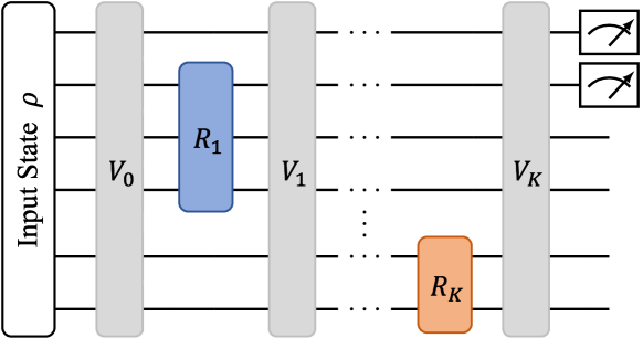
Figure 1: The schematic of a PQC with $K$ independent trainable gates. Each trainable gate is parameterized by a multi-qubit rotational gate which is efficiently implementable.

To be specific, as illustrated in Fig. 1, suppose that the employed PQC is composed of a total number of $K$ independent parameterized gates and non-trainable gates $\{V_{k}\}^{K}_{k=0}$, whose action can be described as

$$U\left(\bm{\theta}\right)=\prod^{K}_{k=1}\Big{[}V_{k}{R_{k}^{\left(i_{k},j_{k}\right)}\left(\theta_{k}\right)}\Big{]}\cdot V_{0},$$ (2)

where $\bm{\theta}=\left(\theta_{1},\cdots,\theta_{K}\right)$ denotes a $K$-dimensional parameter vector. For each $k$, the trainable gate $R_{k}^{\left(i_{k},j_{k}\right)}\left(\theta_{k}\right)$ denotes a rotational gate with angle $\theta_{k}$ around a $j_{k}$-qubit Pauli tensor product operator $P_{k}$, which acts non-trivially on the $i_{k}$-th through to $\left(i_{k}+j_{k}-1\right)$-th qubits, namely,

$$R_{k}^{\left(i_{k},j_{k}\right)}\left(\theta_{k}\right)=I^{\otimes\left(i_{k}-1\right)}\otimes e^{-i\frac{\theta_{k}}{2}P_{k}}\otimes I^{\otimes\left(n-i_{k}-j_{k}+1\right)}$$

$$= I^{\otimes\left(i_{k}-1\right)}\otimes\left(\cos\frac{\theta_{k}}{2}I^{\otimes j_{k}}-i\sin\frac{\theta_{k}}{2}P_{k}\right)\otimes I^{\otimes\left(n-i_{k}-j_{k}+1\right)}.$$

In practice, these multi-qubit rotational gates can be implemented by a series of single-qubit gates and typical $2$-qubit controlled gates, which are efficient to realize. For example, as illustrated in Fig. 2, the multi-qubit rotational gates around $z$ axis can be implemented by a single-qubit rotational gate around $z$ axis and some $2$-qubit CNOT gates.

The prediction error or expected risk of the quantum hypothesis function $h_{\bm{\theta}}$ is defined as

$$R\left(h_{\bm{\theta}}\right)=\mathop{\mathbb{E}}\limits_{\left(\bm{x},y\right)\sim\mathcal{D}}{\mathbb{I}_{h_{\bm{\theta}}\left(\bm{x}\right)\neq y}}=\mathop{\mathbb{P}}\limits_{\left(\bm{x},y\right)\sim\mathcal{D}}{\left[\,h_{\bm{\theta}}\left(\bm{x}\right)\neq y\,\right]}.$$ (3)

The prediction error of a hypothesis is not directly accessible, since both the label of unseen data and the distribution $\mathcal{D}$ are unavailable. However, we can take the training error or empirical risk of $h_{\bm{\theta}}$ as a proxy, defined as

$$\widehat{R}_{S}\left(h_{\bm{\theta}}\right)=\frac{1}{n}\sum_{i=1}^{n}{\mathbb{I}_{h_{\bm{\theta}}\left(\bm{x}_{i}\right)\neq y_{i}}}.$$ (4)

The difference between the prediction error $R\left(h_{\bm{\theta}}\right)$ and the training error $\widehat{R}_{S}\left(h_{\bm{\theta}}\right)$ is referred to as the generalization error, which reads

$$\texttt{gen}\left(h_{\bm{\theta}}\right)=R\left(h_{\bm{\theta}}\right)-\widehat{R}_{S}\left(h_{\bm{\theta}}\right).$$ (5)

It is clear that to make accurate predictions, both the training and generalization errors should be small.

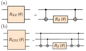
Figure 2: Hardware-efficient implementations of multi-qubit rotational gates. (a) The module of $2$-qubit rotational gate $R_{ZZ}\left(\theta\right)$ around the Pauli operator $Z\otimes Z$. (b) The module of $3$-qubit rotational gate $R_{ZZZ}\left(\theta\right)$ around the Pauli operator $Z\otimes Z\otimes Z$.

II.2 Variational Quantum AdaBoost

We denote by $\mathcal{H}$ the hypothesis set which is composed of base classifiers $h_{\bm{\theta}}\left(\cdot\right)$ in the form of Eq. (1). Inspired by classical multi-class AdaBoost [61], the procedure of variational quantum AdaBoost is presented in Algorithm 1, which is similar to that in [57].

input : Hypothesis set $\mathcal{H}=\left\{h_{\bm{\theta}}\right\}$

Sample set $S={\left\{\left(\rho\left(\bm{x}_{i}\right),y_{i}\right)\right\}}^{n}_{i=1}$

Boosting rounds $T$

Distribution $\mathcal{D}_{1}\left(i\right)=\frac{1}{n}$, for $i\in\left[n\right]$

for $t\leftarrow 1$ to $T$ do

       $h_{t}\leftarrow$ base classifier in $\mathcal{H}$ with error $\epsilon_{t}<\frac{D-1}{D}$ $\alpha_{t}\leftarrow\log{\frac{1-\epsilon_{t}}{\epsilon_{t}}}+\log{\left(D-1\right)}$ for $i\leftarrow 1$ to $n$ do

             $\mathcal{D}_{t+1}\left(i\right)\leftarrow\mathcal{D}_{t}\left(i\right)\exp{\left[\alpha_{t}\mathbb{I}_{y_{i}\neq h_{t}\left(\bm{x}_{i}\right)}\right]}$

       end for

      normalize $\left\{\mathcal{D}_{t+1}\left(i\right)\right\}_{i=1}^{n}$

end for

$f\leftarrow\mathop{\arg\max}\limits_{d\in\left[D\right]}{\sum_{t=1}^{T}{\alpha_{t}\mathbb{I}_{h_{t}=d}}}$ output : Predictor $f$

Algorithm 1 $D$-Class Variational Quantum AdaBoost

Algorithm 1 has the input including a labeled sample set $S={\left\{\left(\rho\left(\bm{x}_{i}\right),y_{i}\right)\right\}}^{n}_{i=1}$, the number of boosting rounds $T$ typically selected via cross-validation, and maintains a distribution over the indices $\left[n\right]$ for each round. The initial distribution is assumed to be uniform, i.e., $\mathcal{D}_{1}\left(i\right)=\frac{1}{n}$. At each round of boosting, i.e., for each $t\in\left[T\right]$, given a classifier $h_{t}\in\mathcal{H}$, its error $\epsilon_{t}$ on the training data weighted by the distribution $\mathcal{D}_{t}$ reads

$$\epsilon_{t}=\sum_{i=1}^{n}{\mathcal{D}_{t}\left(i\right)\mathbb{I}_{h_{t}\left(\bm{x}_{i}\right)\neq y_{i}}}.$$ (6)

We choose a weak classifier $h_{t}$ such that $\epsilon_{t}<\frac{D-1}{D}$, which is easily satisfied. Then the distribution is updated as $\mathcal{D}_{t+1}\left(i\right)\propto\mathcal{D}_{t}\left(i\right)\exp{\left[\alpha_{t}\mathbb{I}_{y_{i}\neq h_{t}\left(\bm{x}_{i}\right)}\right]}$, where $\alpha_{t}=\log\frac{1-\epsilon_{t}}{\epsilon_{t}}+\log\left(D-1\right)$. After $T$ rounds of boosting, Algorithm 1 returns the $D$-class quantum AdaBoost classifier.

III Main Results

III.1 Binary Variational Quantum AdaBoost Guarantee

For multi-class classification, an alternative approach is to reduce the problem to that of multiple binary classification tasks. For each task, a binary classifier is returned, and the multi-class classifier is defined by a combination of these binary classifiers. Two standard reduction techniques are one-versus-the-rest and one-versus-one [5]. In this subsection, we focus on the basic binary variaitonal quantum AdaBoost, and theoretically establish its learning guarantee.

For binary classification, it is more convenient to denote the label space by $\mathcal{Y}=\left\{-1,+1\right\}$. The base quantum hypothesis $h_{\bm{\theta}}\left(\cdot\right)$ can be defined in terms of the Pauli-$Z$ operator $Z=\begin{pmatrix}1&0\\ 0&-1\end{pmatrix}$ as

$$h_{\bm{\theta}}\left(\bm{x}\right)={\rm Tr}\left[ZU\left(\bm{\theta}\right)\rho\left(\bm{x}\right)U^{\dagger}\left(\bm{\theta}\right)\right],$$ (7)

whose range is $\left[-1,+1\right]$, and its sign is used to determine the label, namely, we label $-1$ when $h_{\bm{\theta}}\left(\bm{x}\right)\leq 0$; otherwise, it is labeled as $+1$.

It is straightforward to verify that for a sample $\left(\rho\left(\bm{x}\right),y\right)$, the following important relation holds:

$$\mathbb{I}_{y\neq h_{\bm{\theta}}\left(\bm{x}\right)}=\mathbb{I}_{yh_{\bm{\theta}}\left(\bm{x}\right)\leq 0}.$$ (8)

By employing Eq. (8) and inspired by the classical binary AdaBoost [5], we can modify Algorithm 1 slightly to make it more suitable for binary classification as presented in Algorithm 2, and further establish the learning guarantee for the binary variational quantum AdaBoost.

Different from Algorithm 1, the hypothesis set $\mathcal{H}$ in Algorithm 2 is composed of quantum hypothesis in the form of Eq. (7). At each round of boosting, a new classifier $h_{t}\in\mathcal{H}$ is selected such that its error $\epsilon_{t}<\frac{1}{2}$, and the distribution update role

$$\mathcal{D}_{t+1}\left(i\right)=\frac{\mathcal{D}_{t}\left(i\right)\exp{\left(-\alpha_{t}y_{i}h_{t}\left(x_{i}\right)\right)}}{Z_{t}}$$

is different from what is used in Algorithm 1. It can be verified that $\alpha_{t}=\frac{1}{2}\log\frac{1-\epsilon_{t}}{\epsilon_{t}}$ is chosen to minimize the upper bound of the empirical risk $\widehat{R}_{S}\left(f\right)$ of the binary variational quantum AdaBoost [5].

input : Hypothesis set $\mathcal{H}=\left\{h_{\bm{\theta}}\right\}$

Sample set $S={\left\{\left(\rho\left(\bm{x}_{i}\right),y_{i}\right)\right\}}^{n}_{i=1}$

Boosting rounds $T$

Distribution $\mathcal{D}_{1}\left(i\right)=\frac{1}{n}$, for $i\in\left[n\right]$

for $t\leftarrow 1$ to $T$ do

       $h_{t}\leftarrow$ base classifier in $\mathcal{H}$ with error $\epsilon_{t}<\frac{1}{2}$ $\alpha_{t}\leftarrow\frac{1}{2}\log{\frac{1-\epsilon_{t}}{\epsilon_{t}}}$ $Z_{t}\leftarrow 2{\left[\epsilon_{t}\left(1-\epsilon_{t}\right)\right]}^{\frac{1}{2}}\$    //normalization factor for $i\leftarrow 1$ to $n$ do

             $\mathcal{D}_{t+1}\left(i\right)\leftarrow\frac{\mathcal{D}_{t}\left(i\right)\exp{\left[-\alpha_{t}y_{i}h_{t}\left(x_{i}\right)\right]}}{Z_{t}}$

       end for

      

end for

$f\leftarrow\text{sgn}{\left(\sum_{t=1}^{T}{\alpha_{t}h_{t}}\right)}$ output : Predictor $f$

Algorithm 2 Binary Variational Quantum AdaBoost

The performance of the binary variational quantum AdaBoost is guaranteed by the following theorem, whose proof can be found in Appendix B.

Theorem 1.

For the binary variational quantum AdaBoost Algorithm 2, assume that there exists $\gamma>0$ such that $\epsilon_{t}\leq\frac{1}{2}-\gamma$, for each $t\in\left[T\right]$, and the employed PQC has a total number of $K$ independent parameterized gates. Then for any $\delta>0$, with a probability at least $1-\delta$ over the draw of an i.i.d. $n$-size sample set, the prediction error $R\left(f\right)$ of the returned binary variational quantum AdaBoost classifier $f$ satisfies

$$R\left(f\right)\leq e^{-2\gamma^{2}T}+12\sqrt{\frac{K\log 7K}{n}}+4\sqrt{\frac{K}{n}}+\sqrt{\frac{\log{\frac{1}{\delta}}}{2n}}.$$ (9)

It is clear that Theorem 1 provides a solid and explicit learning guarantee for binary variational quantum AdaBoost classifier. The first term in the RHS of Eq. (9) describes the upper bound of the empirical error $\widehat{R}_{S}\left(f\right)$, which decreases exponentially fast as a function of the boosting rounds $T$ owing to the good nature of AdaBoost. The last three terms describe the upper bound of the generalization error $\texttt{gen}\left(f\right)$. Here, in contrast to the classical case, our success in bounding the generalization error owes to the good generalization property of quantum machine learning. As the number of independent trainable gates $K$ increases, the hypothesis set $\mathcal{H}$ becomes richer. Thus, the second and third terms in the RHS of Eq. (9) depict the penalty of the complexity of the hypothesis set $\mathcal{H}$ on the generalization.

In the NISQ era, it is important to take into account of the effect of noise originating from various kinds of sources. From the detailed proof of Theorem 1, it can be verified that for noisy PQCs, as long as there is an edge $\gamma>0$ between our base classifiers and the completely random classifier, that is $\epsilon_{t}<\frac{1}{2}-\gamma$ for all $t\in\left[T\right]$, the learning performance of the variational quantum AdaBoost can also be guaranteed. However, it is worth pointing out that this edge assumption will become hard to be met when there is very large noise.

III.2 Numerical Experiments for 4-Class Classification

In this subsection, we numerically investigate the performance of 4-class variational quantum AdaBoost. To be specific, our task is to perform a $4$-class classification of the handwritten digits $\left\{0,1,2,3\right\}$ in MNIST datasets [62]. In our numerical experiments, we employ QCNN as our PQC, which has been proven free of barren plateau [63] and has been widely used as quantum classifiers [64, 65, 66].

For the $D$-class variational quantum AdaBoost algorithm (here $D=4$), at each round $t\in\left[T\right]$ where $T>1$, to find a base classifier $h_{t}$ such that its error $\epsilon_{t}<\frac{D-1}{D}$, we need to optimize the variational parameters in QCNN. To do this, we optimize the following weighted cross-entropy loss function:

$$\min\limits_{\bm{\theta}}{\mathcal{L}\left(\bm{\theta};S\right)=-\sum_{i=1}^{n}\mathcal{D}_{t}\left(i\right)\bm{y}_{i}^{\top}\log\left(\bm{p}_{i}\right)},$$ (10)

where each label $y_{i}\in\left[D\right]$ has been transformed into a $D$-dimensional one-hot vector denoted by $\bm{y}_{i}$, and $\bm{p}_{i}=\left[p_{i,1},\cdots,p_{i,D}\right]^{\top}$ with

$$p_{i,d}=\operatorname{Tr}\left[P_{d}U\left(\bm{\theta}\right)\rho\left(\bm{x}_{i}\right)U^{\dagger}\left(\bm{\theta}\right)\right]$$

for each $d\in\left[D\right]$.

We employ Adam [67] with learning rate $0.05$ as the optimizer and compute the loss gradient using the parameter-shift-rule [68, 69, 70]. We initialize the parameters of PQC according to the standard normal distribution and stop optimizing when reaching the maximum number of iterations, which is set to be $120$. The base classifier having the minimum training error $\epsilon_{t}$ in $120$ iterations is returned as $h_{t}$, whose error always satisfies $\epsilon_{t}<\frac{D-1}{D}$ in our experiments. When illustrating our results, like most of practical supervised learning tasks, we adopt the accuracy as the figure of merit, which is simply equal to 1 minus error.

Figure 4: Accuracy of 4-class classification of variational quantum AdaBoost and QCNN-best in the noiseless case. The blue solid (red dashed) line depicts the training (testing) accuracy of variational quantum AdaBoost versus the boosting round $T$. The black dash-dotted (dotted) depicts the training (testing) accuracy of QCNN-best. It is clear that variational quantum AdaBoost can achieve a higher level of prediction accuracy (exceeding $0.97$ when the boosting round $T>20$). During the whole process, the differences between the training and testing accuracy of AdaBoost are always below $0.01$, which indicates a good generalization of variational quantum AdaBoost.

Table 1: Comparison between four different ensemble methods. The first row represents the training accuracy (acc.), the second row represents the prediction accuracy, and the third row describes the prediction accuracy of the first base classifier for different ensemble methods. The values in the table represent the mean values $\pm$ standard deviation.

	QCNN+AdaBoost	QCNN+Bagging	CNN+AdaBoost	CNN+Bagging
Training Acc.	0.975$\pm$0.002	0.898$\pm$0.006	0.980$\pm$0.004	0.982$\pm$0.004
Prediction Acc.	0.973$\pm$0.001	0.888$\pm$0.005	0.967$\pm$0.003	0.965$\pm$0.002
Base Classifier	0.861$\pm$0.019	0.851$\pm$0.020	0.876$\pm$0.051	0.872$\pm$0.045

In our first experiment, we employ a noiseless $8$-qubit QCNN as the base classifier as illustrated in Fig. LABEL:fig:QCNN. We randomly sample two different $8000$-size sample sets for training and testing, respectively. For each sampled image in MNIST, we first downsample it from $28\times 28$ to $16\times 16$ and then embed it into the QCNN using amplitude encoding. We conduct five experiments in total. Since the results of the five experiments are similar, to clearly demonstrate the difference between the training and test accuracy, we only randomly select one experiment and illustrate the results in Fig. 4. To demonstrate the positive effect of boosting operations, we also consider a classifier without any boosting which is referred to as QCNN-best. For QCNN-best, we optimize the QCNN for at most $3000$ iterations, the same number as that in variational quantum Adaboost with $T=25$ boosting rounds, and return the classifier having the best training accuracy. The prediction accuracy of QCNN-best is illustrated in Fig. 4 by the black dotted line. Without boosting QCNN-best can only achieve a prediction accuracy of $0.87$. It is clear that quantum Adaboost outperforms QCNN-best only after 3 rounds of boosting, and its performance can exceed $0.97$ after $T>20$ rounds of boosting. Thus, to improve the prediction accuracy, boosting is much better than simply increasing the number of optimizations. Moreover, variational quantum AdaBoost maintains a good generalization throughout the entire training process as the differences between the training and prediction accuracy are always below $0.01$.

We further compare our variational quantum AdaBoost (QCNN+AdaBoost) with three other ensemble methods. The first one is variational quantum Bagging (QCNN+Bagging), the second is classical neural networks (CNN) with AdaBoost, referred to as CNN+AdaBoost, and the third one is CNN powered by Bagging, abbreviated as CNN+Bagging. The CNN takes the form of $f(x)=\sigma(W_{2}\sigma(W_{1}x+b_{1})+b_{2})$, where $\sigma(\cdot)$ denotes the softmax function and $W_{1}\in\mathbb{R}^{3\times 256},W_{2}\in\mathbb{R}^{4\times 3},b_{1}\in\mathbb{R}^{3},b_{2}\in\mathbb{R}^{4}$. For Bagging methods, each base classifier is trained on a subset obtained by resampling the original training dataset for $8000$ times, and the predictions of base classifiers are integrated through voting [41]. For the four ensemble methods to be compared, we utilize the same experimental setting. Specifically, the learning rate is set to be 0.05 and all the parameters are initialized according to the standard normal distribution. We select the classifier having the smallest training error over 120 optimization iterations as the base classifier. The final strong classifier is chosen to be the one with the best training accuracy among the rounds from 1 to 25. We perform each ensemble method for five times, and demonstrate the results in Table 1. Note that there are 120 parameters in QCNN, while the number of paramters in CNN is 787. We find that although having more parameters, the training accuracy of classical ensemble methods is higher than their quantum counterparts. However, owing to the quantum advantage in generalization, our variational quantum AdaBoost (QCNN+AdaBoost) has the best prediction accuracy among the four ensemble methods. Although the training accuracy of QCNN+Bagging is poor, its generalization error is smaller than those of the classical ensemble methods. This is also attributed to the quantum advantage in generalization.

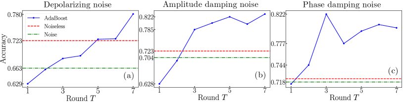
Figure 5: Prediction accuracy of variational quantum AdaBoost in the presence of noise. (a) QCNN with depolarizing noise. (b) QCNN with amplitude damping noise. (c) QCNN with phase damping noise. The blue solid line depicts the performance of variational quantum AdaBoost. The green dash-dotted line describes the prediction accuracy of the classifier employing the noisy QCNN, while the red dashed line depicts that with the ideally noiseless QCNN. Both of them do not take boosting operation. Variational quantum AdaBoost outperforms the noiseless classifier after at most $5$ rounds of boosting implying that AdaBoost can help mitigate the impact of different kinds of noise.

In addition, we investigate the performance of variational quantum AdaBoost in the presence of noise. In practice, single-qubit gates can be implemented with a high level of fidelity, while the fidelity of implementing $2$-qubit gates remains relatively lower. To take into account of this effect, we simulate a noisy $6$-qubit QCNN, and consider three typical classes of noises: depolarizing noise, amplitude damping noise, and phase damping noise. After each involved $2$-qubit gate we add a noise channel with noise probability $p=0.03$. We randomly sample two different $1000$-size sample sets for training and testing, respectively. For each sampled image, we first downsample it from $28\times 28$ to $8\times 8$ and then use the amplitude encoding to embed it into the QCNN. We illustrate the prediction accuracy of variational quantum AdaBoost in Fig. 5. For comparison, we also consider another two classifiers having no boosting operations. One (red dashed) is returned by using an ideally noiseless QCNN, and the other (green dash-dotted) is obtained by employing the noisy QCNN. For both of them, we optimize the PQC for at most $840$ iterations, which is the same number as that in $7$ rounds of variational quantum AdaBoost, and return the classifier having the best testing accuracy. The reason why their prediction accuracy is lower than that in Fig. 4 is that here we compress the images into $8\times 8$ format, while the images in Fig. 4 are compressed into $16\times 16$. Excessive compression leads to loss of information, thus reducing the overall prediction accuracy of the classifier. We find that for the three typical classes of noises, variational quantum AdaBoost outperforms the noiseless classifier after at most 5 rounds of boosting. This implies that AdaBoost can help mitigate the impact of different kinds of noises, which is particularly useful in the NISQ era. The reason is twofold. First, in variational quantum AdaBoost, weak classifiers can be boosted to obtain a strong classifier as long as the weak classifiers are slightly better than random guess. Noise may degrade the weak classifiers, however, as long as they are still better than random guess, they can be boosted to obtain a strong classifier. Second, as PQCs are shallow, quantum classifiers are weak, but also, the classifiers are less affected by noise due to shallow circuits.

IV Conclusion

In the current NISQ era, quantum machine learning usually involves a specification of a PQC and optimizing the trainable parameters in a classical fashion. Quantum machine learning has good generalization property while its trainability is generally poor. Ensemble methods are particularly appropriate to improve the trainability of quantum machine learning, and in turn help predict accurately. In this paper we theoretically establish the prediction guarantee of binary variational quantum AdaBoost, and numerically demonstrate that for multi-class classification problems, variational quantum AdaBoost not only can achieve high accuracy in prediction, but also help mitigate the impact of noise. For future work, it is interesting to incorporate ensemble methods to solve other practical tasks.

Appendix A Technical Lemmas

In this section, we present several lemmas that will be used in our proof of Theorem 1.

We first introduce a lemma that can be used to bound the training error of binary quantum AdaBoost.

Lemma 1.

(Theorem 7.2, [5]) The training error of the binary classifier returned by AdaBoost verifies:

$$\widehat{R}_{S}\left(f\right)\leq\exp{\left[-2\sum_{t=1}^{T}{{\left(\frac{1}{2}-\epsilon_{t}\right)}}^{2}\right]}.$$ (11)

Furthermore, if for all $t\in\left[T\right]$, $\epsilon_{t}\leq\frac{1}{2}-\gamma$, then

$$\widehat{R}_{S}\left(f\right)\leq e^{-2{\gamma}^{2}T}.$$ (12)

Then we recall a well-known result in machine learning which provides an upper bound on the generalization error.

Lemma 2.

(Theorem 3.3, [5]) Let $\mathcal{G}$ be a family of functions mapping from $\mathcal{Z}$ to $\left[0,1\right]$. Then, for any $\delta\,\textgreater\,0$, with probability at least $1-\delta$ over the draw of an i.i.d. sample set $S=\left\{z_{i}\right\}_{i=1}^{n}$ according to an unknown distribution $\mathcal{D}$, the following inequality holds for all $g\in\mathcal{G}$:

$$\mathop{\mathbb{E}}\limits_{z\sim\mathcal{D}}{\left[g\left(z\right)\right]}\leq\frac{1}{n}\sum_{i=1}^{n}{g\left(z_{i}\right)}+2\mathfrak{R}_{n}\left(\mathcal{G}\right)+\sqrt{\frac{\log{\frac{1}{\delta}}}{2n}},$$

where $\mathfrak{R}_{n}\left(\mathcal{G}\right)$ denotes the expectation of the empirical Rademacher complexity $\widehat{\mathfrak{R}}_{S}\left(\mathcal{G}\right)$ of $\mathcal{G}$, defined as

$$\mathfrak{R}_{n}\left(\mathcal{G}\right)=\mathop{\mathbb{E}}\limits_{S\sim{\mathcal{D}}^{n}}\left[\widehat{\mathfrak{R}}_{S}\left(\mathcal{G}\right)\right]=\mathop{\mathbb{E}}\limits_{S\sim{\mathcal{D}}^{n}}{\mathop{\mathbb{E}}\limits_{\bm{\sigma}}{\left[\sup_{g\in\mathcal{G}}\frac{1}{n}\sum_{i=1}^{n}{\sigma_{i}g\left(z_{i}\right)}\right],}}$$ (13)

where $\bm{\sigma}=\left(\sigma_{1},\cdots,\sigma_{n}\right)^{\top}$, with $\sigma_{i}$s independent uniform random variables taking values in $\left\{-1,+1\right\}$.

The following lemma relates the empirical Rademacher complexity of a new set of composite functions of a hypothesis in $\mathcal{H}$ and a Lipschitz function to the empirical Rademacher complexity of the hypothesis set $\mathcal{H}$.

Lemma 3.

(Lemma 5.7, [5]) Let $\Phi_{1},\cdots,\Phi_{n}$ be $l$-Lipschitz functions from $\mathbb{R}$ to $\mathbb{R}$ and $\bm{\sigma}=\left(\sigma_{1},\cdots,\sigma_{n}\right)^{\top}$ with $\sigma_{i}$s independent uniform random variables taking values in $\left\{-1,+1\right\}$. Then, for any hypothesis set $\mathcal{H}$ of real-valued functions, the following inequality holds:

$$\frac{1}{n}\mathop{\mathbb{E}}\limits_{\bm{\sigma}}{\left[\sup_{h\in\mathcal{H}}\sum_{i=1}^{n}{\sigma_{i}\left(\Phi_{i}\circ h\right)\left(x_{i}\right)}\right]}\leq\frac{l}{n}\mathop{\mathbb{E}}\limits_{\bm{\sigma}}{\left[\sup_{h\in\mathcal{H}}\sum_{i=1}^{n}{\sigma_{i}h\left(x_{i}\right)}\right]}.$$

In our work, the hypothesis set $\mathcal{H}=\left\{h_{\bm{\theta}}:\bm{\theta}\in{\left[0,2\pi\right]}^{K}\right\}$, which is composed of PQC-based hypothesis $h_{\bm{\theta}}$ defined in the form of Eq. (7). We provide an upper bound of its Rademacher complexity in the following lemma (see Appendix C for a detailed proof).

Lemma 4.

For the quantum hypothesis set $\mathcal{H}=\left\{h_{\bm{\theta}}:\bm{\theta}\in{\left[0,2\pi\right]}^{K}\right\}$ with $h_{\bm{\theta}}$ being defined as in Eq. (7), its Rademacher complexity can be upper bounded by a function of the number of independent trainable quantum gates $K$ and the sample size $n$:

$$\mathfrak{R}_{n}\left(\mathcal{H}\right)\leq 6\sqrt{\frac{K\log 7K}{n}}+2\sqrt{\frac{K}{n}}.$$ (14)

Appendix B Proof of Theorem 1

Proof.

From Eqs. (3) and (8), it is straightforward to verify that evaluating the prediction error of the binary quantum AdaBoost classifier returned by Algorithm 2 is equivalent to evaluating $R\left(f\right)$ with $f=\sum_{t=1}^{T}{\alpha_{t}h_{t}}$ without the sign function.

Note that the quantum hypothesis set $\mathcal{H}=\left\{h_{\bm{\theta}}:\bm{\theta}\in{\left[0,2\pi\right]}^{K}\right\}$ is composed of $h_{\bm{\theta}}$ being defined as in Eq. (7), with range belonging to $\left[-1,1\right]$. Thus, in general, $f=\sum_{t=1}^{T}{\alpha_{t}h_{t}}$ does not belong to $\mathcal{H}$ or its convex hull which is defined as

$${\rm conv}\left(\mathcal{H}\right)=\left\{\sum_{k=1}^{p}{\mu_{k}h_{k}}:p\geq 1,\mu_{k}\geq 0,h_{k}\in\mathcal{H},\sum_{k=1}^{p}{\mu_{k}}\leq 1\right\}.$$ (15)

However, we can consider the normalized version of $f$, denoted by

$$\bar{f}=\frac{f}{\|\alpha\|_{1}}=\frac{f}{\sum_{t=1}^{T}{\alpha_{t}}},$$ (16)

which belongs to the convex hull of $\mathcal{H}$. Moreover, since $\text{sgn}\left(f\right)=\text{sgn}\left(\bar{f}\right)$, from Eqs. (3) and (8), we have

$$R\left(f\right)=R\left(\bar{f}\right),~{}\text{and}~{}\widehat{R}_{S}\left(f\right)=\widehat{R}_{S}\left(\bar{f}\right).$$ (17)

To bound $R\left(\bar{f}\right)$, let

$$\mathcal{G}=\left\{\mathbb{I}_{y\bar{f}\left(\bm{x}\right)\leq 0}:\left(\rho\left(\bm{x}\right),y\right)\in\mathcal{X}\times\mathcal{Y},\,\bar{f}=\frac{\sum_{t=1}^{T}{\alpha_{t}h_{t}}}{\|\alpha\|_{1}},\,h_{t}\in\mathcal{H},\,t\in\left[T\right]\right\}.$$ (18)

Then according to Lemma 2, it yields

$$R\left(\bar{f}\right)\leq\widehat{R}_{S}\left(\bar{f}\right)+2\mathfrak{R}_{n}\left(\mathcal{G}\right)+\sqrt{\frac{\log{\frac{1}{\delta}}}{2n}}.$$ (19)

Since the zero-one loss function is 1-Lipschitz, from Lemma 3, we have

$$\mathfrak{R}_{n}\left(\mathcal{G}\right)\leq\mathfrak{R}_{n}\left({\rm conv}\left(\mathcal{H}\right)\right).$$ (20)

Moreover, according to Lemma 7.4 in [5],

$$\mathfrak{R}_{n}\left({\rm conv}\left(\mathcal{H}\right)\right)=\mathfrak{R}_{n}\left(\mathcal{H}\right).$$ (21)

Now we can combine Eqs. (17), (19)-(21) to yield

$$R\left(f\right)\leq\widehat{R}_{S}\left(f\right)+2\mathfrak{R}_{n}\left(\mathcal{H}\right)+\sqrt{\frac{\log{\frac{1}{\delta}}}{2n}}.$$ (22)

Thus, if for all $t\in\left[T\right]$, $\epsilon_{t}\leq\frac{1}{2}-\gamma$, we can derive Theorem 1 by leveraging Lemma 1 and Lemma 4 to further bound Eq. (22). ∎

Appendix C Proof of Lemma 4

We first introduce the notion of covering number, which is a complexity measure that has been widely used in machine learning.

Definition 1.

(Covering nets and covering numbers [71]) Let $\left(\mathcal{H},d\right)$ be a metric space. Consider a subset $\mathcal{K}\subset\mathcal{H}$ and let $\epsilon\textgreater 0$. A subset $\mathcal{N}\subseteq\mathcal{K}$ is called an $\epsilon$-net of $\mathcal{K}$ if every point in $\mathcal{K}$ is within a distance $\epsilon$ of some point of $\mathcal{N}$, i.e.,

$$\forall~{}x\in\mathcal{K},\,\exists~{}y\in\mathcal{N}:~{}d\left(x,y\right)\leq\epsilon.$$

The smallest possible cardinality of an $\epsilon$-net of $\mathcal{K}$ is called the covering number of $\mathcal{K}$, and is denoted by $N\left(\mathcal{K},\epsilon,d\right)$.

For example, for Euclidean space $\left(\mathbb{R}^{K},\|\cdot\|_{\infty}\right)$, the covering number $N\left(\left[-\pi,\pi\right]^{K},\epsilon,\|\cdot\|_{\infty}\right)$ is equal to ${\lceil\pi/\epsilon\rceil}^{K}$, where $\lceil\cdot\rceil$ denotes the rounding up function. Intuitively, the hypercube $\left[-\pi,\pi\right]^{K}$ can be covered by a number of ${\lceil\pi/\epsilon\rceil}^{K}$ $K$-dimensional hypercubes whose sides have the same length $2\epsilon$.

Then we introduce several technical lemmas that will be used in the proof of Lemma 4.

The following lemma relates the distance between two unitary operators measured by the spectral norm to the distance between their corresponding unitary channels measured by the diamond norm.

Lemma 5.

(Lemma 4, Supplementary Information for [31]) Let $\mathcal{U}\left(\rho\right)=U\rho U^{{\dagger}}$ and $\mathcal{V}\left(\rho\right)=V\rho V^{{\dagger}}$ be unitary channels. Then,

$$\frac{1}{2}\|\mathcal{U}-\mathcal{V}\|_{\diamond}\leq\|U-V\|.$$

Here, $\|\cdot\|$ denotes the spectral norm, and the diamond norm of a quantum unitary channel $\mathcal{U}$ is defined as

$$\|\mathcal{U}\|_{\diamond}=\mathop{\max}\limits_{\left|\psi\rangle\langle\psi\right|}\|\mathcal{U}\left(\left|\psi\rangle\langle\psi\right|\right)\|_{1},$$

with $\|A\|_{1}={\rm Tr}\left[\sqrt{A^{\dagger}A}\right]$ being the trace norm.

The following lemma translates the distance between $J$-qubit rotational operators to the distance of their corresponding angles.

Lemma 6.

(Distance between rotational operators) Given an arbitrary $J$-qubit Pauli tensor product $P\in{\left\{I,X,Y,Z\right\}}^{\otimes J}$ and two arbitrary angles $\theta,\tilde{\theta}\in\left[0,2\pi\right]$, the corresponding $J$-qubit rotational operators are $R\left(\theta\right)=e^{-i\frac{\theta}{2}P}$ and $R\left(\tilde{\theta}\right)=e^{-i\frac{\tilde{\theta}}{2}P}$, respectively. Then, the distance between the two operators measured by the spectral norm can be upper bounded as

$$\Big{\|}R\left(\theta\right)-R\left(\tilde{\theta}\right)\Big{\|}\leq\frac{1}{2}\lvert\theta-\tilde{\theta}\rvert.$$

Proof.

According to the definition of rotational operators, we have

$$R\left(\theta\right)-R\left(\tilde{\theta}\right)=\left(\cos\frac{\theta}{2}-\cos\frac{\tilde{\theta}}{2}\right)I^{\otimes J}-i\left(\sin\frac{\theta}{2}-\sin\frac{\tilde{\theta}}{2}\right)P,$$

whose singular value is $2\left|\sin\frac{\theta-\tilde{\theta}}{4}\right|$ with $2^{J}$ multiplicity. Thus,

$$\Big{\|}R\left(\theta\right)-R\left(\tilde{\theta}\right)\Big{\|}=2\left|\sin\frac{\theta-\tilde{\theta}}{4}\right|\leq\frac{1}{2}\lvert\theta-\tilde{\theta}\rvert.$$

∎

In the main text, we only consider the ideally unitary channel for simplicity, namely, the PQC-based hypothesis is in the form of $h_{\bm{\theta}}\left(\bm{x}\right)={\rm Tr}\left[ZU\left(\bm{\theta}\right)\rho\left(\bm{x}\right)U^{\dagger}\left(\bm{\theta}\right)\right]$. To describe the noise effect, a general quantum channel $\mathcal{A}$ is defined by a linear map $\mathcal{A}:\mathcal{L}\left(\mathcal{H}_{A}\right)\rightarrow\mathcal{L}\left(\mathcal{H}_{B}\right)$, which is completely positive and trace preserving (CPTP). For a quantum channel $\mathcal{A}$, the diamond norm is defined as

$$\|\mathcal{A}\|_{\diamond}=\mathop{\sup}\limits_{\rho\in\mathcal{D}\left(\mathcal{H}_{RA}\right)}\|\left(\mathcal{I}_{R}\otimes\mathcal{A}\right)\left(\rho\right)\|_{1},$$

where $\mathcal{D}\left(\mathcal{H}_{RA}\right)$ denotes the set of density operators acting on the Hilbert space $\mathcal{H}_{RA}=\mathcal{H}_{R}\otimes\mathcal{H}_{A}$, and $\mathcal{I}_{R}$ is the identity map on the reference system $\mathcal{H}_{R}$, whose dimension can be arbitrary as long as the operator $\mathcal{I}_{R}\otimes\mathcal{A}$ is positive semi-definite.

The following lemma can help generalize the results of Lemma 4 and Theorem 1 from the case of unitary quantum channels described in the main text to those of noisy quantum channels. This means that the hypothesis functions can be generalized to

$$h_{\bm{\theta}}\left(\bm{x}\right)={\rm Tr}\left[Z\mathcal{E}_{\bm{\theta}}\left(\rho\left(\bm{x}\right)\right)\right],$$

where the noisy channel $\mathcal{E}_{\bm{\theta}}$ is composed of $K$ trainable multi-qubit rotational gates and arbitrarily many non-trainable gates. Notice that the general case can be reduced to the ideally unitary case by letting $\mathcal{E}_{\bm{\theta}}\left(\rho\right)=U\left(\bm{\theta}\right)\rho U^{{\dagger}}\left(\bm{\theta}\right)$.

Lemma 7.

(Subadditivity of diamond distance; Proposition 3.48, [72]) For any quantum channels $\mathcal{A}$, $\mathcal{B}$, $\mathcal{C}$, $\mathcal{D}$, where $\mathcal{B}$ and $\mathcal{D}$ map from $n$-qubit to $m$-qubit systems and $\mathcal{A}$ and $\mathcal{C}$ map from $m$-qubit to $k$-qubit systems, we have

$$\|\mathcal{A}\mathcal{B}-\mathcal{C}\mathcal{D}\|_{\diamond}\leq\|\mathcal{A}-\mathcal{C}\|_{\diamond}+\|\mathcal{B}-\mathcal{D}\|_{\diamond}.$$

The following lemma enables us to employ the covering number of one metric space to bound the covering number of another metric space.

Lemma 8.

(Covering numbers of two metric spaces; Lemma 3, [73]) Let $\left(\mathcal{H}_{1},d_{1}\right)$ and $\left(\mathcal{H}_{2},d_{2}\right)$ be two metric spaces and $f:\mathcal{H}_{1}\rightarrow\mathcal{H}_{2}$ be bi-Lipschitz such that

$$d_{2}\big{(}f\left(x\right),f\left(y\right)\big{)}\leq Kd_{1}\left(x,y\right),\forall~{}x,y\in\mathcal{H}_{1},$$

where $K$ is a constant. Then their covering numbers obey the following inequality as

$$N\left(\mathcal{H}_{2},\epsilon,d_{2}\right)\leq N\left(\mathcal{H}_{1},\epsilon/K,d_{1}\right).$$

According to the above lemmas, we can derive the covering number of general noisy quantum models.

Lemma 9.

(Covering number of noisy quantum models) If each element of $\bm{\theta}$ is selected from $\left[-\pi,\pi\right]$, then the covering number of the set of quantum channels $\left\{\mathcal{E}_{\bm{\theta}}\right\}$, each of which is composed of $K$ trainable multi-qubit rotational gates and arbitrarily many non-trainable quantum channels, can be upper bounded as

$$N\left(\mathcal{E}_{\bm{\theta}},\epsilon,\|\cdot\|_{\diamond}\right)\leq\bigg{\lceil}\frac{\pi K}{\epsilon}\bigg{\rceil}^{K}.$$

Proof.

From the structure of $\mathcal{E}_{\bm{\theta}}$, we have

$$\|\mathcal{E}_{\bm{\theta}}-\mathcal{E}_{\tilde{\bm{\theta}}}\|_{\diamond} \leq\sum_{k=1}^{K}{\Big{\|}\mathcal{R}_{k}\left(\theta_{k}\right)-\mathcal{R}_{k}\left(\tilde{\theta}_{k}\right)\Big{\|}_{\diamond}}$$ (23)

$$\leq 2\sum_{k=1}^{K}{\Big{\|}R_{k}^{\left(i_{k},j_{k}\right)}\left(\theta_{k}\right)-R_{k}^{\left(i_{k},j_{k}\right)}\left(\tilde{\theta}_{k}\right)}\Big{\|}$$ (24)

$$\leq\sum_{k=1}^{K}{\lvert\theta_{k}-\tilde{\theta}_{k}\rvert}$$ (25)

$$=\|\bm{\theta}-\tilde{\bm{\theta}}\|_{1}$$ (26)

$$\leq K\|\bm{\theta}-\tilde{\bm{\theta}}\|_{\infty},$$ (27)

where $\mathcal{R}_{k}\left(\theta_{k}\right)$ denotes the quantum channel corresponding to the $J$-qubit rotational operator $R_{k}^{\left(i_{k},j_{k}\right)}\left(\theta_{k}\right)$. Here, Eq. (23) is derived by repeatedly using Lemma 7 to erase the non-trainable quantum channels, Eqs. (24) and (25) are obtained from Lemma 5 and Lemma 6, respectively, and Eq. (27) owes to the relation between the $l_{1}$-norm and $l_{\infty}$-norm for vectors in $\mathbb{R}^{K}$.

Thus, according to Lemma 8, we have

$$N\left(\mathcal{E}_{\bm{\theta}},\epsilon,\|\cdot\|_{\diamond}\right)\leq N\left(\bm{\theta},\frac{\epsilon}{K},\|\cdot\|_{\infty}\right)=\bigg{\lceil}\frac{\pi K}{\epsilon}\bigg{\rceil}^{K}.$$

∎

Now we prove Lemma 4 by leveraging the technique of proving Theorem 6 in Supplementary Information of [31].

Proof.

To bound the Rademacher complexity

$$\mathfrak{R}_{n}\left(\mathcal{H}\right)=\mathop{\mathbb{E}}\limits_{S\sim{\mathcal{D}}^{n}}{\mathop{\mathbb{E}}\limits_{\bm{\sigma}}{\left[\sup_{h_{\bm{\theta}}\in\mathcal{H}}\frac{1}{n}\sum_{i=1}^{n}{\sigma_{i}h_{\bm{\theta}}\left(\bm{x}_{i}\right)}\right]}},$$

the main idea is to use the chaining technique to bound the empirical Rademacher complexity

$$\mathop{\mathbb{E}}\limits_{\bm{\sigma}}{\left[\sup_{h_{\bm{\theta}}\in\mathcal{H}}\frac{1}{n}\sum_{i=1}^{n}{\sigma_{i}h_{\bm{\theta}}\left(\bm{x}_{i}\right)}\right]}$$

in terms of covering number.

First, with respect to the diamond norm, for each $j\in\mathbb{N}_{0}$, there exists an $2^{-j}$-covering net denoted by $\mathcal{N}_{j}$ for the set of quantum channels $\left\{\mathcal{E}_{\bm{\theta}}\right\}$, satisfying $N_{j}\leq\big{\lceil}2^{j}\pi K\big{\rceil}^{K}$. To be specific, for each $j\in\mathbb{N}$ and every parameter setting $\bm{\theta}$, there exists a quantum operator $\mathcal{E}_{\bm{\theta},j}\in\mathcal{N}_{j}$ such that

$$\|\mathcal{E}_{\bm{\theta}}-\mathcal{E}_{\bm{\theta},j}\|_{\diamond}\leq\frac{1}{2^{j}}.$$

For $j=0$, the $1$-covering net of $\left\{\mathcal{E}_{\bm{\theta}}\right\}$ is $\mathcal{N}_{0}=\left\{0\right\}$. Moreover, according to Lemma 9, the covering number $N_{j}$ can be upper bounded by $\big{\lceil}2^{j}\pi K\big{\rceil}^{K}$ .

Then, for any $k\in\mathbb{N}$, we have

$$\mathcal{E}_{\bm{\theta}}=\mathcal{E}_{\bm{\theta}}-\mathcal{E}_{\bm{\theta},k}+\sum_{j=k}^{1}{\mathcal{E}_{\bm{\theta},j}-\mathcal{E}_{\bm{\theta},j-1}},$$

and

$$\mathop{\mathbb{E}}\limits_{\bm{\sigma}}{\left[\sup_{h_{\bm{\theta}}\in\mathcal{H}}\frac{1}{n}\sum_{i=1}^{n}{\sigma_{i}h_{\bm{\theta}}\left(\bm{x}_{i}\right)}\right]}= \mathop{\mathbb{E}}\limits_{\bm{\sigma}}{\left[\sup_{h_{\bm{\theta}}\in\mathcal{H}}\frac{1}{n}\sum_{i=1}^{n}{\sigma_{i}{\rm Tr}\left[Z\mathcal{E}_{\bm{\theta}}\left(\rho\left(\bm{x}_{i}\right)\right)\right]}\right]}$$

$$\leq \frac{1}{2^{k}}+\frac{6}{\sqrt{n}}\sum_{j=1}^{k}{\frac{1}{2^{j}}\sqrt{\log N_{j}}}$$ (28)

$$\leq \frac{1}{2^{k}}+\frac{6}{\sqrt{n}}\sum_{j=1}^{k}{\frac{1}{2^{j}}\sqrt{K\log\lceil 2^{j}\pi K\rceil}}$$ (29)

$$\leq \frac{1}{2^{k}}+12\sqrt{\frac{K}{n}}\int_{\frac{1}{2^{\left(k+1\right)}}}^{\frac{1}{2}}{\sqrt{\log\bigg{\lceil}\frac{\pi K}{\alpha}\bigg{\rceil}}}{\rm d}\alpha,$$ (30)

$$\leq \frac{1}{2^{k}}+12\sqrt{\frac{K}{n}}\int_{\frac{1}{2^{\left(k+1\right)}}}^{\frac{1}{2}}{\sqrt{\log\frac{7K}{2\alpha}}}{\rm d}\alpha,$$ (31)

where Eq. (28) is derived following a similar analysis as that in Supplementary Information of [31].

By taking the limit $k\rightarrow\infty$, we obtain

$$\mathop{\mathbb{E}}\limits_{\bm{\sigma}}{\left[\sup_{h_{\bm{\theta}}\in\mathcal{H}}\frac{1}{n}\sum_{i=1}^{n}{\sigma_{i}h_{\bm{\theta}}\left(\bm{x}_{i}\right)}\right]}\leq\, 12\sqrt{\frac{K}{n}}\int_{0}^{\frac{1}{2}}{\sqrt{\log\frac{7K}{2\alpha}}}{\rm d}\alpha$$ (32)

$$=\, 12\sqrt{\frac{K}{n}}\left[\frac{\sqrt{\log 7K}}{2}+\frac{7\sqrt{\pi}K}{4}{\rm erfc}\left(\sqrt{\log 7K}\right)\right],$$ (33)

$$\leq\, 6\sqrt{\frac{K\log 7K}{n}}+2\sqrt{\frac{K}{n}},$$ (34)

where Eq. (33) is derived by using the integral

$$\int{\sqrt{\log\frac{1}{\alpha}}}{\rm d}\alpha=\alpha\sqrt{\log\frac{1}{\alpha}}-\frac{\sqrt{\pi}}{2}{\rm erf}\left(\sqrt{\log\frac{1}{\alpha}}\right),$$ (35)

with the error function defined by ${\rm erf}\left(x\right)=\frac{2}{\sqrt{\pi}}\int_{0}^{x}{e^{-t^{2}}}{\rm d}t$ and the complementary error function ${\rm erfc}\left(x\right)=1-{\rm erf}\left(x\right)$. Besides, we notice that the function $K{\rm erfc}\left(\sqrt{\log 7K}\right)$ decreases monotonically with $K\in\mathbb{N}$ and is upper bounded by ${\rm erfc}\left(\sqrt{\log 7}\right)\leq 0.0486$, so we have Eq. (34).

Thus, by taking expectations of both sides of Eq. (34) over the training sample set $S$, we have Eq. (14). ∎

References

- Krenn et al. [2023] M. Krenn, J. Landgraf, T. Foesel, and F. Marquardt, Artificial intelligence and machine learning for quantum technologies, Phys. Rev. A 107, 010101 (2023).
- Lu et al. [2018] S. Lu, S. Huang, K. Li, J. Li, J. Chen, D. Lu, Z. Ji, Y. Shen, D. Zhou, and B. Zeng, Separability-entanglement classifier via machine learning, Phys. Rev. A 98, 012315 (2018).
- Luo et al. [2023] Y.-J. Luo, J.-M. Liu, and C. Zhang, Detecting genuine multipartite entanglement via machine learning, Phys. Rev. A 108, 052424 (2023).
- Shingu et al. [2021] Y. Shingu, Y. Seki, S. Watabe, S. Endo, Y. Matsuzaki, S. Kawabata, T. Nikuni, and H. Hakoshima, Boltzmann machine learning with a variational quantum algorithm, Phys. Rev. A 104, 032413 (2021).
- Mohri et al. [2018] M. Mohri, A. Rostamizadeh, and A. Talwalkar, Foundations of machine learning (MIT press, 2018).
- Wright and Ma [2022] J. Wright and Y. Ma, High-dimensional data analysis with low-dimensional models: Principles, computation, and applications (Cambridge University Press, 2022).
- Rasmussen and Ghahramani [2000] C. Rasmussen and Z. Ghahramani, Occam’s razor, Adv. Neural Inf. Process. 13 (2000).
- Li et al. [2018] H. Li, Z. Xu, G. Taylor, C. Studer, and T. Goldstein, Visualizing the loss landscape of neural nets, Adv. Neural Inf. Process. 31 (2018).
- Geiger et al. [2021] M. Geiger, L. Petrini, and M. Wyart, Landscape and training regimes in deep learning, Phys. Rep. 924, 1 (2021).
- Rocks and Mehta [2022] J. W. Rocks and P. Mehta, Memorizing without overfitting: Bias, variance, and interpolation in overparameterized models, Phys. Rev. Res. 4, 013201 (2022).
- Baldassi et al. [2022] C. Baldassi, C. Lauditi, E. M. Malatesta, R. Pacelli, G. Perugini, and R. Zecchina, Learning through atypical phase transitions in overparameterized neural networks, Phys. Rev. E 106, 014116 (2022).
- Allen-Zhu et al. [2019] Z. Allen-Zhu, Y. Li, and Z. Song, A convergence theory for deep learning via over-parameterization, in ICML (2019) pp. 242–252.
- Larocca et al. [2023] M. Larocca, N. Ju, D. García-Martín, P. J. Coles, and M. Cerezo, Theory of overparametrization in quantum neural networks, Nat. Comput. Sci. 3, 542 (2023).
- Biamonte et al. [2017] J. Biamonte, P. Wittek, N. Pancotti, P. Rebentrost, N. Wiebe, and S. Lloyd, Quantum machine learning, Nature 549, 195 (2017).
- Beer et al. [2023] K. Beer, M. Khosla, J. Köhler, T. J. Osborne, and T. Zhao, Quantum machine learning of graph-structured data, Phys. Rev. A 108, 012410 (2023).
- Uvarov et al. [2020] A. Uvarov, A. Kardashin, and J. D. Biamonte, Machine learning phase transitions with a quantum processor, Phys. Rev. A 102, 012415 (2020).
- Banchi et al. [2021] L. Banchi, J. Pereira, and S. Pirandola, Generalization in quantum machine learning: A quantum information standpoint, PRX Quantum 2, 040321 (2021).
- Cerezo et al. [2022] M. Cerezo, G. Verdon, H.-Y. Huang, L. Cincio, and P. J. Coles, Challenges and opportunities in quantum machine learning, Nat. Comput. Sci. 2, 567 (2022).
- Benedetti et al. [2019a] M. Benedetti, E. Lloyd, S. Sack, and M. Fiorentini, Parameterized quantum circuits as machine learning models, Quantum Sci. Technol. 4, 043001 (2019a).
- Schuld et al. [2021] M. Schuld, R. Sweke, and J. J. Meyer, Effect of data encoding on the expressive power of variational quantum-machine-learning models, Phys. Rev. A 103, 032430 (2021).
- Liu et al. [2021] Y. Liu, S. Arunachalam, and K. Temme, A rigorous and robust quantum speed-up in supervised machine learning, Nat. Phys 17, 1013 (2021).
- Albrecht et al. [2023] B. Albrecht, C. Dalyac, L. Leclerc, L. Ortiz-Gutiérrez, S. Thabet, M. D’Arcangelo, J. R. K. Cline, V. E. Elfving, L. Lassablière, H. Silvério, B. Ximenez, L.-P. Henry, A. Signoles, and L. Henriet, Quantum feature maps for graph machine learning on a neutral atom quantum processor, Phys. Rev. A 107, 042615 (2023).
- Huang et al. [2022] H.-Y. Huang, M. Broughton, J. Cotler, S. Chen, J. Li, M. Mohseni, H. Neven, R. Babbush, R. Kueng, J. Preskill, et al., Quantum advantage in learning from experiments, Science 376, 1182 (2022).
- Jerbi et al. [2023] S. Jerbi, L. J. Fiderer, et al., Quantum machine learning beyond kernel methods, Nat. Commun. 14, 517 (2023).
- Cerezo et al. [2021a] M. Cerezo, A. Arrasmith, R. Babbush, S. C. Benjamin, S. Endo, K. Fujii, J. R. McClean, K. Mitarai, X. Yuan, L. Cincio, et al., Variational quantum algorithms, Nat. Rev. Phys. 3, 625 (2021a).
- Benedetti et al. [2019b] M. Benedetti, E. Lloyd, S. Sack, and M. Fiorentini, Parameterized quantum circuits as machine learning models, Quantum Sci. Technol. 4, 043001 (2019b).
- Havlíček et al. [2019] V. Havlíček, A. D. Córcoles, K. Temme, A. W. Harrow, A. Kandala, J. M. Chow, and J. M. Gambetta, Supervised learning with quantum-enhanced feature spaces, Nature 567, 209 (2019).
- Schuld and Killoran [2019] M. Schuld and N. Killoran, Quantum machine learning in feature hilbert spaces, Phys. Rev. Lett. 122, 040504 (2019).
- Pérez-Salinas et al. [2020] A. Pérez-Salinas, A. Cervera-Lierta, E. Gil-Fuster, and J. I. Latorre, Data re-uploading for a universal quantum classifier, Quantum 4, 226 (2020).
- Wang et al. [2024] Y. Wang, B. Qi, X. Wang, T. Liu, and D. Dong, Power characterization of noisy quantum kernels, arXiv preprint arXiv:2401.17526 (2024).
- Caro et al. [2022] M. C. Caro, H.-Y. Huang, M. Cerezo, K. Sharma, A. Sornborger, L. Cincio, and P. J. Coles, Generalization in quantum machine learning from few training data, Nat. Commun. 13, 4919 (2022).
- McClean et al. [2018] J. R. McClean, S. Boixo, V. N. Smelyanskiy, R. Babbush, and H. Neven, Barren plateaus in quantum neural network training landscapes, Nat. Commun. 9, 4812 (2018).
- Haug et al. [2021] T. Haug, K. Bharti, and M. Kim, Capacity and quantum geometry of parametrized quantum circuits, PRX Quantum 2, 040309 (2021).
- Cerezo et al. [2021b] M. Cerezo, A. Sone, T. Volkoff, L. Cincio, and P. J. Coles, Cost function dependent barren plateaus in shallow parametrized quantum circuits, Nat. Commun. 12, 1 (2021b).
- Marrero et al. [2021] C. O. Marrero, M. Kieferová, and N. Wiebe, Entanglement-induced barren plateaus, PRX Quantum 2, 040316 (2021).
- Zhao and Gao [2021] C. Zhao and X.-S. Gao, Analyzing the barren plateau phenomenon in training quantum neural networks with the ZX-calculus, Quantum 5, 466 (2021).
- Wang et al. [2023a] Y. Wang, B. Qi, C. Ferrie, and D. Dong, Trainability enhancement of parameterized quantum circuits via reduced-domain parameter initialization, arXiv preprint arXiv:2302.06858 (2023a).
- Wang et al. [2023b] X. Wang, B. Qi, Y. Wang, and D. Dong, EHA: Entanglement-variational hardware-efficient ansatz for eigensolvers, arXiv preprint arXiv:2311.01120 (2023b).
- Anschuetz and Kiani [2022] E. R. Anschuetz and B. T. Kiani, Quantum variational algorithms are swamped with traps, Nat. Commun. 13, 7760 (2022).
- You and Wu [2021] X. You and X. Wu, Exponentially many local minima in quantum neural networks, in ICML (2021) pp. 12144–12155.
- Breiman [1996] L. Breiman, Bagging predictors, Mach. Learn. 24, 123 (1996).
- Lam and Suen [1997] L. Lam and S. Suen, Application of majority voting to pattern recognition: an analysis of its behavior and performance, IEEE Trans. Syst. Man Cybern. 27, 553 (1997).
- Lin et al. [2003] X. Lin, S. Yacoub, J. Burns, and S. Simske, Performance analysis of pattern classifier combination by plurality voting, Pattern Recognit. Lett. 24, 1959 (2003).
- Schapire et al. [1999] R. E. Schapire et al., A brief introduction to boosting, in IJCAI, Vol. 99 (Citeseer, 1999) pp. 1401–1406.
- Jiang et al. [2020] Y. Jiang, B. Neyshabur, H. Mobahi, D. Krishnan, and S. Bengio, Fantastic generalization measures and where to find them, in ICLR (2020).
- McAllester [1999] D. A. McAllester, PAC-Bayesian model averaging, in COLT (1999) pp. 164–170.
- Freund and Schapire [1997] Y. Freund and R. E. Schapire, A decision-theoretic generalization of on-line learning and an application to boosting, J. Comput. Syst. Sci. 55, 119 (1997).
- Bartlett et al. [1998] P. Bartlett, Y. Freund, W. S. Lee, and R. E. Schapire, Boosting the margin: A new explanation for the effectiveness of voting methods, Ann. Math. Stat. 26, 1651 (1998).
- Grønlund et al. [2019] A. Grønlund, L. Kamma, K. Green Larsen, A. Mathiasen, and J. Nelson, Margin-based generalization lower bounds for boosted classifiers, Adv. Neural Inf. Process. 32 (2019).
- Sun et al. [2021] K. Sun, Z. Zhu, and Z. Lin, AdaGCN: Adaboosting graph convolutional networks into deep models, in ICLR (2021).
- Drucker et al. [1993] H. Drucker, R. Schapire, and P. Simard, Boosting performance in neural networks, IJPRAI 7, 705 (1993).
- Li et al. [2008] X. Li, L. Wang, and E. Sung, AdaBoost with SVM-based component classifiers, Eng. Appl. Artif. Intell. 21, 785 (2008).
- Zhang et al. [2019] Y. Zhang, M. Ni, C. Zhang, S. Liang, S. Fang, R. Li, and Z. Tan, Research and application of AdaBoost algorithm based on SVM, in ITAIC (IEEE, 2019) pp. 662–666.
- Arunachalam and Maity [2020] S. Arunachalam and R. Maity, Quantum boosting, in ICML (2020) pp. 377–387.
- Wang et al. [2021] X. Wang, Y. Ma, M.-H. Hsieh, and M.-H. Yung, Quantum speedup in adaptive boosting of binary classification, Sci. CHINA. Phys. Mech. 64, 220311 (2021).
- Ohno [2022] H. Ohno, Boosting for quantum weak learners, Quantum Inf. Process. 21, 199 (2022).
- Li et al. [2024] Q. Li, Y. Huang, X. Hou, Y. Li, X. Wang, and A. Bayat, Ensemble-learning error mitigation for variational quantum shallow-circuit classifiers, Phys. Rev. Res. 6, 013027 (2024).
- Incudini et al. [2023] M. Incudini, M. Grossi, A. Ceschini, A. Mandarino, M. Panella, S. Vallecorsa, and D. Windridge, Resource saving via ensemble techniques for quantum neural networks, Quantum Mach. Intell. 5, 39 (2023).
- Goto et al. [2021] T. Goto, Q. H. Tran, and K. Nakajima, Universal approximation property of quantum machine learning models in quantum-enhanced feature spaces, Phys. Rev. Lett. 127, 090506 (2021).
- Lloyd et al. [2020] S. Lloyd, M. Schuld, A. Ijaz, J. Izaac, and N. Killoran, Quantum embeddings for machine learning, arXiv preprint arXiv:2001.03622 (2020).
- Hastie et al. [2009] T. Hastie, S. Rosset, J. Zhu, and H. Zou, Multi-class AdaBoost, Stat. Interface 2, 349 (2009).
- LeCun et al. [1998] Y. LeCun, L. Bottou, Y. Bengio, and P. Haffner, Gradient-based learning applied to document recognition, Proceedings of the IEEE 86, 2278 (1998).
- Pesah et al. [2021] A. Pesah, M. Cerezo, S. Wang, T. Volkoff, A. T. Sornborger, and P. J. Coles, Absence of barren plateaus in quantum convolutional neural networks, Phys. Rev. X 11, 041011 (2021).
- Wei et al. [2022] S. Wei, Y. Chen, Z. Zhou, and G. Long, A quantum convolutional neural network on nisq devices, AAPPS Bulletin 32, 1 (2022).
- Chen et al. [2022] S. Y.-C. Chen, T.-C. Wei, C. Zhang, H. Yu, and S. Yoo, Quantum convolutional neural networks for high energy physics data analysis, Phys. Rev. Res. 4, 013231 (2022).
- Hur et al. [2022] T. Hur, L. Kim, and D. K. Park, Quantum convolutional neural network for classical data classification, Quantum Mach. Intell. 4, 3 (2022).
- Kingma and Ba [2014] D. P. Kingma and J. Ba, Adam: A method for stochastic optimization, arXiv preprint arXiv:1412.6980 (2014).
- Romero et al. [2018] J. Romero, R. Babbush, J. R. McClean, C. Hempel, P. J. Love, and A. Aspuru-Guzik, Strategies for quantum computing molecular energies using the unitary coupled cluster ansatz, Quantum Sci. Technol. 4, 014008 (2018).
- Mitarai et al. [2018] K. Mitarai, M. Negoro, M. Kitagawa, and K. Fujii, Quantum circuit learning, Phys. Rev. A 98, 032309 (2018).
- Schuld et al. [2019] M. Schuld, V. Bergholm, C. Gogolin, J. Izaac, and N. Killoran, Evaluating analytic gradients on quantum hardware, Phys. Rev. A 99, 032331 (2019).
- Dudley [2014] R. M. Dudley, Uniform central limit theorems, Vol. 142 (Cambridge university press, 2014).
- Watrous [2018] J. Watrous, The theory of quantum information (Cambridge university press, 2018).
- Barthel and Lu [2018] T. Barthel and J. Lu, Fundamental limitations for measurements in quantum many-body systems, Phys. Rev. Lett. 121, 080406 (2018).