AutoTimes: Autoregressive Time Series Forecasters via Large Language Models

Abstract

Foundation models of time series have not been fully developed due to the limited availability of large-scale time series and the underexploration of scalable pre-training. Based on the similar sequential structure of time series and natural language, increasing research demonstrates the feasibility of leveraging large language models (LLM) for time series. Nevertheless, prior methods may overlook the consistency in aligning time series and natural language, resulting in insufficient utilization of the LLM potentials. To fully exploit the general-purpose token transitions learned from language modeling, we propose AutoTimes to repurpose LLMs as Autoregressive Time series forecasters, which is consistent with the acquisition and utilization of LLMs without updating the parameters. The consequent forecasters can handle flexible series lengths and achieve competitive performance as prevalent models. Further, we present token-wise prompting that utilizes corresponding timestamps to make our method applicable to multimodal scenarios. Analysis demonstrates our forecasters inherit zero-shot and in-context learning capabilities of LLMs. Empirically, AutoTimes exhibits notable method generality and achieves enhanced performance by basing on larger LLMs, additional texts, or time series as instructions.

1 Introduction

Time series forecasting is of crucial demand in real-world applications, covering diverse domains including climate, economics, energy, operations, etc (Liu et al., 2023c). The growing need for ubiquitous forecasting scenarios, where time series observations are scarce or the forecasting can be instructed by auxiliary information in other modalities (Xue & Salim, 2023; Woo et al., 2023), underscores the demand for the foundation models (Bommasani et al., 2021) of time series, which exhibits the enhanced capabilities, including zero-shot generalization, in-context learning (Brown et al., 2020), emergent abilities (Wei et al., 2022) and multimodal utilization (OpenAI, 2023), thereby expanding the scope of time series forecasting to a wider range of situations.

However, the development of time series foundation models has been impeded by the limited availability of large-scale datasets for pre-training and the uncertainty of techniques for developing large time series models. In contrast, we are witnessing rapid progress in large language models (LLM), facilitated by extensive text corpora (Zhu et al., 2015), the prevalence of pre-trained models (Touvron et al., 2023), and well-established adaptation techniques (Hu et al., 2021). Notably, language modeling and time series forecasting share commonalities in sequential structure and autoregressive generation, presenting the opportunity to adopt off-the-shelf LLMs for time series without pre-training.

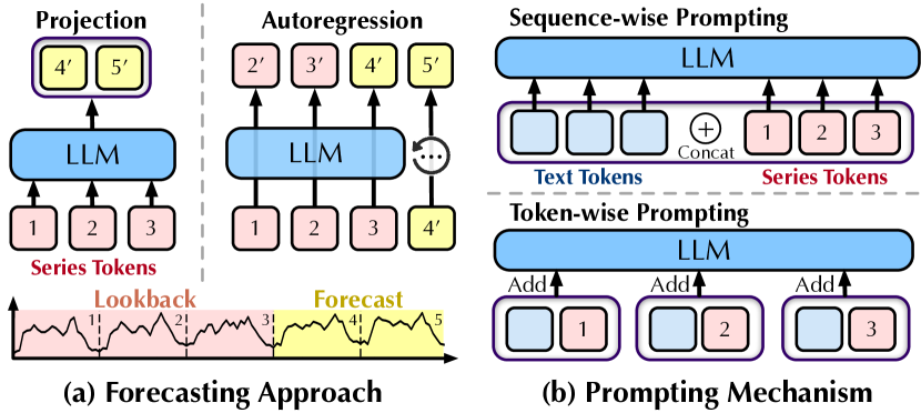
Figure 1: Illustration of LLM-repurposed forecasters to generate predictions and prompting mechanisms of text instructions.

Despite recent studies on large language models for time series (LLM4TS) achieving performance breakthroughs in the forecasting benchmarks (Jin et al., 2023), the mechanism by which LLMs adapt to the time series modality remains obscure. FPT (Zhou et al., 2023) hypothesizes a representation learning perspective, which leverages LLMs as generic sequential representation extractors, influencing subsequent LLM4TS methodologies. As depicted in Figure 1(a), segmented lookback series tokens are fed into the LLM, and the representations are directly projected for all predicted tokens in a single step. However, this perspective may lead to the collapse of token dependencies and contradict the mainstream structure of LLMs, the decoder-only architecture for autoregressive generation. Given that prior studies (Wang et al., 2022b; Dai et al., 2022) have demonstrated that the capabilities of zero-shot generalization and in-context learning are largely derived from the decoder-only design trained autoregressively, advantages of adapting LLMs for time series may not be fully realized until now. Furthermore, autoregression is aligned with the essential concept of statistical forecasters, for example, ARIMA (Box et al., 2015) and exponential smoothing (Winters, 1960), which empowers the model with the ability to handle arbitrary context length like LLMs, instantiated as one forecaster for variable lengths of the lookback and forecast window.

Based on the above reflections, we propose AutoTimes in this paper, which ensures the consistency to fully revitalize LLM capabilities to produce autoregressive forecasters as foundation models of time series. This consistency includes (1) training and inference: we adopt the consistent training objective with the LLM acquisition, i.e., the next token prediction (Bengio et al., 2000), to establish the tokenization of time series segments that encompass local series variations. During inference, we utilize the variable context length and autoregressive generation of LLMs to tackle arbitrary series lengths; (2) parameters: we leverage the token transitions of LLMs, which is parameterized by training on numerous text corpora, and apply it to time series tokens. Technically, we freeze the Transformer (Vaswani et al., 2017) layers of the repurposed LLM and establish the tokenizer and detokenizer of time series accounting for up to 0.1% total parameters. In addition to the improved efficiency of adaptation, it is aimed at achieving homeomorphic embeddings of time series that can be seamlessly mixed with texts at the token level. Based on it, we introduce token-wise prompting as shown in Figure 1(b), which takes advantage of the associated textual anchor of time series, the timestamp, to further enhance forecasting. While previous sequence-wise prompting concatenating different modalities can lead to an excessive sequence length and token disparities, our forecaster with the token-wise prompting and in-context learning as shown in Figure 4, can utilize both instructive texts and time series for a broader range of forecasting scenarios. Overall, our contributions can be summarized as follows:

• We delve into the modality alignment between time series and natural language to harness the token generation capability of LLMs as out-of-the-box forecasters.

• We propose AutoTimes, a simple but effective way to repurpose LLMs without altering any parameters, which tokenizes time series into the embedding space of LLMs and effectively leverages the inherent token transition to predict time series autoregressively.

• Compared with state-of-the-art approaches, our repurposed forecaster achieves competitive performance free from training on the specific series length, and further exhibits zero-shot generability, in-context learning, and multimodal utilizability empowered by LLMs.

2 Related Work

2.1 Autoregressive Models

Autoregression is the key concept of both language modeling and time series forecasting. Through revisiting the most classical autoregressive (AR) models, it becomes apparent that the AR model is the linear parameterization of language modeling when regarding time points as language tokens. While non-autoregressive forecasting has become the de-facto standard of prevalent deep forecasters binding with the encode-only structure (Wu et al., 2022; Nie et al., 2022; Das et al., 2023), the concept of autoregression serves as the fundamental principle for statistical forecasters, which enables these methods to applicable on variable lookback and forecast lengths. For stationary time series, the transition underlying the AR model remains invariant from the past to the future, which is the basis that the prediction can be made, as well as how ARIMA (Box, 2013) is developed by incorporating stationarization. Given prior knowledge, such as pre-assigned weights at specific time points, or separate modeling and correlating on time series components, methods such as exponential smoothing (Winters, 1960) and state space models (Durbin & Koopman, 2012) also take formulation based on the autoregressive generation.

Similar to language modeling based on the Markov assumption, the essence of autoregressive models lies in the invariant transition. Due to this, autoregressive models can excel at handling varying context length and long sequence generation, which is implemented by the decoder-only structure in terms of language models. However, drawing from the development of LLMs, the difficulty of training decoder-only architectures can be more significant than the encoder-only models, which necessitates a greater amount of training samples (Hoffmann et al., 2022). Still, the autoregressive training protocol coupled with the decoder-only structure also provides increased supervision, scalability (Brown et al., 2020), and better generalization (Wang et al., 2022b), thereby establishing it as the mainstream of LLMs (Zhao et al., 2023). Thus, it is imperative to adapt off-the-shelf LLMs as original autoregressive forecasters, which endow the potential to serve as foundational models for time series.

Table 1: Comparison between prior large language models for time series methods and our proposed AutoTimes.

Method	AutoTimes	TimeLLM	LLM4TS	FPT	UniTime	LLMTime	TEST	TEMPO	PromptCast
	(Ours)	(2023)	(2023)	(2023)	(2023b)	(2023)	(2023)	(2023)	(2023)
Autoregressive	✓	✗	✗	✗	✗	✓	✗	✗	✗
Freeze Parameters	✓	✓	✗	✗	✗	✓	✓	✗	✓
Multimodal	✓	✓	✗	✗	✓	✗	✓	✓	✓

2.2 Large Language Models for Time Series

With the immense advancement of large language model infrastructure, LLM4TS methods have been experiencing significant development in recent years. PromptCast (Xue & Salim, 2023) reformulates time series as text prompts and accomplishes forecasting as a sentence-to-sentence task. LLMTime (Gruver et al., 2023) delves into the encoding of time series as numerical tokens, demonstrating the scalability of LLMs on time series forecasting. FPT (Zhou et al., 2023) fine-tunes parameters of the LLM to adapt it as representation extractors serving for general time series analysis. LLM4TS (Chang et al., 2023) further introduces a two-stage fine-tuning protocol to activate language models on time series modality gradually. Based on thriving prompting techniques, specific templates (Liu et al., 2023b; Jin et al., 2023) and soft prompting (Cao et al., 2023) are further investigated to enhance time series forecasting.

Table 1 categorizes the current LLM4TS methods by several essential aspects. Autoregressive is the key to distinguishing whether LLM4TS leverages the advantage of autoregressive generation. Freeze parameters enables the rapid adaptation, which would otherwise require a significant amount of time and resources for fine-tuning LLMs. Multimodal refers to the ability to integrate textual instructions as the enhancement for accurate prediction. Prior to this paper, none of the LLM4TS methods are demonstrated to achieve all three.

2.3 Multimodal Languege Models

Multimodal models have been well-developed upon LLMs, among which vision language model (VLM) has experienced the most rapid growth (Alayrac et al., 2022; OpenAI, 2023). Although the visual modality does not have an explicitly sequential formulation, the booming pre-trained vision backbones (Dosovitskiy et al., 2020; Radford et al., 2021), together with the instruction tuning paradigm, fully exploit the potential of LLMs for vision tasks, where the visual tokens and textual tokens are concatenated as the input of the LLM, and vision task can be accomplished with language guidance (Li et al., 2022; Liu et al., 2023a).

Time series holds similar applicative importance as images. Although large-scale pre-trained backbones for time series have not been well-established, the similar sequential formulation makes it promising to directly apply LLMs on diverse time series data. Previous methods have demonstrated the possibility and utilized auxiliary language information to aid time series analysis (Jin et al., 2023; Sun et al., 2023; Xue & Salim, 2023). Different from previous works, our proposed method does not require elaborative design on the prompt but makes full use of the timestamp accompanied natively by time series, so that the language model can perceive the date, seasonality, frequency, and other information that is significantly instructive for prediction (Cleveland et al., 1990). Additionally, by considering the difference between time series and the vision modality, we propose to prompt at a finer granularity, that is, token-wise, to better align time series with corresponding textual covariates.

3 Method

The proposed AutoTimes method repurposes large language models for multivariate time series forecasting. Given lookback observations $\mathbf{x}_{1:L}=\{\mathbf{x}_{1},\ldots,\mathbf{x}_{L}\}\in\mathbb{R}^{L\times C}$ with $L$ time steps and $C$ variates, the objective is to predict the future $F$ time steps $\mathbf{x}_{L+1:L+F}=\{\mathbf{x}_{L+1},\ldots,\mathbf{x}_{L+F}\}\in\mathbb{R}^{F\times C}$. Besides, covariates as auxiliary instructions can be adopted for prediction, which can be categorized into dynamic and static ones. Considering general forecasting scenarios, we assume the most common dynamic covariate, the timestamp, denoted by $\mathbf{a}_{t}$, which is aligned with simultaneous multivariate time points $\mathbf{x}_{t}\in\mathbb{R}^{C}$. We reserve the timestamp as text instead of its numerical encodings. The task is to learn a forecaster $f$ that predicts with the lookback length $L$ for the series with forecast length $F$ as

$$f:(\mathbf{x}_{1:L},\mathbf{a}_{1:L+F})\mapsto\hat{\mathbf{x}}_{L+1:L+F}.$$ (1)

3.1 Modality Alignment

Time series tokenization

To empower the forecaster with the capability to handle time series of arbitrary length, we reintroduce the autoregressive generation style into time series forecasting. Prior to this, we define the time series token as segment, i.e. consecutive time points of one variate, which enlarges the local receptive field to encompass series variations (Liu et al., 2023c) and mitigates autoregressions with excessive steps. We regard each variate independently by sampling single-variate lookback windows. It makes the forecaster focus more on the temporal variation modeling and discover the multivariate correlations of simultaneous time points by aligning timestamps. Therefore, we simplify $\mathbf{x}_{t}$ as the time point of specific variate $x_{t}\in\mathbb{R}$, and thus the $i$-th token of length $S$ is denoted as:

$$\mathbf{s}_{i}=\{x_{(i-1)S+1},\dots,x_{iS}\}.$$ (2)

To fully reutilize the inherent token transition of the LLM learned during pre-training, we align time series segments with language tokens by establishing $\operatorname{SeriesTokenizer}(\cdot):\mathbb{R}^{S}\mapsto\mathbb{R}^{D}$ to project each segment into the same embedding space of the large language model:

$$\mathbf{SE}_{i}=\operatorname{SeriesTokenizer}(\mathbf{s}_{i}),$$ (3)

where $D$ is consistent with the repurposed LLM dimension.

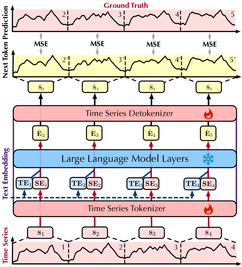
Figure 2: Overview of AutoTimes. To fully leverage the inherent token transition of LLMs, AutoTimes establishes the tokenization of time series and utilizes textual covariates in segments, accomplished by the consistent training task of the next token prediction.

Token-wise prompting

Since the textual covariates of time series are generally recorded at each timestamp, sequence-wise prompting in previous works (Jin et al., 2023; Liu et al., 2023b) may lead to excessive length of language prompts, impeding large language models from paying attention to series tokens and inducing time-consuming forwarding. Considering the sequential formulation shared by language and time series, we propose to aggregate textual covariates within the corresponding time series segment:

$$\mathbf{sp}_{i}=\operatorname{Prompt}(\{\mathbf{a}_{(i-1)S+1},\dots,\mathbf{a}_{iS}\}),$$ (4)

and then use the sequential series-text pairs $\{(\mathbf{s}_{i},\mathbf{sp}_{i})\}$ to obtain the embeddings of the blended tokens and enjoy the inherent transition of large language models. The prompting template $\operatorname{Prompt}(\cdot)$ is demonstrated in Figure 3, which is by default composed of the starting and ending timestamps. We observe that the simple prompt can boost the forecasting performance in Section 4.4, aiding the LLM to be aware of the seasonal patterns and align different variates under Channel Independence. To obtain one embedding that perceives the token-wise prompt of variable length, we add a special token <EOS> at the end of the prompt. Since all the previous tokens are visible to the special token throughout the causal attention, we select the embedding of <EOS> as $\mathbf{TE}_{i}\in\mathbb{R}^{D}$ integrating textual covariates within a segment:

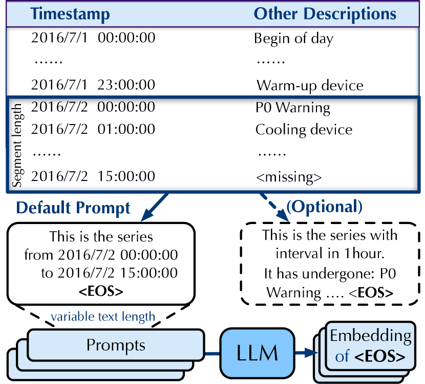
Figure 3: Prompt template of timestamps. We utilize the last token embedding to aggregate the prompt with different text lengths.

$$\mathbf{TE}_{i}=\operatorname{SelectLast}\big{(}\operatorname{LLM}(\{\mathbf{sp}_{i};\verb|<EOS>|\})\big{)}.$$ (5)

Notably, the text embedding $\mathbf{TE}_{i}$ can be precomputed by LLMs and composable if optional descriptions are provided. Benefiting from the homeomorphic alignment of time series segments, the text embedding $\mathbf{TE}_{i}$ can be accordingly integrated with the series embedding $\mathbf{SE}_{i}$. The embedding $\mathbf{E}_{i}\in\mathbb{R}^{D}$ is the sum of text and series embeddings, where $\mathbf{TE}_{i}$ serves as the position embedding of LLMs with enriched periodic and sampling information of time series:

$$\mathbf{E}_{i}=\mathbf{SE}_{i}+\mathbf{TE}_{i}.$$ (6)

3.2 Next Token Prediction

Table 2: Long-term forecasting results averaged from four prediction lengths $S\in\{96,192,336,720\}$. The context length of our proposed method is set as $672$ for all prediction lengths. Deep forecasters are respectively trained on different prediction lengths and the lookback length is also searched from $\{96,192,336,512,672,720\}$ to report the best results. Results of other LLM-based forecasters are reported based on their original paper and “-” indicates not reported. Full results can be found in Table 9.

	LLMs for Time Series Method										Deep Forecaster
Method	AutoTimes		TimeLLM		LLM4TS		FPT		UniTime		iTrans.		DLinear		PatchTST		TimesNet
	(Ours)		(2023)		(2023)		(2023)		(2023b)		(2023c)		(2023)		(2022)		(2022)
Metric	MSE	MAE	MSE	MAE	MSE	MAE	MSE	MAE	MSE	MAE	MSE	MAE	MSE	MAE	MSE	MAE	MSE	MAE
ETTh1	0.389	0.422	0.408	0.423	0.404	0.418	0.427	0.426	0.442	0.448	0.438	0.450	0.423	0.437	0.413	0.431	0.458	0.450
ECL	0.159	0.253	0.159	0.253	0.159	0.253	0.167	0.263	0.216	0.305	0.161	0.256	0.177	0.274	0.159	0.253	0.192	0.295
Traffic	0.374	0.264	0.388	0.264	0.401	0.273	0.414	0.294	-	-	0.379	0.272	0.434	0.295	0.391	0.264	0.620	0.336
Weather	0.235	0.273	0.225	0.257	0.223	0.260	0.237	0.270	0.253	0.276	0.238	0.272	0.240	0.300	0.226	0.264	0.259	0.287
Solar.	0.197	0.242	-	-	-	-	-	-	-	-	0.202	0.269	0.217	0.278	0.189	0.257	0.200	0.268

Since prevalent LLMs (Brown et al., 2020; Touvron et al., 2023) are endowed with the capability of autoregressively predicting the target token $\mathbf{s}_{i}$ based on the preceding tokens $\mathbf{s}_{<i}$, we repurpose them as forecasters and accomplish predictions in fully consistent approaches. Given the token number of $N$, where the time series of the context length $NS$ is tokenized and embedded into $N$ token embeddings $\{\mathbf{E}_{1},\dots,\mathbf{E}_{N}\}$, the aim is to independently predict the next tokens $\{\hat{s}_{2},\dots,\hat{s}_{N+1}\}$ by the LLM. To leverage the learned language modeling transition learned during pre-training, we feed the embeddings while keeping the LLM frozen:

$$\{\hat{\mathbf{E}}_{2},\dots,\hat{\mathbf{E}}_{N+1}\}=\operatorname{LLMLayers}(\{\mathbf{E}_{1},\dots,\mathbf{E}_{N}\}).$$ (7)

$\operatorname{SeriesDetokenizer}(\cdot):\mathbb{R}^{D}\mapsto\mathbb{R}^{S}$ is established to project each obtained embedding back to the time series segment as

$$\hat{\mathbf{s}}_{i}=\operatorname{SeriesDetokenizer}(\hat{\mathbf{E}}_{i}).$$ (8)

Finally, each predicted segment is independently supervised by the ground truth to optimize the parameters of the newly established time series tokenizer and detokenizer, which are both implemented by multi-layer perceptrons:

$$\mathcal{L}_{\text{MSE}}=\frac{1}{NS}\sum||\mathbf{s}_{i}-\hat{\mathbf{s}}_{i}||_{2}^{2},\ i\in\{2,\dots,N+1\}.$$ (9)

By adopting the same generative objective, the repurposed forecaster exhibits similar properties as LLMs such as flexible context lengths empowered by RoPE (Su et al., 2024) as well as the autoregressive style of token generation:

$$\hat{\mathbf{s}}_{i}=\operatorname{LLMForecaster}(\mathbf{s}_{<i}),\ i\in\{1,\dots,\frac{F}{S}\},$$ (10)

which enables one model to handle variable lookback and forecast horizons, instead of respectively training encoder-only forecasters for each horizon. Besides, with the establishment of time series tokenization and full reutilization of LLM parameters, AutoTimes reserves advance capabilities of LLMs, which will be validated in Sections 4.2 and 4.3.

4 Experiments

We thoroughly evaluate the AutoTimes method on various time series forecasting benchmarks, including the forecasting performance of adapted large language models and further validation on zero-shot generability, in-context learning, and multimodal utilization migrated from LLMs. Additional analyses are provided to verify the method generality and benefit of scaling up the repurposed large language model.

Table 3: Short-term forecasting results averaged from all subsets of M4 (Makridakis et al., 2020). The context length of AutoTimes and the lookback length of other methods are set as $2F$, where $F$ is the forecast length of each subset. Full results is provided in Table 10.

Method		AutoTimes	TimeLLM	FPT	Koopa	NHiTS	DLinear	PatchTST	MICN	TimesNet	FiLM	NBEATS
		(Ours)	(2023)	(2023)	(2023d)	(2023)	(2023)	(2022)	(2022a)	(2022)	(2022a)	(2019)
Average	SMAPE	11.831	11.983	11.991	11.863	11.960	12.418	13.022	13.023	11.930	12.489	11.910
	MASE	1.585	1.595	1.600	1.595	1.606	1.656	1.814	1.836	1.597	1.690	1.613
	OWA	0.850	0.859	0.861	0.858	0.861	0.891	0.954	0.960	0.867	0.902	0.862

Table 4: Zero-shot forecasting results in averaged SMAPE. M4 $\to$ M3 means training the model on the datasets of M4 and then evaluating on M3, and vice versa. Results of compared methods are reported from Jin et al. (2023). Full results can be found in Table 12.

Method	AutoTimes	FPT	DLinear	PatchTST	TimesNet	NSformer	FEDformer	Informer	Reformer
Scenario	(Ours)	(2023)	(2023)	(2022)	(2022)	(2022)	(2022b)	(2021)	(2020)
M4$\ \to\$M3	12.75	13.06	14.03	13.06	14.17	15.29	13.53	15.82	13.37
M3$\ \to\$M4	13.036	13.125	15.337	13.228	14.553	14.327	15.047	19.047	14.092

4.1 Time Series Forecasting

Benchmarks

For long-term time series forecasting, we extensively include real-world datasets in our experiments, including ETTh1, ECL, Traffic, Weather, and Solar-Energy used by iTransformer (Liu et al., 2023c). For short-term forecasting, we evaluate the performance on well-acknowledged M4 competition (Makridakis et al., 2020). Detailed dataset descriptions are provided in Appendix A.

Baselines

We extensively compare the proposed method with the state-of-the-art forecasting approaches, including the most recent LLM4TS methods: TimeLLM (2023), LLM4TS (2023), FPT (2023), and UniTime (2023b); the well-acknowledged deep forecasters: iTransformer (2023c), DLinear (2023), PatchTST (2022), and TimesNet (2022). For the challenging short-term forecasting scenario, we further include competitive forecasters: Koopa (2023d), N-HiTS (2023) and N-BEATS (2019). All the baselines are reported based on the original paper or official code. We repurpose LLaMA-7B (Touvron et al., 2023) as our base. The detailed code implementation is provided in Appendix B.

Results

The average results are presented in Table 2–3, with the best results in bold and the second best underlined. AutoTimes demonstrates competitive performance in long-term scenarios, surpassing state-of-the-art LLM4TS methods and deep forecasters in $60\%$ forecasting settings without tuning the lookback length, and consistently outperforms all counterparts in short-term forecasting in Table 3. Notably, AutoTimes is the sole method that trains one single model to cope with variable forecast lengths by autoregressive generation, whereas all other forecasters necessitate training respectively on different lengths and work as a settled function on the rigid forecast length. The costly time and resource consumption of training forecasters and inflexibility on series length can serve as a primary obstacle in real-world deployment.

Generally, the prevailing state-of-the-art deep forecasters are endowed with the encoder-only architecture. To cope with the demand for prolonged prediction, they require rolling forecasting, which involves appending predicted series as the lookback and repeatedly forwarding. Nonetheless, this approach can suffer from error accumulation and the fixed context length of trained models. By contrast, our autoregressive forecaster has been supervisedly trained on each context length during the next token prediction as Equation 9. Furthermore, our repurposed model is developed to be more robust due to the inherent adaptiveness of context length in LLMs. To present a clear comparison, we provide additional results in Table 5 that evaluate our forecaster with other deep models by rolling forecasting under the unified lookback length of $672$, further validating the superior performance of AutoTimes.

Table 5: Averaged results of one model for all prediction lengths. AutoTimes-repurposed LLMs cope with the scenario by autoregressive generation while other deep forecasters necessitate rolling forecasting. Full results can be found in Table 11.

Method	Ours	iTrans.	DLin.	Patch.	Times.
ECL	0.159	0.164	0.165	0.169	0.201
ETTh1	0.389	0.421	0.426	0.409	0.495
Traffic	0.374	0.384	0.423	0.391	0.602
Weather	0.235	0.266	0.239	0.226	0.264
Solar.	0.197	0.213	0.222	0.213	0.202

4.2 Zero-shot Forecasting

Setups

Large language models have exhibited remarkable zero-shot generalization capability (Brown et al., 2020), which can be extremely benefitial for data-scarce applications. To ascertain whether our repurposed LLM forecaster inherits the ability for the common and realistic forecasting scenario, where no training sample is available on the target domain, we evaluate the performance under zero-shot forecasting. Specifically, we follow the benchmark adopted by Zhou et al. (2023), where the forecaster is first trained on a source domain and then directly evaluated on the unseen target domain. We adopt well-acknowledged M3 and M4 competitions, which both contain profused temporal variation patterns but follow different distributions, to set up the challenging zero-shot evaluation. We compare AutoTimes with the aforementioned deep forecasters and FPT as the LLM4TS method since only FPT has demonstrated zero-shot generalization on this benchmark.

Results

The comprehensive results of zero-shot forecasting are listed in Table 4. AutoTimes demonstrates superior performance compared to the previous deep forecasters and FPT in both M4 $\to$ M3 and M3 $\to$ M4 scenarios. It can be observed that LLM4TS methods generally achieve better performance on this task with the enhanced model capacity, resulting in a 15% SMAPE reduction compared with the efficient forecaster DLinear. Based on the same Transformer backbone, LLM4TS methods still achieve better results compared to PatchTST due to the transferable knowledge pre-trained from large corpora of sequences. It confirms the promising advantages of utilizing LLMs for time series forecasting. Furthermore, AutoTimes maintains consistency in training, inference, and parameters of LLMs, thereby outperforming the FPT even without costly fine-tuning.

4.3 In-context Forecasting

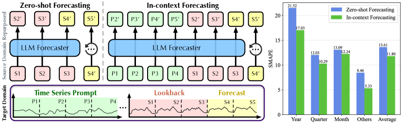
Figure 4: Demonstration of in-context forecasting and the quantitative results on M3. We uniformly select the first time series from the target domain as the prompt and concatenate with the lookback to forecast autoregressively. AutoTimes repurposes LLMs with an enlarged context length of $3F$ to place the additional time series prompt. Supplementary showcases are provided in Appendix D.

Setups

Large language models are capable of generating expected outputs based on provided instructions or task demonstrations in natural language without gradient updating, known as the in-context learning capability (Radford et al., 2021). It is one of the fundamental capabilities for language-based Artificial General Intelligence (AGI). And it is also prevalent in the forecasting scenario, where expert guidance for predicting the series is available to enhance the forecasting. Motivated by this, we investigate whether an LLM-repurposed forecaster can utilize the instructions or demonstrations of time series. Consequently, we propose in-context forecasting in this paper. Based on the zero-shot forecasting scenario, we uniformly select time series from the target domain as the demonstration and adopt it as the prompt. The composed “time series sentence” is fed into our forecaster for the prediction of the lookback window. Prior to this work, none of the LLM4TS methods explored the potential due to the modality misalignment of the tokens in sequence-wise prompting as shown in Figure 1(b).

Results

We provide both demonstration and quantitative evaluation of in-context forecasting in Figure 4. Benefiting from the time series prompt from the target domain, AutoTimes revitalizes the in-context learning capability of LLMs surprisingly, leading to consistent promotions on all M3 subsets and the averaged $13.3\%$ SMAPE reduction compared with zero-shot forecasting. In contrast to previous LLM4TS methods that rely on prompting with text tokens, which may result in potential token disparities and excessive context length, LLMs repurposed by AutoTimes can be instructed by time series natively with established series tokenization. Due to the constraints of training resources, we are only able to repurpose LLaMA-7B currently, which can be still too small to exhibit remarkable in-context learning ability compared with its larger variates (Touvron et al., 2023). However, the results present a promising direction to develop the foundation model of time series on larger LLMs, where scenario-specific instructions can be interactively utilized for more accurate prediction.

4.4 Method Analysis

In this section, we conduct extensive analyses of AutoTimes, with a focus on the applicability of the proposed method and further utilization of booming large language models.

Method generality

While previous works only apply their method on the specific large language model, AutoTimes can be easily applied to various kinds of LLMs since the prevalent LLMs are generally trained autoregressively with the decoder-only architecture (Zhao et al., 2023). We evaluate AutoTimes on several alternative LLMs, including GPT-2 (Radford et al., 2019), OPT (Zhang et al., 2022), and LLaMA (Touvron et al., 2023). The averaged results are listed in Table 6, revealing the notable generality of AutoTimes. More importantly, the repurposed forecaster demonstrates better performance with the increase of parameters, which further validates the scaling law (Kaplan et al., 2020) in LLM-repurposed forecasters.

Table 6: Results of alternative LLMs. The averaged results of prediction lengths are reported. Full results can be found in Table 13.

LLM	GPT-2 (124M)		OPT-2.7B		LLaMA-7B
Metric	MSE	MAE	MSE	MAE	MSE	MAE
ECL	0.173	0.266	0.164	0.258	0.159	0.253
ETTh1	0.397	0.425	0.394	0.424	0.391	0.423
Traffic	0.406	0.276	0.394	0.269	0.374	0.264
Weather	0.242	0.278	0.243	0.277	0.235	0.273

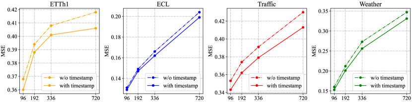
Figure 5: Ablation on token-wise prompting that utilizes timestamps as the instruction under different forecast lengths.

Method efficiency

We thoroughly evaluate the effectiveness of each repurposed LLM from three perspectives: forecasting error, training speed, and parameters, as depicted in Figure 6. In addition to validating the model scalability, we observe that LLaMA-7B serves as the promising choice for LLM-based forecasters, which achieves the consistent best performance. OPT-1.3B also exhibits good parameter efficiency on the evaluated datasets.

Table 7: Trained parameters by AutoTimes in LLaMA-7B.

Dataset	ETTh1	ECL	Solar.	Traffic	Weather
Params.	0.79M	8.59M	8.59M	8.59M	4.30M
Ratio	0.01%	0.12%	0.12%	0.12%	0.06%

Notably, despite LLM having a substantial amount of parameters, AutoTimes requires only minimal parameters for training. It is due to the freezing of Transformer layers, with the introduction of a pair of multi-layer perceptrons for time series tokenization as the LLM plugin. We quantified the number of parameters trained to achieve the performance listed in Table 2. AutoTimes introduces a considerably small amount of parameters, with the ratio to the large language models being comparable to that of LoRA (Hu et al., 2021), as adopted in previous LLM4TS methods ($0.12\%$ under the LoRA rank of $16$). Moreover, they still need to learn additional trainable parameters of time series embedding and projector. By contrast, the results confirm the effectiveness of reutilizing the inherent token transition of AutoTimes.

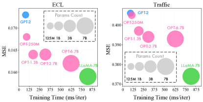
Figure 6: Efficiency comparison on ECL and Traffic, reported with the configuration of Table 6 and the same batch size of $512$.

Variable lookback length

Benefiting from Rotary Position Embedding  (Su et al., 2024) of LLMs, our forecaster has the flexibility to accommodate time series of different lookback lengths without re-training. Moreover, several works have observed that the performance does not necessarily improve with the increasing of lookback length (Zeng et al., 2023). As language models can generally give more accurate answers with a longer context, we evaluate a single repurposed forecaster by gradually increasing the lookback length. As shown in Figure 7, the performance is generally improving with the more available lookback observations, leading to an averaged $9.3\%$ promotion from $192$ to $672$.

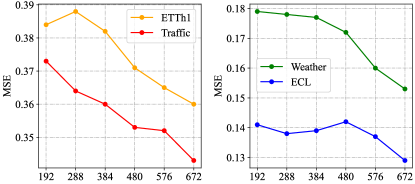
Figure 7: Performance of one forecaster with prolonged lookback.

Utilizing timestamps

We conduct the ablation on the proposed token-wise prompting by integrating timestamps, the most common textual instructions in the real world. As depicted in Figure 5, the forecasting performance is consistently promoted across all datasets and forecasting lengths. The improvement can be attributed to auxiliary periodicity and frequency information, which is significantly beneficial for long-term forecasting. It is also notable that the texts are integrated with time series at the token level of sequence, enabling our method applicable to various forecast scenarios where the instructive texts such as news and logs are simultaneously recorded by time.

5 Conclusion

Based on the commonality in modality and task objectives, large language models naturally serve as foundation models of time series. Different from previous methods that leverage LLMs with inconsistency in training, inference, and parameters, our approach establishes similar tokenization of time series by the next token prediction, adopts the same autoregressive generation for inference, and freezes the blocks of LLMs to fully reutilize the inherent token transition. Experimentally, our repurposed forecasters demonstrate competitive results with existing benchmarks and have shown proficiency in handling variable series lengths. Further analysis reveals that our approach effectively reserves advanced capabilities such as zero-shot generalization and in-context learning, making it feasible to utilize both instructive times series and timestamps. In the future, we will further delve into tokenization and adapt larger language models.

Appendix A Dataset Descriptions

We evaluate the performance of the proposed AutoTimes through experiments conducted on seven real-world datasets. These datasets encompass various domains: (1) ETT (Zhou et al., 2021) spans from July 2016 to July 2018 and consists of seven factors related to electricity transformers. It comprises four subsets: ETTh1 and ETTh2 with hourly recordings, and ETTm1 and ETTm2 with recordings every 15 minutes. (2) Weather  (Wu et al., 2021) encompasses 21 meteorological factors collected every 10 minutes in 2020 from the Weather Station of the Max Planck Biogeochemistry Institute. (3) ECL (Wu et al., 2021) captures hourly electricity consumption data from 321 clients. (4) Traffic  (Wu et al., 2021) gathers hourly road occupancy rates from 862 sensors on San Francisco Bay area freeways spanning from January 2015 to December 2016. (5) Solar-Energy (Lai et al., 2018) records solar power production from 137 PV plants in 2006, sampled every 10 minutes. (6) M4 is a comprehensive dataset encompassing various time series across different fields such as business, finance, and economics. (7) M3, albeit smaller than M4, also contains diverse time series from various domains and frequencies.

We follow the same data processing and train-validation-test set split protocol used in TimesNet (Wu et al., 2021), where the train, validation, and test datasets are strictly divided according to chronological order to ensure no data leakage issues. As for the forecasting settings, we fix the length of the lookback series as 672 in ETT, ECL, Traffic, Weather, and Solar-Energy, and the prediction length varies in {96, 192, 336, 720}. The details of datasets are provided in Table 8.

Table 8: Detailed dataset descriptions. Dim denotes the variate number of each dataset. Dataset Size denotes the total number of time points in (Train, Validation, Test) split respectively. Prediction Length denotes the future time points to be predicted and four prediction settings are included in each dataset. Frequency denotes the sampling interval of time points.

Dataset	Dim	Prediction Length	Dataset Size	Frequency	Information
ETTh1	7	{96, 192, 336, 720}	(8545, 2881, 2881)	Hourly	Electricity
Weather	21	{96, 192, 336, 720}	(36792, 5271, 10540)	10min	Weather
ECL	321	{96, 192, 336, 720}	(18317, 2633, 5261)	Hourly	Electricity
Traffic	862	{96, 192, 336, 720}	(12185, 1757, 3509)	Hourly	Transportation
Solar-Energy	137	{96, 192, 336, 720}	(36601, 5161, 10417)	10min	Energy
M4-Yearly	1	6	(23000, 0, 23000)	Yearly	Demographic
M4-Quarterly	1	8	(24000, 0, 24000)	Quarterly	Finance
M4-Monthly	1	18	(48000, 0, 48000)	Monthly	Industry
M4-Weekly	1	13	(359, 0, 359)	Weekly	Macro
M4-Daily	1	14	(4227, 0, 4227)	Daily	Micro
M4-Hourly	1	48	(414, 0, 414)	Hourly	Other
M3-Yearly	1	6	(645, 0, 645)	Yearly	Demographic
M3-Quarterly	1	8	(756, 0, 756)	Quarterly	Finance
M3-Monthly	1	18	(1428, 0, 1428)	Monthly	Industry
M3-Others	1	8	(174, 0, 174)	Weekly	Macro

Appendix B Implementation Details

AutoTimes processes timestamps in textual form rather than numerical encoding, potentially enabling handling other textual data such as news or logs. We utilize LLM to obtain embedding for the special token <EOS> to capture embedding for the entire sentence. Pseudo-code for this process is depicted in Algorithm 1. It’s worth noting that in the context of multivariate time series forecasting, timestamps are shared across variates. Thus, timestamps can implicitly express relationships between variates even with channel independence. Further, assuming there are $C$ variates since the number of timestamps is $\frac{1}{C}$ of the total time point count, its embedding can be efficiently precomputed by large language models.

After obtaining embedding for the timestamps, we repurpose LLM for time series forecasting using Algorithm 2. At this stage, only the parameters of $\operatorname{SeriesTokenizer}$ and $\operatorname{SeriesDetokenizer}$ are updated, while the parameters of LLM remain entirely frozen. During inference, AutoTimes utilizes the last token generated as its prediction and then employs this output to create subsequent predictions autoregressively. This approach enables AutoTimes to predict sequences of variable lengths with just one model dynamically. Such capability is particularly crucial in real-world application scenarios. The pseudo-code in Algorithm 3-4 illustrates this process.

All the experiments are conducted using PyTorch (Paszke et al., 2019) on NVIDIA A100-40G GPUs. We employ Adam (Kingma & Ba, 2014) with an initial learning rate in {$10^{-3},5\times 10^{-4},10^{-4}$} and MSE loss for model optimization. Additionally, we transform the multivariate data into univariate data by treating each feature of the sequence as an individual time series. The batch size is chosen from {256, 1024, 2048}, and we limit the number of training epochs to 10. As for $\operatorname{SeriesTokenizer}$ and $\operatorname{SeriesDetokenizer}$, we use either linear layers or multi-layer perceptrons. All experiments are based on the benchmark provided by the TimesNet (Wu et al., 2021) repository, which is fairly built on the configurations provided by each model’s original paper or official code.

Algorithm 1 AutoTimes - Generate Text Embedding

0:  Textual covariates $\mathbf{a}_{(i-1)S+1:iS}$ $\triangleright$ $i$-th token of length $S$

1:  $\mathbf{sp}_{i}=\operatorname{Prompt}(\{\mathbf{a}_{(i-1)S+1},\dots,\mathbf{a}_{iS}\})$ $\triangleright$ Dimensionality of LLM hidden states $D$

2:  $\mathbf{TE}_{i}=\operatorname{SelectLast}\big{(}\operatorname{LLM}(\{\mathbf{sp};\verb|<EOS>|\})\big{)}$ $\triangleright$ $\mathbf{TE}_{i}\in\mathbb{R}^{D}$

3:  $\textbf{Return}\ \mathbf{TE}_{i}$ $\triangleright$ Return textual embedding of $i$-th token

Algorithm 2 AutoTimes - Repurpose LLM

0:  Input time series $\{x_{1},\dots,x_{(N+1)\times S}\}$; text embeddings $\{\mathbf{TE}_{1},\dots,\mathbf{TE}_{N}\}$ $\triangleright$ Token number $N$

1:  $\textbf{for}\ i\ \textbf{in}\ \{1,\dots,N\}\textbf{:}$

2:  $\textbf{{\color[rgb]{1,1,1}for}}\ \mathbf{s}_{i}=\{x_{(i-1)S+1},\dots,x_{iS}\}$ $\triangleright$ $\mathbf{s}_{i}\in\mathbb{R}^{S}$

3:  $\textbf{{\color[rgb]{1,1,1}for}}\ \mathbf{SE}_{i}=\operatorname{SeriesTokenizer}(\mathbf{s}_{i})$ $\triangleright$ $\mathbf{SE}_{i}\in\mathbb{R}^{D}$

4:  $\textbf{{\color[rgb]{1,1,1}for}}\ \mathbf{E}_{i}=\mathbf{SE}_{i}+\mathbf{TE}_{i}$ $\triangleright$ $\mathbf{E}_{i}\in\mathbb{R}^{D}$

5:  $\{\hat{\mathbf{E}}_{2},\dots,\hat{\mathbf{E}}_{N+1}\}=\operatorname{LLMLayers}(\{\mathbf{E}_{1},\dots,\mathbf{E}_{N}\})$ $\triangleright$ $\hat{\mathbf{E}}_{i}\in\mathbb{R}^{D}$

6:  $\textbf{for}\ i\ \textbf{in}\ \{2,\dots,N+1\}\textbf{:}$

7:  $\textbf{{\color[rgb]{1,1,1}for}}\ \hat{\mathbf{s}}_{i}=\operatorname{SeriesDetokenizer}(\hat{\mathbf{E}}_{i})$ $\triangleright$ $\hat{\mathbf{s}}_{i}\in\mathbb{R}^{S}$

8:  $\mathbf{s}_{N+1}=\{x_{NS+1},\dots,x_{NS+S}\}$

9:  $\mathcal{L}_{\text{MSE}}=\frac{1}{NS}\sum||\mathbf{s}_{i}-\hat{\mathbf{s}}_{i}||_{2}^{2},\ i\in\{2,\dots,N+1\}$ $\triangleright$ Objective of the next token prediction

Algorithm 3 AutoTimes - LLM Forecasting

0:  Input time series $\{x_{1},\dots,x_{N_{1}\times S}\}$; text embeddings $\{\mathbf{TE}_{1},\dots,\mathbf{TE}_{N_{1}}\}$ $\triangleright$ Lookback token number $N_{1}\leq N$

1:  $\textbf{for}\ i\ \textbf{in}\ \{1,\dots,N_{1}\}\textbf{:}$

2:  $\textbf{{\color[rgb]{1,1,1}for}}\ \mathbf{s}_{i}=\{x_{(i-1)S+1},\dots,x_{iS}\}$ $\triangleright$ $\mathbf{s}_{i}\in\mathbb{R}^{S}$

3:  $\textbf{{\color[rgb]{1,1,1}for}}\ \mathbf{SE}_{i}=\operatorname{SeriesTokenizer}(\mathbf{s}_{i})$ $\triangleright$ $\mathbf{SE}_{i}\in\mathbb{R}^{D}$

4:  $\textbf{{\color[rgb]{1,1,1}for}}\ \mathbf{E}_{i}=\mathbf{SE}_{i}+\mathbf{TE}_{i}$ $\triangleright$ $\mathbf{E}_{i}\in\mathbb{R}^{D}$

5:  $\{\hat{\mathbf{E}}_{2},\dots,\hat{\mathbf{E}}_{N_{1}+1}\}=\operatorname{LLMLayers}(\{\mathbf{E}_{1},\dots,\mathbf{E}_{N_{1}}\})$ $\triangleright$ $\hat{\mathbf{E}}_{i}\in\mathbb{R}^{D}$

6:  $\textbf{for}\ i\ \textbf{in}\ \{2,\dots,N+1\}\textbf{:}$

7:  $\textbf{{\color[rgb]{1,1,1}for}}\ \hat{\mathbf{s}}_{i}=\operatorname{SeriesDetokenizer}(\hat{\mathbf{E}}_{i})$ $\triangleright$ $\hat{\mathbf{s}}_{i}\in\mathbb{R}^{S}$

8:  Return $\hat{\mathbf{s}}_{N+1}$ $\triangleright$ Return last token $\hat{\mathbf{s}}_{N+1}\in\mathbb{R}^{S}$ as the prediction

Algorithm 4 AutoTimes - Autoregressive Generation

0:  Input time series $\{x_{1},\dots,x_{N_{1}\times S}\}$; text embeddings $\{\mathbf{TE}_{1},\dots,\mathbf{TE}_{N_{2}}\}$ $\triangleright$ Forecast token number $N_{2}-N_{1}$

1:  $\mathbf{x}=\{x_{1},\dots,x_{N_{1}\times S}\}$

2:  prediction = {}

3:  $\textbf{for}\ i\ \textbf{in}\ \{1,\dots,N_{2}-N_{1}\}\textbf{:}$

4:  $\textbf{{\color[rgb]{1,1,1}for}}\ \hat{\mathbf{y}}=\operatorname{LLMForecaster}(\mathbf{x},\mathbf{TE}_{:N_{1}+i-1})$ $\triangleright$ Details in Algorithm 3

5:  $\textbf{{\color[rgb]{1,1,1}for}}\ \mathbf{x}\leftarrow\{\mathbf{x},\hat{\mathbf{y}}\}$ $\triangleright$ Concatenate for the input for next iteration

6:  $\textbf{{\color[rgb]{1,1,1}for}}\ \text{prediction}\leftarrow\{\text{prediction},\hat{\mathbf{y}}\}$ $\triangleright$ Record prediction results

7:  Return prediction $\triangleright$ Return result $\in\mathbb{R}^{(N_{2}-N_{1})\times S}$

Appendix C Full Results

C.1 Time Series Forecasting

We compare the performance of AutoTimes with previous state-of-the-art LLM4TS methods and well-acknowledged deep forecasters. Table 9 presents detailed long-term forecast results on ETTh1, ECL, Traffic, Weather, and Solar-Energy datasets, and Table 10 shows detailed short-term forecast results on M4. It is worth noting that in these experiments, AutoTimes only trains a single model per dataset to forecast all prediction lengths, whereas other methods train a model for each forecast length. Furthermore, Table 11 presents the results of one trained model for all prediction lengths.

Table 9: Full results of the long-term forecasting task. The context length of AutoTimes is fixed as $672$ for all prediction lengths. Deep forecasters are respectively trained on different prediction lengths and the lookback length is also searched from $\{96,192,336,512,672,720\}$ to report the best results. Results of other LLM-based forecasters are reported based on their original paper and “-” indicates not reported.

Method		AutoTimes		TimeLLM		LLM4TS		FPT		UniTime		iTrans.		DLinear		PatchTST		TimesNet
		(Ours)		(2023)		(2023)		(2023)		(2023b)		(2023c)		(2023)		(2022)		(2022)
Metric		MSE	MAE	MSE	MAE	MSE	MAE	MSE	MAE	MSE	MAE	MSE	MAE	MSE	MAE	MSE	MAE	MSE	MAE
ETTh1	96	0.360	0.400	0.362	0.392	0.371	0.394	0.376	0.397	0.397	0.418	0.386	0.405	0.375	0.399	0.370	0.399	0.384	0.402
	192	0.388	0.419	0.398	0.418	0.403	0.412	0.416	0.418	0.434	0.439	0.422	0.439	0.405	0.416	0.413	0.421	0.557	0.436
	336	0.401	0.429	0.430	0.427	0.420	0.422	0.442	0.433	0.468	0.457	0.444	0.457	0.439	0.443	0.422	0.436	0.491	0.469
	720	0.406	0.440	0.442	0.457	0.422	0.444	0.477	0.456	0.469	0.477	0.500	0.498	0.472	0.490	0.447	0.466	0.521	0.500
	Avg	0.389	0.422	0.408	0.423	0.404	0.418	0.427	0.426	0.442	0.448	0.438	0.450	0.423	0.437	0.413	0.431	0.458	0.450
ECL	96	0.129	0.225	0.131	0.224	0.128	0.223	0.139	0.238	0.196	0.287	0.132	0.227	0.153	0.237	0.129	0.222	0.168	0.272
	192	0.147	0.241	0.152	0.241	0.146	0.240	0.153	0.251	0.199	0.291	0.153	0.249	0.152	0.249	0.147	0.240	0.184	0.289
	336	0.162	0.258	0.160	0.248	0.163	0.258	0.169	0.266	0.214	0.305	0.167	0.262	0.169	0.267	0.163	0.259	0.198	0.300
	720	0.199	0.288	0.192	0.298	0.200	0.292	0.206	0.297	0.254	0.335	0.192	0.285	0.233	0.344	0.197	0.290	0.220	0.320
	Avg	0.159	0.253	0.159	0.253	0.159	0.253	0.167	0.263	0.216	0.305	0.161	0.256	0.177	0.274	0.159	0.253	0.192	0.295
Weather	96	0.153	0.203	0.147	0.201	0.147	0.196	0.162	0.212	0.171	0.214	0.163	0.211	0.152	0.237	0.149	0.198	0.172	0.220
	192	0.201	0.250	0.189	0.234	0.191	0.238	0.204	0.248	0.217	0.254	0.205	0.250	0.220	0.282	0.194	0.241	0.219	0.261
	336	0.256	0.293	0.262	0.279	0.241	0.277	0.254	0.286	0.274	0.293	0.254	0.289	0.265	0.319	0.245	0.282	0.280	0.306
	720	0.331	0.345	0.304	0.316	0.313	0.329	0.326	0.337	0.351	0.343	0.329	0.340	0.323	0.362	0.314	0.334	0.365	0.359
	Avg	0.235	0.273	0.225	0.257	0.223	0.260	0.237	0.270	0.253	0.276	0.238	0.272	0.240	0.300	0.226	0.264	0.259	0.287
Traffic	96	0.343	0.248	0.362	0.248	0.372	0.259	0.388	0.282	-	-	0.351	0.257	0.410	0.282	0.360	0.249	0.593	0.321
	192	0.362	0.257	0.374	0.247	0.391	0.265	0.407	0.290	-	-	0.364	0.265	0.423	0.287	0.379	0.256	0.617	0.336
	336	0.379	0.266	0.385	0.271	0.405	0.275	0.412	0.294	-	-	0.382	0.273	0.436	0.296	0.392	0.264	0.629	0.336
	720	0.413	0.284	0.430	0.288	0.437	0.292	0.450	0.312	-	-	0.420	0.292	0.466	0.315	0.432	0.286	0.640	0.350
	Avg	0.374	0.264	0.388	0.264	0.401	0.273	0.414	0.294	-	-	0.379	0.272	0.434	0.295	0.391	0.264	0.620	0.336
Solar-Energy	96	0.171	0.221	-	-	-	-	-	-	-	-	0.187	0.255	0.191	0.256	0.168	0.237	0.178	0.256
	192	0.190	0.236	-	-	-	-	-	-	-	-	0.200	0.270	0.211	0.273	0.187	0.263	0.200	0.268
	336	0.203	0.248	-	-	-	-	-	-	-	-	0.209	0.276	0.228	0.287	0.196	0.260	0.212	0.274
	720	0.222	0.262	-	-	-	-	-	-	-	-	0.213	0.276	0.236	0.295	0.205	0.269	0.211	0.273
	Avg	0.197	0.242	-	-	-	-	-	-	-	-	0.202	0.269	0.217	0.278	0.189	0.257	0.200	0.268

Table 10: Full results of the short-term forecasting task. We follow the same protocol as Liu et al. (2023d).

Method		AutoTimes	TimeLLM	FPT	Koopa	NHiTS	DLinear	PatchTST	MICN	TimesNet	FiLM	NBEATS
		(Ours)	(2023)	(2023)	(2023d)	(2023)	(2023)	(2022)	(2022a)	(2022)	(2022a)	(2019)
Year	SMAPE	13.319	13.419	13.531	13.352	13.371	13.866	13.517	14.532	13.394	14.012	13.466
	MASE	2.993	3.005	3.015	2.997	3.025	3.006	3.031	3.359	3.004	3.071	3.059
	OWA	0.784	0.789	0.793	0.786	0.790	0.802	0.795	0.867	0.787	0.815	0.797
Quarter	SMAPE	10.101	10.110	10.177	10.159	10.454	10.689	10.847	11.395	10.101	10.758	10.074
	MASE	1.182	1.178	1.194	1.189	1.219	1.294	1.315	1.379	1.183	1.306	1.163
	OWA	0.890	0.889	0.897	0.895	0.919	0.957	0.972	1.020	0.890	0.905	0.881
Month	SMAPE	12.710	12.980	12.894	12.730	12.794	13.372	14.584	13.829	12.866	13.377	12.801
	MASE	0.934	0.963	0.956	0.953	0.960	1.014	1.169	1.082	0.964	1.021	0.955
	OWA	0.880	0.903	0.897	0.901	0.895	0.940	1.055	0.988	0.894	0.944	0.893
Others	SMAPE	4.843	4.795	4.940	4.861	4.696	4.894	6.184	6.151	4.982	5.259	5.008
	MASE	3.277	3.178	3.228	3.124	3.130	3.358	4.818	4.263	3.323	3.608	3.443
	OWA	1.026	1.006	1.029	1.004	0.988	1.044	1.140	1.319	1.048	1.122	1.070
Average	SMAPE	11.831	11.983	11.991	11.863	11.960	12.418	13.022	13.023	11.930	12.489	11.910
	MASE	1.585	1.595	1.600	1.595	1.606	1.656	1.814	1.836	1.597	1.690	1.613
	OWA	0.850	0.859	0.861	0.858	0.861	0.891	0.954	0.960	0.867	0.902	0.862

Table 11: Results of one model for all prediction lengths. AutoTimes tackles the scenarios by autoregressive forecasting with a context length of 672 and other deep forecasters adopt rolling forecasting with a unified lookback length of 672 and forecast length of 96.

Method		Autoregressive		Rolling Forecasting
		AutoTimes (Our)		iTrans. (2023c)		DLinear (2023)		PatchTST (2022)		TimesNet (2022)
Metric		MSE	MAE	MSE	MAE	MSE	MAE	MSE	MAE	MSE	MAE
ETTh1	96	0.360	0.400	0.387	0.418	0.369	0.400	0.374	0.401	0.452	0.463
	192	0.388	0.419	0.416	0.437	0.405	0.422	0.405	0.422	0.474	0.477
	336	0.401	0.429	0.434	0.450	0.435	0.445	0.423	0.435	0.493	0.489
	720	0.406	0.440	0.447	0.473	0.493	0.508	0.434	0.460	0.560	0.534
	Avg	0.389	0.422	0.421	0.445	0.426	0.444	0.409	0.430	0.495	0.491
ECL	96	0.129	0.225	0.133	0.229	0.138	0.238	0.132	0.232	0.184	0.288
	192	0.147	0.241	0.151	0.245	0.152	0.251	0.151	0.250	0.192	0.295
	336	0.162	0.258	0.168	0.262	0.167	0.268	0.171	0.272	0.200	0.303
	720	0.199	0.288	0.205	0.294	0.203	0.302	0.222	0.318	0.228	0.325
	Avg	0.159	0.253	0.164	0.258	0.165	0.265	0.169	0.268	0.201	0.303
Weather	96	0.153	0.203	0.174	0.225	0.169	0.229	0.149	0.202	0.169	0.228
	192	0.201	0.250	0.227	0.268	0.211	0.268	0.194	0.245	0.222	0.269
	336	0.256	0.293	0.290	0.309	0.258	0.306	0.244	0.285	0.290	0.310
	720	0.331	0.345	0.374	0.360	0.320	0.362	0.317	0.338	0.376	0.364
	Avg	0.235	0.273	0.266	0.291	0.239	0.291	0.226	0.268	0.264	0.293
Traffic	96	0.343	0.248	0.353	0.259	0.399	0.285	0.359	0.255	0.593	0.315
	192	0.362	0.257	0.373	0.267	0.409	0.290	0.377	0.265	0.596	0.317
	336	0.379	0.266	0.386	0.275	0.422	0.297	0.393	0.276	0.600	0.319
	720	0.413	0.284	0.425	0.296	0.461	0.319	0.436	0.305	0.619	0.335
	Avg	0.374	0.264	0.384	0.274	0.423	0.298	0.391	0.275	0.602	0.322
Solar.	96	0.171	0.221	0.183	0.265	0.193	0.258	0.168	0.237	0.180	0.272
	192	0.190	0.236	0.205	0.283	0.214	0.274	0.189	0.257	0.199	0.286
	336	0.203	0.248	0.224	0.299	0.233	0.291	0.212	0.277	0.220	0.301
	720	0.222	0.262	0.239	0.316	0.246	0.307	0.240	0.305	0.251	0.321
	Avg	0.197	0.242	0.213	0.291	0.222	0.283	0.202	0.269	0.213	0.295

C.2 Zero-shot Forecasting

In zero-shot forecasting, every experiment comprises two separate datasets: the source and target datasets. We use the source dataset to train the model, which then makes predictions on the target dataset without further fine-tuning.

For M4 $\to$ M3, which means training on M4 and testing on M3, we directly utilize the same model in the short-term forecasting experiments reported in Table 10. Considering different subsets’ horizons, for M3 Yearly, M3 Quarterly, and M3 Monthly, we directly employ models trained on corresponding subsets of M4 for testing. As for M3 Others, we test using the model trained on M4 Quarterly to keep the same horizon.

For M3 $\to$ M4, similarly, for M4 Yearly, M4 Quarterly, and M4 Monthly, we directly employ models trained on corresponding subsets of M3 for testing. For the remaining subsets, M4 Weekly, M4 Daily, and M4 Hourly, we perform inference using the model trained on M3 Monthly. Table 12 shows the detailed result.

Table 12: Full results of the zero-shot forecasting task. We follow the same protocol as Zhou et al. (2023). M4 $\to$ M3 means training the model on the datasets of M4 and then directly evaluating the performance on M3, and vice versa. SMAPE is adopted as the metric.

Method		AutoTimes	FPT	DLinear	PatchTST	TimesNet	NSformer	FEDformer	Informer	Reformer
Scenario		(Ours)	(2023)	(2023)	(2022)	(2022)	(2022)	(2022b)	(2021)	(2020)
M4$\ \to\$M3	Year	15.71	16.42	17.43	15.99	18.75	17.05	16.00	19.70	16.03
	Quarter	9.35	10.13	9.74	9.62	12.26	12.56	9.48	13.00	9.76
	Month	14.06	14.10	15.65	14.71	14.01	16.82	15.12	15.91	14.80
	Others	5.79	4.81	6.81	9.44	6.88	8.13	8.94	13.03	7.53
	Average	12.75	13.06	14.03	13.39	14.17	15.29	13.53	15.82	13.37
M3$\ \to\$M4	Year	13.728	13.740	14.193	13.966	15.655	14.988	13.887	18.542	15.652
	Quarter	10.742	10.787	18.856	10.929	11.877	11.686	11.513	16.907	11.051
	Month	14.558	14.630	14.765	14.664	16.165	16.098	18.154	23.454	15.604
	Others	6.259	7.081	9.194	7.087	6.863	6.977	7.529	7.348	7.001
	Average	13.036	13.125	15.337	13.228	14.553	14.327	15.047	19.047	14.092

C.3 Method generality

Mainstream LLMs predominantly adopt the decoder-only architecture, and AutoTimes can utilize any decoder-only LLM. We conduct experiments on various types and sizes of LLMs, including GPT-2 (Radford et al., 2019), multiple sizes of OPT (Zhang et al., 2022), and LLaMA (Touvron et al., 2023). Specific results are shown in Table 13, demonstrating a general trend where performance improves as the model size increases, consistent with the scaling law (Kaplan et al., 2020).

Table 13: Results of alternative LLMs.

LLM		GPT-2 (124M)		OPT-350M		OPT-1.3B		OPT-2.7B		OPT-6.7B		LLaMA-7B
Metric		MSE	MAE	MSE	MAE	MSE	MAE	MSE	MAE	MSE	MAE	MSE	MAE
ECL	96	0.140	0.236	0.136	0.233	0.132	0.228	0.132	0.227	0.130	0.226	0.129	0.225
	192	0.159	0.253	0.154	0.249	0.150	0.245	0.149	0.244	0.148	0.242	0.147	0.241
	336	0.177	0.270	0.171	0.267	0.167	0.262	0.167	0.262	0.165	0.260	0.162	0.258
	720	0.216	0.303	0.211	0.301	0.206	0.296	0.207	0.297	0.204	0.295	0.199	0.288
	Avg	0.173	0.266	0.168	0.263	0.164	0.258	0.164	0.258	0.162	0.256	0.159	0.253
ETTh1	96	0.360	0.397	0.365	0.403	0.357	0.395	0.360	0.398	0.357	0.397	0.360	0.400
	192	0.391	0.419	0.395	0.423	0.389	0.417	0.389	0.419	0.386	0.417	0.388	0.419
	336	0.408	0.432	0.411	0.434	0.408	0.431	0.404	0.430	0.404	0.429	0.401	0.429
	720	0.429	0.452	0.432	0.457	0.430	0.452	0.421	0.447	0.427	0.454	0.406	0.440
	Avg	0.397	0.425	0.401	0.429	0.396	0.424	0.394	0.424	0.394	0.424	0.389	0.423
Traffic	96	0.369	0.257	0.371	0.260	0.361	0.253	0.358	0.251	0.357	0.251	0.343	0.248
	192	0.394	0.268	0.393	0.270	0.383	0.263	0.380	0.261	0.379	0.261	0.362	0.257
	336	0.413	0.278	0.411	0.279	0.402	0.273	0.399	0.271	0.398	0.272	0.379	0.266
	720	0.449	0.299	0.446	0.300	0.440	0.295	0.437	0.293	0.437	0.294	0.413	0.284
	Avg	0.406	0.276	0.405	0.277	0.397	0.271	0.394	0.269	0.393	0.270	0.374	0.264
Weather	96	0.158	0.208	0.157	0.208	0.157	0.207	0.157	0.207	0.159	0.209	0.153	0.203
	192	0.207	0.254	0.205	0.252	0.207	0.253	0.206	0.253	0.208	0.256	0.201	0.250
	336	0.262	0.298	0.261	0.294	0.263	0.296	0.265	0.297	0.268	0.302	0.256	0.293
	720	0.342	0.353	0.335	0.346	0.334	0.347	0.344	0.351	0.354	0.360	0.235	0.273
	Avg	0.242	0.278	0.240	0.275	0.240	0.276	0.243	0.277	0.247	0.282	0.235	0.273

Appendix D Showcases of In-context Forecasting

For in-context forecasting, similar to zero-shot forecasting in Appendix C.2, we train our model using the source dataset and directly evaluate it on the target dataset. In this task, we choose M4 as the source dataset and M3 as the target dataset. It is important to note that the structure of the M3 and M4 datasets differs from typical datasets used for long-term forecasting. They consist of multiple univariate time sequences of different lengths. The final segment of each sequence serves as the test set, while the preceding segments are used for training.

In zero-shot scenarios, we utilize a sequence of length $F$ preceding the test set as input, referred to as the lookback window, where $F$ is the forecast length of each subset. During in-context forecasting, we concatenate the first $2F$ time points length that belong to the same sequence with the lookback window as input. We aim to enhance prediction performance by incorporating contextual information in this manner. Too short sequences are discarded to prevent overlap between the prompt and the lookback window. For a fair comparison, both zero-shot and in-context forecasting performance are reported on the same remaining sequences. Figure 8 provides showcases of zero-shot and in-context forecasting results.

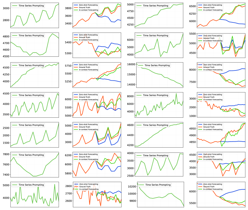
Figure 8: Showcases that compare the forecasting results of zero-shot and in-context forecasting. For in-context forecasting, given a lookback window, we consistently select the first $2F$ time points that belong to the same sequence as the time series prompt.

References

- Alayrac et al. (2022) Alayrac, J.-B., Donahue, J., Luc, P., Miech, A., Barr, I., Hasson, Y., Lenc, K., Mensch, A., Millican, K., Reynolds, M., et al. Flamingo: a visual language model for few-shot learning. Advances in Neural Information Processing Systems, 35:23716–23736, 2022.
- Bengio et al. (2000) Bengio, Y., Ducharme, R., and Vincent, P. A neural probabilistic language model. Advances in neural information processing systems, 13, 2000.
- Bommasani et al. (2021) Bommasani, R., Hudson, D. A., Adeli, E., Altman, R., Arora, S., von Arx, S., Bernstein, M. S., Bohg, J., Bosselut, A., Brunskill, E., et al. On the opportunities and risks of foundation models. arXiv preprint arXiv:2108.07258, 2021.
- Box (2013) Box, G. Box and jenkins: time series analysis, forecasting and control. In A Very British Affair: Six Britons and the Development of Time Series Analysis During the 20th Century, pp. 161–215. Springer, 2013.
- Box et al. (2015) Box, G. E., Jenkins, G. M., Reinsel, G. C., and Ljung, G. M. Time series analysis: forecasting and control. John Wiley & Sons, 2015.
- Brown et al. (2020) Brown, T., Mann, B., Ryder, N., Subbiah, M., Kaplan, J. D., Dhariwal, P., Neelakantan, A., Shyam, P., Sastry, G., Askell, A., et al. Language models are few-shot learners. Advances in neural information processing systems, 33:1877–1901, 2020.
- Cao et al. (2023) Cao, D., Jia, F., Arik, S. O., Pfister, T., Zheng, Y., Ye, W., and Liu, Y. Tempo: Prompt-based generative pre-trained transformer for time series forecasting. arXiv preprint arXiv:2310.04948, 2023.
- Challu et al. (2023) Challu, C., Olivares, K. G., Oreshkin, B. N., Ramirez, F. G., Canseco, M. M., and Dubrawski, A. Nhits: Neural hierarchical interpolation for time series forecasting. In Proceedings of the AAAI Conference on Artificial Intelligence, volume 37, pp. 6989–6997, 2023.
- Chang et al. (2023) Chang, C., Peng, W.-C., and Chen, T.-F. Llm4ts: Two-stage fine-tuning for time-series forecasting with pre-trained llms. arXiv preprint arXiv:2308.08469, 2023.
- Cleveland et al. (1990) Cleveland, R. B., Cleveland, W. S., McRae, J. E., and Terpenning, I. Stl: A seasonal-trend decomposition. J. Off. Stat, 6(1):3–73, 1990.
- Dai et al. (2022) Dai, D., Sun, Y., Dong, L., Hao, Y., Sui, Z., and Wei, F. Why can gpt learn in-context? language models secretly perform gradient descent as meta optimizers. arXiv preprint arXiv:2212.10559, 2022.
- Das et al. (2023) Das, A., Kong, W., Leach, A., Sen, R., and Yu, R. Long-term forecasting with tide: Time-series dense encoder. arXiv preprint arXiv:2304.08424, 2023.
- Dosovitskiy et al. (2020) Dosovitskiy, A., Beyer, L., Kolesnikov, A., Weissenborn, D., Zhai, X., Unterthiner, T., Dehghani, M., Minderer, M., Heigold, G., Gelly, S., et al. An image is worth 16x16 words: Transformers for image recognition at scale. arXiv preprint arXiv:2010.11929, 2020.
- Durbin & Koopman (2012) Durbin, J. and Koopman, S. J. Time series analysis by state space methods, volume 38. OUP Oxford, 2012.
- Gruver et al. (2023) Gruver, N., Finzi, M., Qiu, S., and Wilson, A. G. Large language models are zero-shot time series forecasters. arXiv preprint arXiv:2310.07820, 2023.
- Hoffmann et al. (2022) Hoffmann, J., Borgeaud, S., Mensch, A., Buchatskaya, E., Cai, T., Rutherford, E., Casas, D. d. L., Hendricks, L. A., Welbl, J., Clark, A., et al. Training compute-optimal large language models. arXiv preprint arXiv:2203.15556, 2022.
- Hu et al. (2021) Hu, E. J., Shen, Y., Wallis, P., Allen-Zhu, Z., Li, Y., Wang, S., Wang, L., and Chen, W. Lora: Low-rank adaptation of large language models. arXiv preprint arXiv:2106.09685, 2021.
- Jin et al. (2023) Jin, M., Wang, S., Ma, L., Chu, Z., Zhang, J. Y., Shi, X., Chen, P.-Y., Liang, Y., Li, Y.-F., Pan, S., et al. Time-llm: Time series forecasting by reprogramming large language models. arXiv preprint arXiv:2310.01728, 2023.
- Kaplan et al. (2020) Kaplan, J., McCandlish, S., Henighan, T., Brown, T. B., Chess, B., Child, R., Gray, S., Radford, A., Wu, J., and Amodei, D. Scaling laws for neural language models. arXiv preprint arXiv:2001.08361, 2020.
- Kingma & Ba (2014) Kingma, D. P. and Ba, J. Adam: A method for stochastic optimization. arXiv preprint arXiv:1412.6980, 2014.
- Kitaev et al. (2020) Kitaev, N., Kaiser, Ł., and Levskaya, A. Reformer: The efficient transformer. arXiv preprint arXiv:2001.04451, 2020.
- Lai et al. (2018) Lai, G., Chang, W.-C., Yang, Y., and Liu, H. Modeling long-and short-term temporal patterns with deep neural networks. In The 41st international ACM SIGIR conference on research & development in information retrieval, pp. 95–104, 2018.
- Li et al. (2022) Li, J., Li, D., Xiong, C., and Hoi, S. Blip: Bootstrapping language-image pre-training for unified vision-language understanding and generation. In International Conference on Machine Learning, pp. 12888–12900. PMLR, 2022.
- Liu et al. (2023a) Liu, H., Li, C., Wu, Q., and Lee, Y. J. Visual instruction tuning. arXiv preprint arXiv:2304.08485, 2023a.
- Liu et al. (2023b) Liu, X., Hu, J., Li, Y., Diao, S., Liang, Y., Hooi, B., and Zimmermann, R. Unitime: A language-empowered unified model for cross-domain time series forecasting. arXiv preprint arXiv:2310.09751, 2023b.
- Liu et al. (2022) Liu, Y., Wu, H., Wang, J., and Long, M. Non-stationary transformers: Exploring the stationarity in time series forecasting. Advances in Neural Information Processing Systems, 35:9881–9893, 2022.
- Liu et al. (2023c) Liu, Y., Hu, T., Zhang, H., Wu, H., Wang, S., Ma, L., and Long, M. itransformer: Inverted transformers are effective for time series forecasting. arXiv preprint arXiv:2310.06625, 2023c.
- Liu et al. (2023d) Liu, Y., Li, C., Wang, J., and Long, M. Koopa: Learning non-stationary time series dynamics with koopman predictors. arXiv preprint arXiv:2305.18803, 2023d.
- Makridakis et al. (2020) Makridakis, S., Spiliotis, E., and Assimakopoulos, V. The m4 competition: 100,000 time series and 61 forecasting methods. International Journal of Forecasting, 36(1):54–74, 2020.
- Nie et al. (2022) Nie, Y., Nguyen, N. H., Sinthong, P., and Kalagnanam, J. A time series is worth 64 words: Long-term forecasting with transformers. arXiv preprint arXiv:2211.14730, 2022.
- OpenAI (2023) OpenAI, R. Gpt-4 technical report. arxiv 2303.08774. View in Article, 2:13, 2023.
- Oreshkin et al. (2019) Oreshkin, B. N., Carpov, D., Chapados, N., and Bengio, Y. N-beats: Neural basis expansion analysis for interpretable time series forecasting. arXiv preprint arXiv:1905.10437, 2019.
- Paszke et al. (2019) Paszke, A., Gross, S., Massa, F., Lerer, A., Bradbury, J., Chanan, G., Killeen, T., Lin, Z., Gimelshein, N., Antiga, L., et al. Pytorch: An imperative style, high-performance deep learning library. Advances in neural information processing systems, 32, 2019.
- Radford et al. (2019) Radford, A., Wu, J., Child, R., Luan, D., Amodei, D., Sutskever, I., et al. Language models are unsupervised multitask learners. OpenAI blog, 1(8):9, 2019.
- Radford et al. (2021) Radford, A., Kim, J. W., Hallacy, C., Ramesh, A., Goh, G., Agarwal, S., Sastry, G., Askell, A., Mishkin, P., Clark, J., et al. Learning transferable visual models from natural language supervision. In International conference on machine learning, pp. 8748–8763. PMLR, 2021.
- Su et al. (2024) Su, J., Ahmed, M., Lu, Y., Pan, S., Bo, W., and Liu, Y. Roformer: Enhanced transformer with rotary position embedding. Neurocomputing, 568:127063, 2024.
- Sun et al. (2023) Sun, C., Li, Y., Li, H., and Hong, S. Test: Text prototype aligned embedding to activate llm’s ability for time series. arXiv preprint arXiv:2308.08241, 2023.
- Touvron et al. (2023) Touvron, H., Lavril, T., Izacard, G., Martinet, X., Lachaux, M.-A., Lacroix, T., Rozière, B., Goyal, N., Hambro, E., Azhar, F., et al. Llama: Open and efficient foundation language models. arXiv preprint arXiv:2302.13971, 2023.
- Vaswani et al. (2017) Vaswani, A., Shazeer, N., Parmar, N., Uszkoreit, J., Jones, L., Gomez, A. N., Kaiser, Ł., and Polosukhin, I. Attention is all you need. Advances in neural information processing systems, 30, 2017.
- Wang et al. (2022a) Wang, H., Peng, J., Huang, F., Wang, J., Chen, J., and Xiao, Y. Micn: Multi-scale local and global context modeling for long-term series forecasting. In The Eleventh International Conference on Learning Representations, 2022a.
- Wang et al. (2022b) Wang, T., Roberts, A., Hesslow, D., Le Scao, T., Chung, H. W., Beltagy, I., Launay, J., and Raffel, C. What language model architecture and pretraining objective works best for zero-shot generalization? In International Conference on Machine Learning, pp. 22964–22984. PMLR, 2022b.
- Wei et al. (2022) Wei, J., Tay, Y., Bommasani, R., Raffel, C., Zoph, B., Borgeaud, S., Yogatama, D., Bosma, M., Zhou, D., Metzler, D., et al. Emergent abilities of large language models. arXiv preprint arXiv:2206.07682, 2022.
- Winters (1960) Winters, P. R. Forecasting sales by exponentially weighted moving averages. Management science, 6(3):324–342, 1960.
- Woo et al. (2023) Woo, G., Liu, C., Kumar, A., and Sahoo, D. Pushing the limits of pre-training for time series forecasting in the cloudops domain. arXiv preprint arXiv:2310.05063, 2023.
- Wu et al. (2021) Wu, H., Xu, J., Wang, J., and Long, M. Autoformer: Decomposition transformers with auto-correlation for long-term series forecasting. Advances in Neural Information Processing Systems, 34:22419–22430, 2021.
- Wu et al. (2022) Wu, H., Hu, T., Liu, Y., Zhou, H., Wang, J., and Long, M. Timesnet: Temporal 2d-variation modeling for general time series analysis. arXiv preprint arXiv:2210.02186, 2022.
- Xue & Salim (2023) Xue, H. and Salim, F. D. Promptcast: A new prompt-based learning paradigm for time series forecasting. IEEE Transactions on Knowledge and Data Engineering, 2023.
- Zeng et al. (2023) Zeng, A., Chen, M., Zhang, L., and Xu, Q. Are transformers effective for time series forecasting? In Proceedings of the AAAI conference on artificial intelligence, volume 37, pp. 11121–11128, 2023.
- Zhang et al. (2022) Zhang, S., Roller, S., Goyal, N., Artetxe, M., Chen, M., Chen, S., Dewan, C., Diab, M., Li, X., Lin, X. V., et al. Opt: Open pre-trained transformer language models. arXiv preprint arXiv:2205.01068, 2022.
- Zhao et al. (2023) Zhao, W. X., Zhou, K., Li, J., Tang, T., Wang, X., Hou, Y., Min, Y., Zhang, B., Zhang, J., Dong, Z., et al. A survey of large language models. arXiv preprint arXiv:2303.18223, 2023.
- Zhou et al. (2021) Zhou, H., Zhang, S., Peng, J., Zhang, S., Li, J., Xiong, H., and Zhang, W. Informer: Beyond efficient transformer for long sequence time-series forecasting. In Proceedings of the AAAI conference on artificial intelligence, volume 35, pp. 11106–11115, 2021.
- Zhou et al. (2022a) Zhou, T., Ma, Z., Wen, Q., Sun, L., Yao, T., Yin, W., Jin, R., et al. Film: Frequency improved legendre memory model for long-term time series forecasting. Advances in Neural Information Processing Systems, 35:12677–12690, 2022a.
- Zhou et al. (2022b) Zhou, T., Ma, Z., Wen, Q., Wang, X., Sun, L., and Jin, R. Fedformer: Frequency enhanced decomposed transformer for long-term series forecasting. In International Conference on Machine Learning, pp. 27268–27286. PMLR, 2022b.
- Zhou et al. (2023) Zhou, T., Niu, P., Wang, X., Sun, L., and Jin, R. One fits all: Power general time series analysis by pretrained lm. arXiv preprint arXiv:2302.11939, 2023.
- Zhu et al. (2015) Zhu, Y., Kiros, R., Zemel, R., Salakhutdinov, R., Urtasun, R., Torralba, A., and Fidler, S. Aligning books and movies: Towards story-like visual explanations by watching movies and reading books. In Proceedings of the IEEE international conference on computer vision, pp. 19–27, 2015.