Abstract

We show that in-context learning emerges in transformers in discrete developmental stages, when they are trained on either language modeling or linear regression tasks. We introduce two methods for detecting the milestones that separate these stages, by probing the geometry of the population loss in both parameter space and function space. We study the stages revealed by these new methods using a range of behavioral and structural metrics to establish their validity.

1 Introduction

The configuration space of a cell is high-dimensional, the dynamics governing its development are complex, and no two cells are exactly alike. Nevertheless, cells of the same type develop in the same way: their development can be divided into recognizable stages ending with milestones common to all cells of the same type (Gilbert, 2006). In biology a popular visual metaphor for this dynamic is Waddington’s (1957) developmental landscape, in which milestones correspond to geometric structures that each cell must navigate on its way from a pluripotent form at the top of the landscape to its final functional form at the bottom.

The configuration space of a modern neural network is high-dimensional, the dynamics governing its training are complex, and due to randomness in initialization and the selection of minibatches for training, no two neural networks share exactly the same training trajectory. It is natural to wonder if there is an analogue of the developmental landscape for neural networks. More precisely, we can ask if there is an emergent logic which governs the development of these systems, and whether this logic can be understood in terms of developmental milestones and the stages that separate them. If such milestones exist, we can further ask how they relate to the geometry of the population loss.

We examine these questions for transformers trained in two settings: language modeling, in which a transformer with around 3M parameters is trained on a subset of the Pile (Gao et al., 2020) and linear regression, in which a transformer with around 50k parameters is trained on linear regression tasks following Garg et al. (2022). These settings are chosen because transformers learn to do In-Context Learning (ICL) in both. The emergence of ICL during training (Olsson et al., 2022) is the most conspicuous example of structural development in modern deep learning: a natural starting place for an investigation of the developmental landscape.

We introduce two methods for discovering stages of development in neural network training, both of which are based on analyzing the geometry of the population loss via statistics. The first method is the local learning coefficient (Lau et al., 2023) of Singular Learning Theory (SLT; Watanabe, 2009), which is a measure of the degeneracy of the local geometry of the population loss in parameter space. The second is trajectory PCA, referred to here as essential dynamics (Amadei et al., 1993), which analyzes the geometry of the developmental trajectory in function space. These methods are motivated by the role of geometry in SLT and the connection between milestones in the Waddington landscape and singularities introduced by Thom (1988).

Our methods reveal that, in both the language and linear regression settings, training can be divided into discrete developmental stages according to near plateaus in the local learning coefficient (see Figure 1) and geometric structures in the essential dynamics (see Figure 2).

Our main contribution is to introduce these two methods for discovering stages, and to validate that the stages they discover are genuine by conducting extensive setting-specific analyses to determine the behavioral and structural changes taking place within each stage.

We also initiate the study of forms of the developmental trajectory, which are remarkable geometric objects in function space that we discover occurring at (some) milestones. These forms seem to govern the large scale development of transformers in our two settings. We view the appearance of these structures as evidence in favor of the idea of a simple macroscopic developmental landscape in the sense of Waddington, which governs the microscopic details of the neural network training process.

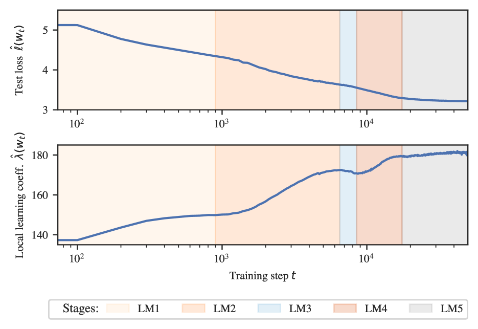
(a) Two-Layer Attention-only Language Transformer.

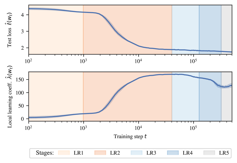
(b) Linear Regression Transformers.

Figure 1: We train transformer models on both (a) natural language data (1 seed) and (b) synthetic in-context regression data (error bars over 5 seeds). In addition to test loss (top row), we track loss landscape degeneracy as quantified by the local learning coefficient (LLC) (bottom row, see Section 3.1). An automated procedure finds plateaus in the LLC, which mark boundaries between distinct developmental stages (ranges of training time indicated with different colors: orange hues for increasing LLC, blue for decreasing). These boundaries are developmental milestones, where certain structures and associated behaviors complete their formation.

2 In-Context Learning

In-Context Learning (ICL), the ability to improve performance on new tasks without changing weights, underlies much of the success of modern transformers Brown et al. (2020). This makes a deeper understanding of ICL necessary to interpreting how and why transformers work. Additionally, ICL is perhaps the clearest example of an “emergent ability” Wei et al. (2022), that appears suddenly as a function of both model depth and training time Olsson et al. (2022). Taken together, this makes ICL uniquely well-motivated as a case study for investigating the learning process of transformers.

Let $f_{w}$ be a transformer with parameters $w$, which takes a context $S_{\leq k}=(t_{1},\ldots,t_{k})$ as input, where $k\leq K$. Let $f_{w}(S_{\leq k})$ be the output logits at token $t_{k}$, and let $n$ be the number of length-$K$ sequences in the training data $\{S^{i}_{K}\}_{i=1}^{n}$.

Given a per-token loss $\ell_{n,k}$ (cross-entropy for language or MSE for linear regression, see Sections 2.1 and 2.2 respectively), the training loss is

$$\ell_{n}(w)=\frac{1}{K}\sum_{k=1}^{K}\ell_{n,k}(w),$$ (1)

with the test loss $\hat{\ell}$ defined analogously on a held-out set of examples.

In general, we say that the trained transformer $f_{w}$ performs ICL if the per-token loss $\ell_{n,k}(w)$ improves consistently with $k$ on an independent test set. More directly, we follow the experimental setup of Olsson et al. (2022) and, dropping the $n$ index, define the ICL score as (see Section C.2.3)

$$\operatorname{ICL}_{k_{1}:k_{2}}(w)=\hat{\ell}_{n,\,k_{1}}(w)-\hat{\ell}_{n,\,k_{2}}(w).$$ (2)

Rather than studying ICL itself, our aim is to study how models develop the ability to perform ICL over the course of training, which we quantify by tracking the ICL score across checkpoints.

2.1 In-Context Learning in Language Models

Following Elhage et al. (2021) and Olsson et al. (2022), we study ICL in autoregressive attention-only (no MLP layers) transformers (details in Section E.1). We consider the standard task of next-token prediction for sequences of tokens taken from a subset of the Pile (Gao et al., 2020; Xie et al., 2023). At the token level, the sample training loss for $k>1$ is the cross-entropy, given by

$$\ell_{n,k}(w)=-\frac{1}{n}\sum_{i=1}^{n}\log\left(\mathrm{softmax}(f_{w}(S_{\leq k}^{i}))[t^{i}_{k+1}]\right).$$ (3)

2.2 In-Context Learning of Linear Functions

Following the framework of Garg et al. (2022), a number of recent works have explored the phenomenon of ICL in the stylized setting of learning simple function classes, such as linear functions. This setting is of interest because we have a precise understanding of theoretically optimal ICL, and because simple transformers are capable of good ICL performance in practice.

In the following we give a standard presentation on ICL of linear functions (full training details in Section E.2). A task is a vector $\task\in\mathbb{R}^{D}$. Given a task $\task$, we generate $x_{i}\in\mathbb{R}^{D},y_{i}\in\mathbb{R}$ iid for $i=1,\ldots,K$ according to the joint distribution $q(x,y|\task)=q(y|x,\task)q(x)$, resulting in the following context,

$$S_{K}=(x_{1},y_{1},\ldots,x_{K-1},y_{K-1},x_{K}),$$

with label $y_{K}$. We limit our study to the setting where $q(y|x,\task)=\mathcal{N}(\task^{T}x,\sigma^{2})$, $q(x)=\mathcal{N}(0,I_{D})$, and task distribution $q(\task)=\mathcal{N}(0,I_{D})$.

Consider a training dataset $\{(\task[i],S_{K}^{i},y_{K}^{i})\}_{i=1}^{n}$ which consists of $n$ iid samples drawn from $q(y|x,\task)q(x)q(\task)$. Upon running a context through the transformer, we obtain a prediction $\hat{y}_{k}^{i}=f_{w}(S_{\leq k}^{i})$ for each subsequence $S_{\leq k}^{i}$, which leads to the per-token training loss

$$\ell_{n,k}(w)=\frac{1}{n}\sum_{i=1}^{n}(\hat{y}^{i}_{k}-y_{k}^{i})^{2}.$$ (4)

3 Methodology

It might seem hopeless to extract geometrical information about a high-dimensional dynamical system like neural network training. But this is not so. It is well-understood that the local geometry of a potential governing a gradient system can have global effects; this has been the basis of deep connections between geometry and topology over the last century (Freed, 2021). In SLT we have a similar principle: the local geometry of the log likelihood has a strong influence on statistical observables, and therefore information about this geometry may be learned from samples.

We use two probes of the geometry of the population loss to study development: the Local Learning Coefficient (LLC) and Essential Dynamics (ED). These indicators are applied to snapshots gathered during training to identify milestones that separate developmental stages. Once identified, we perform a targeted analysis of associated behavioral changes, meaning changes in the input-output behavior of the neural network, and structural changes, meaning changes in the way that the neural network computes internally.

3.1 The Local Learning Coefficient

In Bayesian statistics given a model $p$, true distribution $q$, and parameter $w^{*}$, the Local Learning Coefficient (LLC), denoted $\lambda(w^{*})$, is a positive scalar which measures the degeneracy of the geometry of the population log likelihood function $L$ near $w^{*}$. The more degenerate the geometry, the closer to zero the LLC will be. The LLC is also a measure of model complexity: the larger the LLC, the more complex the model parametrized by $w^{*}$. The learning coefficient and its connection to geometry was introduced by Watanabe (2009) and the local setting was studied by Lau et al. (2023).

Conditions guaranteeing the existence and well-definedness of the theoretical LLC can be found in Lau et al. (2023). For our purposes here, it suffices to explain the LLC estimator proposed there.

The original LLC estimator requires the specification of a log likelihood over iid data, to which we can associate an empirical $L_{n}(w)=-\frac{1}{n}\sum_{i=1}^{n}\log p(z_{i}|w)$ and a population $L(w)=-E_{z}\log p(z|w)$. The LLC estimate $\hat{\lambda}({w^{*}})$, where ${w^{*}}$ is a local minimum of $L(w)$, is

$$\hat{\lambda}({w^{*}})=n\beta\left[\mathbb{E}_{w|{w^{*}},\gamma}^{\beta}[L_{n}(w)]-L_{n}({w^{*}})\right],$$

with $\beta=1/\log n$. The expectation is with respect to a tempered posterior distribution localized at ${w^{*}}$, i.e.,

$$\mathbb{E}_{w|{w^{*}},\gamma}^{\beta}[f(w)]=\int f(w)p(w;{w^{*}},\beta,\gamma,z_{1:n})dw$$

where

$$p(w;{w^{*}},\beta,\gamma,z_{1:n})\propto\exp\{-n\beta L_{n}(w)-\gamma||w-{w^{*}}||^{2}_{2}\}.$$

In this work, we generalize the usage of the original LLC estimator from likelihood-based to loss-based. Given an average empirical loss $\ell_{n}(w)$ over model parameters $w$, the generalized LLC estimate $\hat{\lambda}({w^{*}})$, where ${w^{*}}$ is a local minimum of the corresponding population loss $\ell(w)$, is

$$\hat{\lambda}({w^{*}})=n\beta\left[\mathbb{E}_{w|{w^{*}},\gamma}^{\beta}[\ell_{n}(w)]-\ell_{n}({w^{*}})\right],$$ (5)

where now the expectation is with respect to the loss-based posterior (also known as a Gibbs posterior) given by

$$p(w;{w^{*}},\beta,\gamma,z_{1:n})\propto\exp\left\{-n\beta\ell_{n}(w)-\frac{\gamma}{2}||w-{w^{*}}||^{2}_{2}\right\}.$$ (6)

where $\beta$ is an inverse temperature which controls the contribution of the loss, $\gamma$ is the localization strength which controls proximity to ${w^{*}}$.

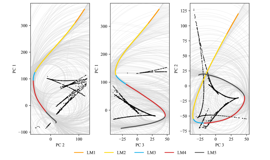
(a) Two-Layer Attention-only Language Transformer.

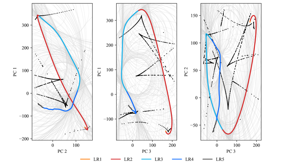
(b) Linear Regression Transformers.

Figure 2: The training trajectory in a subspace of function space projected onto its top three principal components and smoothed, with osculating circles (gray). The evolute, the set of centers of osculating circles, is shown in black. Accentuated families of osculating circles correspond to cusps in the evolute. The corresponding point on the curve (where the evolute “points”) is called a vertex. If a cusp singularity or vertex occurs at the same time in all plots, we infer the presence of a form. (a) Forms $1,2$ at the LM2–LM3, LM4–LM5 boundaries, respectively. Explained variances $0.56,0.15,0.07$. (b) Forms $1$, $2$, and $3$ respectively at the LR1–LR2, LR2–LR3, LR3–LR4 boundaries. Explained variances $0.65,0.08,0.05$.

There are various important factors in the implementation of LLC estimation. The most important is the sampling method used to approximate the expectation over the localized posterior in 6. We employ SGLD and detail diagnostics for tuning its hyperparameters in Appendices A and E.3.

3.2 Essential Dynamics

The parameter space of modern neural networks is usually high-dimensional. Therefore, to study the development of structure in neural networks over training, it is natural to apply methods of dimensionality reduction. Similar problems of data analysis are faced in many sciences, and the application of PCA to trajectories of systems undergoing development is common in neuroscience (Briggman et al., 2005; Cunningham & Yu, 2014) and molecular dynamics (Amadei et al., 1993; Meyer et al., 2006; Hayward & De Groot, 2008).

Following the terminology in molecular dynamics we refer our version of this method as Essential Dynamics (ED).

Suppose a stochastic process $a_{t}\in\mathbb{R}^{s}$ is a function of the weight parameter $w_{t}$ (and possibly other random variables) at a step $t$ in training. Let $A_{t_{1}},\dots,A_{t_{T}}$ be samples from the stochastic process at steps $t_{1},\dots,t_{T}$. Let $A$ denote the $s\times T$ data matrix with columns $A_{t_{i}}$. We apply PCA to the matrix $A$, that is, we compute the top $v$ eigenvectors $u_{1},\ldots,u_{v}$ of the (sample) covariance matrix $AA^{T}$ (the Principal Components or PCs). Let $V\subseteq\mathbb{R}^{s}$ denote the subspace spanned by the PCs and $\pi$ the orthogonal projection onto $V\cong\mathbb{R}^{v}$.

By the developmental trajectory we mean a curve $\gamma:\mathbb{R}\rightarrow V$ which approximates $t\mapsto\pi(a_{t})$. In practice we produce this curve by smoothing the datapoints (see Section B.8). By essential dynamics we mean the study of $a_{t}$ by means of the geometry of this curve $\gamma$ and its projections onto two-dimensional subspaces of $V$ spanned by pairs of PCs.

We focus on what we call behavioral ED where $a_{t}$ is a finite-dimensional projection of the neural network function. Let $f_{w}(x)\in\mathbb{R}^{m}$ denote the output of a neural network with parameter $w$ and given input samples $I=\{x_{i}\}_{i=1}^{n}$ define

$$a_{t}=\big{(}f_{w_{t}}(x_{i})\big{)}_{i=1}^{n}\in(\mathbb{R}^{m})^{I}\cong\mathbb{R}^{mn}\,.$$ (7)

Ideally, the $v$ features discovered by ED would provide a low-dimensional interpretable presentation of the development of the system, just as in thermodynamics a small number of macroscopic observables are a sufficient description of heat engines Callen (1998). In practice, however, the principal components may not be directly interpretable.

Nonetheless, just as the time evolution of systems in thermodynamics is sometimes punctuated by sudden changes (phase transitions) so too we may see in ED signatures of changes in the mode of development.

3.2.1 Geometric Features

We can infer geometric features of the developmental trajectory in function space from its two-dimensional projections. Given a pair $u_{i},u_{j}$ of PCs let $\pi_{i,j}(f)=(u_{i}^{T}f,u_{j}^{T}f)$ be the projection and $\gamma_{i,j}(t)=\pi_{i,j}(\gamma(t))$ the corresponding plane curve. We are interested in singularities and vertices of these plane curves (Jimenez Rodriguez, 2018, §5.4).

A cusp singularity of $\gamma_{i,j}$ occurs at $t=t_{0}$ if $\gamma_{i,j}^{\prime}(t_{0})=\gamma_{i,j}^{\prime\prime}(t_{0})=0$. At such a point the curve may make a sudden turn. For example, there is a cusp singularity at the LR2–LR3 boundary in $\gamma_{1,2}$ in Figure 2(b).

A vertex of $\gamma_{i,j}$ occurs at $t=t_{0}$ if the curve behaves like it is in “orbit” around a fixed point $P$. Technically, we require that $\gamma_{i,j}$ has contact of order $4$ with the squared-distance function from $P$ (see Section B.1). To discover vertices in practice, we plot osculating circles for the $\gamma_{i,j}$ and look for circles that are “accentuated”. These occur when many nearby points have nearly the same osculating circle. More systematically, we study the evolute which is the curve consisting of all centers of osculate circles to $\gamma_{i,j}$. Cusps of the evolute correspond to vertices of the original curve (Bruce & Giblin, 1992, Prop 7.2).

A form of the developmental trajectory is a timestep $t=t_{0}$ and function $f^{*}_{\alpha}\in V$ such that for all pairs $i<j$ and at $t=t_{0}$ the projection $\pi_{i,j}(f^{*}_{\alpha})$ is either a cusp singularity of $\gamma_{i,j}$ or is at the center of the osculating circle for a vertex of $\gamma_{i,j}$. Thus the form is the unifying object in function space for simultaneous geometric phenomena across the PC plots. We explain this definition further in Section B.3.

For example, in Figure 2 at the LR2–LR3 boundary there is a cusp singularity in $\gamma_{1,2}$ and vertices in $\gamma_{1,3},\gamma_{2,3}$. We therefore identify this as a form of the linear regression transformer development (see Table 2).

Table 1: Stages for Language Model.

Stage	End	Type	$\Delta\hat{\ell}$	$\Delta\hat{\lambda}$	Forms
LM1	900	A	$-2.33$	${\color[rgb]{1,0,0}+26.4}$	-
LM2	6.5k	A	$-1.22$	${\color[rgb]{1,0,0}+22.5}$	7k
LM3	8.5k	B	$-0.18$	${\color[rgb]{0,0,1}-1.57}$	-
LM4	17k	A	$-0.40$	${\color[rgb]{1,0,0}+8.62}$	17.7k
LM5	50k	A	$-0.34$	${\color[rgb]{1,0,0}+1.77}$	-

3.3 Using LLC and ED to Detect Milestones

Our methodology to detect milestones is to apply LLC estimation to a selection of snapshots gathered during training and look for critical points (that is, plateaus, where the first derivative vanishes) in the $\hat{\lambda}(w_{t})$ curve. These critical points are declared to be milestones. Subject to a few choices of hyperparameters (Section A.5), this process can be automated. Once identified, we classify stages as Type A if the LLC is increasing during the stage (the model becomes more complex), or Type B if the LLC is decreasing (the model becomes simpler), see Section A.2. The periods between milestones are defined to be the stages.

Table 2: Stages for Regression Transformer (seed=1).

Stage	End	Type	$\Delta\hat{\ell}$	$\Delta\hat{\lambda}$	Forms
LR1	1k	A	$-0.32$	${\color[rgb]{1,0,0}+21.4}$	2.5k
LR2	40k	A	$-2.21$	${\color[rgb]{1,0,0}+149}$	34.5k
LR3	126k	B	$-0.07$	${\color[rgb]{0,0,1}-12.3}$	106.1k
LR4	320k	B	$-0.05$	${\color[rgb]{0,0,1}-44.1}$	168.9k
LR5	500k	A	$-0.029$	${\color[rgb]{1,0,0}+3.56}$	-

Next, using ED we identify forms of the developmental trajectory. If these occur near the end of a stage we view this as further evidence for the correctness of the boundary.

In short, we use critical points of the LLC curve to find milestones and forms discovered by ED to corroborate the resulting stages. The forms may also offer a starting point to understand what is happening in a stage.

The justification for this methodology, in the present paper, is empirical: using a range of other behavioral and structural indicators we can show that the stages thus discovered make sense. The theoretical justification for this empirical observation, in the absence of critical points of the governing potential (in this case the population loss), remains unclear. Our working hypothesis is that subsets of the model are at critical points for subsets of the data distribution at the milestones we identify (see Appendix B.5 and the toy model of forms in Section B.4).

4 Results for Language Modeling

Plateaus in LLC estimates (Figures 1(a) and 1) reveal five developmental stages. We associate these stages with the development of bigrams (LM1), $n$-grams (LM2), previous-token heads (LM3), and induction heads (LM4; Olsson et al. (2022)). Forms of the ED (Figure 2(a) and Figure 6(a)) corroborate the LM2–LM3 and LM4–LM5 boundaries. There may be other interesting developmental changes: we do not claim this list is exhaustive. We did not, for example, discover significant changes in stage LM5.

The two forms identified in this setting appear to be quite interpretable, and consistent with the description of the stages given below; an analysis can be found in Section C.1.3.

4.1 Stage LM1 (0–900 steps)

Behavioral changes.

The model learns bigram statistics, which is optimal for single-token prediction. Figure 3 (top) shows that the average cross entropy between logits and empirical bigram frequencies (see Section C.2.1) is minimized at the LM1–LM2 boundary, with a value only $.3$ nats above the entropy of the empirical bigram distribution.

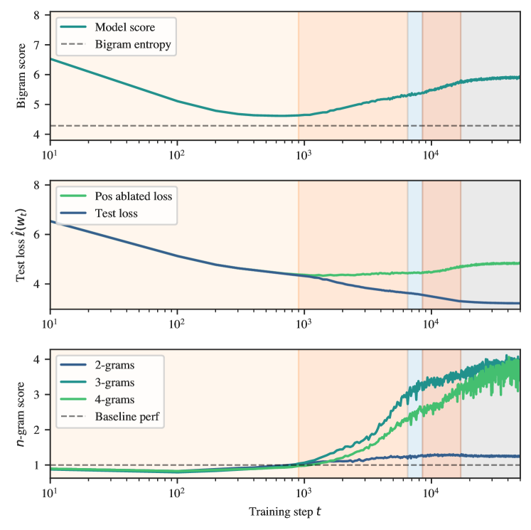
Figure 3: The language transformer learns bigram statistics in LM1 (top). At the start of LM2, the positional embedding suddenly becomes useful (middle), enabling behavioral changes such as the learning of common $n$-grams (bottom).

4.2 Stage LM2 (900–6.5k steps)

Behavioral changes.

A natural next step after bigrams are $n$-grams, token sequences of length $n$. We define an $n$-gram score as the ratio of final-position token loss on (1) a baseline set of samples from a validation set truncated to $n$ tokens and (2) a fixed set of common $n$-grams (see Section C.2.2). We see a large improvement in $n$-gram score for $n=3,4$ in Figure 3 (bottom), rising to several times the baseline ratio ($1.0$). Although this is one natural next step for the learning process, we do not rule out other possible developmental changes for this stage, such as skip-trigrams.

Structural changes.

The positional embedding is necessary for learning $n$-grams, and, as expected, the model becomes dependent on the positional embedding during LM2. This is apparent in comparing the test loss with and without the positional embedding zero-ablated in Figure 3 (middle) — the curves are indistinguishable at first but diverge at the LM1–LM2 boundary (see Section C.3.1). We also see a rise in previous-token attention among second layer attention heads in the background of Figure 4 (top), which we also suspect plays a role with $n$-grams.

Interestingly, even before the heads that eventually become induction heads develop their characteristic attention patterns in stages LM3 and LM4, they begin to compose (that is, read and write from the same residual stream subspace) near the start of stage LM2 (see Figures 20 and C.3.2). This suggests that the foundations of the induction circuit model are laid well in advance of any measurable change in model outputs or attention activations.

4.3 Stage LM3 (6.5k–8.5k steps)

Structural changes.

First-layer previous-token heads, the first half of induction circuits, begin to form Elhage et al. (2021). Figure 4 (top) shows that the fraction these heads (highlighted in blue) attend to the immediately preceding token begins to increase during this stage (see Section C.3.3).

During this stage the LLC decreases, suggesting an increase in degeneracy and decrease in model complexity, perhaps related to the interaction between heads. It would be interesting to study this further via mechanistic interpretability.

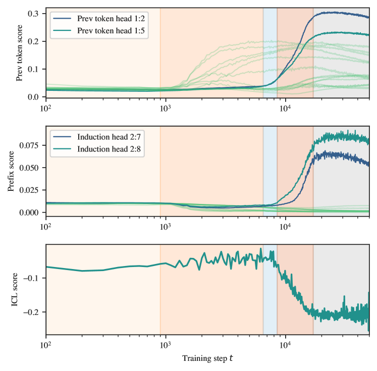
Figure 4: Induction circuit formation begins with previous-token heads (LM3, top), followed by induction heads (LM4, middle), which leads to a drop in ICL score (LM4, bottom). The $h$th attention head in layer $l$ is indexed as $l:h$.

4.4 Stage LM4 (8.5k–17k steps)

Behavioral changes.

The model learns to perform ICL as studied by Olsson et al. (2022) (Figure 4 bottom).

Structural changes.

The second half of the induction circuits, second-layer induction heads, begin to develop. Given a sequence $[A][B]\ldots[A]$, the prefix-matching score of Olsson et al. (2022) measures attention to $[B]$ from the latter $[A]$ (see Section C.3.4). Figure 4 (middle) shows that the prefix-matching score begins to increase for the two heads that become induction heads (highlighted in blue).

5 Results for Linear Regression

In the linear regression setting, plateaus in the LLC estimate (Figures 1(b) and 2) reveal five developmental stages, corresponding to learning the task prior (LR1), acquiring in-context learning (LR2), and “over-fitting” to the input distribution (LR3/LR4). Forms in the ED (Figure 2(b) and Figure 6(b)) corroborate the LR1–LR2, LR2–LR3 and LR3–LR4 boundaries. Near-plateaus in the LLC, an additional form in the ED and other metrics suggest that LR2, LR3, and LR4 can be divided into additional substages (Section D.1.4).

The positions of these milestones vary slightly between runs, but the overall ordering is preserved. In this section, we present results for the regression transformer trained from seed $1$ (“$\lrt{1}$”). For other training runs, see Appendix F.

5.1 Stage LR1 (0–1k steps)

Behavioral changes.

Similar to bigrams in the language model setting, the model learns the optimal context-independent algorithm, which is to predict using the average task $\bar{\task}$, which is zero for our regression setup. Figure 5 shows that the average square prediction for all tokens $\mathbb{E}[\|\hat{y}_{k}\|^{2}]$ approaches zero during LR1, reaching a minimum slightly after the end of LR1of $0.1$ (which is smaller than the target noise $\sigma^{2}=0.125$).

5.2 Stage LR2 (1k–40k steps)

Behavioral changes.

The model acquires in-context learning during this stage (Figure 5 bottom, with $g=1$). This parallels stage LM4 in the the language model setting.

Structural changes.

The token and positional embedding begin to “collapse” towards the end of this stage, effectively losing singular values and aligning with the same activation subspace (Section D.3.1). At the same time, several attention heads form distinct and consistent patterns (Section D.3.5).

5.3 Stages LR3 & LR4 (40k–126k & 126k–320k steps)

Behavioral changes.

The model begins to “overfit” to the input distribution. Performance continues to improve on typical samples, but deteriorates on extreme samples for which the norm of the inputs $x_{k}$ is larger than encountered in during training.

Structural changes.

During these stages, the layer norm weights undergo a phenomenon we term layer norm collapse, in which a large fraction of the layer norm weights rapidly go to zero (Section D.3.4). This phenomenon is most pronounced in the unembedding layer norm, where it occurs in tandem with a similar collapse in the weights of the unembedding matrix (Section D.3.3). This results in the model learning to read its final prediction from a handful of privileged dimensions of the residual stream. These observations, which point to concrete examples of degeneracy in the network parameter, may explain part of the observed LLC decrease over these stages.

Stage LR4 differs from LR3 in the layer norm collapse expanding from the unembedding to earlier layer norms, particularly the layer norm before the first attention block. This affects a smaller fraction of weights than the unembedding collapse.

Figure 5: Top: During LR1, the model learns to predict with the task prior, $x_{k}\mapsto\hat{y}_{k}=0$. Bottom: ICL emerges during LR2. In LR3, the model becomes worse at ICL on out-of-distribution inputs $x_{k}\sim\mathcal{N}(0,gI_{D})$.

6 Discussion and Related Work

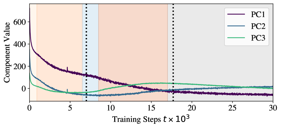
(a) Two-Layer Attention-only Language Transformer.

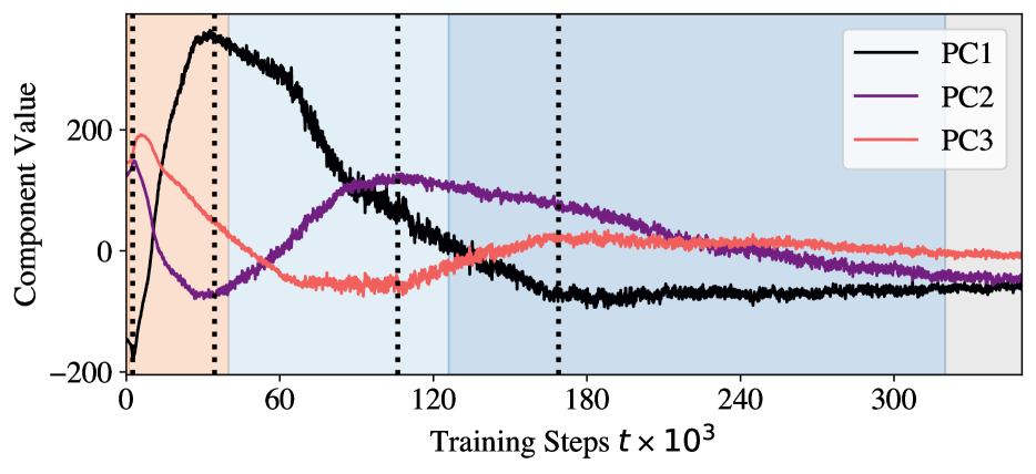
(b) Linear Regression Transformer.

Figure 6: The PC scores over time from ED for each setting, with forms marked by dashed lines at the timesteps given in Table 1, Table 2. This shows the alignment between stage boundaries set by LLC and the forms of the developmental trajectory (and suggests a possible substage in LR4, see Section D.1.4). Note that local extrema of the PC scores occur near the timesteps associated with forms, see Section B.6.

Stage-wise development.

The study of stage-wise development in artificial neural networks spans several decades (Raijmakers et al., 1996). It has long been known that in simple (linear) neural networks, these stages can be linked to “modes” of the data distribution, meaning eigenvectors of covariance matrices (Baldi & Hornik, 1989; Rogers & McClelland, 2004; Saxe et al., 2019). In our experiments some of the early stages, such as learning bigrams (LM1), can be understood as learning modes in this sense. With the observation of emergent phenomena in neural network training (Wei et al., 2022; Olsson et al., 2022; McGrath et al., 2022) these ideas have attracted renewed attention.

Developmental biology and bifurcations.

We have emphasized changes in geometry over a stage whereas in developmental biology the focus, in the mathematical framework of bifurcation theory, is more on the singular geometry at milestones (Rand et al., 2021; MacArthur, 2022; Sáez et al., 2022). The relationship between these two points of view is beyond the scope of this paper. For more on the relation between the points of view of Waddington and Thom, see (Franceschelli, 2010).

Loss landscape geometry.

Many authors have used one or two-dimensional slices of the loss landscape to visualize its geometry (Erhan et al., 2010; Goodfellow et al., 2014; Lipton, 2016; Li et al., 2018; Notsawo et al., 2023). These approaches are limited by the fact that a random slice is with high probability a quadratic form associated to nonzero eigenvalues of the Hessian and is thus biased against important geometric features, such as degeneracy. The LLC and ED are able to probe such degenerate geometry in a quantitative way.

Trajectory PCA.

The use of trajectory PCA to study structural development in transformers was initiated by Olsson et al. (2022), who were the first to observe the vertex in $\gamma_{1,2}$ which we show is part of the first form in the language modeling setting (due to their using a small number of checkpoints, what we observe to be a vertex appears as a sharp point there). This feature was observed in transformers ranging in scale up to 13B parameters, suggesting the ED method can be scaled substantially.

Progress measures.

Barak et al. (2022) show in a special setting that there are progress measures for neural network learning that reflect hidden continuous progress invisible to loss and error metrics, and which may precede phase transitions. The structural and behavioral indicators used here resemble the progress measures investigated by Nanda et al. (2023) in the context of reverse-engineering transformers trained on modular arithmetic. The LLC and ED differ in not requiring prior knowledge of what is changing during a stage. As we’ve demonstrated, the developmental and mechanistic approaches are complementary.

Algorithmic compression.

It is natural to interpret a stage in which the LLC decreases as a simplification or compression of an existing algorithm. Our observation of Type B stages is consistent with the literature on grokking (Nanda et al., 2023). In the linear regression setting the collapse of layer norm (Section D.3.4), embedding (Section D.3.1), and attention patterns (Section D.3.5) seem to be involved, but at present the evidence for this is not conclusive.

Universality.

Olah et al. (2020) hypothesize that similar internal structures may form across a wide range of different neural network architectures, training runs, and datasets. Examples of such preserved structures include Gabor filters, induction heads, and “backup heads” (Olah et al., 2020; McGrath et al., 2023; Wang et al., 2022). In our linear regression setting, we observe a stronger form of universality, in which the order of developmental stages appears to be preserved. The abstract structure which jointly organizes the macroscopic similarities between these processes is what we refer to as the developmental landscape, following Waddington (1957). Though we do not expect all aspects of development to be universal, we conjecture that the developmental trajectory will remain macroscopically simple even for much larger models.

7 Conclusion

Transformers undergo stage-wise development.

We identified five developmental stages in the setting of transformers trained on natural language modeling and five in synthetic linear regression tasks. These stages are distinguished by the local learning coefficient, geometric features of the developmental trajectory in essential dynamics, and a range of other data- and model-specific metrics.

Stages are detected by the LLC and ED, which are scalable data- and model-agnostic developmental indicators.

Many stages are not visible in the loss. While a stage may be easily isolated once you know the right data-specific metric (e.g. the cross entropy with bigram frequencies for LM1) these post-hoc metrics depend on knowing that the stage exists and some of its content. In contrast, the LLC and ED can be used to discover developmental stages.

Future work: developmental interpretability.

Studying neural network development helps to interpret the structure of the final trained network, since we can observe the context in which that structure emerges. We expect that LLC and ED, applied over the course of training in the manner pioneered in this paper, will aid in discovering and interpreting structure in other neural networks.

Appendix

• Appendix A reviews SGLD-based LLC estimation Lau et al. (2023). It provides some simple toy examples contrasting the learning coefficient and Hessian-based measures and ends with a discussion on using LLC estimation to detect developmental milestones.

• Appendix B covers the theoretical foundations of essential dynamics. It discusses vertices and forms, provides a toy example of what they mean, and covers their relation to PCA, ending with a discussion on common pitfalls of PCA.

• Appendix C and Appendix D examine the developmental stages of language and linear regression in more detail and explain the various indicators we use to track geometric, behavioral, and structural development.

• Appendix E covers experimental details, such as model architecture, training procedure, and hyperparameters for LLC estimation and ED. We end this section with a worked through treatment of the calibrations involved in applying LLC estimation to regression transformers as a reference (Section E.3).

• Appendix F contains a link to additional figures and the codebase used to run the experiments in this paper.

Appendix A LLC

A.1 Examples of the LLC

Given a model $p$, truth $q$ and a point $w^{*}\in W\subseteq\mathbb{R}^{d}$ in parameter space, the LLC quantifies the degree to which $w$ can be varied near $w^{*}$ in such a way that the model $p(x|w)$ stays close to $p(x|w^{*})$, relative to the truth (Watanabe, 2009, §7.1). It can also be interpreted as a measure of model complexity, given its role in the asymptotic expansion of the local free energy (Watanabe, 2009).

The notion has some similarity to an effective parameter count. If the population log likelihood $L$ looks like a quadratic form near $w^{*}$ then $\lambda(w^{*})=\tfrac{d}{2}$ is half the number of parameters, which we can think of as $d$ contributions of $\tfrac{1}{2}$ from every independent quadratic direction. If there are only $d-1$ independent quadratic directions, and one coordinate $w_{i}$ such that small variations in $w_{i}$ near $w_{i}^{*}$ do not change the model relative to the truth (it is “unused”) then $\lambda(w^{*})=\tfrac{d-1}{2}$. However, while every unused coordinate reduces the LLC by $\tfrac{1}{2}$, changing a coordinate from quadratic $w_{i}^{2}$ to quartic $w_{i}^{4}$ (increasing its degeneracy while still “using” it) reduces the contribution to the LLC from $\tfrac{1}{2}$ to $\tfrac{1}{4}$.

As a source of intuition, we provide several examples of exact local learning coefficients for toy loss functions:

• $L(w_{1},w_{2},w_{3})=aw_{1}^{2}+bw_{2}^{2}+cw_{3}^{2}$ with $a,b,c>0$. This function is nondegenerate, and $\lambda(0,0,0)=\tfrac{1}{2}+\tfrac{1}{2}+\tfrac{1}{2}=\tfrac{3}{2}$. This is independent of $a,b,c$. That is, the LLC $\lambda$ does not measure curvature. For this reason, it is better to avoid an intuition that centers on “basin broadness” since this tends to suggest that lowering $a,b,c$ should affect the LLC.

• $L(w_{1},w_{2},w_{3})=w_{1}^{2}+w_{2}^{2}+0$ in $\mathbb{R}^{3}$ is degenerate, but its level sets are still submanifolds and $\lambda(0,0,0)=\tfrac{1}{2}+\tfrac{1}{2}$. In this case the variable $z$ is unused, and so does not contribute to the LLC.

• $L(w_{1},w_{2},w_{3})=w_{1}^{2}+w_{2}^{4}+w_{3}^{4}$ is degenerate and its level sets are, for our purposes, not submanifolds. The singular function germ $(L,\mathbf{0})$ is an object of algebraic geometry, and the appropriate mathematical object is not a manifold or a variety but a scheme. The quartic terms contribute $\tfrac{1}{4}$ to the LLC, so that $\lambda(0,0,0)=\tfrac{1}{2}+\tfrac{1}{4}+\tfrac{1}{4}=1$. The higher the power of a variable, the greater the degeneracy and the lower the LLC.

For additional examples (still far from exhaustive), see Figure 7. While nondegenerate functions can be locally written as quadratic forms by the Morse Lemma (and are thus qualitatively similar to the approximation obtained from their Hessians), there is no simple equivalent for degenerate functions, such as the population log likelihood of singular models (or population losses of neural networks). We refer the reader to Watanabe (2009) and Lau et al. (2023) for more discussion.

Figure 7: Toy two-dimensional loss landscapes show that the lower the LLC, the more the local geometry deviates from quadratic. Left: A quadratic potential $L_{1}(w_{1},w_{2})=w_{1}^{2}+w_{2}^{2}$, for which the LLC is maximal in two dimensions, $\lambda_{1}(0,0)=d/2=1$. Middle-left: A quartic potential $L_{2}(w_{1},w_{2})=w_{1}^{4}+w_{2}^{4}$, for which the LLC is $\lambda_{2}(0,0)=1/2$. Middle-right: An even simpler potential $L_{3}(w_{1},w_{2})=w_{1}^{2}w_{2}^{4}$, for which $\lambda_{3}(0,0)=1/4$. Hessian-derived metrics cannot distinguish between this geometry and the preceding quartic geometry. Right: A qualitatively distinct potential $L_{4}(w_{1},w_{2})=(w_{1}-1)^{2}(w_{1}^{2}+w_{2}^{2})^{4}$ from Lau et al. (2023) with the same LLC at the origin, $\lambda_{4}(0,0)=1/4$.

A.2 Phase Transitions and Developmental Stages

Singular learning theory offers some theoretical context for the phenomena we observe in our experiments. The free energy formula (Watanabe, 2009) says, in the local setting (Chen et al., 2023), that for a region $W_{\alpha}$ of parameter space dominated by a local minima $w_{\alpha}^{*}$ of the log likelihood $L$, the free energy has an asymptotic expansion in the number of samples $n$

$$F_{n}(W_{\alpha})\approx nL_{n}(w_{\alpha}^{*})+\lambda(w_{\alpha}^{*})\log n+c_{\alpha}$$ (8)

where $c_{\alpha}$ consists of terms of constant order or lower (for simplicity we ignore $\log\log n$ terms). On general principles, we expect the Bayesian posterior to shift from region $W_{\alpha}$ to region $W_{\beta}$ as $n$ increases, when:

• $w_{\beta}^{*}$ has lower loss, but higher complexity than $w_{\alpha}^{*}$. That is, $L(w_{\beta}^{*})<L(w_{\alpha}^{*})$ and $\lambda(w_{\beta}^{*})>\lambda(w_{\alpha}^{*})$. Note that for small $n$, the loss is large and the LLC is small.

• $w_{\beta}^{*}$ has similar loss, but lower complexity than $w_{\alpha}^{*}$. That is, $L(w_{\beta}^{*})\approx L(w_{\alpha}^{*})$ and $\lambda(w_{\beta}^{*})<\lambda(w_{\alpha}^{*})$.

The connection between the Bayesian learning process (the shift of the Bayesian posterior as $n$ increases) and the learning process of SGD remains unclear, although in some cases they are known to be related (Chen et al., 2023). Nonetheless, it is notable that stages LR1, LR2, and LR5 in the linear regression setting and stages LM1, LM2, LM4, and LM5 in the language modeling setting are of Type A, while stages LR3, LR4, and LM3 are of Type B.

While phase transitions are sometimes characterized as “sudden,” from a mathematical point of view (Chen et al., 2023; Gilmore, 1981) the important characteristic of a phase transition is that the configuration of a system (or a distribution over such configurations) shifts rapidly from a neighborhood of one critical point of a relevant potential (e.g. a free energy) to another critical point, as a function of some control variable $c$ near some critical value $c\approx c_{0}$. To take one example: in developmental biology there are carefully modeled phase transitions which take place over days in real time. The relevant control variable in these cases is an inferred developmental time $\tau=\tau(t)$ Freedman et al. (2023). Because “phase transition” retains the false connotation of being sudden in time, we borrow from biology in referring to “developmental stages.”

A.3 Log Likelihood-Based Loss

In the main body, we apply the LLC to loss functions that do not arise as the log likelihood of independent random variables, due to the repeated use of dependent subsequences. Here we show how it is in fact possible to define a proper negative log likelihood over independent observations for our two motivating problems. Let’s see how this plays out specifically for the linear regression setting. Let $\Pi(k)$ be a probability distribution over the context length $k$. Ideally, the transformer would be trained to make predictions $y_{k}$ given a context of length $k$ where $k$ is sampled from $\Pi$. By ideal, we simply mean that training on sequences of varying length $k$ will allow the transformer to handle prompts of different lengths at inference time. This would lead to the population loss

$$\ell(w)=\sum_{k}p_{k}\ell_{k}(w)$$ (9)

where $p_{k}$ is the probability of sampling $k$ from $\Pi$ and

$$\ell_{k}(w)=\int q(S_{k},y_{k}|\task,k)q(\task)\Big{[}f_{w}(S_{k})-y_{k}\Big{]}^{2}\,dS_{k}\,dy_{k}\,d\task.$$ (10)

Figure 8 depicts LLC traces (Section E.3) for a highlighted number of checkpoints using either a likelihood-based estimate (with variable sequence length) or loss-based estimate (with fixed sequence length). The relative orderings of complexities does not change, and even the values of the LLC estimates do not make much of a difference, except at the final checkpoint, which has a higher value for the subsequence-based estimate.

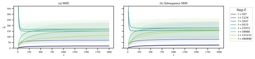
Figure 8: Loss-based (left) and likelihood-based (right) LLC estimation yield identically ordered LLC estimates. With the exception of final checkpoint’s LLC estimate (which is larger for the loss-based estimate), the values are close to identical. These plots display LLC traces, which show the LLC estimate as a function of SGLD steps. This is a useful tool for calibrating LLC estimation (Section E.3).

A.4 Estimating LLCs with SGLD

We follow Lau et al. (2023) in using SGLD to estimate the expectation value of the loss/negative log likelihood in the expression for the local learning coefficient. For a given choice of weights $w^{*}$ we sample $C$ independent chains, indexed by $c$ with $T_{\mathrm{SGLD}}$ steps per chain. For each chain, we draw a set of weights $\{w^{(c)}_{\tau}\}_{\tau=1}^{T_{\mathrm{SGLD}}}$. From these samples, we estimate the expectation of an observable $\mathcal{O}$ by

$$\mathbb{E}^{\beta}_{w|w^{*},\gamma}[\mathcal{O}(w)]\approx\frac{1}{CT_{\mathrm{SGLD}}}\sum_{c=1}^{C}\sum_{\tau=1}^{T_{\mathrm{SGLD}}}\mathcal{O}(w_{\tau,\beta,\gamma}^{(c)}),$$ (11)

with an optional burn-in period and thinning.

Dropping the chain index $c$ and the explicit dependence on $\beta$ and $\gamma$, each sample is generated according to:

$$w_{\tau+1} =w_{\tau}+\Delta w_{\tau},$$ (12)

$$w_{1} =w^{*},$$ (13)

where the step $\Delta w_{\tau}$ comes from minibatch-SGLD,

$$\Delta w_{\tau}=\frac{\epsilon}{2}\left(\beta n\nabla\batchloss[(\tau)](w_{\tau})+\gamma\left(w_{\tau}-w^{*}\right)\right)+\mathcal{N}(0,\epsilon),$$ (14)

over minibatch losses $\batchloss[(\tau)]$ for minibatches of size $m$, drawn from the dataset $D_{n}$. Similar to Lau et al. (2023), for reasons of efficiency, we recycle the batch losses for the average rather than computing the full-batch loss for each SGLD draw. That is, we take $\mathcal{O}=L_{m}^{(\tau)}$ rather than $\mathcal{O}=L_{n}$. More detailed results for language and regression are provided in Section C.1 and Section D.1, respectively. Section E.3 provides a walk-through for the LLC calibration process in the regression transformers.

A.5 Automated Stage Discovery

To identify stage boundaries, we look for plateaus in the LLC: checkpoints at which the slope of $\hat{\lambda}(w_{t})$ over $t$ vanishes. To mitigate noise in the LLC estimates, we first fit a Gaussian process with some smoothing to the LLC-over-time curve. Then we numerically calculate the slope of this Gaussian process with respect to $\log t$. The logarithm corrects for the fact that the learning coefficient, like the loss, changes less as training progresses. We identify milestones by looking for checkpoints at which this estimated slope equals zero. The results of this procedure are depicted in Figure 12 for language and Figure 23 for linear regression.

At a boundary between a type-A and type-B transition (Section A.2), identifying a plateau from this estimated slope is straightforward, since the derivative crosses the x-axis. At a boundary between two transitions of the same type, the slope does not exactly reach zero, so we have to specify a “tolerance” for the absolute value of the derivative, below which we treat the boundary as an effective plateau. In this case, we additionally require that the plateau be at a local minimum of the absolute first derivative. Otherwise, we may identify several adjacent points as all constituting a stage boundary.

To summarize, identifying stage boundaries is sensitive to the following choices: the intervals between checkpoints, the amount of smoothing, whether to differentiate with respect to $t$ or $\log t$, and the choice of tolerance. However, once a given choice of these hyperparameters is fixed, stages can be automatically identified, without further human judgment.

In Section D.1.4, we consider what happens upon relaxing the choice of threshold in the linear regression setting. We find this leads to several additional candidate milestones.

A.6 LLC Estimates Away from Local Minima

Our methodology for detecting stages is to apply LLC estimation to compute $\hat{\lambda}(w^{*})$ at neural network parameters $w^{*}=w_{t}$ across training. In the typical case these parameters will not be local minima of the population loss, violating the theoretical conditions under which $\hat{\lambda}$ is a valid estimator of the true local learning coefficient (Lau et al., 2023).

This makes it a priori quite surprising that the SGLD-based estimation procedure works at all, as away from local minima, one might expect the chains to explore directions in which the loss decreases. Beyond that, critical points in the $\hat{\lambda}(w_{t})$ curve do correspond to meaningful changes in the mode of development in our experiments.

This raises an interesting theoretical question: is there a notion of stably evolving equilibrium in the setting of neural network training, echoing some of the ideas of Waddington (1957), such that the LLC estimation procedure is effectively giving us the local learning coefficient of a different potential to the population loss, a potential for which the current parameter actually is at a critical point? We view the discussion in Section B.4 and Section B.5 as providing some evidence for this view. However at the moment we must admit that our methodology goes beyond what is justified by the theoretical foundations.

Appendix B Essential Dynamics

We supplement Section 3.2 with a theoretical development of vertices of developmental trajectories and their relation to progress measures (Barak et al., 2022; Nanda et al., 2023). Relevant background on geometry of curves can be found in Bruce & Giblin (1992). In particular we assume familiarity with the notion of an osculating circle (the best approximating circle to a curve at a point, whose radius is inverse to the curvature at the point).

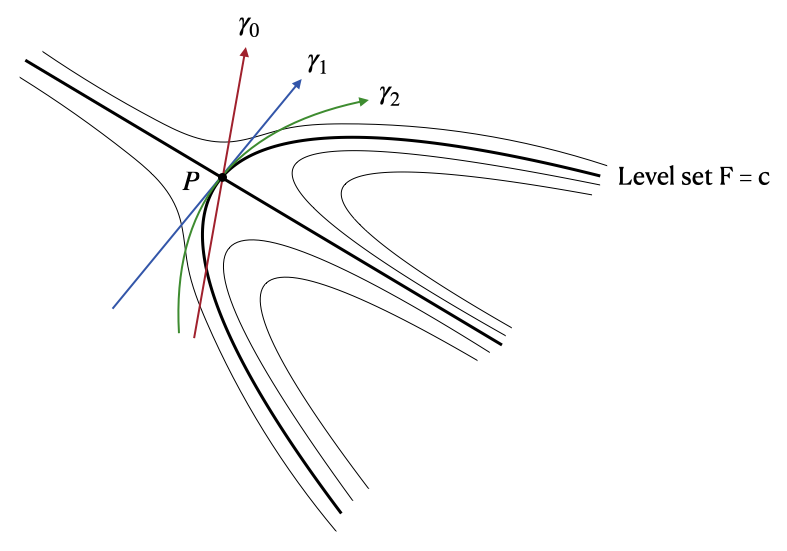
Figure 9: A visualization of the order of contact of three curves $\gamma_{i}$ with the level set $F=c$ of a function $F$ at $P$. This level set (bold) has two irreducible components: a line $L$ and a curve $C$ which meet at $P$. Other nearby level sets are shown as black lines. The curve $\gamma_{0}$ has contact order $1$ (passes through $P$ but is not tangent to the level set at $P$), the curve $\gamma_{1}$ has second order contact (tangent to the curve $C$ at $P$ but disagreeing at second order) while the curve $\gamma_{2}$ has order $\geq 3$. The higher the order of contact with the level set, the more the curve “behaves like” a component.

B.1 Vertices

We refer to (Bruce & Giblin, 1992, Ch. 2) for more background on contact and vertices.

Definition B.1.

Given a smooth function $F:\mathbb{R}^{v}\rightarrow\mathbb{R}$ and smooth curve $\gamma$ in $\mathbb{R}^{v}$ the order of contact of $\gamma$ at $t=t_{0}$ with a level set $F^{-1}(c)$ is defined to be $\geq k$ if

$$\frac{d^{i}}{dt^{i}}(\bar{F}\circ\gamma)\big{|}_{t=t_{0}}=0\quad 0\leq i\leq k-1$$ (15)

where $\bar{F}=F-c$. The order of contact is defined to be equal to $k$ if it is $\geq k$ but not $\geq k+1$.

This quantity is still meaningful when the level set is not a manifold. Order of contact is a formal way of saying that the trajectory $\gamma$ is aligned with the geometry of the level sets of $F$, see Figure 9. For a simple example, consider $\gamma(t)=(t,1-t^{2})$ in $\mathbb{R}^{2}$ and the smooth function $F(x,y)=x^{2}+(y-\tfrac{1}{2})^{2}$. We have

$$F(\gamma(t))=t^{2}+(\tfrac{1}{2}-t^{2})^{2}=\tfrac{1}{4}+t^{4}$$

which satisfies $\frac{d^{i}}{dt^{i}}(\bar{F}\circ\gamma)\big{|}_{t=0}=0$ for $0\leq i\leq 3$ but the fourth derivative is nonzero, where $\bar{F}=F-\tfrac{1}{4}$. So $\gamma$ has contact of order $4$ with the level set $F^{-1}(\tfrac{1}{4})$, that is, with a circle of radius $\tfrac{1}{2}$ centered at $(0,\tfrac{1}{2})$.

We can talk about contact of smooth curves in $\mathbb{R}^{v}$ with level sets of distance functions $\|x-Q\|^{2}$ for points $Q\in\mathbb{R}^{v}$, for any $v$, but in two dimensions such contact is given a special name:

Definition B.2.

A vertex of a plane curve $\gamma$ is a parameter value $t=t_{0}$ such that for some $Q\in\mathbb{R}^{2}$ the curve $\gamma$ has order of contact $\geq 4$ at $t=t_{0}$ with a level set of the function

$$F(x)=\|x-Q\|^{2}\,.$$

We say that $\gamma$ has a vertex at $t_{0}$, or less precisely, at $P=\gamma(t_{0})$. We refer to $Q$ as the center of the osculating circle at $t=t_{0}$. If the contact order is exactly $4$ we call this an ordinary vertex. The notion of contact is intrinsic to the plane curve and does not depend on the parametrization.

So the smooth curve $\gamma(t)=(t,1-t^{2})$ has an ordinary vertex at $t=0$ with osculating circle centered on $(0,1)$.

In the definition we implicitly assume that $Q$ is not equal to $\gamma(t_{0})$, that is, that the relevant level set of $F$ is not the zero level set. However this is an interesting limiting case that we actually encounter in the main text, so it needs examination. The next lemma says that certain kinds of degenerate singularities are limiting cases of vertices.

Lemma B.3.

A plane curve $\gamma$ has contact of order $4$ with the function $F(x)=\|x-\gamma(t_{0})\|^{2}$ at $t=t_{0}$ if and only if

$$\gamma^{\prime}(t_{0})=\gamma^{\prime\prime}(t_{0})=0\,.$$

That is, $\gamma$ has a cusp singularity at $t=t_{0}$.

Proof.

Set $Q=\gamma(t_{0})$. The condition for contact of order $\geq k$ says

$$\frac{d^{i}}{dt^{i}}\|\gamma(t)-Q\|^{2}\big{|}_{t=t_{0}}=0\,,\qquad 0\leq i\leq k-1$$ (16)

which is equivalent to

$$\frac{d^{i}}{dt^{i}}\langle\gamma-Q,\gamma^{\prime}\rangle\big{|}_{t=t_{0}}=0\,,\qquad 0\leq i\leq k-2\,.$$ (17)

Distributing the derivatives inside the pairing gives

$$\sum_{a+b=i}\binom{i}{a}\Big{\langle}\frac{d^{a}}{dt^{a}}(\gamma-Q),\frac{d^{b+1}}{dt^{b+1}}\gamma\Big{\rangle}\Big{|}_{t=t_{0}}=0\,,\qquad 0\leq i\leq k-2\,.$$ (18)

Noting that $(\gamma-Q)\big{|}_{t=t_{0}}=0$, summands with $a=0$ vanish and so

$$\sum_{a+b=i,a\geq 1}\binom{i}{a}\Big{\langle}\frac{d^{a}}{dt^{a}}\gamma,\frac{d^{b+1}}{dt^{b+1}}\gamma\Big{\rangle}\Big{|}_{t=t_{0}}=0\,,\qquad 0\leq i\leq k-2\,.$$

When $k=4$ we have the following equations for $i=1,2,3$, where all functions are evaluated at $t=t_{0}$

$$\|\gamma^{\prime}\|^{2}=0\,,$$

$$2\langle\gamma^{\prime},\gamma^{\prime\prime}\rangle+\langle\gamma^{\prime\prime},\gamma^{\prime}\rangle=0\,,$$

$$3\langle\gamma^{\prime},\gamma^{\prime\prime\prime}\rangle+3\langle\gamma^{\prime\prime},\gamma^{\prime\prime}\rangle+\langle\gamma^{\prime\prime\prime},\gamma^{\prime}\rangle=0\,.$$

It is easy to see that these hold if and only if the conditions stated in the lemma hold. ∎

B.2 Two Kinds of Geometry

We now specialize to the situation described in Section 3.2.1 and sketch the connection between the two kinds of geometry considered in this paper: geometry in parameter space and geometry in function space. We assume a neural network $f_{w}$ is given with outputs in $\mathbb{R}^{m}$ and that $I=\{x_{i}\}_{i=1}^{n}$ is a finite set of inputs. We consider the function space $\mathcal{F}=(\mathbb{R}^{m})^{I}$ with its usual Hilbert space structure $\langle f,g\rangle=\sum_{i=1}^{n}f(i)g(i)$. We consider distance-squared functions of the form

$$F(f,f^{*})=\|f-f^{*}\|^{2}\,,$$

where $f,f^{*}\in\mathcal{F}$. By definition of the norm

$$F(f_{w},f^{*})=\sum_{i=1}^{n}(f_{w}(x_{i})-f^{*}(x_{i}))^{2}\,,\qquad w\in W\,.$$ (19)

Suppose that $f^{*}$ is the true function, so that $\ell_{n}(w)=F(f_{w},f^{*})$ is the MSE for $D_{n}=I$. If $w=w(t)$ is a smooth path in the parameter space $W$ and $\gamma(t)=f_{w(t)}$ then $F(\gamma(t))=\ell_{n}(w(t))$ so that $\gamma$ has contact of order $\geq k$ with a level set of $F$ if and only if $w$ has contact of order $\geq k$ with a level set of $\ell_{n}$. This sets up a simple connection between geometry of the developmental trajectory in function space and how the geometry of the loss landscape interacts with the trajectory in the space of weights. As we take $n\rightarrow\infty$ we see a connection between the geometry of the population loss function $\ell$ and the geometry of the developmental trajectory in $L^{2}(X,q(x))$ where $X$ is the sample space and $q(x)$ the input distribution.

B.3 Inferring Forms from Vertices

In the setting of Section B.2 let $u_{1},\ldots,u_{v}$ be an orthonormal basis for a subspace $V$ of the function space $\mathcal{F}$ and write

$$\gamma(t)=\sum_{a=1}^{v}\gamma_{a}(t)u_{a}$$

for a smooth curve in $V$. With $\pi_{i,j}$ denoting the projection to $\mathbb{R}^{2}$ using the pair $u_{i},u_{j}$ for $i<j$, let $\gamma_{i,j}(t)=\pi_{i,j}(\gamma(t))$.

Lemma B.4.

If at $t=t_{0}$ each of the plane curves $\gamma_{i,j}(t)$ for $i<j$ has a vertex, and moreover these vertices can be lifted by which we mean that there exists $Q=\sum_{a}q_{a}u_{a}$ such that $Q_{i,j}=(q_{i},q_{j})$ is the center of the osculating circle to $\gamma_{i,j}$ at $t=t_{0}$, then $\gamma$ has order of contact $4$ in $V$ with the squared distance function

$$F(f)=\|f-Q\|^{2}\,.$$

Proof.

We actually prove that if each of the $\gamma_{i,j}$ has order of contact $\geq k$ then so does the curve in $V$. If this hypothesis holds, then for some constants $Z_{i,j}$

$$\frac{d^{a}}{dt^{a}}\Big{[}\big{(}\gamma_{i}(t)-q_{i}\big{)}^{2}+\big{(}\gamma_{j}(t)-q_{j}\big{)}^{2}-Z_{i,j}\Big{]}\Big{|}_{t=t_{0}}=0\,,\qquad i<j\,\quad 0\leq a\leq k-1\,.$$ (20)

For $a=0$ this just gives the definition $Z_{i,j}:=(\gamma_{i}(t_{0})-q_{i})^{2}+(\gamma_{j}(t_{0})-q_{j})^{2}$, and for $1\leq a\leq k-1$ it can be rewritten as

$$\frac{d^{a}}{dt^{a}}\big{\langle}\pi_{i,j}(\gamma-Q),\pi_{i,j}\gamma^{\prime}\big{\rangle}\Big{|}_{t=t_{0}} =0\quad 0\leq a\leq k-2\,.$$

This is equivalent to

$$\sum_{b+c=a}\binom{a}{b}\Big{\langle}\pi_{i,j}\Big{(}\frac{d^{b}}{dt^{b}}(\gamma-Q)\Big{)},\pi_{i,j}\Big{(}\frac{d^{c}}{dt^{c}}(\gamma^{\prime})\Big{)}\Big{\rangle}\Big{|}_{t=t_{0}}=0\,,\qquad i<j\,\quad 0\leq a\leq k-2$$ (21)

Note that given vectors $A,B\in\mathbb{R}^{v}$ we have $\sum_{i<j}\langle\pi_{i,j}A,\pi_{i,j}B\rangle=(v-1)\langle A,B\rangle$. Hence summing 21 over $i<j$ gives

$$\sum_{b+c=a}\binom{a}{b}\Big{\langle}\frac{d^{b}}{dt^{b}}(\gamma-Q),\frac{d^{c}}{dt^{c}}(\gamma^{\prime})\Big{\rangle}\Big{|}_{t=t_{0}}=0\,,\qquad 0\leq a\leq k-2$$ (22)

which is equivalent to

$$\frac{d^{a}}{dt^{a}}\big{\langle}\gamma-Q,\gamma^{\prime}\big{\rangle}\Big{|}_{t=t_{0}}=0\quad 0\leq a\leq k-2$$ (23)

or what is the same, $\gamma$ has order of contact $\geq k$ with a level set of the squared-distance function $\|f-Q\|^{2}$ in $V$. ∎

We can now define a form and relate it to the informal definition given in Section 3.2.1. We now adopt the setting there, so $\gamma$ is the developmental trajectory in a subspace $V$ of the function space $\mathcal{F}$.

Definition B.5.

A form of the developmental trajectory is a pair $(t_{0},f^{*}_{\alpha})$ where $f^{*}_{\alpha}\in V$ such that the developmental trajectory $\gamma$ in $V$ has contact of order $4$ with a level set of the squared-distance function

$$E_{\alpha}(f)=\|f-f^{*}_{\alpha}\|^{2}$$

at $t=t_{0}$. We refer to $E_{\alpha}$ as the form potential.

Forms are geometric objects in function space: the corresponding geometry in parameter space is the geometry of the form potential, which is “part” of the geometry of the population loss; see Section B.4.

Let us now relate this to the operational definition in the main text. In the main text $v=3$. Let $t=t_{0}$, as in Section 3.2.1, be a timestep at which we observe for all pairs $i<j$ of principal components either a cusp singularity or a vertex in the projected plane curve $\gamma_{i,j}$ at $t=t_{0}$. By a cusp singularity we mean that both the first and second derivatives of $\gamma_{i,j}$ vanish; in practice we look for sharp points where the tangent changes discontinuously. We moreover assume that the centers of the osculating circles to the vertices (which in the case of singularities we take to mean the singular point itself) can be lifted in the sense that there is a single triple $Q=(q_{1},q_{2},q_{3})$ which projects to all these points.

Since such singularities are degenerate cases of vertices (Lemma B.3), Lemma B.4 then applies to show that $\gamma$ has contact of order $4$ with the squared-distance function $\|f-Q\|^{2}$. That is, the point $f^{*}_{\alpha}=Q$ is a form.

B.4 A Toy Model of a Form

Figure 10: The training trajectory can, for some time, prioritise learning about a heuristic $f^{*}_{\alpha}$ in function space.

We describe a simple situation in which a form of the developmental trajectory in the sense of Section 3.2.1 can arise. Informally we suppose that there is a subset of inputs $J\subseteq I$ for which there is a heuristic, which we define loosely to be a solution which is not optimal, but which is accessible in the sense that is easy to change the network parameter in its direction. Our notation is that for a parameter $w\in W$ the neural network function is $f_{w}$, and we let $f^{*}$ denote the target function for the optimization process. We denote by $I$ the finite set of input samples used to construct the developmental trajectory as in Section 3.2, and $\mathbb{R}^{m}$ the space of outputs. Throughout we use $f_{w}$ to denote also the restriction of the neural network to $I$ and subsets of $I$. As in Section B.2 we let $\ell_{n}$ denote the MSE on the dataset $I$.

For a subset $J\subseteq I$ we denote by $\langle-,-\rangle_{J}$ the pairing in the usual Hilbert space structure on $(\mathbb{R}^{m})^{J}$, that is,

$$\big{\langle}f,g\big{\rangle}_{J}=\sum_{x\in J}\big{\langle}f(x),g(x)\big{\rangle}_{\mathbb{R}^{m}}\,.$$

Formally, a heuristic for a subset $J\subseteq I$ is a function $f^{*}_{\alpha}:J\rightarrow\mathbb{R}^{m}$ such that

$$\big{|}\big{\langle}f^{*}_{\alpha}-f_{w},\nabla_{w}f_{w}\big{\rangle}_{J}\big{|}\gg\big{|}\big{\langle}f^{*}-f_{\alpha}^{*},\nabla_{w}f_{w}\big{\rangle}_{J}\big{|}\,.$$ (24)

This is meant to capture a situation like the one in Figure 10 where the directions in which $f_{w}$ can be changed quickly are more aligned with learning $f^{*}_{\alpha}$ than the parts of $f^{*}$ different to $f^{*}_{\alpha}$ (on the inputs $J$). With this hypothesis the gradient of $\ell_{n}$ may be expressed as (where $J^{c}=I\setminus J$)

$$\nabla_{w}\ell_{n}(w) =\nabla_{w}F(f_{w},f^{*})=2\big{\langle}f_{w}-f^{*},\nabla_{w}f_{w}\big{\rangle}$$

$$=2\big{\langle}f_{w}-f^{*},\nabla_{w}f_{w}\big{\rangle}_{J}+2\big{\langle}f_{w}-f^{*},\nabla_{w}f_{w}\big{\rangle}_{J^{c}}$$

$$=2\big{\langle}f_{w}-f^{*}_{\alpha},\nabla_{w}f_{w}\big{\rangle}_{J}+2\big{\langle}f^{*}_{\alpha}-f^{*},\nabla_{w}f_{w}\big{\rangle}_{J}+2\big{\langle}f_{w}-f^{*},\nabla_{w}f_{w}\big{\rangle}_{J^{c}}$$

$$=\nabla_{w}\big{[}E_{\alpha}(w)+S_{\alpha}(w)\big{]}+R_{1}(w)\,.$$

where $\|-\|_{J}$ denotes the norm in $(\mathbb{R}^{m})^{J}$ and

$$E_{\alpha}(w) =\|f_{w}-f_{\alpha}^{*}\|^{2}_{J}$$

$$S_{\alpha}(w) =\|f_{w}-f^{*}\|^{2}_{J^{c}}$$

$$R_{1}(w) =2\big{\langle}f^{*}_{\alpha}-f^{*},\nabla_{w}f_{w}\big{\rangle}_{J}\,.$$

By hypothesis 24, $R_{1}(w)$ is much smaller than the first term, and so

$$\nabla_{w}\ell_{n}(w)\approx\nabla_{w}\big{[}E_{\alpha}(w)+S_{\alpha}(w)\big{]}\,.$$

This divides the gradient into a part from $S_{\alpha}$ which is about learning the true function $f^{*}$ on inputs not in $J$, and a part from $E_{\alpha}$ which is about learning the heuristic on inputs in $J$. We now make an additional assumption, that this divides the learning process into a fast mode which is about learning the heuristic (that is, minimising $E_{\alpha}$) and a slow mode which is about learning everything else (minimising $S_{\alpha}$).

More precisely, we consider a smooth training trajectory $w=w(t)$ which is a solution of the gradient flow equation $w^{\prime}(t)=-\nabla_{w}\ell_{n}(w)$ and assume that on the fast timescale the heuristic is “exhausted” by which we mean $E_{\alpha}(t)=E_{\alpha}(w(t))$ reaches a local minimum as $t\rightarrow t_{0}$ at the same time as the function $S_{\alpha}(t)=S_{\alpha}(w(t))$ continues to slowly decrease. The time $t_{0}$ represents the trajectory reaching the osculating circle in Figure 10. To make connection with vertices of the developmental trajectory we need to insist not only that $E_{\alpha}$ reaches a local minimum, but that this minimum is degenerate

$$\frac{d^{i}}{dt^{i}}E_{\alpha}(t)\big{|}_{t=t_{0}}=0\,,\qquad 1\leq i\leq 3\,.$$

That is, the minimum is quartic rather than quadratic. Under this hypothesis the developmental trajectory, projected onto the function space $(\mathbb{R}^{m})^{J}$, has contact of order $\geq 4$ with the squared-distance function from $f_{\alpha}^{*}$, which is the definition of a form (see Section B.3). Note that in this toy model, the training trajectory $w=w(t)$ does not pass near a critical point of $\ell_{n}$ (since $S_{\alpha}(w)$ steadily decreases) nor does $\gamma(t)=f_{w(t)}$ have a critical point.

The observation that the loss could be a sum of terms, each with their own geometry, is consistent with the work of Barak et al. (2022) and Michaud et al. (2024).

B.5 Milestones Without Critical Points

A standard model of stage-wise development in gradient systems associates milestones to critical points of the governing potential, and stages to paths between these critical points (Gilmore, 1981). This model is widely used in developmental biology (see (Freedman et al., 2023) for a recent example) and is familiar in deep learning under the term “saddle-to-saddle dynamics” (Baldi & Hornik, 1989; Amari, 2016; Jacot et al., 2021). This model of critical points and paths between them would motivate a methodology for detecting of milestones based on looking for singularities $\gamma^{\prime}(t_{0})=0$ of the developmental trajectory, which can associated to critical points of the potential.

However, we do not expect this standard model to apply in general to the development of structure in neural networks. In Figure 1 the test loss curve in the language model setting does not pass through clear plateaus, which might be expected if training has passed close to a critical point. Similarly, we do not see singularities in the developmental trajectory, although some projections are singular. We expect that this is typical of larger models. Our hypothesis instead is that forms, in the sense of Section B.3, are the right general notion rather than critical points; they are, in a certain sense, critical points that are “local” with respect to the data distribution.

B.6 Forms and Principal Components

As defined in Section B.4 forms are rigid objects, and this provides some nontrivial checks on the claims to the existence of forms in Section C.1.2 and Section D.1.2. We stick to the case $v=3$. With the notation of Section B.4, suppose that $u_{1},u_{2},u_{3}$ is an orthonormal basis for $V$ and that $Q=\sum_{a}q_{a}u_{a}$ is such that $Q_{i,j}=(q_{i},q_{j})$ is a cusp singularity or vertex for $\gamma_{i,j}$ at $t=t_{0}$ for all $i<j$. Then we have shown $Q$ is a form, or what is the same

$$\frac{d^{a}}{dt^{a}}\Big{[}\sum_{b=1}^{3}\big{(}\gamma_{b}(t)-q_{b}\big{)}^{2}-\big{\|}\gamma(t_{0})-Q\big{\|}^{2}\Big{]}\Big{|}_{t=t_{0}}=0\,,\qquad 0\leq a\leq 3$$ (25)

However, by hypothesis we also have for every pair $i<j$ that a similar equation holds

$$\frac{d^{a}}{dt^{a}}\Big{[}\big{(}\gamma_{i}(t)-q_{i}\big{)}^{2}+\big{(}\gamma_{j}(t)-q_{j}\big{)}^{2}-\big{\|}\gamma_{i,j}(t_{0})-(q_{i},q_{j})\big{\|}^{2}\Big{]}\Big{|}_{t=t_{0}}=0\,,\qquad 0\leq a\leq 3\,.$$ (26)

Subtracting we deduce that for $1\leq k\leq 3$

$$\frac{d^{a}}{dt^{a}}\Big{[}\big{(}\gamma_{k}(t)-q_{k}\big{)}^{2}-\big{(}\gamma_{k}(t_{0})-q_{k}\big{)}^{2}\Big{]}\Big{|}_{t=t_{0}}=0\,,\qquad 0\leq a\leq 3\,.$$ (27)

This implies a series of three equations which have to hold for all $1\leq k\leq 3$

$$(\gamma_{k}(t_{0})-q_{k})\gamma^{\prime}_{k}(t_{0})=0$$ (28)

$$\gamma^{\prime}_{k}(t_{0})^{2}+(\gamma_{k}(t_{0})-q_{k})\gamma^{\prime\prime}_{k}(t_{0})=0\,,$$ (29)

$$2\gamma^{\prime}_{k}(t_{0})\gamma^{\prime\prime}_{k}(t_{0})+\gamma^{\prime}_{k}(t_{0})\gamma^{\prime\prime}_{k}(t_{0})+(\gamma_{k}(t_{0})-q_{k})\gamma^{\prime\prime\prime}_{k}(t_{0})=0$$ (30)

Let us examine the condition 28. Note that $\gamma_{k}(t)$ are the PC scores, over time, which are shown in Figure 6. The first condition above implies that at a timestep $t_{0}$ associated with a form either $\gamma_{k}(t_{0})=q_{k}$ (the coordinate identified for the form) or this time should be a critical point for the PC score. We now check whether these conditions hold in our two experimental settings.

Linear Regression.

The forms occur at $t_{1}=2.5k,t_{2}=34.5k,t_{3}=106.1k,t_{4}=168.9k$. We denote by $Q_{\alpha}$ the coordinates of form $\alpha$, so that $q_{k}$ above becomes $(Q_{\alpha})_{k}$. The relevant comparisons to check 28 are (leaving aside the PC scores with nearby critical points which satisfy $\gamma^{\prime}_{k}(t_{\alpha})=0$):

$$\gamma_{3}(t_{2})=45\quad vs\quad(Q_{2})_{3}=45\,,$$

$$\gamma_{1}(t_{3})=64\quad vs\quad(Q_{3})_{1}=61\,,$$

$$\gamma_{2}(t_{4})=68\quad vs\quad(Q_{4})_{2}=63\,.$$

Note that the four forms tightly constrain the the PC curves, by dictating the location of their critical points and some of their values. In this way the information in the forms largely determines the shape of the overall developmental trajectory in the three-dimensional projection of function space.

Language modeling.

The forms occur at $t_{1}=7k,t_{2}=17.7k$ and the relevant comparisons are

$$\gamma_{1}(t_{1})=109\quad vs\quad(Q_{1})_{1}=99\,,$$

$$\gamma_{1}(t_{2})=-31\quad vs\quad(Q_{2})_{1}=-21\,,$$

$$\gamma_{2}(t_{2})=33\quad vs\quad(Q_{2})_{2}=33\,.$$

B.7 Pitfalls of PCA

The application of PCA methods to trajectories — related to the continuous-time Functional PCA — requires care, as there are many common failure modes where meaning can be inappropriately assigned to spurious features in PCA trajectories (Antognini & Sohl-Dickstein, 2018; Shinn, 2023).

For this discussion we adopt the notation of Section 3.2 where the data matrix is $A\in\mathbb{R}^{s\times T}$ (with $s>T$ in our setting). The principal component scores $y_{k}\in\mathbb{R}^{T}$ for $k=1,\dots,v$ (where $v<\min(s,T)$) comprise the rows of $Y=PA\in\mathbb{R}^{v\times T}$, where $P\in\mathbb{R}^{v\times s}$ is the PCA projection matrix with the rows corresponding to the top $v$ eigenvectors of the covariance $AA^{T}$, ordered by the magnitude of their corresponding eigenvalues $\lambda_{i}\geq 0$ (which, when normalized, give the explained variance of the principal component). We write $y_{k}(t)=y_{k,t}$ for $t=1,\dots,T$ for convenience.

In examining trajectories of PCA scores $y_{k}(t)$, a non-exhaustive list of illusions one must be aware of include:

1. Lissajous curves: As demonstrated in Antognini & Sohl-Dickstein (2018) and Shinn (2023), the principal component scores of many stochastic processes, in particular high-dimensional Brownian motion and the autoregressive Ornstein-Uhlenbeck process (and their discrete counterparts), have the form $y_{k}(t)\propto\sin(\alpha_{k}t)$ for some constant $\alpha_{k}\propto k$. If these scores are sinusoidal, then plotting parametric curves $(y_{j}(t),y_{k}(t))$ in the plane thus gives rise to Lissajous curves as seen in Figure 11 (bottom row).

   In the context of ED for a model’s trajectory $f_{w_{t}}$ over the course of SGD training, which has both stochastic and autoregressive properties, Lissajous curves in PCA scores should therefore be understood as the null hypothesis. The presence of a turning point at some critical time $t_{c}$ thus does not solely provide evidence for an important developmental event at $t_{c}$.

   Conversely, one can be too conservative in the other direction: seeing Lissajous-like shapes does not automatically make such plots meaningless. It may be the case that only certain stages of development exhibit these sinusoidal PCA scores, which visually outweigh other stages on parametric plots and have an out-sized influence on the explained variance. An important check here is to visualize each $y_{k}(t)$ over time $t$ as done in Figure 11, where it is seen that this periodic behavior is only present for some portions of the trajectory in the top principal components.

2. Artifacts of timescale: If there are not enough checkpoint intervals $T$, then there may be many points of interest in a PCA trajectory which vanish with greater resolution. On top of this, the development of interesting structure in statistical models often takes place over a log-time scale, which means that the practitioner often chooses model checkpoints $t_{1},\dots,t_{T}$ that are spaced by non-linear intervals. While this makes sense from a cost standpoint, it can create artificiality in PCA projections, effectively reducing the resolution near critical times and creating illusory sharp points because of a time-interval that is too coarse. For example what appears to be a sharp point in the PCA plots of (Olsson et al., 2022) appears in our setting (with more resolution) to be a vertex (Figure 2(a)).

Figure 11: The first $v=4$ principal component scores $y_{k}(t)$ (denoted PC1, etc.) for (a) language model (behavioral), (b) linear regression (behavioral), (c) linear regression (weights) and (d) Brownian motion ($s=10000$ dimensions, $n=5000$ timesteps). Notice how in the linear regression and language model settings, many of the principal components only resemble the sinusoidal counterparts of Brownian motion for certain stages of development.

B.8 Smoothing

The developmental trajectory $\gamma$ is a (piece-wise) smooth curve approximating the trajectory computed by projecting the samples $A_{t_{1}},\ldots,A_{t_{T}}$ onto the top principal components. The smoothing is done by applying a Gaussian kernel with standard deviation $\sigma$ to each coordinate. This raises the question of whether the vertices and cusp singularities we observe in the two-dimensional PC plots are “real” or whether they are artifacts of the smoothing.

This explains why in this paper we do not assign any particular meaning to geometric features that are present in only one two-dimensional PC plot (this does not mean they are not meaningful, merely that we do not develop a methodology for arguing that they are). We assign meaning only to forms, which require simultaneous geometric structure across all PC plots; this in itself is nontrivial evidence that each individual structure is not a smoothing artifact.

Once we have inferred the existence of a form (which involves the smoothing process for each curve) we can plot the associated form potentials in Figure 14, Figure 24. These curves show squared-distances in function space from a neural network $f_{w_{t}}$ to the form $f^{*}_{\alpha}$ and do not involve smoothing. The fact that we see highly degenerate critical points (flat bottoms) is by definition evidence for a form, independent of inspection of a two-dimensional PC plot. Finally, the existence of forms is highly constrained, and implies a series of nontrivial constraints on the PC scores across time; verifying these conditions is another check that the inferred forms are genuine (Section B.6).

Altogether, this provides strong evidence that all the forms we have identified are not smoothing artifacts.

Appendix C Developmental Analysis of Language Models

In this section, we present further evidence on the geometric (Section C.1), behavioral (Section C.2), and structural (Section C.3) development of the language model over the course of training. In particular, we investigate and interpret the forms of language model, discovered by ED (Section C.1.3). In addition, we present results for a 1-layer attention-only model (Section C.4).

C.1 Geometric Development

C.1.1 LLC

Figure 12 displays the test loss and LLC curves from Figure 1(a) in addition to the weight norm over time and associated slopes. Stage boundaries coincide with where the slope of the local learning coefficient crosses zero, that is, where there is a plateau in the LLC.

Figure 12: A more detailed version of Figure 1(a) for two-layer language models. Top: Loss, LLC, and weight norm, along with an overlaid Gaussian process fit to these curves (red dotted lines). Bottom: Associated slopes, both numerically estimated finite differences (transparent blue) and of the Gaussian process (red dotted lined). Note that stage LM5 may be subdivided into further stages (Section A.5). However, the noise in LLC estimates late in training is high, so we do not draw any conclusions from this.

C.1.2 Essential Dynamics

(a) Two-Layer Attention-only Language Transformer.

(b) Linear Regression Transformer.

Figure 13: Same as Figure 2 but with the forms of Table 3, Table 4 marked. Green crosses represented the inferred principal components of the form and its associated vertex, while blue crosses mark the beginning and end of the range of influence, which coincides with the vertical marked lines in the form potential plots.

Table 3: Forms for Language Transformer.

Form	Vertex	Influence range	Content	PCs
1	7k	6.5k-10k	New Words	$99,-5,14$
2	17.7k	17.5k-25k	Induction Patterns	$-21,33,30$

Following the algorithm sketched in Section 3.2.1 and made more precise in Section B.3 we identify two forms of the developmental trajectory for the language transformer, the details of which are shown in Table 3. The process of locating the evolute cusps and constructing the values in this table are shown in Figure 13. The associated form potentials are shown in Figure 14. We do not analyze the evolute or forms for $LM5$. For the developmental trajectory of Figure 2 we pre-process the datapoints by smoothing with Gaussian kernel (standard deviation ranging from $50$ initially to $160$ at $t=30\mathrm{k}$) and we then compute osculating circles to this smoothed curve.

C.1.3 Forms

By a token-in-context we mean a pair $(S,p)$ consisting of a sequence $S$ of $1024$ tokens and an index $0\leq p<1024$. The token at the index $p$ is usually denoted with an underline $\underline{[A]}$ throughout this section. We refer to the set of all tokens-in-context by $I$ and denote by $\mathcal{F}$ the space of functions from $I$ to the relevant space of logits.

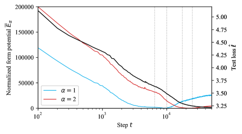
Figure 14: Normalized form potentials $\overline{E}_{\alpha}=E_{\alpha}-\inf_{t}E_{\alpha}(t)$ in the language modeling setting. The flat bottom of the potential, where the trajectory has higher-order contact with a level set of the potential, corresponds to the period where the developmental trajectory moves in a circular orbit in function space around the specified form $f^{*}_{\alpha}$. Note that while the bottom of the curve is a critical point of the potential, the test loss continues to smoothly decrease.

Form 1 ($t=7k$).

To interpret this form we examine extreme logits. That is, we view $f^{*}_{1}$ as a vector of real numbers, compute the mean $\mu$ and standard deviation $\sigma$ and study the extreme entries in the normalized vector $(f^{*}_{1}-\mu)/\sigma$. When one examines tokens-in-context $[A]$ that are assigned large positive values, it is quickly evident that many of them are of the form $\underline{[A]}[B]$ where $[B]$ begins with a space. The first fifteen more than one standard deviation above the mean (contexts are truncated, exceptions to the pattern are marked in red):

• /:/ /the/ o/ctagon /

• /of/ /the/ L-shap/

• /ron/icles/ of/ /a Fam/

• / into/ /the/ inter/ior of/

• /al/ has/ /the/ greatest b/

• / of/ eth/yl/ene/-vin/

• /t/ow/ard/ Arg/entina/

• /the/ matter/ of/ /the prosecut/

• /il/ot/,/ /the air/

• /ra/um/a/ fat/alities

• /r/us/oe/ in/ Eng/

• /th/at/ /the power of/

• /red/ meeting/ management/ supp/liers/

• /g/s/,/ S/ulley’s/

• / wind/ing/ in/ /the rot/

Similarly, if one examines tokens-in-context $[A]$ that are assigned large negative values, many are of the form $[A][B]$ where $[B]$ does not begin with a space. Of course every such pair must either have $[B]$ begin with a space or not, but a priori there is no reason that, if the function assigns large positive logits to the former kind of pattern it need assign large negative logits to the latter. The first five examples with logits more than one standard deviations below the mean (contexts are truncated, exceptions to the pattern are marked in red):

• / pl/aint/iff/ purchased Dr/

• /a/ we/l/come kit/

• /the/ cor/re/ction optical/

• ./m/./ on/ January 26./

• /to/ Euro/p/a. The/

• /-/time/ d/iving/ in Brune/

• /the/ port/ra/it/ is. It/

• White/ Is/land/ cor/ruption quickly/

• /an/ im/min/ent/ paradig/

• / other/ v/o/ices/ called for re/

• / M/enn/o/ Sim/ons would hard/

• /and/ M/umb/ai/, with En/

• / hand/ic/app/ed/ and had/

• /mer/ce/ /and/ their/

• /a/ /al/so/ returned for /

These observations are made more quantitative in Figure 15. The division of tokens-in-context into $[A][B]$ with $[B]$ either containing a space or not is coarse, and there could be additional structure that would be revealed by examining finer gradations in the “support” of the function.

Now consider the form potential $E_{1}(w)=\|f_{w}-f^{*}_{1}\|^{2}$. The extreme logits in $f^{*}_{1}$ contribute disproportionately to this measure, and for it to decrease means ceteris paribus that the network should more often predict to end words and begin a new word. As outlined in Appendix B.4 we can think of the gradient of the population loss as consisting of $\nabla_{w}E_{1}$ and another term independent from $f^{*}_{1}$. While $f^{*}_{1}$ might try to suppress many correct continuations, generally the other part of the gradient is simultaneously upweighting many of those correct continuations for independent reasons. So, informally $f^{*}_{1}$ says something like “it’s a good heuristic to keep words short”.

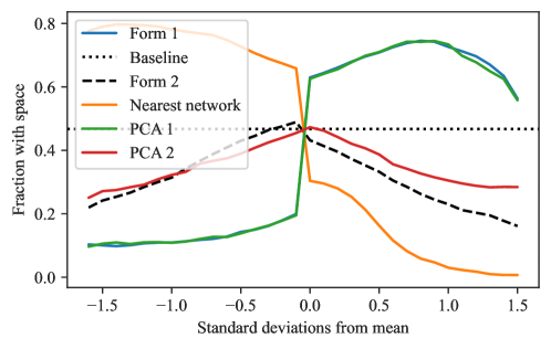
Figure 15: Analysis of Form $1$ in the language modeling setting. Among logit outputs for a token-in-context that are a given number of standard deviations away the mean, this shows the fraction of the form $[A][B]$ where $[B]$ begins with a space. The dotted line shows baseline probability of a token-in-context to be of this form. The “nearest network” is the neural network function at the timestep noted for Form $1$. Note the similarity of Form $\alpha$ to PC $\alpha$ for $\alpha\in\{1,2\}$. For the $\alpha=1$ pair many large positive logits fit the pattern $[A][B]$ where $[B]$ begins with a space, and large negative logits fit to $[A][B]$ where $[B]$ does not begin with a space. The $\alpha=2$ pair has a different mode of variation: many of its large positive and negative logits have $[B]$ begin with a space.

Form 2 ($t=17.7k$).

To interpret this form we examine extreme logits. As we show in Figure 16 the function $f^{*}_{2}$ assigns extreme logits (both positive and negative) to patterns of a form identified by Elhage et al. (2021) which we term here Induction Patterns (IPs). These are tokens-in-context of the form

$$\underline{\underline{[A]}}[B]\ldots\underline{[A]}[B]$$

where the token-in-context is the second occurrence of $[A]$ (the first being marked with two underlines) so the next token is $[B]$, repeating a pattern observed earlier in the context. The difference in the positions of the two occurrences of $[A]$ is what we call the search distance. Here are some examples of tokens-in-context assigned logits more than $1.5$ standard deviations above the mean, which contain IPs (we mark the search distance at the end of each example):

• / Euro/p/a/./ / /J/P/L/ built/ /and/ man/aged/ N/AS/A/’s/ G/al/ile/o/ mission/ for/ /the/ /ag/ency/’s/ S/cience/ M/ission/ Direct/or/ate/ in/ Washington/,/ /and/ is/ develop/ing/ /a/ concept/ for/ /a/ future/ mission/ /to/ Euro/p/ [distance 56]

• / d/iving/ exp/ed/ition/ in/ /the/ wat/ers/ of/ Br/une/i/ D/ar/uss/al/am/./ / /On/ his/ imp/ress/ions/ of/ his/ first/-/time/ d/iving/ [distance 32]

Examples more than $1.5$ standard deviations below the mean are unusual: the first five in our chosen set of tokens-in-context are instances where $[A],[B]$ are both the Unicode replacement character.

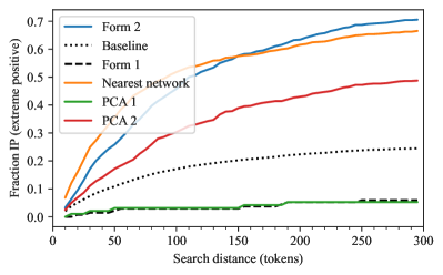
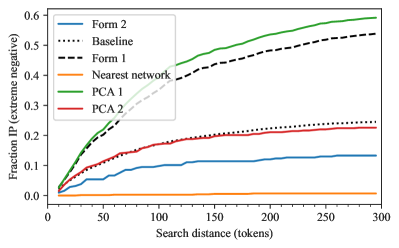
Figure 16: Analysis of Form $2$ in the language modeling setting. Left. Among logit outputs for a token-in-context that are more than $1.5$ standard deviations above the mean, shows the fraction which are IPs within the given search distance. Dashed line shows baseline probability of a token-in-context to be of this form. Right. Among logit outputs for a token-in-context that are $1.5$ standard deviations below the mean, shows the fraction which are IPs. The “nearest network” is the neural network function at the timestep noted for Form $2$. Note that these metrics distinguish Form $2$ from PC $2$.

C.2 Behavioral Development

C.2.1 Bigram Score

We empirically estimate the conditional bigram distribution by counting instances of bigrams over the training data. From this, we obtain the conditional distribution $\tilde{q}(t^{\prime}|t)$, the likelihood that a token $t^{\prime}$ follows $t$.

The bigram score $B_{k}^{S}$ at index $k$ of an input context $S$ is the cross entropy between the model’s predictions $p(t_{k+1}|t_{k})$ at that position and the empirical bigram distribution,

$$B_{k}^{S}=-\sum_{i=1}^{d_{\textrm{vocab}}}\tilde{q}(t_{k+1}^{(i)}|t_{k})\log p(t_{k+1}^{(i)}|t_{k}),$$ (31)

where the $t_{k+1}^{(i)}$ range over the possible second tokens from the tokenizer vocabulary. From this we obtain the average bigram score

$$\bar{B}=\frac{1}{n}\sum_{i=1}^{n}B_{k_{i}}^{S_{i}},$$ (32)

where we take fixed random sequences of $k_{i}$ and $S_{i}$ for $1\leq i\leq n=5,000$, which is displayed over training in Figure 3. This is compared against the best-achievable bigram score, which is the bigram distribution entropy itself, averaged over the validation set.

C.2.2 $n$-Gram Scores

In stage LM2 we consider $n$-grams, which are sequences of $n$ consecutive tokens, meaning $2$-grams and bigrams are the same. Specifically, we consider common $n$-grams, which is defined heuristically by comparing our 5,000 vocab size tokenizer with the full GPT-2 tokenizer. We use the GPT-2 tokenizer as our heuristic because its vocabulary is constructed iteratively by merging the most frequent pairs of tokens.

We first tokenize the tokens in the full GPT-2 vocabulary to get a list of 50,257 $n$-grams for various $n$. The first 5,000 such $n$-grams are all $1$-grams, after which $2$-grams begin appearing, then $3$-grams, $4$-grams, and so on (where $2$-grams and $3$-grams may still continue to appear later in the vocabulary). We then define the set of common $n$-grams as the first 1,000 $n$-grams that appear in this list for a fixed $n$, $n\geq 2$.

If we track the performance on $n$-grams and see it improve, we may ask whether this is simply a function of the model learning to use more context in general, rather than specifically improving on the set of $n$-grams being tracked. We measure performance against this baseline by defining an $n$-gram score. For a fixed $n$, we obtain the average loss $\ell_{\textrm{gram}}^{n}$ of the model on predicting the final tokens of our set of 1,000 $n$-grams and also obtain the average loss $\ell_{\textrm{test}}^{n}$ of the model on a validation set at position $n$ of each validation sequence. The $n$-gram score is then defined to be $\ell_{\textrm{test}}^{n}/\ell_{\textrm{gram}}^{n}$.

C.2.3 In-Context Learning Score

The in-context learning score is a behavioral measure of the relative performance of a model later in a sequence versus earlier in the sequence. We follow a similar construction as Olsson et al. (2022), where we take the loss at the 500th token minus the loss at the 50th token, so that a more negative score indicates better performance later in the sequence. This is then averaged over a 100k-row validation dataset. The performance of the language model over the course of training can be seen at the bottom of Figure 4.

C.2.4 Visualizing Behavioral Changes

In Figure 17, we visualize changes in the model’s input-output behavior by comparing model predictions before and after developmental stages and highlighting tokens with the greatest degree of differences.

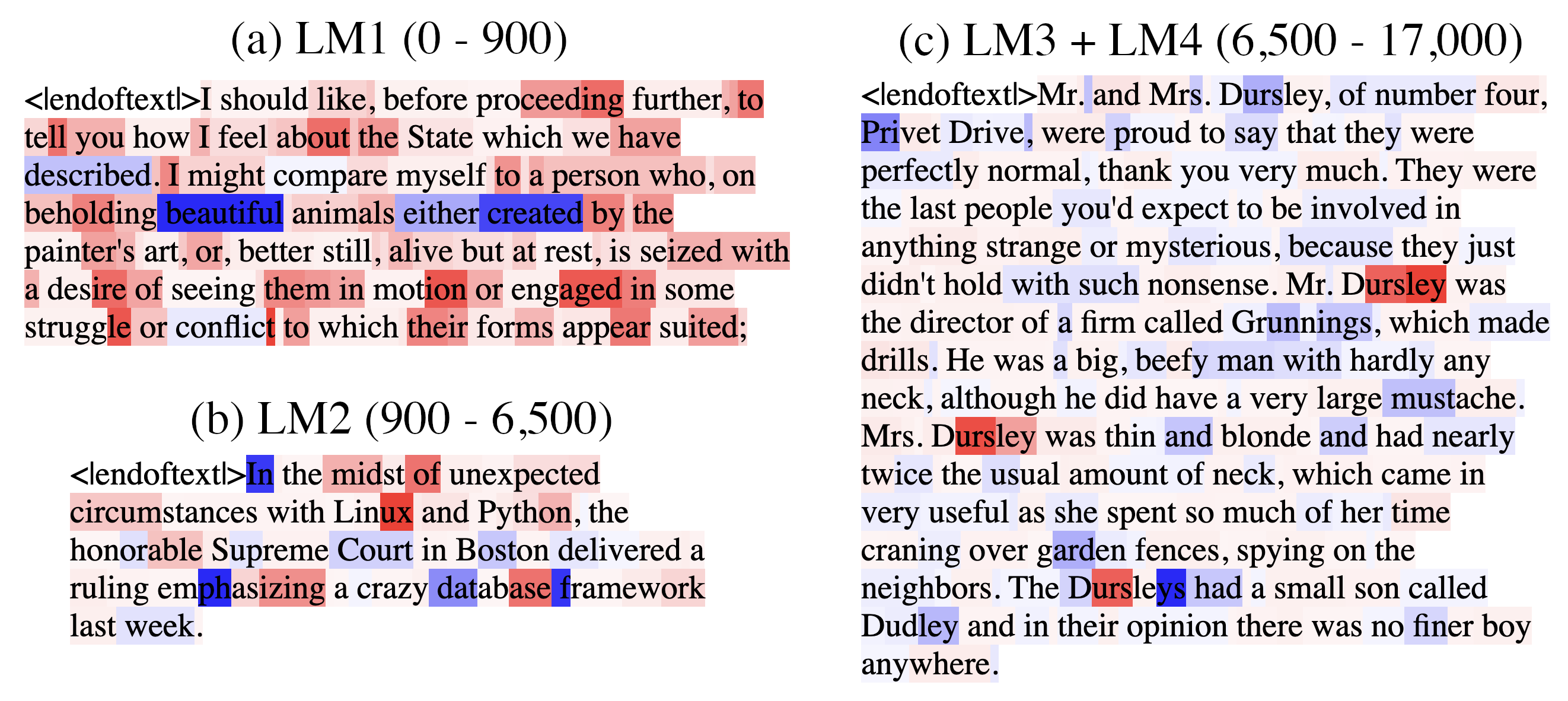
Figure 17: Sample texts are shown with tokens highlighted to indicate changes in model logit output from an earlier training checkpoint to a later one. Red indicates improved performance (higher logit output for the true next token) and blue indicates worse performance. Sample (a) corresponds to LM1, in which the model improves on bigrams, which is most visible in words like “te/ll, ab/out, des/ire, mot/ion, eng/aged, strugg/le, etc.” Sample (b) corresponds to improvement in common $n$-grams in LM2 such as “L/in/ux, P/y/th/on, h/on/or/able, S/up/reme, dat/ab/ase, f/ram/ew/ork.” Sample (c) represents the behavioral changes in LM3 and LM4, where the primary behavioral feature is the development of in-context learning via induction circuits. This is visible in the improved predictions in the word “D/urs/ley” after the first time it appears in the context, as initially observed by (Olsson et al., 2022).

C.3 Structural Development

C.3.1 Positional embedding

In Figure 18, we measure the effect of the positional embedding on model performance by comparing the model’s performance at particular context positions on a validation set over the course of training against performance on the same validation set but with the positional embedding zero-ablated. The full context length is 1024, and we measure test loss at positions 1, 2, 3, 5, 10, 20, 30, 50, 100, 200, 300, 500, and 1000. In the transition from stage LM1 to LM2, the model begins using the learnable positional embedding to improve performance. The difference between test loss with and without the positional ablation is negligible at all measured positions until the LM1–LM2 boundary.

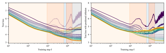
Figure 18: The model learns to start using the positional encoding in LM2, when the performance starts to worsen when ablating the positional encoding. In both plots, earlier token positions are colored more purple, while later token positions are more yellow, and the overall mean loss is colored in red. Both sets of per-token losses are shown in both graphs for ease of comparison. Left: original test loss is emphasized. Right: test loss with the positional embedding ablated is emphasized.

Structurally, we might predict that the positional embeddings should organize themselves in a particular way: in order to understand relative positions, adjacent positions should be embedded close to each other, and far-away positions should be embedded far apart.

In Figure 19, we examine the development of the positional embedding itself over time from two angles. The first is to take the embeddings of each position in the context and to run PCA on those embeddings. The result is that as training progresses, the positional embedding PCAs gradually resolve into Lissajous curves, suggesting that the positional embeddings look like a random walk (see Section B.7 for more details). However, if we look to the explained variance, we see that it grows very large for PC1, reaching $94.2\%$ at training step 6400. This is much higher than we would expect for Brownian motion, where we expect to see about $61\%$ explained variance in PC1 (Antognini & Sohl-Dickstein, 2018).

The second perspective we use is to look at how the magnitudes of positional embeddings over the context length develop. In this case, we observe that the magnitudes seem to have a fairly regular structure. In conjunction with the PCAs and explained variance, we might infer that the positional embeddings look approximately like a (possibly curved) line in $d_{\textrm{model}}=256$ dimensional space. A positional embedding organized in this way would make it easier for an attention head to attend to multiple recent tokens, which is necessary if a single head is to learn $n$-grams.

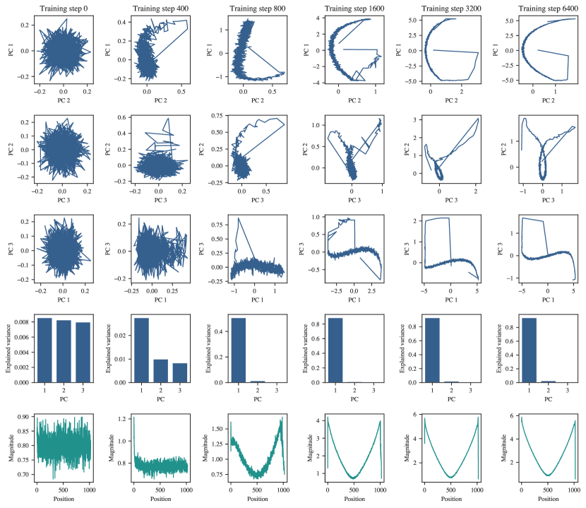
Figure 19: Columns progress through training time at training steps 0, 400, 800, 1600, 3200, and 6400. The first three rows are plots of the first three principle components of a PCA on the positional embedding weights, while the fourth row shows the explained variance for each of the principal components. The fifth row plots the magnitude of the embedding of each position in the context length of 1024.

C.3.2 Composition Scores

Let $W_{Q}^{h},W_{K}^{h},W_{V}^{h}$ be the query, key, and value weights of attention head $h$ respectively. There are three types of composition between attention heads in transformer models in Elhage et al. (2021):

• Q-Composition: the query matrix $W_{Q}^{h}$ of an attention head reads in a subspace affected by a previous head

• K-Composition: the key matrix $W_{K}^{h}$ of an attention head reads in a subspace affected by a previous head

• V-Composition: the value matrix $W_{V}^{h}$ of an attention head reads in a subspace affected by a previous head

If $W_{O}^{h}$ is the output matrix of an attention head, then $W_{QK}^{h}=W_{Q}^{h\ T}W_{K}^{h}$ and $W_{OV}^{h}=W_{O}^{h}W_{V}^{h}$. The composition scores are

$$||MW_{OV}^{h1}||_{F}/(||M||_{F}||W_{OV}^{h_{1}}||_{F})$$ (33)

Where $M=W_{QK}^{h_{2}\ T}$, $M=W_{QK}^{h_{2}}$, and $M=W_{OV}^{h_{2}}$ for Q-, K-, and V-Composition respectively. See Figure 20 for K-composition scores over time between attention heads in the induction circuits.

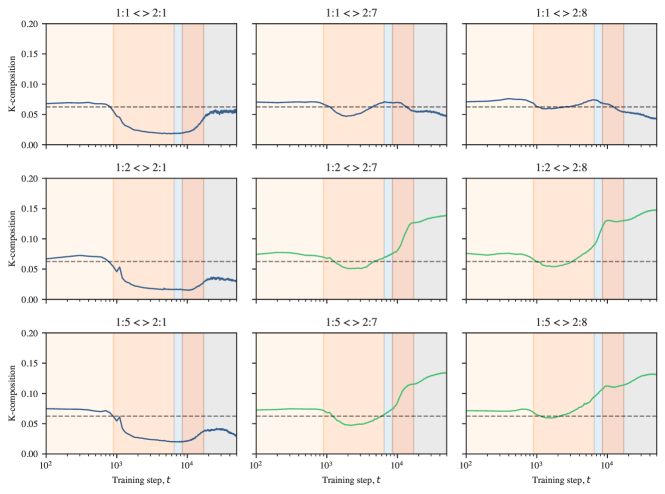
Figure 20: The K-composition scores Elhage et al. (2021) between first and second layer attention heads. The $h$th attention head in layer $l$ is indexed by $l:h$. The attention heads that eventually become previous token heads are $h=2,5$ in layer 1 (subplot rows 2 and 3), and the attention heads that eventually become induction heads are $h=7,8$ in layer 2 (subplot columns 2 and 3). The attention heads $1:1$ and $2:1$ are included for comparison. The induction heads $2:7$ and $2:8$ begin K-composing with first layer heads near the start of stage LM2. They continue to compose with the previous token heads in stages LM3 and LM4 (highlighted in green) while their K-composition scores drop with other attention heads in layer 1 in later stages.

C.3.3 Previous-Token Matching Score

The previous-token matching score is a structural measure of induction head attention. It is the attention score given to $[A]$ by an attention head at $[B]$ in the sequence $\ldots[A][B]$ (i.e., how much the head attends to the immediately preceding token).

We compute this score using a synthetic data generating process, generating 10k fixed random sequences with length between 16 and 64. The first token is a special “beginning of string” token, and the remaining tokens are uniformly randomly sampled from other tokens in the vocabulary.

For each sample in this synthetic data set, we measure the attention score that an attention head gives to the previous token when at the last token in the sequence. These scores are averaged across the dataset to produce the previous-token matching score for that attention head at a given checkpoint. The progression of previous-token matching scores over time can be seen in Figure 4.

C.3.4 Prefix Matching Score

The prefix matching score from Olsson et al. (2022) is defined similarly to the previous-token matching score. Given a sequence $[A][B]\ldots[A]$, the prefix matching score of a particular attention head is how much the attention head attends back to the first instance of $[A]$ when at the second instance of $[A]$.

We compute this score using a synthetic data-generating process. We first generate 10k fixed random sequences of length 128. The first token is always a special “beginning of string” token and the $[A]$ and $[B]$ tokens are selected and placed randomly. One $[A]$ token is placed in the first half of the sequence, the other is placed in the second half, and the $[B]$ token is placed directly after the first $[A]$ token. The remaining tokens are randomly sampled from the tokenizer vocabulary, excluding the $[A]$, $[B]$, and beginning of string tokens.

For each sample in this synthetic dataset, we measure the attention score that each attention head assigns to the earlier instance of $[A]$ from the latter instance of $[A]$. These scores are averaged across the dataset to produce the prefix matching score for that attention head at a given checkpoint. The progression of prefix matching scores over time can be seen in Figure 4.

C.4 One-layer Model Results

We also trained and ran some experiments on a one-layer language model (see Section E.1.1 for details). We aggregate results for the one-layer language model here, mirroring the experiments for the two-layer language model where possible. The early development of the one-layer model has many parallels with the two-layer model. At a single stage boundary, just as it occurs in the two-layer model, the one-layer model minimizes its bigram score (see Section C.2.1), begins utilizing the positional embedding to noticeably improve performance (see Section C.3.1), and starts making sudden improvements to the same $n$-gram scores (see Section C.2.2). Remarkably this occurs at the same checkpoint as in the 2-layer model (at 900 training steps).

One key difference, however, is that this occurs at the second stage boundary as discerned by the plateaus of the LLC estimation. We did not closely investigate why the LLC estimation appears to drop between steps 400 and 900 in this model. As a result though, we do observe an interesting qualitative similarity to the drop in LLC in stage LM3 of the two-layer model, that this drop precedes a noticeable bump in the loss function.

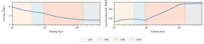
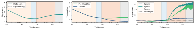
Figure 21: We train a one-layer transformer model in the language setting to compare with the two-layer model. The development of certain behavioral and structural indicators over time closely mirrors the development of the same indicators in the early stages of the two-layer language model. Top: test loss and LLC estimations over time for the one-layer attention-only transformer, compare with Figure 1(a). Bottom: bigram score, test loss with positional embedding ablated, and $n$-gram scores for the one-layer attention-only transformer, compare with Figure 3.

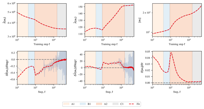
Figure 22: A more detailed version of Figure 21 for the one-layer language model. Top: Loss, LLC, and weight norm, along with an overlaid Gaussian process fit to these curves (red dotted lines). Bottom: Associated slopes, both numerically estimated finite differences (transparent blue) and of the Gaussian process (red dotted lined).

Appendix D Developmental Analysis of Regression Transformers

In this section, we present further evidence on the geometric (Section D.1), behavioral (Section D.2), and structural (Section D.3) development of the linear regression transformer (seed=1) over the course of training. In particular, we contrast the use of LLC with Hessian-derived statistics in Section D.1.3, and we analyze possible additional substages revealed by relaxing the stage identification criteria in Section D.1.4.

D.1 Geometric Development

D.1.1 LLC

Figure 23 displays the test loss and LLC curves from Figure 1(b) in addition to the weight norm over time, and numerically estimated slopes associated to these three metrics. As in the case of language models, we identify stage boundaries by looking for plateaus in the local learning coefficient. Unlike the language models, here the boundaries LR1–LR2 and LR2–LR3 are visible from the loss. However, LLC suggests additional substages (Section D.1.4) in LR3 that are invisible from the test loss.

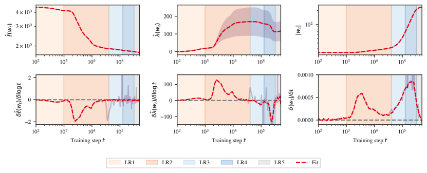
Figure 23: A more detailed version of Figure 1(b) for linear regression. Top: Loss, LLC, and weight norm, along with an overlaid Gaussian process fit to these curves (red dotted lines). Bottom: Associated slopes, both numerically estimated finite differences (transparent blue) and of the Gaussian process (red dotted lined). Top middle: Error bars displaying the standard deviation over the 10 SGLD chains are displayed in the background. Note that large error bars across chains are to be expected. Between different SGLD estimations, the variance is much lower. For example, averaged over training, the standard deviation over different seeds is only 4.2.

D.1.2 Essential Dynamics

Table 4: Forms for Regression Transformer.

Form	Vertex	Influence range	Content	PCs
1	2.5k	1.8k-2.6k	-	-
2	34.5k	30k-40k	-	$343,-65,45$
3	106.1k	90k-125k	-	$61,38,21$
4	168.9k	150k-190k	-	$-54,63,0$

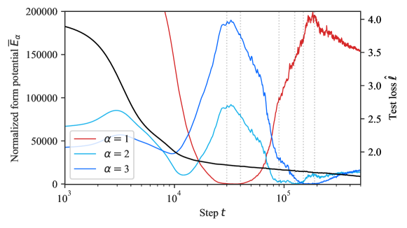
Figure 24: Normalized form potentials $\overline{E}_{\alpha}=E_{\alpha}-\inf_{t}E_{\alpha}(t)$ in the linear regression setting. The flat bottom of the potential corresponds to the period in which the developmental trajectory moves in a circular orbit around the associated form $f^{*}_{\alpha}$. Here, we plot three of the four form potentials; the first potential would occur at the far left of this figure.

Following the algorithm sketched in Section 3.2.1 and made more precise in Section B.3 we identify four forms of the developmental trajectory for the regression transformer, the details of which are shown in Table 4. The process of locating the evolute cusps and constructing the values in this table are shown in Figure 13. The associated form potentials are shown in Figure 24. We do not analyze the evolute or forms for LR5.

D.1.3 Hessians

Figure 25 shows the curvature-based notion of flatness captured by the Hessian (in contrast to the degeneracy-based notion of flatness captured by LLC). To estimate the trace and maximum eigenvalues shown in this figure, we use the PyHessian library Yao et al. (2020) over a batch of $m=1024$ samples.

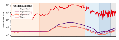
Figure 25: Hessian-based statistics correlate with stages but reveal only two of the four boundaries (Sections D.1.3 and D.1.4).

Crucially, we observe that these Hessian-derived metrics (henceforth, “curvature”) and the LLC are not consistently correlated. During the first part of LR2, the LLC and the curvature are jointly increasing. Starting at around $t=20\mathrm{k}$, while the LLC is still increasing, the curvature starts decreasing. In the first part of LR3, both metrics decrease in tandem, but as of around $t=120\mathrm{k}$, the curvature turns around and starts increasing.

While the Hessian provides further evidence for possible substage boundaries (Section D.1.4), it fails to detect two of the four macroscopic stage boundaries. Since these Hessian-based metrics are dominated by the largest eigenvalues — the directions of maximum curvature — they fail to observe the finer-grained measures of degeneracy that dominate the LLC. Moreover, we observe that LLC estimation is more scalable (empirically, it seems to be roughly linear in parameter count) than estimating the full Hessian (quadratic).

D.1.4 Additional Stages

Table 5: Possible substages for regression transformers. Including near-plateaus in the LLC curves and forms from ED suggest additional substages (Section D.1.4). Embedding collapse is depicted in Figure 29. Attention collapse is visible in Figure 32. Layer norm collapse is visible in Figures 30 and 31. ICL scores are shown in Figure 27.

Stage	End	LLC	Forms (Influence)	Behavior	Structure
LR1	1k	Plateau	2.5k (1.8k-2.6k)	Task prior learned	-
LR2a	7.5k	Near plateau	-	ICL emerges	-
LR2b	23k	Near plateau	34.5k (30k-40k)	$\operatorname{ICL}_{1:4}\downarrow,\operatorname{ICL}_{4:8}\approx$	Embedding & attn. collapse begin
LR2c	40k	Plateau	-	-	Layer norm (LN) collapse begins
LR3a	80k	Near plateau	-	“Overfitting” begins	-
LR3b	126k	Plateau	106.1k (90k-125k)	“Overfitting” continues	First LN weights reach 0
LR4a	220k	Near plateau	168.9k (150k-190k)	“Overfitting” continues	LN collapse beyond unembed
LR4b	320k	Near plateau	-	“Overfitting” finishes	LN collapse finishes
LR5	500k	Plateau	-	Convergence	-

Identifying boundaries with the LLC between stages of the same type requires specifying a threshold for the numerically estimated slope, below which we consider the model to be at an effective plateau (Section A.5). Relaxing this threshold to include “near-plateaus” can lead to new candidate stage boundaries. In the case of the linear regression models, this relaxation introduces candidate (sub)stage boundaries within LR2 at 7.5k steps and 23k, within LR3 at 80k and within LR4 at 220k steps.

The ED corroborates some of these additional substages (Table 4). In particular, the developmental trajectory is in the range of influence of the first form for steps 1.8k-2.6k, which would fall under LR2a, while the trajectory is in the range of influence of the second form between steps 30k-40k, which would fall under LR2c. The third form has its range of influence occurring in LR3b (90k-125k), and the fourth form has its range of influence occurring in LR4a (150k-190k).

These additional possible substages, and the evidence for them are detailed in Table 5.

The Hessian (Section D.1.3) provides further evidence for a boundary at around 20k steps and at around 120k steps, where we observe plateaus in the trace and maximum eigenvalues.

D.2 Behavioral Development

D.2.1 Task Prior Score

In addition to training models on a data distribution in which tasks $\task$ are generated on-the-fly, we examine the “discrete-task” setting of Raventós et al. (2023), in which a finite set of $M$ tasks is generated ahead of time, and training samples involve randomly selected tasks from this set.

Figure 26 depicts (a) the mean square distance between the model’s predictions and the zero prediction in addition to (b) the mean square distance between the model’s predictions and the “task prior” prediction, using the component-wise averaged $\overline{\task}$ over the set of tasks encountered during training. For all models, the minimum distance to the task prior prediction is lower than the minimum distance to the zero prediction. Hence, we call stage LR1 “learning the task prior” rather than simply learning the zero prediction.

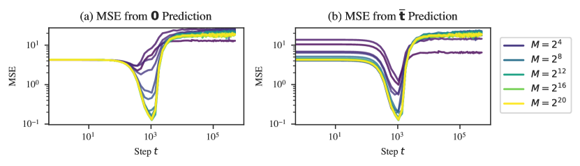
Figure 26: Learning the task prior is universal across models trained on very different data distributions. Each line represents a model trained on a data distribution with a different number of $M$ distinct tasks (“task diversity” in Raventós et al. (2023)). In addition to taking a finite $M$, the models depicted here differ from the other models considered in this paper in that the former were trained with a maximum learning rate of $0.01$, and the models (inadvertently) lack an output matrix after the multi-head attention layer.

D.2.2 ICL

We consider two variants of the ICL score 2: $\operatorname{ICL}_{1:D}$, and $\operatorname{ICL}_{D:K}$.

If the noise term $\sigma^{2}$ equals zero and both tasks $\task$ and inputs $x_{k}$ are normalized (i.e., $\task\in S^{D-1}$), then $D-1$ observations of input-output pairs are enough to precisely identify $\task$. Therefore, $I_{1:D}$ measures how successful the model is at initially locating the task. The fact that the tasks and inputs are not normalized changes this only slightly: the task will still sit near $S^{D-1}$ within a shell of vanishing thickness as $D\to\infty$.

Once localized, $I_{D:K}$ measures how successfully the model refines its internal estimate of $\task$ with additional examples, which it can use to reduce the error due to noise.

In terms of implementation, it’s not necessary for the model to internally make a distinction between locating and refining its estimate of the task. For example, ridge regression makes no distinction. Still, we find it useful for reasoning about the progression of the model. In particular, we note that early in stage LR2, while the model begins to develop ICL for early tokens, it becomes worse at ICL over tokens late in the context. Later, at around 23k steps, $\operatorname{ICL}_{D:K}$ stabilizes, while $\operatorname{ICL}_{1:D}$ continues improving over the entire training run.

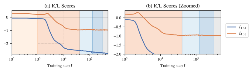
Figure 27: ICL scores for the linear regression model. Right: ICL scores between inputs 1 and 4 and inputs 4 and 8 over time. We see that ICL emerges during the first half of LR2. Left: Highlighted ICL score curves from the end of LR1 to halfway through LR2. Note that when the model first starts improving on early tokens, it temporarily becomes worse at predicting later tokens. Note also that the model ceases to become better at later tokens as of the second half of LR2, whereas ICL on early tokens continues to improve throughout training.

D.2.3 OOD Generalization

To further investigate behavior in stages LR2 and LR3, we probe the model on data sampled from different distributions than encountered during training. We evaluate behavior on two families of perturbations: “OOD inputs” $x_{k}$, sampled according to a different scale than encountered during training,

$$x_{k}\sim\mathcal{N}(0,gI_{D}),$$ (34)

for some gain parameter $g$, and “OOD tasks”

$$\task\sim\mathcal{N}(0,gI_{D}).$$ (35)

Note that these inputs/tasks are not out-of-distribution in the strong sense of coming from a distribution with a different support than the training distribution. However, the samples drawn from these “extreme” distributions are exponentially suppressed by the original training distribution and do not occur over any tractable number of training steps.

Plotting the MSE (normalized by dividing by $g^{2}$) for these two distributions over time reveals additional behaviorally distinct stages within LR2 and LR3 (Figure 28).

Between $t=1k$ and $t=4\mathrm{k}$ (roughly the proposed substage LR2a), the model’s outputs rapidly diminish in scale for out-of-distribution samples, both for $g>1$ and $g<1$, especially for out-of-distribution inputs. While the model is moving away from predicting with the task prior for in-distribution samples, it moves closer to predicting with the task prior for-in-distribution samples.

Between $t=4\mathrm{k}$ and $t=23\mathrm{k}$ (roughly the proposed substage LR2b), the model recovers on moderately out-of-distribution inputs $g<10^{1.5}$ with performance remaining close to constant beyond this range. Past this stage, performance improves constantly for out-of-distribution tasks.

For out-of-distribution inputs, performance eventually worsens for some ranges of $g$. During stages LR2c–LR3a (23k–80k), the model further approaches the task prior prediction for extreme out-of-distribution inputs $g>10^{1.5}$ . Subsequently, during LR3b and LR4c (75k–130k), the model moves away from the task prior prediction for extreme inputs, and performance deteriorates for inputs with $g>10^{0.5}$. As of LR5, performance is roughly constant.

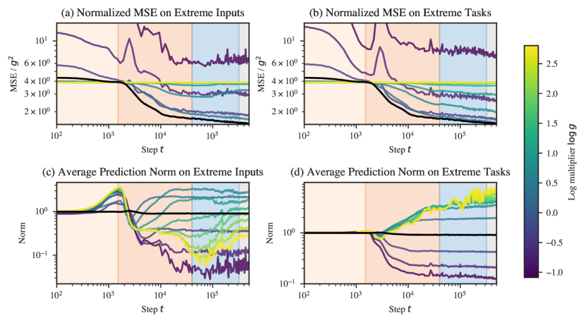
Figure 28: Performance on extreme inputs over time may reveal additional substages in LR2 and in LR3. Left: The model first becomes better, then worsens at ICL on inputs sampled from $\mathcal{N}(0,gI_{D})$ for large $g$. Right: The model continues to improve on ICL at tasks sampled from $\mathcal{N}(0,gI_{D})$. Top: Normalized loss (divided by $g^{2}$) over time for OOD inputs and tasks. Bottom: Average $|\hat{y}|$ over time for OOD inputs and tasks.

D.3 Structural Development

D.3.1 Embedding

The embedding matrix $W_{E}$ is a linear transformation from $\mathbb{R}^{D+1}\to\mathbb{R}^{{d_{\text{embed}}}}$. Plotting the $D+1$ singular values of this matrix, we notice that the embedding partially loses one of its components starting at the end of LR2 (Figure 29a).

The input “tokens” $x_{k}$ span a $D$-dimensional subspace of the $D+1$-dimensional “token space.” The target tokens $y_{k}$ span an orthogonal $1$-dimensional subspace. The collapse of one of the embedding matrix’s singular values means that the model learns to redundantly encode the inputs and targets in the same $D$-dimensional subspace of the space of residual stream activations. The almost order of magnitude separation in the magnitudes of the square singular value means that the $D+1$-th component of the token embedding explains only 2.9% of the variance in activations of the residual stream immediately after the embedding, whereas the dominant components explain roughly 24% each.

Contributions to degeneracy.

Given a linear transformation $T_{1}:\mathbb{R}^{D_{1}}\to\mathbb{R}^{D_{2}}$ followed by another linear transformation $T_{2}:\mathbb{R}^{D_{2}}\to\mathbb{R}^{D_{3}}$, reducing the rank of $T_{1}$ from $r$ to $r^{\prime}<r$ renders $D_{3}(r-r^{\prime})$ components of the second transformation irrelevant. This would mean a decrease in the learning coefficient of $D_{3}(r-r^{\prime})/2$ (a decrease in the effective dimensionality of $d$ leads to a decrease in the $d/2$ LLC). In the actual model, we don’t see an exact decrease in the rank, and a layer norm sits between the linear transformation of the embedding and the linear transformations of each transformer block and unembedding. It is unclear what the precise relation between structure and geometry is in this case (Section D.3.7). Still, suggestively, the onset of embedding collapse coincides with a decrease in the rate of increase of $\hat{\lambda}(w_{t})$.

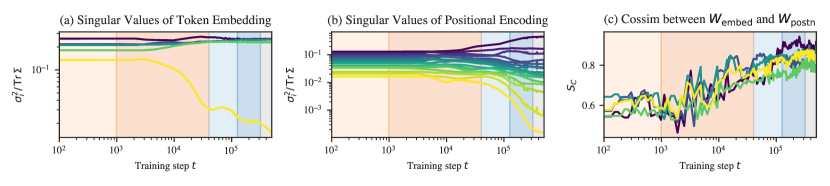
Figure 29: Left: The embedding partially “collapses” during the second half of LR2. At the start of stage LR2, the minimum singular values explains only 3% of the variance in residual stream activations due to the sample. By the end of training, it explains half that. Middle: The positional encoding goes through a similar shift during LR3 (that begins earlier during LR2). Right: The cosine similarity between the 5 rows of $W_{\text{embed}}$ and the projection of those rows onto the subspace spanned by $W_{\text{unembed}}$ shows that the model learns to write to the same write tokens and positional information to the same subspace.

D.3.2 Positional Encoding

The positional encoding goes through a similar collapse to the unembedding starting during the second part of LR2 and continuing into LR3 (Figure 29b). Additionally, throughout these stages, the subspace spanned by the embedding becomes more aligned with the subspace spanned by the positional encoding (Figure 29c).

Contributions to degeneracy.

For the same reason as with the token embedding, a decrease in the dimensionality of the subspace occupied by activations reduces the effective number of dimensions and thus the learning coefficient. This occurs both as the positional encoding’s effective dimensionality decreases (vanishing singular values, Figure 29b) and as the token embedding subspace and positional embedding subspace align (increasing cosine similarity, Figure 29b).

D.3.3 Unembedding Collapse

The unembedding block consists of a layer norm layer $\operatorname{LN}(z)$ followed by a linear transformation $W_{U}z+b_{U}$ and finally a projection $\pi_{y}$ to extract the $y$-component. Given the 64-dimensional vector of activations $z$ in the residual stream right before the unembedding (for a specific token), the full unembedding operation is:

$$\pi_{y}\left[W_{U}\cdot\left(\frac{z-\mathbb{E}[z]}{\sqrt{\mathbb{V}[z]+\epsilon}}*\gamma+\beta\right)+b_{U}\right].$$

Effective unembedding weights and biases.

Moving terms around, we can represent this as:

$$\left((W_{U})_{[0,:]}*\gamma\right)\cdot\left(\frac{z-\mathbb{E}[z]}{\sqrt{\mathbb{V}[z]+\epsilon}}\right)+\left((W_{U})_{[0,:]}\cdot\beta\right)+(b_{U})_{[0]}.$$

Because we are reading out a single $y$ component, we can express the unembedding transformation in terms of “effective” unembedding weights and biases:

$$\tilde{W}_{U}=(W_{U})_{[0,:]}*\gamma,$$

$$\tilde{b}_{U}=\left((W_{U})_{[0,:]}\cdot\beta\right)+(b_{U})_{[0]}.$$

Unembedding weights over time. In Figure 30, we plot $(\gamma,\beta)$, $((W_{U})_{[0,:]},(b_{U})_{[0]})$, and $(\tilde{W}_{U},\tilde{b}_{U})$ as a function of training steps, along with the mean weight over time. These are 64- and 1-dimensional vectors, so we can display the entire set of components. This reveals that the unembedding weights and biases are roughly constant and close to their initialization values until the end of LR3a. During stage LR3b, the majority of weights $\beta$ and $W_{U}$ “collapse” to zero. Additionally, the layer norm biases temporarily experience a large increase in variance before returning to small values. Despite this, the mean of the linear weights, layer norm biases, and effective weights remains remarkably constant and close to zero throughout the entire process.

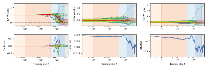
Figure 30: Unembedding weights over time for the $\lrt{1}$ transformer undergo a “collapse” that begins towards the end of LR2. When these weights reach zero in LR3 and LR4, it may contribute to the observed decrease in the LLC. Top: Weights over time. Bottom: Biases over time. Left: Unembedding layer norm weights over time. Middle: Unembedding linear weights over time (restricted to $y$-subspace). Right: Effective unembedding weights over time (obtained by element-wise multiplication of preceding columns, and focusing on the bias for only the $y$-token.

D.3.4 Layer Norm Collapse

The “collapse” in layer norm weights is not unique to the unembedding. As depicted in Figure 31, this behavior occurs in all layer norms except for the second MLP. The biases also remain centered close to zero even as the variance in biases grows much larger. Unlike in the unembedding, these layers begin to change earlier (starting in A2a).

What is most striking about the layer norm collapse is that it occurs without any explicit regularization (neither weight decay nor dropout). As such, it demonstrates a clear example of implicit regularization, i.e., inductive biases in the optimizer or model that favor simpler solutions.

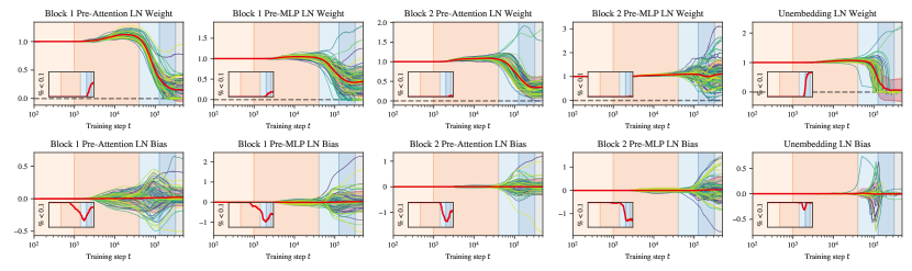
Figure 31: Layer norm weights over time. Top: After LR3, the layer norm collapse expands from the unembedding to earlier layers, most notably in the first pre-attention layer norm. This occurs without explicit regularization and may contribute to the concurrent decrease in LLC. Bottom: During layer norm collapse, the variance of layer norm biases increases drastically while the mean of the biases remains relatively constant. Inset: Plotting the fraction of weights or biases whose magnitude is less than 0.1 over time reveals that the collapse is more measured for intermediate layer norms: weights shrink to small values but not extremely close to zero as in the unembedding and first attention layer.

Contributions to degeneracy.

Given a layer norm $\operatorname{LN}:\mathbb{R}^{D_{1}}\to\mathbb{R}^{D_{1}}$ followed by a linear transformation $T:\mathbb{R}^{D_{1}}\to\mathbb{R}^{D_{2}}$ (as in the attention layers, MLPs, and unembedding), setting layer norm weights $\gamma_{i}$ to zero reduces the effective number of weights available in the linear transformation. If

$$T(x)=Wx+b,$$ (36)

and $\forall x:x_{i}=0$, then $\forall j:W_{ij}$ can be set to any arbitrary value without changing the output, so we expect $\lambda$ to decrease by $D_{2}/2$.

If $x_{i}$ is the output of a layer norm, then this holds if $\gamma_{i}=0$ for any choice of $\beta_{i}$. This follows from the fact that $\tilde{\beta}_{i}=W\beta$ is constant under the insertion of an invertible transformation $A$: $\tilde{\beta}_{i}=(WA^{-1})(A\beta)$.

D.3.5 Attention Collapse

Over the course of training, we observe that some attention heads learn to attend solely (soft attention becomes hard attention) and consistently to certain positions (the attention pattern becomes content-independent). We call this phenomenon attention collapse in parallel with the other observed forms of collapse. Not only does this potentially contribute to a decrease in the LLC, but it also makes the attention heads identifiable: we find a self-attention head, previous-attention heads, previous-$x$-attention heads, and previous-$y$-attention heads.

$x$-attention vs. $y$-attention.

For convenience we separate each attention head in two: one part for the $x$-tokens, and the other for the $y$-tokens.

Attention entropy score.

To quantify attention hardness, we use the attention entropy score Ghader & Monz (2017); Vig & Belinkov (2019). Given the attention pattern $\alpha_{k,k^{\prime}}^{(b,h)}$ for how much token $k$ in head $h$ in block $b$ attends back to token $k^{\prime}$, its attention entropy score $H_{k}^{(b,h)}$ is the Shannon entropy over preceding indices $k^{\prime}<k$,

$$H_{k}^{(b,h)}=-\sum_{k^{\prime}\leq k}\alpha_{k,k^{\prime}}^{(b,h)}\log_{2}\alpha_{k,k^{\prime}}^{(b,h)}.$$ (37)

From this, we compute the normalized entropy $\hat{H}_{k}^{(b,k)}$, which divides the attention entropy the maximum entropy for the given context length,

$$\hat{H}_{k}^{(b,h)}=\frac{H_{k}^{(b,h)}}{\log_{2}(k)}.$$ (38)

This accounts for the entropy being calculated over different numbers of tokens and is displayed in Figure 32. Notably, the identified stages line up closely to stages of these attention entropy curves.

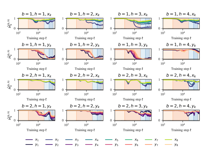
Figure 32: Attention hardening as measured by the normalized attention entropy score (Section D.3.5). Block 1 heads 1y/3y and block 2 head 1y harden over training. In combination with the fact that these attention heads become less variable (Figure 33), this may contribute to a decrease in the LLC (discussed in Section D.3.5) The x-components of the attention heads remain much softer over the entire training run.

Constant attention.

Accomplishing constant attention requires the presence of biases in the query and key transformations, or if there is no bias (as is the case for the models we investigated), requires attending to the positional embedding. With the Shortformer-style positional encoding used for the language models (Section E.1.1), this is straightforward: the positional information is injected directly into the key and weight matrices. With the linear regression models, where the positional embedding is added to the residual stream activations, this is less straightforward: achieving constant attention requires separating residual stream activations into orthogonal positional- and input-dependent subspaces, then reading from the former with the query and key weight matrices.

Attention variability score.

To quantify how constant the attention pattern is, we use measure attention variability Vig & Belinkov (2019),

$$V^{(b,h)}_{k}=\frac{\sum_{i=1}^{n}\sum_{k^{\prime}\leq k}\left|\alpha_{k,k^{\prime}}^{(b,h)}(S_{K}^{(i)})-\bar{\alpha}_{k,k^{\prime}}^{(b,h)}\right|}{2n\sum_{k^{\prime}\leq k}\bar{\alpha}_{k,k^{\prime}}^{(b,h)}},$$ (39)

where the division by $2$ ensures the variability lies in the range $[0,1]$. This is displayed in Figure 33. These reveal that though attention hardness and variability are independent axes of differentiation, empirically, we observe that hard attention is correlated with low variability.

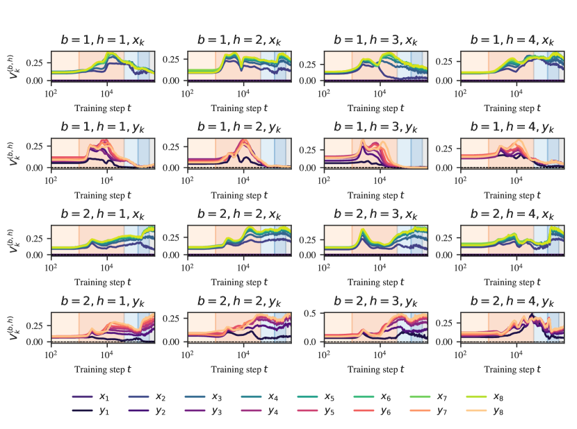
Figure 33: Attention variability over time. The heads that develop hard attention in Figure 32 (block 1 heads 1y, 3y, and 4y) also become less variable over time.

Contributions to degeneracy.

Suppose an attention head $h$ in block $b$ has the following constant attention pattern (after the softmax) $A^{(b,h)}=\sum_{i}\delta_{l(i)\,i}$. That is, for each token $i$, that attention head attends solely to a single earlier token $l(i)\leq i$ and no others. Restricting to single-head attention (the argument generalizes straightforwardly), the final contribution of this attention head to the residual stream is the following Phuong & Hutter (2022):

$$O=W_{O}\cdot(V\cdot A)$$ (40)

where $A\in\mathbb{R}^{\ell_{z}}\times\mathbb{R}^{\ell_{x}}$ is the attention pattern, $V\in\mathbb{R}^{d_{\text{out}}}\times\mathbb{R}^{\ell_{z}}$ is the value matrix, and $W_{O}\in\mathbb{R}^{d_{z}}\times\mathbb{R}^{\ell_{z}}$ is the matrix of residual stream activations, and $V\in\mathbb{R}^{d_{\text{out}}}\times\mathbb{R}^{\ell_{z}}$ is the value matrix. The result of this operation is subsequently multiplied by the output matrix and then added back into the residual stream. Plugging in the hard and constant attention pattern, writing out the matrix multiplication, and filling in the definition of $A$ we get

$$O_{ij}=\sum_{k}(W_{O})_{ik}V_{kl(j)}\delta_{l(j)j}.$$ (41)

For each column in $A$, the hard attention picks out a single element of $V$ at column $l(j)$ for each row $k$. Now suppose that there is a token $l^{\prime}$ that receives no attention from any position $j$. That is, there exists no $j$ such that $l^{\prime}=l(j)$. Then, there is a column $l^{\prime}$ in $V$ which does not contribute to the result of $V\cdot A$, and, in turn, a column $l^{\prime}$ in $W_{O}$, which does not contribute to the output of the head. As discussed for the embedding and layer norm, this decrease in effective dimensionality leads to a decrease in the learning coefficient.

Note that this argument does not hold for all hard and constant attention patterns. It holds solely for attention patterns that consistently ignore some earlier token across all positions, such as the previous-$x$ and previous-$y$ heads, but not the self-attention and previous-token heads. As discussed in Section D.3.7, it remains unclear what exactly the threshold for “ignoring” a token should be before it contributes to degeneracy and whether any of the heads we examine actually meet this threshold.

D.3.6 Classifying Attention Heads

Several attention heads are easy to identify by virtue of being both concentrated and consistent. These are depicted in Figure 34 and include: (B1H3y) previous-token heads (also present in the language model case), (B1H1y) previous-x, and (B1H4x, B2H1y) previous-y heads. Other training runs also include self-attention heads.

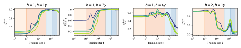
Figure 34: Collection of attention heads identified by their consistent and recognizable attention patterns. Left to right: previous-$x$s head, previous-token head, previous-$y$s head, previous-$y$s head

Self-attention score.

Self-attention is measured by the average amount a token $k$ attends to itself, $\alpha_{k,k}^{(b,h)}$.

Previous-token attention score.

Previous-token attention is measured the same as in the language model setting (Section C.3) with one difference: we compute the previous-token score not over a synthetic dataset but over a validation batch.

$x$-attention score.

The total amount attended to inputs $x_{k}$, that is $\alpha_{k,x}^{(b,h)}=\sum_{k^{\prime}=1}^{K}\alpha_{k,2k}^{(b,h)}$.

$y$-attention score.

Defined analogously $\alpha_{k,x}^{(b,h)}=\sum_{k^{\prime}=1}^{K}\alpha_{k,2k+1}^{(b,h)}$.

D.3.7 Increasing Degeneracy

Above we provided theoretical arguments for how embedding (Section D.3.1), layer norm (Section D.3.4), and attention collapse (Section D.3.5) can lead to an increase in degeneracy and thus a decrease in the LLC. These arguments hinge on the collapse being complete, that is, the components that go to zero must become exactly zero in the limit where we take the number of samples to compute the loss to infinity. In practice, we expect there to be some threshold $\epsilon$ below which we can treat weights as effectively zero.

Actually establishing a link between these particular phenomena and changes in the LLC is beyond the scope of this paper. We provide these analyses as a source of intuition for how structure and geometry can be related.

Appendix E Experimental Details

E.1 Language Models

E.1.1 Model

The language model architectures we consider are one- and two-layer attention-only transformers. They have a context length of 1024, a residual stream dimension of $d_{model}=256$, $H=8$ attention heads per layer, and include layer norm layers. We also used a learnable Shortformer positional embedding (Press et al., 2021). The resulting models have a total of $d=3,091,336$ parameters for $L=1$ and $d=3,355,016$ parameters for $L=2$. We used an implementation provided by TransformerLens (Nanda & Bloom, 2022).

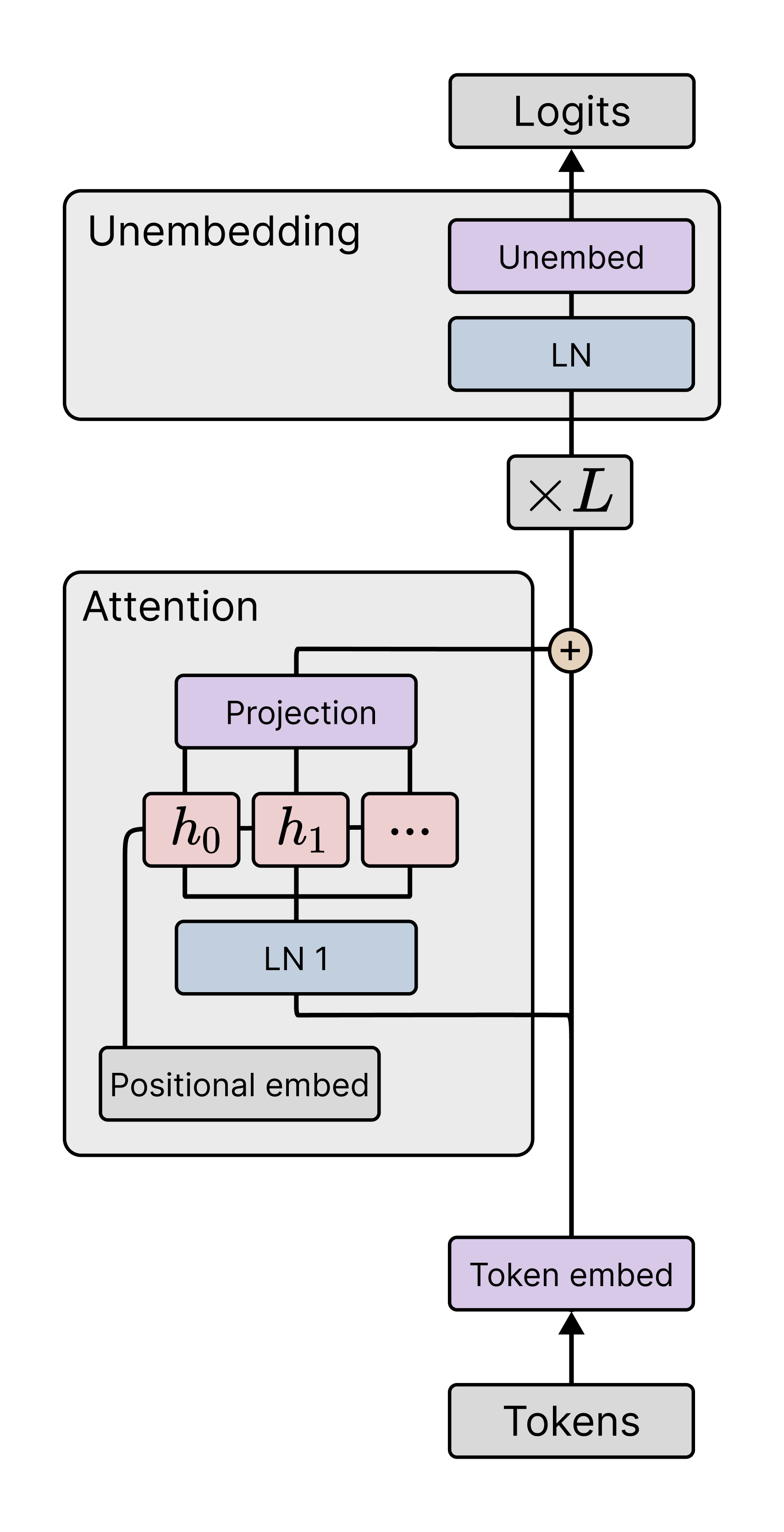
Component	1-Layer	2-Layer
Token Embedding Weights	$1,280,000$
Positional Embedding Weights	$262,144$
Layer 1 Layer Norm Weights	$256$
Layer 1 Layer Norm Bias	$256$
Layer 1 Attention Query Weights	$65,536$
Layer 1 Attention Key Weights	$65,536$
Layer 1 Attention Value Weights	$65,536$
Layer 1 Attention Output Weights	$65,536$
Layer 1 Attention Query Bias	$256$
Layer 1 Attention Key Bias	$256$
Layer 1 Attention Value Bias	$256$
Layer 1 Attention Output Bias	$256$
Layer 2 Layer Norm Weights	N/A	$256$
Layer 2 Layer Norm Bias	N/A	$256$
Layer 2 Attention Query Weights	N/A	$65,536$
Layer 2 Attention Key Weights	N/A	$65,536$
Layer 2 Attention Value Weights	N/A	$65,536$
Layer 2 Attention Output Weights	N/A	$65,536$
Layer 2 Attention Query Bias	N/A	$256$
Layer 2 Attention Key Bias	N/A	$256$
Layer 2 Attention Value Bias	N/A	$256$
Layer 2 Attention Output Bias	N/A	$256$
Final Layer Norm Weights	$256$
Final Layer Norm Bias	$256$
Unembedding Weights	$1,280,000$
Unembedding Bias	$5,000$

Figure 35: Attention-only transformers with Shortformer position-infused attention and pre-layer norm. The one-layer model has a total of 3,091,336 trainable parameters, while the two-layer model has 3,355,016.

E.1.2 Training

The models are trained on a single epoch over $50,000$ steps on $\sim$5 billion tokens using a resampled subset of the Pile (Gao et al., 2020; Xie et al., 2023) using a batch size of $100$. A snapshot was saved every $10$ steps for a total of $5000$ checkpoints, though a majority of analysis used checkpoints every 100 steps. The training time was around 6 GPU hours per model on an A100.

Training was conducted on the first 10 million lines of the DSIR-filtered Pile (Xie et al., 2023; Gao et al., 2020) but did not exhaust all 10 million lines. The model was subject to weight decay regularization, without the application of dropout. Additionally, we did not employ a learning rate scheduler throughout the training process.

Tokenizer.

For tokenization, we used a truncated variant of the GPT-2 tokenizer that cut the original vocabulary of 50,000 tokens down to 5,000 (Eldan & Li, 2023) to reduce the size of the model. We think this may contribute to the prominence of the the plateau at the end of LM1: the frequency of bigram statistics depends on your choice of tokens, and a larger tokenizer leads to bigrams that are individually much less frequent.

Table 6: Summary of Hyperparameters and Their Values for Both Language Model

Hyperparameter	Category	Description/Notes	Value
$n$	Data	Number of training samples	$10,000,000$
$T$	Data	Number of training steps	$50,000$
Tokenizer Type	Data	Type of Tokenizer	Truncated GPT-2 Tokenizer
$D$	Data	Vocabulary size	5,000
$K$	Data	Maximum in-context examples	1,024
$L$	Model	Number of layers in the model	$2$
$H$	Model	Number of attention heads per layer	8
$d_{\mathrm{mlp}}$	Model	Size of the hidden layer in MLP	N/A
$d_{\mathrm{embed}}$	Model	Embedding size	256
$d_{\text{head}}$	Model	Head size	32
$\mathrm{seed}$	Model	Model initialization	1
m	Training	Batch Size	100
Optimizer Type	Optimizer	Type of optimizer	AdamW
$\eta$	Optimizer	Learning rate	$0.001$
$\lambda_{\mathrm{wd}}$	Optimizer	Weight Decay	$0.05$
$\beta_{1,2}$	Optimizer	Betas	$(0.9,0.999)$

E.1.3 LLC estimation

For local learning coefficient estimation, we use SGLD to sample 20 independent chains with 200 steps per chain and 1 sample per step, at a temperature $\beta=1/\log(m)$, where $m=100$ is the size of the batch (the maximum size that would fit in memory). For the one-layer model, we used $\epsilon=0.003,\gamma=300$, and for the two-layer model we used $\epsilon=0.001,\gamma=100$. Estimating the local learning coefficient across all checkpoints took around 200 GPU hours for the two-layer model on a single A100 and around 125 GPU hours for the one-layer model.

For SGLD-based LLC estimation, we sampled a separate set of 1 million lines (lines 10m-11m) from the DSIR filtered Pile, denoted as $D_{\text{sgld}}$. The first 100,000 lines from this SGLD set (lines 10m-10.1m) were used as a validation set. The sampling of batches for SGLD mirrored the approach taken during the primary training phase. Each SGLD estimation pass was seeded analogously, so, at different checkpoints, the SGLD chains encounter the same selection of batches and injected Gaussian noise.

Table 7: Hyperparameters for Estimating the Local Learning Coefficient for Language Models.

Hyperparameter	Category	Description/Notes	1-Layer	2-Layer
C	Sampler	The number of chains	$20$
$T_{\mathrm{SGLD}}$	Sampler	The number of SGLD steps per chain	$200$
$\epsilon$	SGLD	The step size	$0.003$	$0.001$
$\gamma$	SGLD	The localization strength	$300$	$200$
$\beta$	SGLD	The inverse temperature, usually set to $\beta^{*}=\frac{1}{\log n}$	0.0000217147
$m$	SGLD	The size of each SGLD batch	100
$\mathcal{O}$	Data	Which dataset to use for evaluations. Either $L_{\mu}$, $L_{m^{\prime}}$, $\batchloss[(\tau^{\prime})]$, or $\batchloss[\tau]$	$L_{m}$
$D_{?}$	Data	Which dataset to sample batches from.	$D_{\text{sgld}}$
$\mu$	Data	The size of the dataset from which gradient minibatches are sampled	1m

E.1.4 Essential Dynamics

The functional proxy we use for behavioral essential dynamics (Section 3.2) is prepared as follows: we fix a sequence of training checkpoints $t_{1},\ldots,t_{T}$ and a set of $n=10,000$ randomly chosen output tokens, each from a different input sequence and context position. At each checkpoint $t_{i}$, we evaluate the logits $\ell_{j}^{i}$ at each of the tokens and construct a vector $v_{i}=(\ell_{1}^{i},\ldots,\ell_{n}^{i})$. We then apply PCA to the set $\{v_{i}\}_{i=1}^{T}$.

E.2 Regression Transformers

E.2.1 Model

In the following $L$ refers to the number of layers (blocks) in the Transformer, $H$ is the number of heads in each layer, $D$ is the dimension of inputs $x\in\mathbb{R}^{D}$ and $K$ is the number of $(x,y)$ pairs provided to the Transformer in-context.

The architecture is a pre-layer-norm decoder-only transformer modeled after NanoGPT Karpathy, 2022; see also Phuong & Hutter, 2022 with a learnable positional embedding. For the models discussed in the main body, we consider $L=2$, $H=4$ transformers (with $d=51,717$ parameters), i.e., two transformer blocks with four attention heads each.

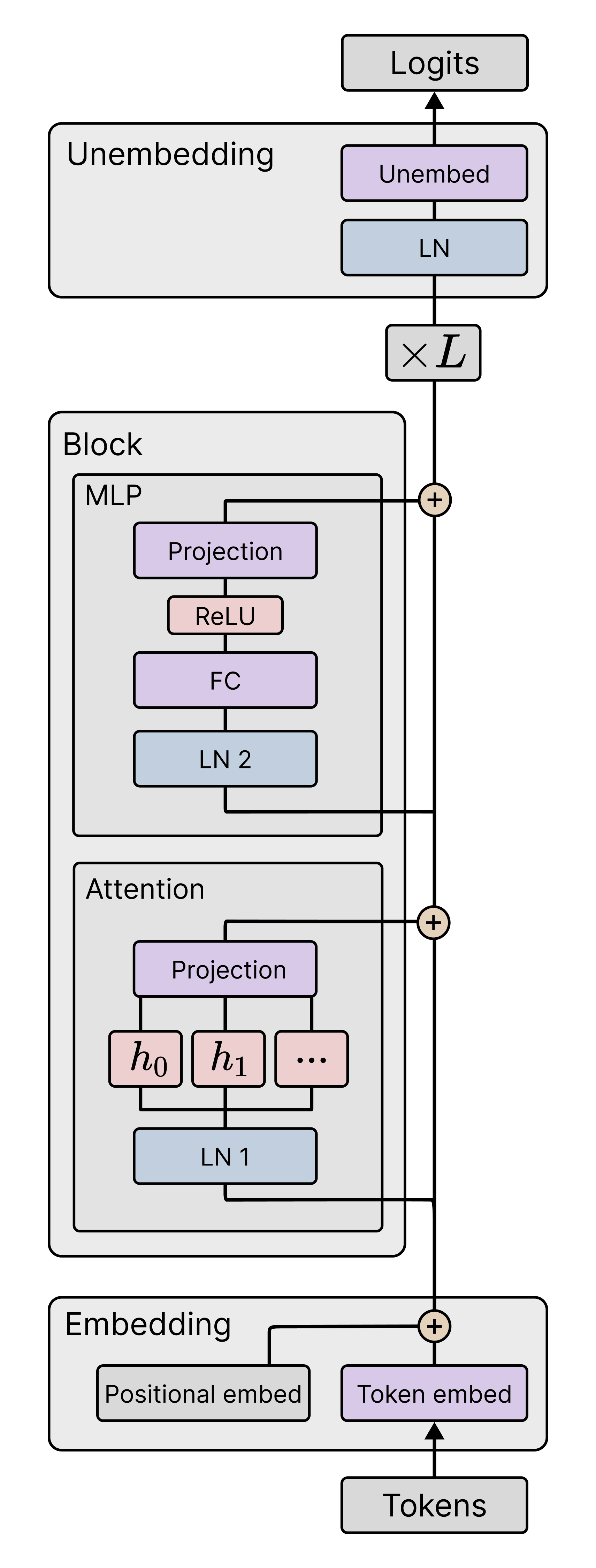
Component	Number of Parameters
Token Embedding Weight	$320$
Positional Embedding Weight	$1,024$
Layer 1 Layer Norm Weight 2	$64$
Layer 1 Layer Norm Bias 1	$64$
Layer 1 Attention Weights	$12,288$
Layer 1 Attention Output Weights	$4,096$
Layer 1 Layer Norm Weight 1	$64$
Layer 1 Layer Norm Bias 2	$64$
Layer 1 Feed-Forward MLP Weight	$4,096$
Layer 1 Feed-Forward MLP Bias	$64$
Layer 1 Feed-Forward Output Weight	$4,096$
Layer 1 Feed-Forward Output Bias	$64$
Layer 2 Layer Norm Weight 1	$64$
Layer 2 Layer Norm Bias 1	$64$
Layer 2 Attention Weights	$12,288$
Layer 2 Attention Output Weights	$4,096$
Layer 2 Layer Norm Weight 2	$64$
Layer 2 Layer Norm Bias 2	$64$
Layer 2 Feed-Forward MLP Weight	$4,096$
Layer 2 Feed-Forward MLP Bias	$64$
Layer 2 Feed-Forward Output Weight	$4,096$
Layer 2 Feed-Forward Output Bias	$64$
Unembedding Layer Norm Weight 1	$64$
Unembedding Layer Norm Bias 1	$64$
Unembedding Weight 2	$320$
Unembedding Bias 2	$5$

Figure 36: Transformer parameters in the linear regression setting. The model has two transformer blocks for a total of $51,717$ trainable parameters.

E.2.2 Tokenization

To run contexts $S_{K}$ through the above model requires an initial encoding or “tokenization step” and final “projection step.” The context is encoded as a sequence of “tokens” $T_{k}$ as follows:

$$T_{k}=\left(\begin{pmatrix}0\\ \vline\\ x_{1}\\ \vline\end{pmatrix},\begin{pmatrix}y_{1}\\ 0\\ \vdots\\ 0\end{pmatrix},\cdots\begin{pmatrix}0\\ \vline\\ x_{k}\\ \vline\end{pmatrix},\begin{pmatrix}y_{k}\\ 0\\ \vdots\\ 0\end{pmatrix}\right).$$

Through the main text, we write $f_{w}(S_{k})$ for $f_{w}(T_{k})$. Note that this tokenization includes the final $y_{k}$ token even though this receives no training signal. For this reason, we omit this token from the attention entropy and variability plots (Figures 32 and 33).

The transformer outputs a series of tokens of the same shape as $T_{k}$. To read out the $\hat{y}_{k}$ predictions, we read out the first component of every other token, i.e.,

$$\pi_{Y}:\mathbb{R}^{2K}\times\mathbb{R}^{D+1} \to\mathbb{R}^{K}$$ (42)

$$\left(\begin{pmatrix}\hat{y}_{1}\\ \vdots\\ \end{pmatrix},\begin{pmatrix}.\\ \vdots\end{pmatrix},\cdots,\begin{pmatrix}\hat{y}_{k}\\ \vdots\\ \end{pmatrix}\right) \mapsto(\hat{y}_{1},\dots,y_{k}).$$ (43)

E.2.3 Training

We train from a single seed for each choice of architecture and optimizer hyperparameters using minibatch stochastic gradient descent. We train without explicit regularization and use the Adam optimizer (Kingma & Ba, 2014). The training runs take 1 to 5 TPU-hours on TPUs provided by Google Research. Models are trained from the same initialization and on the data vectors within each batch (but for different sets of tasks and task orderings).

Models are trained on a single epoch: each of the $T=500,000$ batches consists of a new set of sequences with batch size 256. For the LLC estimates, we save 190 checkpoints: 100 are linearly spaced over the training run, and the remaining 90 are logarithmically spaced. We perform local learning coefficient estimation and other analyses on these checkpoints. For the essential dynamics, we take a larger set of 5,000 linearly spaced checkpoints from the same training run.

Table 8: Summary of Hyperparameters and Their Default Values

Hyperparameter	Category	Description/Notes	Default Values
$n$	Data	Number of training samples	128,000,000
$B$	Data	Batch size during training	256
$T$	Data	Number of training steps	500k
$D$	Data	Dimensions of linear regression task (Task size)	4
$K$	Data	Maximum in-context examples	8
$\sigma^{2}$	Data	Variance of noise in data generation	0.125
$L$	Model	Number of layers in the model	2
$H$	Model	Number of attention heads per layer	4
$d_{\mathrm{mlp}}$	Model	Size of the hidden layer in MLP	64
$d_{\mathrm{embed}}$	Model	Embedding size	64
$\mathrm{seed}$	Misc	Training run seeds	{0, 1, 2, 3, 4}
Optimizer Type	Optimizer	Type of optimizer	Adam
$\eta$	Optimizer	Maximum learning rate	0.003
$\lambda_{\mathrm{wd}}$	Optimizer	Weight Decay	0
$\beta_{1,2}$	Optimizer	Betas	(0.9, 0.999)
Scheduler Type	Scheduler	Type of learning rate scheduler	OneCycleLR
Strategy	Scheduler	Strategy for annealing the learning rate	Linear
% start	Scheduler	Percentage of the cycle when learning rate is increasing	0.5

E.2.4 LLC Estimation

For local learning coefficient estimation, we generate a fixed dataset of $2^{20}$ samples. Using SGLD, we sample $10$ independent chains with 5,000 steps per chain, of which the first 1,000 are discarded as a burn-in, after which we draw observations once per step, at a temperature $\epsilon\beta/2n=0.01$, $\epsilon=0.0003$, and $\epsilon\gamma/2=0.01$, over batches of size $m=1024$. Local learning coefficient estimation takes up to 72 CPU-hours per training run.

Table 9: LLC estimation hyperparameters. A summary of the hyperparameters involved in estimating the local learning coefficient and the default values we use.

Hyperparameter	Category	Description/Notes	Default Values
C	Sampler	The number of chains	$10$
$T_{\mathrm{SGLD}}$	Sampler	The number of SGLD steps per chain	$5,000$
$\epsilon$	SGLD	The step size	$0.0003$
$\tilde{\gamma}=\epsilon\gamma/2$	SGLD	The localization strength	$0.01$
$\tilde{\beta}=\epsilon\beta/2n$	SGLD	The inverse temperature, usually set to $\beta^{*}=\frac{1}{\log n}$	$0.01$
$m$	SGLD	The size of each SGLD batch	$2^{10}$
$\mathcal{O}$	Data	Which dataset to use for evaluations. Either $L_{\mu}$, $L_{m^{\prime}}$, $\batchloss[(\tau^{\prime})]$, or $\batchloss[\tau]$	$D_{\mathrm{val}}$
$\mu$	Data	The size of the dataset from which gradient minibatches are sampled	$2^{20}$

E.2.5 Essential Dynamics

The functional proxy we use for behavioral ED is defined as follows: we draw a fixed batch of $m=1024$ input sequences $\{S_{K}^{i}\}_{i=1}^{m}$ and observe the full model outputs $f_{w_{t}}(S^{i}_{K})\in\mathbb{R}^{2K(D+1)}$ over a set of 5000 linearly spaced checkpoints indexed by $t$. These are the outputs before the final projection step detailed in Section E.2.2 and include not only the scalar predictions $\hat{y}_{k}$ for each $x_{k}$ input but also the values of the $D$ other indices in the output “tokens” and the $K$ other output “tokens” for each $y_{k}$ input (which are not trained against). We stack these outputs to obtain the functional proxy $F_{w_{t}}=\{f_{w_{t}}(S^{i}_{K})\}_{i=1}^{m}\in\mathbb{R}^{2m(D+1)K}$ and apply PCA to the trajectory of this functional proxy over checkpoints. For the developmental trajectory of Figure 2 we pre-process the datapoints by smoothing with Gaussian kernel (standard deviation ranging from $15$ in LR1 to $60$ halfway through LR2) and we then compute osculating circles to this smoothed curve.

E.3 SGLD-Based LLC estimation

This section walks through some of the hyperparameter choices and sweeps involved in calibrating LLC estimates. We provide it as a reference for others seeking to adjust LLC estimation to novel settings.

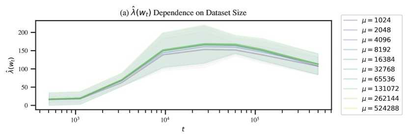
Figure 37: Past some threshold, the choice of validation set size from which SGLD batches are sampled has little effect on learning coefficient estimates. Estimation hyperparameters are $C=8,T_{\mathrm{SGLD}}=2,000,m=2^{10},\epsilon=0.0003,\tilde{\gamma}=0.01,\tilde{\beta}=0.01$. Loss is evaluated over gradient minibatches at a representative selection of checkpoints. LLCs quickly converge to a constant value as the size increases.

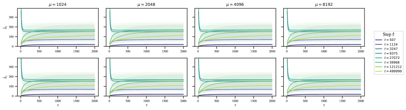
Figure 38: The size of SGLD minibatches has a negligible effect on LLC estimates (at least among the batch sizes considered). Top: Loss is evaluated on the same minibatch as the SGLD gradients. Bottom: Loss is evaluated on a newly sampled minibatch from the SGLD gradients (of the same size). Estimation hyperparameters are $C=8,T_{\mathrm{SGLD}}=2,000,\mu=2^{20}$.

E.3.1 Varying the temperature

In Lau et al. (2023), the inverse temperature is set to a fixed “optimal” temperature $\beta^{*}=1/\log n$.

The inverse temperature $\beta$ and the dataset size $n$ always show up together as product, both in 14 for the SGLD step and in the equation for the local learning coefficient,

$$\hat{\lambda}^{\beta}(w_{t})=\beta n\left(\mathbb{E}_{w|w_{t}}^{\beta}[\hat{\ell}(w)]-\hat{\ell}(w_{t})\right).$$ (44)

This allows us to view the inverse temperature $\beta$ as a dataset multiplier, that increases the effective size of your dataset. In a Bayesian context, $\beta=2$ would mean you update twice on each of the samples in your dataset.

For large $n$, using $\beta^{*}$ is suboptimal in SGLD. As we increase $n$, we have to decrease $\epsilon$ to prevent the SGLD step from becoming ill-conditioned. If $n$ is large enough, this leads to a problem where the injected noise term becomes entirely suppressed by the gradient term. This, in turn, leads to requiring larger batches to suppress the gradient noise and requiring longer chains to sufficiently explore the local posterior. Thus, for loss-based LLC estimation, we propose performing SGLD-based sampling above the Watanabe temperature (Section E.3.3).

E.3.2 Seeding the random noise

To smooth out the $\hat{\lambda}_{t}$ curves, we reset the random seed before LLC estimation run at each checkpoint. This means the sequence of injected Gaussian noise is the same for LLC estimation runs at different checkpoints. Additionally, if the batch size is held constant, the batch schedule will also be constant across different estimation runs. Figure 39 shows that this does not affect the overall shape of the learning coefficient curves; it simply smooths it out.

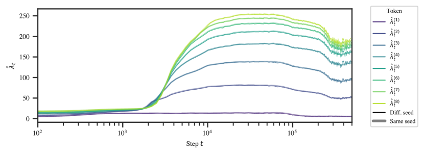
Figure 39: Consistently seeding SGLD estimates at each checkpoint smooths out the resulting LLC-over-time curve. Except towards the end of training (this is plotted over a log time axis), the difference is barely noticeable. Variable seeds yield a noisier set of estimates.

E.3.3 Calibrating $\epsilon$, $\beta$, and $\gamma$

As a rule of thumb, $\epsilon$ should be large enough that the $\hat{\lambda}$ estimate converges within the $T_{\mathrm{SGLD}}$ steps of each chain but not too large that you run into issues with numerical stability and divergent estimates. Subject to this constraint, $\gamma$ should be as small as possible to encourage exploration without enabling the chains to “escape” to nearby better optima, and $\beta$ should be as large as possible (but no greater than $1/\log n$).

To determine the optimal SGLD hyperparameters, we perform a grid sweep over a reparametrization of the SGLD steps in terms of $\tilde{\beta},\tilde{\gamma},\varepsilon$:

$$\Delta w_{t}=\tilde{\beta}\nabla L^{(\tau)}_{m}+\tilde{\gamma}(w^{*}-w_{t})+N(0,\varepsilon),$$

where $\tilde{\beta}=\varepsilon\beta n/2$, $\tilde{\gamma}=\varepsilon\gamma/2$.

The results of this hyperparameter sweep are illustrated in Figure 40 for final checkpoints. Separately (not pictured), we check the resulting hyperparameters for a subset of earlier checkpoints. This is needed since, for example, a well-behaved set of hyperparameters at the end of training may lead to failures like divergent estimates (Figure 41) earlier in training when the geometry is more complex and thus the chains less stable.

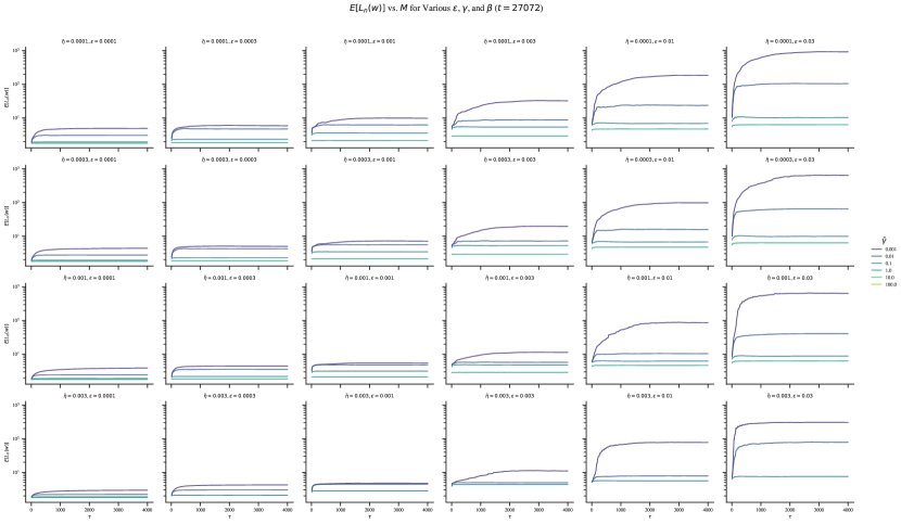
Figure 40: Results of grid sweep over SGLD hyperparameters for model 0 at $t=500\mathrm{k}$.

E.3.4 LLC traces

As a useful diagnostic when calibrating the local learning coefficient estimates, we propose an online variant for learning coefficient estimation. When overlaid on top of individual-chain LLC traces, this helps reveal common failure modes like divergent estimates, non-converged estimates, and escapes (Figure 41). These traces display the running estimate of $\hat{\lambda}$ as a function of the number of steps taken in a chain (with the estimate averaged across independent chains).

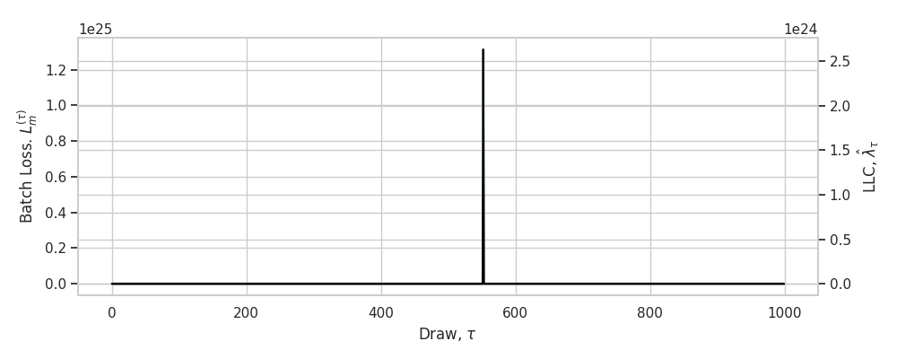
(a) Numerical instability

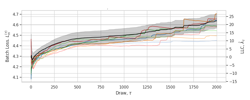
(b) Non-convergence

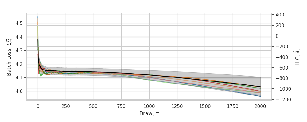
(c) Negative estimates

Figure 41: Failure modes of SGLD estimation. Top left: the gradient term is too large, leading to issues with numerical instability and exploding $\hat{\lambda}$ estimates. Top right: $\epsilon$ is too small, leading to $\hat{\lambda}$ not converging within each chain. Bottom: the localization term is too small, which allows the chain to escape to better optima.

Define $\hat{\lambda}_{\tau}(w_{0})$, the local learning coefficient at $w_{0}$ after $\tau$ time-steps for a single SGLD chain as follows Lau et al. (2023):

$$\hat{\lambda}_{\tau}(w_{0})=n\beta\left(\frac{1}{T}\sum_{t=1}^{T}L_{n}(w_{\tau})-L_{n}(w_{0})\right).$$

Moving terms around, we get,

$$\hat{\lambda}_{\tau}(w_{0}) =\frac{n}{\log n}\left(\frac{1}{\tau}\sum_{\tau^{\prime}=1}^{\tau}L_{n}(w_{\tau^{\prime}})-L_{n}(w_{0})\right)$$ (45)

$$=n\beta\left(\frac{\tau-1}{\tau}\left(\frac{1}{\tau-1}\sum_{\tau^{\prime}=1}^{\tau-1}L_{n}(w_{\tau}^{\prime})-L_{n}(w_{0})+L_{n}(w_{0})\right)+\frac{1}{\tau}L_{n}(w_{\tau})-L_{n}(w_{0})\right)$$ (46)

$$=\frac{\tau-1}{\tau}\hat{\lambda}_{\tau-1}(w_{0})+n\beta\left(\frac{1}{\tau}L_{n}(w_{\tau})+\left(\frac{\tau-1}{\tau}-1\right)L_{n}(w_{0})\right)$$ (47)

$$=\frac{1}{\tau}\left((\tau-1)\hat{\lambda}_{\tau-1}(w_{0})+n\beta\left(L_{n}(w_{\tau})-L_{n}(w_{0})\right)\right),$$ (48)

where

$$\hat{\lambda}_{0}(w_{0})=0.$$

This can be easily extended to an online estimate over chains by averaging the update $n\beta\left(L_{n}(w_{\tau})-L_{n}(w_{0})\right)$ over multiple chains.

Appendix F Additional Figures and Code

For additional figures and code, see the anonymized repository located at https://anonymous.4open.science/r/icl-0C47.

References

- Amadei et al. (1993) Amadei, A., Linssen, A. B., and Berendsen, H. J. Essential dynamics of proteins. Proteins: Structure, Function, and Bioinformatics, 17(4):412–425, 1993.
- Amari (2016) Amari, S.-i. Information Geometry and its Applications. Springer, 2016.
- Antognini & Sohl-Dickstein (2018) Antognini, J. and Sohl-Dickstein, J. PCA of high dimensional random walks with comparison to neural network training. In Advances in Neural Information Processing Systems, volume 31, 2018.
- Baldi & Hornik (1989) Baldi, P. and Hornik, K. Neural networks and principal component analysis: Learning from examples without local minima. Neural Networks, 2(1):53–58, 1989.
- Barak et al. (2022) Barak, B., Edelman, B., Goel, S., Kakade, S., Malach, E., and Zhang, C. Hidden progress in deep learning: SGD learns parities near the computational limit. In Advances in Neural Information Processing Systems, volume 35, pp. 21750–21764, 2022.
- Briggman et al. (2005) Briggman, K. L., Abarbanel, H. D., and Kristan Jr, W. Optical imaging of neuronal populations during decision-making. Science, 307(5711):896–901, 2005.
- Brown et al. (2020) Brown, T., Mann, B., Ryder, N., Subbiah, M., Kaplan, J. D., Dhariwal, P., Neelakantan, A., Shyam, P., Sastry, G., Askell, A., et al. Language models are few-shot learners. In Advances in Neural Information Processing Systems, volume 33, pp. 1877–1901, 2020.
- Bruce & Giblin (1992) Bruce, J. W. and Giblin, P. J. Curves and Singularities: A Geometrical Introduction to Singularity Theory. Cambridge University Press, 1992.
- Callen (1998) Callen, H. B. Thermodynamics and an Introduction to Thermostatistics. American Association of Physics Teachers, 1998.
- Chen et al. (2023) Chen, Z., Lau, E., Mendel, J., Wei, S., and Murfet, D. Dynamical versus Bayesian phase transitions in a toy model of superposition. Preprint arXiv:2310.06301 [cs.LG], 2023.
- Cunningham & Yu (2014) Cunningham, J. P. and Yu, B. M. Dimensionality reduction for large-scale neural recordings. Nature Neuroscience, 17(11):1500–1509, 2014.
- Eldan & Li (2023) Eldan, R. and Li, Y. TinyStories: How small can language models be and still speak coherent English? Preprint arXiv:2305.07759 [cs.CL], 2023.
- Elhage et al. (2021) Elhage, N., Nanda, N., Olsson, C., Henighan, T., Joseph, N., Mann, B., Askell, A., Bai, Y., Chen, A., Conerly, T., DasSarma, N., Drain, D., Ganguli, D., Hatfield-Dodds, Z., Hernandez, D., Jones, A., Kernion, J., Lovitt, L., Ndousse, K., Amodei, D., Brown, T., Clark, J., Kaplan, J., McCandlish, S., and Olah, C. A mathematical framework for transformer circuits. Transformer Circuits Thread, 2021.
- Erhan et al. (2010) Erhan, D., Bengio, Y., Courville, A., Manzagol, P.-A., Vincent, P., and Bengio, S. Why does unsupervised pre-training help deep learning? Journal of Machine Learning Research, 11(19):625–660, 2010.
- Franceschelli (2010) Franceschelli, S. Morphogenesis, structural stability and epigenetic landscape. In Morphogenesis: Origins of Patterns and Shapes, pp. 283–293. Springer, 2010.
- Freed (2021) Freed, D. The Atiyah–Singer index theorem. Bulletin of the American Mathematical Society, 58(4):517–566, 2021.
- Freedman et al. (2023) Freedman, S. L., Xu, B., Goyal, S., and Mani, M. A dynamical systems treatment of transcriptomic trajectories in hematopoiesis. Development, 150(11):dev201280, 2023.
- Gao et al. (2020) Gao, L., Biderman, S., Black, S., Golding, L., Hoppe, T., Foster, C., Phang, J., He, H., Thite, A., Nabeshima, N., Presser, S., and Leahy, C. The Pile: an 800GB dataset of diverse text for language modeling. Preprint arXiv:2101.00027 [cs.CL], 2020.
- Garg et al. (2022) Garg, S., Tsipras, D., Liang, P., and Valiant, G. What can transformers learn in-context? a case study of simple function classes. In Advances in Neural Information Processing Systems, 2022.
- Ghader & Monz (2017) Ghader, H. and Monz, C. What does attention in neural machine translation pay attention to? In Proceedings of the Eighth International Joint Conference on Natural Language Processing (Volume 1: Long Papers), pp. 30–39. Asian Federation of Natural Language Processing, 2017.
- Gilbert (2006) Gilbert, S. F. Developmental Biology. Sinauer Associates Inc., eighth edition, 2006.
- Gilmore (1981) Gilmore, R. Catastrophe Theory for Scientists and Engineers. Wiley, 1981.
- Goodfellow et al. (2014) Goodfellow, I. J., Vinyals, O., and Saxe, A. M. Qualitatively characterizing neural network optimization problems. Preprint arXiv:1412.6544 [cs.NE], 2014.
- Hayward & De Groot (2008) Hayward, S. and De Groot, B. L. Normal modes and essential dynamics. Molecular Modeling of Proteins, pp. 89–106, 2008.
- Jacot et al. (2021) Jacot, A., Ged, F., Şimşek, B., Hongler, C., and Gabriel, F. Saddle-to-saddle dynamics in deep linear networks: Small initialization training, symmetry, and sparsity. Preprint arXiv:2106.15933 [stat.ML], 2021.
- Jimenez Rodriguez (2018) Jimenez Rodriguez, A. The Shape of the PCA Trajectories and the Population Neural Coding of Movement Initiation in the Basal Ganglia. PhD thesis, University of Sheffield, 2018.
- Karpathy (2022) Karpathy, A. NanoGPT, 2022. URL https://github.com/karpathy/nanoGPT.
- Kingma & Ba (2014) Kingma, D. P. and Ba, J. Adam: A method for stochastic optimization. Preprint arXiv:1412.6980 [cs.LG], 2014.
- Lau et al. (2023) Lau, E., Murfet, D., and Wei, S. Quantifying degeneracy in singular models via the learning coefficient. Preprint arXiv:2308.12108 [stat.ML], 2023.
- Li et al. (2018) Li, H., Xu, Z., Taylor, G., Studer, C., and Goldstein, T. Visualizing the loss landscape of neural nets. In Advances in Neural Information Processing Systems, volume 31, 2018.
- Lipton (2016) Lipton, Z. C. Stuck in a what? adventures in weight space. Preprint arXiv:1602.07320 [cs.LG], 2016.
- MacArthur (2022) MacArthur, B. D. The geometry of cell fate. Cell Systems, 13(1):1–3, 2022.
- McGrath et al. (2022) McGrath, T., Kapishnikov, A., Tomašev, N., Pearce, A., Wattenberg, M., Hassabis, D., Kim, B., Paquet, U., and Kramnik, V. Acquisition of chess knowledge in AlphaZero. Proceedings of the National Academy of Sciences, 119(47), 2022.
- McGrath et al. (2023) McGrath, T., Rahtz, M., Kramar, J., Mikulik, V., and Legg, S. The hydra effect: Emergent self-repair in language model computations. Preprint arXiv:2307.15771 [cs.LG], 2023.
- Meyer et al. (2006) Meyer, T., Ferrer-Costa, C., Pérez, A., Rueda, M., Bidon-Chanal, A., Luque, F. J., Laughton, C. A., and Orozco, M. Essential dynamics: a tool for efficient trajectory compression and management. Journal of Chemical Theory and Computation, 2(2):251–258, 2006.
- Michaud et al. (2024) Michaud, E. J., Liu, Z., Girit, U., and Tegmark, M. The quantization model of neural scaling. Preprint arXiv:2303.13506 [cs.LG], 2024.
- Nanda & Bloom (2022) Nanda, N. and Bloom, J. TransformerLens, 2022. URL https://github.com/neelnanda-io/TransformerLens.
- Nanda et al. (2023) Nanda, N., Chan, L., Lieberum, T., Smith, J., and Steinhardt, J. Progress measures for grokking via mechanistic interpretability. In The Eleventh International Conference on Learning Representations, 2023.
- Notsawo et al. (2023) Notsawo, P. J. T., Zhou, H., Pezeshki, M., Rish, I., and Dumas, G. Predicting grokking long before it happens: A look into the loss landscape of models which grok. Preprint arXiv:2306.13253 [cs.LG], 2023.
- Olah et al. (2020) Olah, C., Cammarata, N., Schubert, L., Goh, G., Petrov, M., and Carter, S. Zoom in: An introduction to circuits. Distill, 5(3):e00024.001, March 2020.
- Olsson et al. (2022) Olsson, C., Elhage, N., Nanda, N., Joseph, N., DasSarma, N., Henighan, T., Mann, B., Askell, A., Bai, Y., Chen, A., Conerly, T., Drain, D., Ganguli, D., Hatfield-Dodds, Z., Hernandez, D., Johnston, S., Jones, A., Kernion, J., Lovitt, L., Ndousse, K., Amodei, D., Brown, T., Clark, J., Kaplan, J., McCandlish, S., and Olah, C. In-context learning and induction heads. Transformer Circuits Thread, 2022.
- Phuong & Hutter (2022) Phuong, M. and Hutter, M. Formal algorithms for transformers. Preprint arXiv:2207.09238 [cs.LG], 2022.
- Press et al. (2021) Press, O., Smith, N. A., and Lewis, M. Shortformer: Better language modeling using shorter inputs. In Proceedings of the 59th Annual Meeting of the Association for Computational Linguistics and the 11th International Joint Conference on Natural Language Processing (Volume 1: Long Papers), pp. 5493–5505. Association for Computational Linguistics, 2021.
- Raijmakers et al. (1996) Raijmakers, M. E., Van Koten, S., and Molenaar, P. C. On the validity of simulating stagewise development by means of PDP networks: Application of catastrophe analysis and an experimental test of rule-like network performance. Cognitive Science, 20(1):101–136, 1996.
- Rand et al. (2021) Rand, D. A., Raju, A., Sáez, M., Corson, F., and Siggia, E. D. Geometry of gene regulatory dynamics. Proceedings of the National Academy of Sciences, 118(38):e2109729118, 2021.
- Raventós et al. (2023) Raventós, A., Paul, M., Chen, F., and Ganguli, S. Pretraining task diversity and the emergence of non-Bayesian in-context learning for regression. Preprint arXiv:2306.15063 [cs.LG], 2023.
- Rogers & McClelland (2004) Rogers, T. T. and McClelland, J. L. Semantic Cognition: A Parallel Distributed Processing Approach. MIT Press, 2004.
- Sáez et al. (2022) Sáez, M., Blassberg, R., Camacho-Aguilar, E., Siggia, E. D., Rand, D. A., and Briscoe, J. Statistically derived geometrical landscapes capture principles of decision-making dynamics during cell fate transitions. Cell Systems, 13(1):12–28, 2022.
- Saxe et al. (2019) Saxe, A. M., McClelland, J. L., and Ganguli, S. A mathematical theory of semantic development in deep neural networks. Proceedings of the National Academy of Sciences, 116(23):11537–11546, 2019.
- Shinn (2023) Shinn, M. Phantom oscillations in principal component analysis. Proceedings of the National Academy of Sciences, 120(48):e2311420120, 2023.
- Thom (1988) Thom, R. Structural Stability and Morphogensis: An Outline of a General Theory of Models. Advanced Book Classics Series, 1988. Translated by D. H. Fowler from the 1972 original.
- Vig & Belinkov (2019) Vig, J. and Belinkov, Y. Analyzing the structure of attention in a transformer language model. Preprint arXiv:1906.04284 [cs.CL], 2019.
- Waddington (1957) Waddington, C. H. The Strategy of the Genes: A Discussion of Some Aspects of Theoretical Biology. Allen & Unwin, London, 1957.
- Wang et al. (2022) Wang, K., Variengien, A., Conmy, A., Shlegeris, B., and Steinhardt, J. Interpretability in the wild: a circuit for indirect object identification in GPT-2 small. Preprint arXiv:2211.00593 [cs.LG], 2022.
- Watanabe (2009) Watanabe, S. Algebraic Geometry and Statistical Learning Theory. Cambridge University Press, 2009.
- Wei et al. (2022) Wei, J., Tay, Y., Bommasani, R., Raffel, C., Zoph, B., Borgeaud, S., Yogatama, D., Bosma, M., Zhou, D., Metzler, D., Chi, E. H., Hashimoto, T., Vinyals, O., Liang, P., Dean, J., and Fedus, W. Emergent abilities of large language models. Transactions on Machine Learning Research, 2022.
- Xie et al. (2023) Xie, S. M., Santurkar, S., Ma, T., and Liang, P. Data selection for language models via importance resampling. Preprint arXiv:2302.03169 [cs.CL], 2023.
- Yao et al. (2020) Yao, Z., Gholami, A., Keutzer, K., and Mahoney, M. PyHessian: Neural networks through the lens of the Hessian. Preprint arXiv:1912.07145 [cs.LG], 2020.