On the Broadening of the Pulse Width of FRB 20121102A due to Propagation and Instrumental Effects

The pulse widths of fast radio bursts are always broadened due to the scattering of the plasma medium through which the electromagnetic wave passes. The recorded pulse width will be further affected by the radio telescopes since the sampling time and the bandwidth cannot be infinitely small. In this study, we focus on the pulse widths of the 3287 bursts detected from FRB 20121102A as of October 2023. Various effects such as the scattering broadening, the redshift broadening and the instrumental broadening are examined. It is found that the instrumental broadening only contributes a fraction of $10^{-3}$–$10^{-1}$ to the observed pulse width. The scattering broadening is even smaller, which constitutes a tiny fraction of $10^{-5}$–$10^{-2}$ in the observed pulse width. After correcting for these broadenings, the intrinsic pulse width is derived for each burst. The maximum and minimum pulse widths at different frequencies are highlighted. Interestingly, both the mean value and the dispersion range of intrinsic pulse width are found to be inversely proportional to the square of the central frequency. The intrinsic widths of most bursts are in a narrow range of 1–10 ms, which leads to a quasi-linear correlation between the fluence and the peak flux.

1 Introduction

Fast radio bursts (FRBs) are intensive radio transients typically lasting for a few milliseconds, with an isotropic peak luminosity up to $\sim$ $10^{38}$ to $10^{46}$ erg s^-1. Their brightness temperature is $\sim$ $10^{35}$–$10^{36}$ K, indicating that the coherent radiation mechanism should be involved (Lorimer et al. 2007; Cordes & Chatterjee 2019; Petroff et al. 2019, 2022; Zhang 2023). The dispersion measure (DM) of FRBs, which is an integration of the column density of free electrons along the line of sight, is generally much larger than the value contributed by Galactic electrons predicted by the NE2001 model, implying an extra-galactic origin for them (Cordes & Lazio 2002; Thornton et al. 2013; Yao et al. 2017). There seem to be two classes of FRBs, i.e., repeaters and non-repeating ones. Currently, more than 800 FRB sources have been detected, among which there are only ${\sim}$ 60 FRBs verified to be repeaters and ${\sim}$ 40 are well-localized (Petroff et al. 2016, 2022; CHIME/FRB Collaboration et al. 2021; Chime/Frb Collaboration et al. 2022; Hu & Huang 2023; Xu et al. 2023; Zhang 2023). However, it is still unclear whether those one-off events are really non-repeating sources or are actually also repeaters whose repeated bursts simply were not recorded by us. Among the repeaters, two sources are found to have a long-term periodicity: a possible $\sim$ 160-day periodicity exists in the activity of FRB 20121102A, and a robust 16.35-day periodicity is found for FRB 20180916B, with an activity window of ${\sim}$ 5 days (Rajwade et al. 2020; CHIME/FRB Collaboration et al. 2020; Cruces et al. 2021). Statistically, repeating FRBs generally have a relatively larger width and narrower bandwidth. They also have a complex time-frequency down-drifting behavior, generally referred to as the “sad-trombone” effect (Hessels et al. 2019; CHIME/FRB Collaboration et al. 2021; Pleunis et al. 2021).

The astrophysical origin of FRBs is still enigmatic. For repeating and one-off FRBs, many models have been proposed respectively. For example, possible models of repeating FRBs include: activities in the magnetosphere of magnetars (Beloborodov 2017, 2020; Margalit et al. 2019), giant pulses from young pulsars (Cordes & Wasserman 2016; Connor et al. 2016), and the fractional collapses of the crust of a strange star (Geng et al. 2021). On the other hand, models of non-repeating FRBs include: mergers of double neutron star systems (Dokuchaev & Eroshenko 2017) and collapses of massive neutron stars to black holes (Falcke & Rezzolla 2014; Ravi & Lasky 2014; Zhang 2018).

FRB 20121102A is the first repeating FRB source discovered by the 305 m Arecibo telescope. It has been extensively monitored by many radio telescopes. More than three thousand FRBs have been observed from this source, which provide a valuable data set for us to study the nature of FRBs. Some key parameters are available for the bursts, such as their durations, fluences, and frequency ranges. However, note that when the radio emissions of FRBs propagate toward us, they will be affected by the plasma medium along the line of sight, which will lead to various effects such as the delay of lower frequency waves and the broadening of the pulse width. The plasma medium is inhomogeneous and includes many components, i.e. the interstellar medium (ISM) of the host galaxy, the intergalactic medium (IGM), and the ISM of our Milky Way (Rickett 1990; Petroff et al. 2019). When the radio waves travel through the medium, they will be scattered, leading to the delay and broadening of the FRB pulses (Rickett 1990; Xu & Zhang 2016). In this study, we will investigate these effects for the 3287 bursts from FRB 20121102A detected by various instruments. Additionally, the radio telescopes may also lead to some broadening of the observed widths of FRBs (Cordes & McLaughlin 2003), which is usually referred to as the instrumental effect. This will also be considered in our study.

The structure of our article is organized as follows. The theory of radio wave scattering by plasma and the induced temporal broadening is introduced in Section 2, together with the introduction of the instrumental broadening. Our numerical results for the 3287 bursts from FRB 20121102A are presented and analyzed in Section 3. Finally, our conclusions and some discussion are included in Section 4.

2 Temporal Broadening

When a pulse of radio waves travel through a plasma medium, they will be affected by electron scattering, leading to some chromatic behaviors (dispersion) and the broadening of the pulse duration. As a result, the recorded pulse width by an observer can be written as (Cordes & McLaughlin 2003; Lorimer & Kramer 2012; Zhang 2023)

$$W_{\rm obs}=[{W_{\rm i}^{2}}\times(1+z_{0})^{2}+\tau_{\rm sc}^{2}+\tau_{\rm tel}^{2}]^{\frac{1}{2}},$$ (1)

where $W_{\rm i}$ is the original intrinsic pulse width, $z_{0}$ is the redshift, $\tau_{\rm sc}$ and $\tau_{\rm tel}$ are the temporal broadenings caused by plasma scattering and instrumental effects, respectively. The detailed expressions for $\tau_{\rm sc}$ and $\tau_{\rm tel}$ are presented in the subsections below.

2.1 Scattering broadening of the pulse width

The contribution of scattering broadening mainly comes from the ISM inside the host galaxy and the Milky Way. For simplicity, we assume that the medium itself is homogeneous and the intrinsic fluctuations are quasi-statistical (Barabanenkov et al. 1971). In this case, the scattering effect can be conveniently modeled by following the work of Rickett (1990).

The IGM might also contribute to the scattering and broadening effect. The turbulence spectrum index of IGM ($\beta$) is generally larger than 3 (Rickett 1990). A typical value of $\beta$ is $\frac{11}{3}$ (i.e. the Kolmogorov turbulence spectrum), and the turbulence heating rate is negligible in the Hubble time (Luan & Goldreich 2014; Xu & Zhang 2016). Consequently, in the case of FRBs, the broadening effect caused by IGM is actually extremely small, which is typically several orders of magnitude less than a millisecond. Therefore, we will neglect the IGM contribution in this study.

For a homogeneous ISM, the density fluctuation is a short-wave-dominated spectrum ($\beta<3$) and the diffractive length is smaller than the length scale of the turbulence $l_{0}$ (Xu & Zhang 2016). The scatter angle is much less than 1. Therefore, we can derive the broadening timescale induced by scattering as

$$\tau_{\rm sc}\propto\frac{\lambda_{0}^{4}DM^{2}}{(1+z_{0})^{3}}(\frac{\delta n_{\rm e}}{n_{\rm e}})^{2}l_{0}^{-1},$$ (2)

where $DM$ is the total dispersion measure along the line of sight, $\lambda_{0}$ is the wavelength of the radio emission in the observer’s frame, $\delta n_{\rm e}$ is the root-mean-square of the electron density fluctuation, and $n_{\rm e}$ is correspondingly the electron number density. Assuming that the properties of the host galaxy are similar to our Milky Way, we can replace $\delta n_{\rm e}$ with $\sqrt{f}\delta n_{\rm e}$ for the host galaxy ISM, where $f$ is the volume filling factor. Equation (2) can then be further expressed as (Xu & Zhang 2016)

$$\tau_{\rm sc}\approx\frac{0.2}{(1+z_{0})^{3}}(\frac{DM}{100\,{\rm pc\,cm^{-3}}})^{2}(\frac{\lambda_{0}}{{\rm 1m}})^{4}\\ (\frac{f}{10^{-6}})(\frac{\delta n_{\rm e}}{n_{\rm e}})^{2}(\frac{l_{0}}{10^{-10}{\rm pc}})^{-1}{\rm ms},$$ (3)

by substituting the typical values of the parameters into it.

The total dispersion measure in Equation (2) is a sum of several components (Thornton et al. 2013; Deng & Zhang 2014; Prochaska & Zheng 2019), i.e.

$$DM=DM_{\rm MW}+DM_{\rm halo}+DM_{\rm IGM}+\frac{DM_{\rm host}}{1+z_{0}},$$ (4)

where $DM_{\rm MW}$, $DM_{\rm halo}$, $DM_{\rm IGM}$ and $DM_{\rm host}$ are the contributions from the Milky Way, the Galactic halo, the IGM and the host, respectively. For our Galaxy, we have $DM_{\rm MW}=188\,{\rm pc\,cm^{-3}}$ and $DM_{\rm halo}=30\,{\rm pc\,cm^{-3}}$. IGM contribution at $z_{0}<3$ can be calculated by using a linear formula (Zhang 2018; Pol et al. 2019; Cordes et al. 2022)

$$<DM_{\rm IGM}>=(855\,{\rm pc\,cm^{-3}})z_{0}\frac{H_{0}}{67.74\,{\rm km\,s^{-1}\,kpc^{-1}}}\\ \frac{\Omega_{\rm b}}{0.0486}\frac{f_{\rm IGM}}{0.83}\frac{\chi}{7/8},$$ (5)

where $H_{0}$ is the Hubble constant, $\Omega_{b}$ is the energy density fraction of baryons, $f_{\rm IGM}$ is the mass fraction of baryons in the IGM, and $\chi$ is the fraction of ionized electrons.

2.2 Instrumental broadening

The radio telescope can also have a complex effect on the observed pulse width. It depends on the DM of the source, the bandwidth of each frequency channel, and the sampling time. To be more specific, the instrumental broadening term of $\tau_{\rm tel}$ in Equation (1) can be written as (Cordes & McLaughlin 2003; Petroff et al. 2019)

$$\tau_{\rm tel}=[\Delta\tau_{\rm DM}^{2}+\Delta\tau_{\rm\delta DM}^{2}+\Delta\tau_{\Delta\nu}^{2}+\tau_{\rm samp}^{2}]^{\frac{1}{2}}.$$ (6)

Here, the first term, $\Delta\tau_{\rm DM}$, is the frequency-dependent intra-channel dispersive smearing, which is further expressed as (Cordes & McLaughlin 2003)

$$\Delta\tau_{\rm DM}=8.3DM\Delta\nu_{\rm MHz}\nu_{\rm GHz}^{-3}\,\,\mu{\rm s},$$ (7)

where $\Delta\nu_{\rm MHz}$ is the bandwidth of the channel (in units of MHz) and $\nu_{\rm GHz}$ is its central frequency (in units of GHz).

The second term in Equation (6) originates from the deviations (i.e. $\delta DM$) between the true DM and the fiducial DM, which is chosen to de-disperse the channels coherently (Hessels et al. 2019). It can be expressed as (Cordes & McLaughlin 2003)

$$\Delta\tau_{\rm\delta DM}={\Delta\tau_{\rm DM}}\frac{\delta DM}{DM}.$$ (8)

The third term in Equation (6) is the so-called bandwidth smearing (Bridle & Schwab 1999; Rioja et al. 2018), which can be approximately calculated as

$$\Delta\tau_{\Delta\nu}\sim(\Delta\nu_{\rm MHz})^{-1}\,\,\mu{\rm s}.$$ (9)

Finally, the fourth term of $\tau_{\rm samp}$ in Equation (6) is simply the sampling time.

3 Numerical Results for FRB 20121102A

As the first repeating FRB source discovered by Arecibo, FRB 20121102A has been extensively monitored by many radio telescopes. The source is associated with a low-metallicity dwarf galaxy at a redshift of ${\sim}$ 0.193, located in the vicinity of a star-forming region (Cordes et al. 2006; Spitler et al. 2014, 2016; Lazarus et al. 2015; Chatterjee et al. 2017; Tendulkar et al. 2017; Marcote et al. 2017). The DM of FRB 20121102A was measured as 557.4 ${\pm}$ 2.0 pc cm^-3 on MJD 56233, and has increased to 565.8 ${\pm}$ 0.9 pc cm^-3 between MJD 58724 and MJD 58776, showing an increasing trend of ${\sim}$ 1 pc cm^-3 year^-1 (Spitler et al. 2014, 2016; Li et al. 2021). A linear polarization of nearly 100 percent was detected, with the polarization angle being almost constant (Michilli et al. 2018; Plavin et al. 2022; Hewitt et al. 2022). In the meantime, the rotation measure (RM) of FRB 20121102A has changed drastically from 1.46 ${\times}$ 10⁵ rad m^-2 to 7 ${\times}$ 10⁴ rad m^-2 over three years, which could point to the existence of an extreme magneto-ionic environment related to an accreting compact star, or a magnetized wind nebula around a magnetar (Spitler et al. 2016; Michilli et al. 2018). In addition, other environment models have been proposed, such as the binary interactions involving a neutron star Wang et al. 2022. As of October 2023, a total number of 3287 bursts have been detected from FRB 20121102A by various telescopes. We have collected the main observational parameters of all these events. An overview of our data set is presented in Table 1.

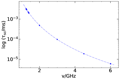
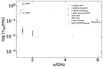
Figure 1: The scattering broadening (left panel) and instrumental broadening (right panel) plotted versus the observing frequency.

For the 3287 bursts of FRB 20121102A, we have analyzed the broadening of their pulse widths caused by different factors. Figure 1 shows the scattering broadening and instrumental broadening at different observing frequencies. In the left panel, we see that the scattering broadening is generally a power-law function of the frequency, i.e. $\tau_{\rm sc}\propto\nu^{-4}$, which is consistent with Equation (3). It can also be seen that the broadening ranges between $10^{-5}$ ms–$3\times 10^{-3}$ ms, which means this effect is essentially very small. The instrumental broadening versus the observing frequency is plotted in the right panel of Figure 1. We see that $\tau_{\rm tel}$ is generally between $10^{-2}$ ms to 1 ms, which is about three magnitudes larger than the scattering broadening. It could be expected that this effect will be significant for short FRBs, especially those lasting for less than 1 ms.

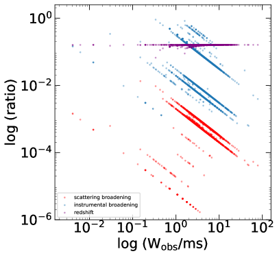
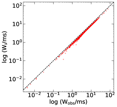
Figure 2: Various broadening effects on the bursts of FRB 20121102A. The first panel shows the ratio of pulse width broadening due to the redshift, scattering and instrumental effects (marked by different colors). The second panel plots the intrinsic pulse width versus the observed width. The dashed line corresponds to $W_{\rm obs}=W_{\rm i}$.

In the first panel of Figure 2, the fractions of pulse width broadening due to the redshift, scattering and instrumental effects are illustrated by different colors. Since FRB 20121102A is at a redshift of $z\sim 0.193$, we see that the redshift-induced broadening ratio is typically $\sim 0.16$ (the purple dots). The ratio of instrumental broadening generally ranges between $10^{-3}$–0.1. However, for some bursts, the ratio can be larger than 60%. They are mainly short events whose duration is less than 1 ms. In these cases, the sampling time could seriously affect the measured pulse width. Furthermore, we see that the ratio of scattering broadening generally ranges between $10^{-5}$–$10^{-2}$. It is much smaller than the instrumental broadening as a whole. After solving the effects of these factors, we can then easily correct them and derive the intrinsic pulse width, i.e. $W_{\rm i}$. The second panel of Figure 2 plots $W_{\rm i}$ versus the observed width. Here, the dashed line corresponds to $W_{\rm i}=W_{\rm obs}$. We see that most of the data points are very close to the dashed line, which means that the effects of all three broadening factors (i.e. redshift, scattering and instrumental effects) are unimportant for the majority of FRBs. The broadening is noticeable only for a very small portion of FRBs. They are typically short events that are more seriously subjected to the influence of the sampling time.

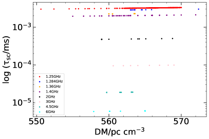
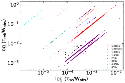
Figure 3: The absolute values of scattering broadening and its ratio compared with that of the instrumental broadening. The first panel plots the scattering broadening versus $DM$. The second panel shows the ratio of the scattering broadening (with respect to the total observed width, i.e. $\tau_{\rm{sc}}/W_{\rm obs}$) versus the ratio of the instrumental broadening (i.e. $\tau_{\rm{tel}}/W_{\rm obs}$).

Figure 3 shows the absolute values of scattering broadening ($\tau_{\rm sc}$) and its ratio compared with that of the instrumental broadening. In the first panel, we see that there is a linear relation between $\tau_{\rm sc}$ and $DM$, which can be inferred from Equation (3). However, since $DM$ itself does not vary too much in this source, $\tau_{\rm sc}$ also only varies slightly at any particular frequency. As a result, $\tau_{\rm sc}$ is mainly determined by the observing frequency. Anyway, $\tau_{\rm sc}$ is generally in the range of $10^{-5}$–$10^{-3}$ ms. It plays a minor role in the broadening. In the second panel of Figure 3, we see that when the ratio of scattering broadening is plotted versus the ratio of instrumental broadening, all bursts detected by the same instrument distribute on a straight line with a slope of about 1. The intercept of the line depends on many parameters such as $DM$, $\lambda_{0}$, $\Delta\nu_{\rm MHz}$ and $\tau_{\rm samp}$.

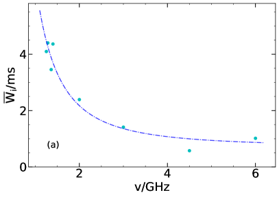
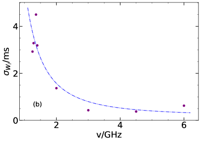
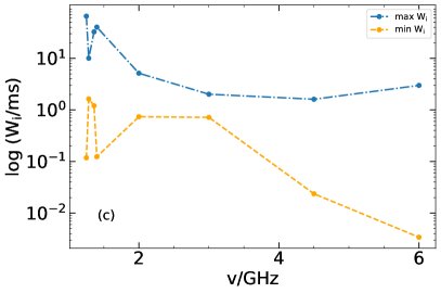
Figure 4: Characteristics of the intrinsic pulse widths based on subsample analysis. Here the FRBs are divided into subsamples according to the telescopes that detected them. Panel (a): the mean intrinsic pulse width of each subsample ($\overline{W}_{\rm i}$) plotted versus the central frequency; Panel (b): the dispersion range of the intrinsic pulse width ($\sigma_{\rm W_{i}}$) plotted versus frequency for each subsample; Panel (c): the maximum and minimum values of the intrinsic pulse width in each subsample versus frequency.

Figures 1–3 clearly show that while the broadening of FRBs is determined by the source parameters such as $DM$, it is more significantly dependent on the conditions of the instruments ($\lambda_{0}$, $\Delta\nu_{\rm MHz}$ and $\tau_{\rm samp}$). Therefore, we need to divide the 3287 bursts into subsamples according to the radio telescopes that detected them and analyze these subsamples separately. Our results based on subsample analysis of the intrinsic pulse width are illustrated in Figure 4. Figure 4a plots the mean intrinsic pulse width ($\overline{W}_{\rm i}$) versus the central frequency of the FRBs. We see that $\overline{W}_{\rm i}$ obviously has a decreasing tendency when the frequency increases. It declines from $\sim 4.5$ ms at 1.3 GHz to $\sim 1$ ms at 6 GHz and generally follows a function of $\overline{W}_{\rm i}\propto\nu^{-2}$. In fact, the best-fit curve of the data points corresponds to

$$\frac{\overline{W}_{\rm i}}{1{\rm ms}}=5.9\left(\frac{\nu}{1{\rm Ghz}}\right)^{-2}+0.7.$$ (10)

Figure 4b plots the dispersion range of the intrinsic pulse width ($\sigma_{\rm W_{i}}$) versus the central frequency. Interestingly, $\sigma_{\rm W_{i}}$ also has a decreasing tendency when the frequency increases. It also declines from $\sim 4.5$ ms at 1.3 GHz to $\sim 1$ ms at 6 GHz, and also scale as $\sigma_{\rm W_{i}}\propto\nu^{-2}$. The best-fit curve of the data points corresponds to

$$\frac{\sigma_{\rm W_{i}}}{1{\rm ms}}=5.6\left(\frac{\nu}{1{\rm Ghz}}\right)^{-2}+0.2.$$ (11)

Figure 4c shows the maximum and minimum values of the intrinsic pulse width in each subsample. At a frequency of $\nu<2$ GHz, the minimum width is about 0.1 ms, while the maximum width can be up to $\sim 65$ ms. At 6 GHz, the minimum width is as short as $\sim 3\times 10^{-3}$ ms and the maximum width is $\sim 3$ ms. The maximum and minimum widths can put stringent constraints on the trigger mechanism and radiation process of FRBs. A successful FRB model should be capable of explaining these extreme values.

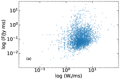
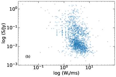
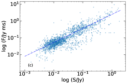
Figure 5: Overall features of the FRBs. Panel (a): FRBs on the $F$-$W_{\rm i}$ plane; Panel (b): FRBs on the $S$-$W_{\rm i}$ plane; Panel (c): FRBs on the $F$-$S$ plane.

The peak flux ($S$), fluence ($F$) and pulse width are three key parameters of FRBs. After acquiring the intrinsic pulse width, we can explore any possible connection between the parameters. Figure 5 shows the distribution of FRBs when one parameter is plotted versus another. From Figure 5a, we see that the distribution of the FRBs on the $F$-$W_{\rm i}$ plane is quite chaotic so that no correlation exists between these two parameters. Another feature is that the pulse widths of the majority of FRBs are distributed in a relatively narrow range ($\sim 1$–10 ms). On the contrary, the distribution range of fluence is much wider, which spans over two magnitudes ($\sim 0.01$–1 Jy ms). Figure 5b shows that there seems to exist a weak negative correlation between the peak flux and the intrinsic pulse width: a longer FRB tends to have a smaller peak flux. However, the correlation is generally too weak to draw any firm conclusion. Similarly, we notice that the peak flux also has a relatively large distribution range, which spans over two magnitudes (mainly in a range of $\sim 3\times 10^{-3}$–$3\times 10^{-1}$ Jy). Figure 5c plots the fluence ($F$) versus the peak flux ($S$). We see that there is an obvious positive correlation between these two parameters. A bet fit of the data points gives

$$\frac{F}{1{\rm Jy\,ms}}=3\left(\frac{S}{1{\rm Jy}}\right)^{0.8}.$$ (12)

In fact, $F$ can be regarded as a product of the peak flux and the equivalent pulse width. The above positive correlation is a natural outcome giving the fact that the intrinsic pulse widths of FRBs are narrowly distributed in a small range.

We have also divided the FRBs into several groups according to their central frequency (i.e. 1.25 GHz, 1.36 GHz, 1.4 GHz, 4.5 GHz and 6 GHz groups). The distribution of the observed/intrinsic pulse width is compared for each group to present a direct illustration of the broadening effects. Figure 6 plots the histogram distributions of the observed pulse width and the corrected intrinsic pulse width for each group. A Gaussian fit is performed for each distribution, which gives the most probable width ($\mu_{\rm i},\mu_{\rm obs}$) and the dispersion range ($\sigma_{\rm i},\sigma_{\rm obs}$) of the bursts at these frequencies. The derived parameters are listed in Table 2. The intrinsic pulse widths are slightly smaller than the observed width, but their distributions do not differ from each other significantly.

4 Conclusions and Discussion

With more and more FRB sources being detected, it is necessary to systematically analyze the statistical features of their intrinsic parameters. In this study, we have collected all the 3287 bursts detected from FRB 20121102A as of October 2023. Various broadening effects on the pulse width, including the scattering broadening caused by turbulence and the instrumental broadening induced during observations, are considered and corrected. It is found that these broadening effects do not play a dominant role in the majority of bursts from FRB 20121102A. The instrumental broadening is mainly in a range of $10^{-2}$–1 ms, which contributes a fraction of $10^{-3}$–$10^{-1}$ to the observed pulse width. The scattering broadening is even smaller, which mainly ranges in $10^{-5}$–$10^{-3}$ ms and only contributes a fraction of $10^{-5}$–$10^{-2}$ to the observed pulse width. Interestingly, the mean intrinsic pulse width is found to decrease as the central frequency increases, i.e. $\overline{W}_{\rm i}\propto\nu^{-2}$. More strikingly, the dispersion range of the intrinsic pulse width also has a similar behavior, $\sigma_{\rm W_{i}}\propto\nu^{-2}$. Such a frequency-dependent behavior of $\overline{W}_{\rm i}$ and $\sigma_{\rm W_{i}}$ may place useful constraints on the triggering mechanism and radiation process of FRBs. A quasi-linear correlation exists between the fluence and the peak flux, which is mainly due to the narrow distribution of the intrinsic pulse width for the majority of the bursts.

Although the scattering broadening seems to be insignificant in the case of FRB 20121102A, it may still play an important role in other FRB sources. In fact, from Equation (2), we see that the scattering broadening scales as $\tau_{\rm sc}\propto\lambda_{0}^{4}DM^{2}(\frac{\delta n_{\rm e}}{n_{\rm e}})^{2}l_{0}^{-1}$. So, it sensitively depends on many parameters, such as the observing frequency, the total dispersion measure, the turbulence scale, and the density fluctuations. Especially, when the central frequency decreases to 300 MHz, the scattering broadening will be enlarged by a factor or $\sim 120$. Note that the instrumental broadening may also be significantly amplified at low frequencies (see Equation (7)). As a result, these broadening effects should still be paid attention to in other FRB sources as long as the pulse width is involved.

Turbulence is also a complex factor that could seriously affect the two ISM parameters in Equation (2), i.e. $l_{0}$ and $\delta n_{\rm e}$. Additionally, note that the spectrum index of turbulence ($\beta$) may also have some effects on the scattering broadening. In practice, when an FRB is detected by a radio telescope, the dynamical spectrum (or the so-called “waterfall” diagram) is usually available, which may contain rich information on the turbulence of the ISM. A detailed analysis of the dynamical spectrum may help determine these parameters. On the other hand, we have mainly considered the situation where the diffractive length of the ISM is smaller than $l_{0}$. In realistic cases, the diffractive length could also be larger than $l_{0}$. It may lead to some differences in the scattering broadening, which need to be addressed in the future.

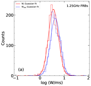
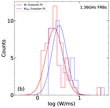
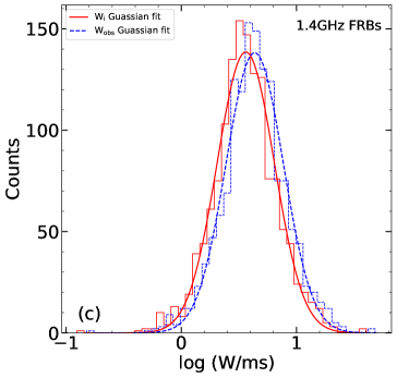
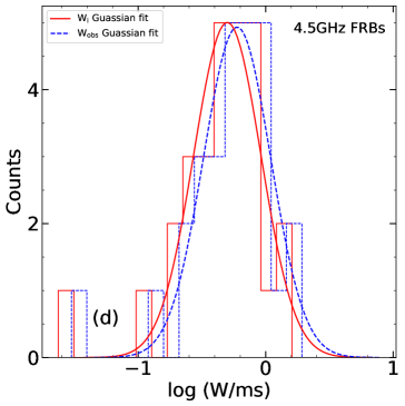
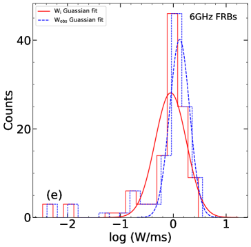
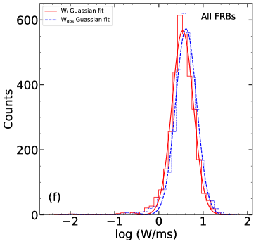
Figure 6: The distribution of the observed/intrinsic pulse width for the five groups centered at 1.25 GHz (Panel a), 1.36 GHz (Panel b), 1.4 GHz (Panel c), 4.5 GHz (Panel d) and 6 GHz (Panel e). The corresponding distribution of all the bursts as a whole is also plotted in Panel (f). The dashed curves correspond to the observed pulse width distribution and the solid curves correspond to the intrinsic width distribution. A log-norm fit is performed on each histogram and is illustrated by the corresponding solid or dashed curve.

Table 1: An overview of the observations and the corresponding telescope parameters

Telescope	Central Frequency/GHz	$\Delta\nu_{\rm MHz}$	$\tau_{\rm samp}$/ms	Burst Counts	Ref.
FAST	1.25	0.122	0.098304	1652	(1)
Arecibo	1.4	0.34/1.56	0.655/0.01024	11/1360	(2),(3),(4),(5),(6),(7),(8)
	4.5	1.56	0.01024	29	(9),(10)
GBT	2	1.56	0.01024	19	(11)
	6	0.183/0.366/2.9296875	0.01024/0.35/0.0003413	2/93/19	(9),(12),(13)
Effelsberg	1.36	0.5859375	0.054613	49	(14),(15)
	6	0.976562	0.131	1	(10)
VLA	3	0.25/4	1.024/5	2/9	(10),(16)
WSRT	1.4	0.78125/0.1953125	0.00128/0.08192	29/1	(17)
MeerKAT	1.284	0.208984375	0.004785	11	(18)

• Ref. (1) Li et al. 2021; (2) Spitler et al. 2016; (3) Hewitt et al. 2022; (4) Jahns et al. 2023; (5) Hessels et al. 2019; (6) Scholz et al. 2017; (7) Gourdji et al. 2019; (8) MAGIC Collaboration et al. 2018; (9) Michilli et al. 2018; (10) Hilmarsson et al. 2021; (11) Scholz et al. 2016; (12) Zhang et al. 2018; (13) Snelders et al. 2023; (14) Cruces et al. 2021; (15) Hardy et al. 2017; (16) Law et al. 2017; (17) Oostrum et al. 2020; (18) Caleb et al. 2020.

Table 2: The best-fit parameters for the log-normal distribution of bursts in each frequency group

Central Frequency/GHz	$\mu_{\rm i}$/ms	$\sigma_{\rm i}$/ms	$\mu_{\rm obs}$/ms	$\sigma_{\rm obs}$/ms
All	3.47	1.74	4.07	1.74
1.25	3.55	1.58	4.27	1.58
1.36	2.51	1.58	3.24	1.51
1.4	3.63	1.78	4.37	1.78
4.5	0.50	1.82	0.60	1.82
6	0.89	2.00	1.32	1.55