Intrinsic bispectrum of the scalar-induced gravitational waves

Abstract

Recent pulsar timing array collaborations have reported evidence of the stochastic gravitational wave background. The gravitational waves induced by primordial curvature perturbations, referred to as scalar-induced gravitational waves (SIGWs), could potentially be the physical origins of this gravitational wave background. In addition to the statistical properties of SIGWs derived from the primordial fluctuations, SIGWs also have intrinsic non-Gaussianity originating from the non-linear interactions of Einstein’s gravity, which, however, is rarely explored. In this paper, we study the intrinsic non-Gaussianity of SIGWs with the bispectrum and the skewness under the assumption of the Gaussian primordial curvature perturbations, phenomenologically modeled as a lognormal spectrum. The bispectrum is shown to be vanishing in the collinear limit, which is independent of the initial conditions and the dynamics of SIGWs. For the SIGWs generated during the radiation-dominated era, the bispectrum is of flatten-type non-Gaussianity, with only four polarization components left to be non-vanishing. Additionally, in order to obtain the correct bispectrum, we also propose a time-oscillation average scheme and a regularization scheme. Utilizing the skewness for quantifying the degree of non-Gaussianity, it is found that the curvature power spectrum with a narrow width can result in an enhancement of the third-order non-Gaussianity. The conclusion holds for both the SIGWs generated in the radiation-dominated era and the matter-dominated era.

I Introduction

Recent pulsar timing array (PTA) collaborations have reported evidence of the stochastic gravitational wave background (SGWB) by observing the Hellings-Downs curves Hellings and Downs (1983); Agazie et al. (2023a); Antoniadis et al. (2023a); Reardon et al. (2023); Xu et al. (2023). Revealing the origins of the observed SGWB can be considerably interesting because it is promising as a probe for studying cosmology at the early time Afzal et al. (2023); Antoniadis et al. (2023b) or phenomena in astrophysics Agazie et al. (2023b, c); Antoniadis et al. (2023c). Notably, recent statistical analyses from PTA collaborations have suggested that the cosmological origin of SGWB, such as the scalar-induced gravitational waves (SIGWs) Ananda et al. (2007); Baumann et al. (2007); Espinosa et al. (2018); Kohri and Terada (2018), seem to be more favored than the standard interpretation in astrophysics, i.e., the superposition of the gravitational waves produced by inspiring supermassive black hole binaries Antoniadis et al. (2023b); Afzal et al. (2023). Although further evidence would be required, it was expected by pioneers recently that we may be at the beginning of the era of observational gravitational wave cosmology Harigaya et al. (2023).

Because of the stochastic nature of SGWB, the statistical properties can provide lots of information on GW sources. The central limit theorem indicates that SGWB from astrophysical origin should be Gaussian because the individual source, such as supermassive black hole binaries, is reckoned as an independent system. On the cosmological side, the inflation theory suggests that the cosmological perturbations originate from quantum fluctuations Guth and Pi (1982); Starobinsky (1982), and the statistical properties of SGWBs here are derived from the primordial fluctuations Grishchuk (1974); Starobinsky (1979); Thomas et al. (2023); Cai (2023); Peng et al. (2022); Cai and Piao (2022); Fumagalli et al. (2022); Cai and Piao (2021); Ito et al. (2021). Therefore, it is motivated to explore the non-Gaussianity of the inflationary GWs Maldacena (2003); Bartolo et al. (2004, 2021); Aoki et al. (2021); Adshead and Lim (2010), as well as SIGWs generated by non-Gaussian primordial curvature perturbations Cai et al. (2019); Inomata et al. (2021); Atal and Domènech (2021); Yuan and Huang (2021); Adshead et al. (2021); Ragavendra (2022); Rezazadeh et al. (2022); Zhang (2022); Lin et al. (2023); Meng et al. (2022); Chen et al. (2022); Abe et al. (2023); Chang et al. (2023). Recently, the effect of the non-Gaussian curvature perturbations was extended to the studies on the anisotropies of SIGWs Bartolo et al. (2019, 2020); Li et al. (2023a, b). In addition to the non-Gaussianity related to the primordial universe, SIGW itself is a non-Gaussian stochastic variable due to the self-interaction of gravity. Namely, there is intrinsic non-Gaussianity of SIGWs even when the sourced primordial curvature perturbation is set to be a Gaussian variable. Similar mechanism has been found in the studies on large-scale structure Verde et al. (2000). However, the intrinsic non-Gaussianity of SIGWs is rarely explored to date

Recent interest in SIGWs stems from the potential existence of a large primordial curvature perturbation on a small scale Ananda et al. (2007); Baumann et al. (2007); Espinosa et al. (2018); Kohri and Terada (2018); Sasaki et al. (2018); Domènech (2021). In this situation, the amplitude of SIGWs can be significantly enhanced, thereby improving the detectability of GW strains. Moreover, the peaked or enhanced curvature perturbation can also result in an enhancement of the anisotropies of SIGWs Bartolo et al. (2020); Li et al. (2023a, b), and might lead to primordial black hole overproduction Afzal et al. (2023); Franciolini et al. (2023); Dandoy et al. (2023); Gorji et al. (2023); Balaji et al. (2023); Harigaya et al. (2023). Hence, this motivates us to examine whether the large curvature perturbations can also enhance the intrinsic non-Gaussianity of SIGWs.

On the observational side, the feasibility of detecting non-Gaussian SGWB was explored in the GW detectors, such as LISA satellites Bartolo et al. (2018), and PTAs Tsuneto et al. (2019); Powell and Tasinato (2020); Tasinato (2022); Zhu (2023). The presence of non-Gaussianity in SGWB might lead to a non-vanishing bispectrum for the detector’s output Bartolo et al. (2018); Tsuneto et al. (2019); Powell and Tasinato (2020) and can influence the Hellings-Downs curves Tasinato (2022); Zhu (2023). The detectability serves as the second motivation of our study on the non-Gaussianity of SIGWs.

In this study, we investigate the intrinsic non-Gaussianity of SIGWs within a phenomenological framework. We employ the log-normal power spectrum for the curvature perturbations and subsequently compute the bispectrum and skewness. For SIGWs generated during the matter-dominated era, it shows that the bispectrum amplitude decreases with the width of the curvature power spectrum. In the case of SIGWs generated during the radiation-dominated era, we must introduce an oscillation average scheme and a regularization scheme for calculating the bispectrum. It indicates that the time oscillation of GWs not only suppresses the bispectrum amplitude but also leads to a flattened-type shape of the bispectrum ($k_{3}\approx k_{1}+k_{2}$). It supports the assumption of a small intrinsic non-Gaussianity, as suggested in Ref. Bartolo et al. (2020). Additionally, the bispectrum in the colinear limit vanishes for both the matter-dominated era and the radiation-dominated era. The polarization components of the bispectrum are not independent. Specifically, the $\times\times\times$, $++\times$, $+\times+$, and $\times++$ components of the bispectrum are shown to be vanishing for the radiation-dominated era, and much smaller than the other components by three orders of magnitude for the matter-dominated era. Finally, we calculate skewness for quantifying the degree of the third-order non-Gaussianity in SIGWs, it is found that the curvature power spectrum with a narrow width can enhance the intrinsic non-Gaussianity of SIGWs.

The rest of the paper is organized as follows. In Sec. II, we enumerate relevant formulas about the dynamics of SIGWs from previous studies. These formulas will be utilized for computing the bispectrum. In Sec. III, we present the computation of the bispectra, including the cases of the colinear limit and the triangle configuration. And, for the triangular bispectrum, results for the matter-dominated era and radiation-dominated era are also presented. In Sec. IV, we calculate the skewness using the derived bispectrum and study its relation with the width of the curvature power spectrum. In Sec. V, the conclusions and discussions are summarized.

II scalar-induced gravitational waves

Since we have little knowledge about the universe at the moment after the exit of the inflationary era, there are possibilities of the existence of enhanced curvature perturbations on small scale. It can consequently lead to a large energy density of SIGWs Sasaki et al. (2018); Domènech (2021). In this section, we will enumerate the essential formulas that will be used in the computation of the bispectrum. Most of them can be found in pioneers’ studies Ananda et al. (2007); Baumann et al. (2007); Espinosa et al. (2018); Kohri and Terada (2018).

II.1 Evolution of scalar-induced gravitational waves

To evaluate the Einstein field equation in cosmological perturbation theory, the metric is expanded perturbatively in the conformal Newtonian gauge, ${\rm d}s^{2}=a^{2}(\eta)\Big{(}-(1+2\phi){\rm d}t^{2}+\big{(}\delta_{ij}(1+2\psi)+\frac{1}{2}h_{ij}\big{)}{\rm d}x^{i}{\rm d}x^{j}\Big{)}$, where $a$ is the conformal scalar factor, $h_{ij}$ is the secondary gravitational wave, $\psi$ and $\phi$ are the curvature and Newton potential perturbations, respectively. They are also referred to as the scalar perturbations. After the exit of the inflationary era, the matter filed in the universe could be effectively considered as perfect fluids. Thus, one can obtain the Einstein field equations in the second order for SIGWs as $h_{ij}^{\prime\prime}+2\mathcal{H}h_{ij}^{\prime}-\Delta h_{ij}=-4\Lambda^{ab}_{ij}\mathcal{S}_{ab},$ where $\mathcal{H}$ is the conformal Hubble parameter, and the effective source term is

$$\mathcal{S}_{ab} = \frac{2(5+3w)}{3(1+w)}\partial_{a}\psi\partial_{b}\psi+\frac{4}{3(1+w)\mathcal{H}}(\partial_{a}\psi\partial_{b}\psi^{\prime}+\partial_{a}\psi^{\prime}\partial_{b}\psi^{\prime})+\frac{4}{3(1+w)\mathcal{H}^{2}}\partial_{a}\psi^{\prime}\partial_{b}\psi^{\prime}\leavevmode\nobreak\ .$$ (1)

Given a constant equation of state parameter $w$, the conformal Hubble parameter can be evaluated to be $\mathcal{H}=2((1+3w)\eta)^{-1}$. The evolution equation of the curvature perturbations is $\psi^{\prime\prime}+3(1+c_{s}^{2})\mathcal{H}\psi^{\prime}+3(c_{s}^{2}-w)\mathcal{H}^{2}\psi-c_{s}^{2}\Delta\psi=0$, where $c_{s}$ is the speed of sound.

In Fourier space, as the equation for $h_{ij}$ reduces to an ordinary differential equation with respect to conformal time $\eta$, the solution for Fourier modes of $h_{ij}$ can take the form of

$$h_{ij,\textbf{k}} = \int\frac{{\rm d}^{3}p}{(2\pi)^{3}}\left\{\Psi_{\textbf{k}-\textbf{p}}\Psi_{\textbf{p}}\Theta_{ij}\left(\textbf{k},\textbf{p}\right)I_{h}\left(\left|\textbf{k}-\textbf{p}\right|,\left|\textbf{p}\right|,k,\eta\right)\right\}\leavevmode\nobreak\ ,$$ (2)

where $\Theta_{ij}(\mathbf{k},\mathbf{p})\equiv k^{-2}\Lambda^{ab}_{ij}(\hat{k})p_{a}p_{b}$, $\Lambda^{ab}_{ij}(\hat{k})$ is the transverse-traceless operator, $\Psi_{\mathbf{k}}$ is the initial curvature perturbations. One might find that $\Theta_{ij}(\mathbf{k},\mathbf{p})=\Theta_{ij}(\pm\mathbf{k},\pm\mathbf{p})$ and $\Theta_{ij}(\mathbf{k},\mathbf{p})=\Theta_{ij}(\mathbf{k},\mathbf{p}+\alpha\mathbf{k})$ for an arbitrary number $\alpha$. In physics, $\Psi$ is related to primordial curvature perturbations $\zeta$ through $\Psi=({3(1+w)}/{(5+3w)})\zeta$. The kernel function $I_{h}(|\mathbf{k}-\mathbf{p}|,p,k,\eta)$ can be given by

$$I_{h}\left(\left|\textbf{k}-\textbf{p}\right|,p,k,\eta\right) = \int_{0}^{\eta}{\rm d}\bar{\eta}\Bigg{\{}4k^{2}G_{k}(\eta,\bar{\eta})$$ (3)

$$\times\left(\frac{2(5+3w)T_{\textbf{k}-\textbf{p}}T_{\textbf{p}}}{3(1+w)}+\frac{4\left(T_{\textbf{k}-\textbf{p}}T^{\prime}_{\textbf{p}}+T^{\prime}_{\textbf{k - p}}T_{\textbf{p}}\right)}{3(1+w)\mathcal{H}}+\frac{4T^{\prime}_{\textbf{k}-\textbf{p}}T^{\prime}_{\textbf{p}}}{3(1+w)\mathcal{H}^{2}}\right)\Bigg{\}}\leavevmode\nobreak\ ,$$

where $T_{\textbf{k}}(\eta)$ is the transfer function of the curvature perturebations, namely, $\psi_{\textbf{k}}\equiv\Psi_{\textbf{k}}T_{\textbf{k}}(\eta)$. In this sense, one can find $I_{h}\left(\left|\textbf{k}-\textbf{p}\right|,p,k,\eta\right)=I_{h}\left(p,\left|\textbf{k}-\textbf{p}\right|,k,\eta\right)$.

In the radiation-dominated era, as the conformal time $\eta$ approaches infinity, the secondary gravitational wave exhibits behavior akin to relativistic radiation. In this case, the kernel function reduces to

$$I_{h}\left(\left|\textbf{k}-\textbf{p}\right|,p,k,\eta\right) \simeq \frac{1}{k\eta}\left(\cos(k\eta)I_{A}\left(\left|\textbf{k}-\textbf{p}\right|,\left|\textbf{p}\right|,k\right)+\sin(k\eta)I_{B}\left(\left|\textbf{k}-\textbf{p}\right|,\left|\textbf{p}\right|,k\right)\right)$$ (4)

$$\equiv I^{({\rm RD})}_{h}\left(\left|\textbf{k}-\textbf{p}\right|,\left|\textbf{p}\right|,k,\eta\right)\leavevmode\nobreak\ ,$$

where

$$I_{A}\left(\left|\textbf{k}-\textbf{p}\right|,p,k\right) \equiv \frac{27\pi\left(3k^{2}-\left|\textbf{k}-\textbf{p}\right|^{2}-p^{2}\right)^{2}}{8\left|\textbf{k}-\textbf{p}\right|^{3}p^{3}}\left({\rm sign}\left(3k-\sqrt{3}\left|\textbf{k}-\textbf{p}\right|-\sqrt{3}p\right)-1\right)\leavevmode\nobreak\ ,$$ (5a)

$$I_{B}\left(\left|\textbf{k}-\textbf{p}\right|,p,k\right) \equiv \frac{27\left(3k^{2}-\left|\textbf{k}-\textbf{p}\right|^{2}-p^{2}\right)}{4\left|\textbf{k}-\textbf{p}\right|^{3}p^{3}}\Bigg{(}4\left|\textbf{k}-\textbf{p}\right|p$$ (5b)

$$+\left(3k^{2}-\left|\textbf{k}-\textbf{p}\right|^{2}-p^{2}\right)\ln\left|\frac{3k^{2}+\left(\left|\textbf{k}-\textbf{p}\right|+p\right)^{2}}{3k^{2}+\left(\left|\textbf{k}-\textbf{p}\right|-p\right)^{2}}\right|\Bigg{)}\leavevmode\nobreak\ .$$

Similarly, in the matter-dominated era, we have

$$I_{h}\left(\left|\textbf{k}-\textbf{p}\right|,p,k,\eta\right) = \frac{40((k\eta)^{3}+2k\eta\cos(k\eta)-3\sin(k\eta))}{3(k\eta)^{3}}\equiv I^{({\rm MD})}_{h}(k,\eta)\leavevmode\nobreak\ .$$ (6)

In contrast to the situation for the radiation-dominated era, the $I_{h}^{({\rm MD})}(k,\eta)$ tends to be a constant at the late time.

II.2 Statistics of the scalar-induced gravitational waves

The power spectrum $P_{h}^{\lambda_{1}\lambda_{2}}$ for the gravitational waves $h_{ij,\textbf{k}}$ can be obtained through the two-point functions, namely,

$$\left\langle h_{\textbf{k}_{1}}^{\lambda_{1}}h_{\textbf{k}_{2}}^{\lambda_{2}}\right\rangle = (2\pi)^{3}\delta\left(\textbf{k}_{1}+\textbf{k}_{2}\right)P_{h}^{\lambda_{1}\lambda_{2}}\left(\textbf{k}_{2}\right)\leavevmode\nobreak\ ,$$ (7)

where the polarization component of the gravitational wave is given by $h^{\lambda}_{\textbf{k}}\equiv e^{\lambda}_{ij}({\textbf{k}})h_{ij,\textbf{k}}$, and $e^{\lambda}_{ij}({\textbf{k}})$ represents the polarization tensor. The three-point functions of the $h^{\lambda}_{\textbf{k}}$ can then introduce the bispectrum $B_{h}^{\lambda_{0}\lambda_{1}\lambda_{2}}$ as follows,

$$\left\langle h^{\lambda_{0}}_{\textbf{k}_{0}}h^{\lambda_{1}}_{\textbf{k}_{1}}h_{\textbf{k}_{2}}^{\lambda_{2}}\right\rangle = (2\pi)^{3}\delta\left(\textbf{k}_{0}+\textbf{k}_{1}+\textbf{k}_{2}\right)B_{h}^{\lambda_{0}\lambda_{1}\lambda_{2}}\left(\textbf{k}_{1},\textbf{k}_{2}\right)\leavevmode\nobreak\ .$$ (8)

In the context of a Gaussian stochastic variable, the bispectrum is expected to vanish.

For the zero-mean variable $h^{\lambda}_{\textbf{k}}$, its amplitude can be characterized by the variance $\sigma^{2}$, namely,

$$\sigma^{2}_{\lambda_{1}\lambda_{2}} = \int\frac{{\rm d}^{3}k}{(2\pi)^{3}}P_{h}^{\lambda_{1}\lambda_{2}}\left(\textbf{k}\right)=\int{\rm d}\ln k\int\frac{{\rm d}\Omega}{4\pi}\mathcal{P}^{\lambda_{1}\lambda_{2}}_{h}\left(\textbf{k}\right)\leavevmode\nobreak\ ,$$ (9)

where the dimensionless spectrum can be given by $\mathcal{P}_{h}^{\lambda_{1}\lambda_{2}}\left(\textbf{k}\right)=(k^{3}/2\pi^{2})P_{h}^{\lambda_{1}\lambda_{2}}\left(\textbf{k}\right)$. Under the assumption of an isotropic spectrum, one can obtain $\int\frac{{\rm d}\Omega}{4\pi}\mathcal{P}^{\lambda_{1}\lambda_{2}}_{h}(\textbf{k})=\mathcal{P}_{h}^{\lambda_{1}\lambda_{2}}(k)$. To quantify the non-Gaussianity of $h^{\lambda}_{\textbf{k}}$, one can consider the third moment $\mu^{3}$, which can be computed by making use of the bispectrum, namely,

$$\mu^{3}_{\lambda_{0}\lambda_{1}\lambda_{2}}=\int\frac{{\rm d}^{3}k_{1}}{(2\pi)^{3}}\frac{{\rm d}^{3}k_{2}}{(2\pi)^{3}}B_{h}^{\lambda_{0}\lambda_{1}\lambda_{2}}\left(\textbf{k}_{1},\textbf{k}_{2}\right)=\int{\rm d}\ln k_{1}\int{\rm d}\ln k_{2}\int\frac{{\rm d}\Omega_{1}}{4\pi}\int\frac{{\rm d}\Omega_{2}}{4\pi}\mathcal{B}_{h}^{\lambda_{0}\lambda_{1}\lambda_{2}}\left(\textbf{k}_{1},\textbf{k}_{2}\right)\leavevmode\nobreak\ .$$ (10)

From Eq. (10), the dimensionless bispectrum can be given by

$$\mathcal{B}_{h}^{\lambda_{1}\lambda_{2}\lambda_{3}}\left(\textbf{k}_{1},\textbf{k}_{2}\right) = \frac{k_{1}^{3}}{2\pi^{2}}\frac{k_{2}^{3}}{2\pi^{2}}B_{h}^{\lambda_{1}\lambda_{2}\lambda_{3}}\left(\textbf{k}_{1},\textbf{k}_{2}\right)\leavevmode\nobreak\ .$$ (11)

If the bispectrum only depends on the norms $k_{1}$, $k_{2}$ and the angle $\theta_{k}\equiv\arccos\left(\widehat{\textbf{k}}_{1}\cdot\widehat{\textbf{k}}_{2}\right)$, Eq. (10) can reduce to

$$\mu^{3}_{\lambda_{0}\lambda_{1}\lambda_{2}} = \int{\rm d}\ln k_{1}\int{\rm d}\ln k_{2}\int_{-1}^{1}\frac{{\rm d}\cos\theta_{k}}{2}\mathcal{B}_{h}^{\lambda_{0}\lambda_{1}\lambda_{2}}(k_{1},k_{2},\theta_{k})\leavevmode\nobreak\ .$$ (12)

With the third momentum in Eq. (10) and variance in Eq. (9), one can give the normalized third moment, also referred to as skewness, as follows,

$$\Gamma \equiv \frac{\mu^{3}}{\sigma^{3}}\leavevmode\nobreak\ .$$ (13)

In this study, we will utilize the skewness as a measure to quantify the degree of non-Gaussianity for SIGWs.

Since SIGWs are generated by the curvature perturbation $\psi$, the power spectra $P_{h}^{\lambda_{1}\lambda_{2}}\left(\textbf{k}_{2}\right)$ and bispectra $B_{h}^{\lambda_{0}\lambda_{1}\lambda_{2}}\left(\textbf{k}_{1},\textbf{k}_{2}\right)$ must be derived from the statistical properties of the $\psi$. In this study, we consider a Gaussian primordial curvature perturbation. As a result, the curvature perturbation is inherently Gaussian due to $\Psi=({3(1+w)}/{(5+3w)})\zeta|_{\eta=0}$. Thus we can only consider the two-point functions of the curvature perturbation as follows,

$$\left\langle\Psi_{\textbf{k}}\Psi_{\textbf{k}^{\prime}}\right\rangle = (2\pi)^{3}\delta\left(\textbf{k}+\textbf{k}^{\prime}\right)P_{\Psi}(k)\leavevmode\nobreak\ ,$$ (14)

where $P_{\Psi}(k)$ is the power spectrum of the initial curvature perturbations. For the Gaussian stochastic variable $\Psi$, the higher-order correlations of $\Psi$ are deemed unnecessary for deriving the bispectrum of SIGWs.

III Bispectrum of scalar-induced gravitational waves

Because of the non-linear interaction of Einstein’s gravity, the SIGW is a non-Gaussian stochastic variable in principle. Hence, to study the non-Gaussinanity of SIGWs, we will calculate the bispectrum in this section. Evaluating the three-point function of $h_{ij,\textbf{k}}$ with Eqs. (2) and (14), we obtain

$$\left\langle h_{ij,\textbf{k}_{0}}h_{ab,\textbf{k}_{1}}h_{cd,\textbf{k}_{2}}\right\rangle = \int\frac{{\rm d}^{3}p_{0}{\rm d}^{3}p_{1}{\rm d}^{3}p_{2}}{(2\pi)^{9}}\left\{\left\langle\Psi_{\textbf{k}_{0}-\textbf{p}_{0}}\Psi_{\textbf{p}_{0}}\Psi_{\textbf{k}_{1}-\textbf{p}_{1}}\Psi_{\textbf{p}_{1}}\Psi_{\textbf{k}_{2}-\textbf{p}_{2}}\Psi_{\textbf{p}_{2}}\right\rangle\right.$$ (15)

$$\left.\times\Theta_{ij}\left(\textbf{k}_{0},\textbf{p}_{0}\right)\Theta_{ab}\left(\textbf{k}_{1},\textbf{p}_{1}\right)\Theta_{cd}\left(\textbf{k}_{2},\textbf{p}_{2}\right)\right.$$

$$\left.\times I_{h}\left(\left|\textbf{k}_{0}-\textbf{p}_{0}\right|,p_{0},k_{0},\eta\right)I_{h}\left(\left|\textbf{k}_{1}-\textbf{p}_{1}\right|,p_{1},k_{1},\eta\right)I_{h}\left(\left|\textbf{k}_{2}-\textbf{p}_{2}\right|,p_{2},k_{1},\eta\right)\right\}$$

$$= (2\pi)^{3}\delta\left(\textbf{k}_{0}+\textbf{k}_{1}+\textbf{k}_{2}\right)\Bigg{(}\left.4\int\frac{{\rm d}^{3}p}{(2\pi)^{3}}\left.\Big{\{}P_{\Psi}\left(\left|\textbf{k}_{2}-\textbf{p}\right|\right)P_{\Psi}\left(\left|\textbf{k}_{1}+\textbf{k}_{2}-\textbf{p}\right|\right)P_{\Psi}(p)\right.\right.$$

$$\times\Theta_{ij}\left(\textbf{k}_{1}+\textbf{k}_{2},\textbf{p}\right)\Theta_{ab}\left(\textbf{k}_{1},-\textbf{k}_{2}+\textbf{p}\right)\Theta_{cd}\left(\textbf{k}_{2},\textbf{p}\right)$$

$$\times I_{h}\left(\left|\textbf{k}_{1}+\textbf{k}_{2}-\textbf{p}\right|,\left|\textbf{p}\right|,\left|\textbf{k}_{1}+\textbf{k}_{2}\right|,\eta\right)$$

$$\times I_{h}\left(\left|\textbf{k}_{1}+\textbf{k}_{2}-\textbf{p}\right|,\left|\textbf{k}_{2}-\textbf{p}\right|,\left|\textbf{k}_{1}\right|,\eta\right)I_{h}\left(\left|\textbf{k}_{2}-\textbf{p}\right|,\left|\textbf{p}\right|,\left|\textbf{k}_{2}\right|,\eta\right)\Big{\}}$$

$$+\left(\textbf{k}_{1}\leftrightarrow\textbf{k}_{2}\right)\Bigg{)}\leavevmode\nobreak\ .$$

The delta function $\delta(\textbf{k}_{0}+\textbf{k}_{1}+\textbf{k}_{2})$ in Eq. (15) gives rise to the conservation of momentums. It also results in a triangular configuration formed by the momentums, referred to as the shape of the bispectrum. Associating Eq. (15) with Eq. (8), we obtain the bispectrum as

$$B_{h}^{\lambda_{0}\lambda_{1}\lambda_{2}}\left(\textbf{k}_{1},\textbf{k}_{2}\right) \equiv B^{\lambda_{0}\lambda_{1}\lambda_{2}}\left(\textbf{k}_{1},\textbf{k}_{2}\right)+B^{\lambda_{0}\lambda_{2}\lambda_{1}}\left(\textbf{k}_{2},\textbf{k}_{1}\right)\leavevmode\nobreak\ ,$$ (16)

where

$$B^{\lambda_{0}\lambda_{1}\lambda_{2}}\left(\textbf{k}_{1},\textbf{k}_{2}\right) = 4\int\frac{{\rm d}^{3}p}{(2\pi)^{3}}\Big{\{}P_{\Psi}\left(\left|\textbf{k}_{2}-\textbf{p}\right|\right)P_{\Psi}\left(\left|\textbf{k}_{1}+\textbf{k}_{2}-\textbf{p}\right|\right)P_{\Psi}(p)\mathbb{P}^{\lambda_{0}\lambda_{1}\lambda_{2}}$$ (17)

$$\times I_{h}\left(\left|\textbf{k}_{1}+\textbf{k}_{2}-\textbf{p}\right|,p,\left|\textbf{k}_{1}+\textbf{k}_{2}\right|,\eta\right)$$

$$\times I_{h}\left(\left|\textbf{k}_{1}+\textbf{k}_{2}-\textbf{p}\right|,\left|\textbf{k}_{2}-\textbf{p}\right|,k_{1},\eta\right)I_{h}\left(\left|\textbf{k}_{2}-\textbf{p}\right|,p,k_{2},\eta\right)\Big{\}}\leavevmode\nobreak\ .$$

The kernel functions $I_{h}$ for the radiation-dominated era and matter-dominated era have been shown in Eqs. (6) and (4), and

$$\mathbb{P}^{\lambda_{0}\lambda_{1}\lambda_{2}} \equiv e^{\lambda_{0}}_{ij}\left(-\textbf{ k}_{1}-\textbf{k}_{2}\right)e^{\lambda_{1}}_{ab}\left(\textbf{k}_{1}\right)e^{\lambda_{2}}_{cd}\left(\textbf{k}_{2}\right)\Theta_{ij}\left(\textbf{k}_{1}+\textbf{k}_{2},\textbf{p}\right)\Theta_{ab}\left(\textbf{k}_{1},-\textbf{k}_{2}+\textbf{p}\right)\Theta_{cd}\left(\textbf{k}_{2},\textbf{p}\right)\leavevmode\nobreak\ .$$ (18)

The expression for $\mathbb{P}^{\lambda_{0}\lambda_{1}\lambda_{2}}$ can be obtained by providing the representation of the polarization tensors. In the following, we will calculate the bispectrum $B^{\lambda_{0}\lambda_{1}\lambda_{2}}\left(\textbf{k}_{1},\textbf{k}_{2}\right)$ in collinear limit and in the triangle shape.

III.1 Bispectrum in the collinear limit

In the collinear limit, by setting $\textbf{k}_{1}=\alpha\textbf{k}_{2}$, the bispectrum in Eq. (17) reduces to

$$B^{\lambda_{0}\lambda_{1}\lambda_{2}}\left(\alpha\textbf{k}_{2},\textbf{k}_{2}\right) = 4\int\frac{{\rm d}^{3}p}{(2\pi)^{3}}\Big{\{}P_{\Psi}\left(\left|\textbf{k}_{2}-\textbf{p}\right|\right)P_{\Psi}\left(\left|(1+\alpha)\textbf{k}_{2}-\textbf{p}\right|\right)P_{\Psi}\left(\left|\textbf{p}\right|\right)\mathbb{P}^{\lambda_{0}\lambda_{1}\lambda_{2}}|_{\textbf{k}_{1}=\alpha\textbf{k}_{2}}$$ (19)

$$\times I_{h}\left(\left|(1+\alpha)\textbf{k}_{2}-\textbf{p}\right|,p,\left|(1+\alpha)\textbf{k}_{2}\right|,\eta\right)I_{h}\left(\left|(1+\alpha)\textbf{k}_{2}-\textbf{p}\right|,\left|\textbf{k}_{2}-\textbf{p}\right|,\alpha k_{2},\eta\right)$$

$$\times I_{h}\left(\left|\textbf{k}_{2}-\textbf{p}\right|,p,k_{2},\eta\right)\Big{\}}$$

$$= \frac{4}{(2\pi)^{3}}\int_{0}^{\infty}p^{2}{\rm d}p\int_{0}^{\pi}\sin\theta{\rm d}\theta\Big{\{}P_{\Psi}\left(\left|\textbf{k}_{2}-\textbf{p}\right|\right)P_{\Psi}\left(\left|(1+\alpha)\textbf{k}_{2}-\textbf{p}\right|\right)P_{\Psi}(p)$$

$$\times I_{h}\left(\left|(1+\alpha)\textbf{k}_{2}-\textbf{p}\right|,p,\left|(1+y)\textbf{k}_{2}\right|,\eta\right)I_{h}\left(\left|(1+\alpha)\textbf{k}_{2}-\textbf{p}\right|,\left|\textbf{k}_{2}-\textbf{p}\right|,\alpha k_{2},\eta\right)$$

$$\times I_{h}\left(\left|\textbf{k}_{2}-\textbf{p}\right|,p,k_{2},\eta\right)\int_{0}^{2\pi}{\rm d}\phi\mathbb{P}^{\lambda_{0}\lambda_{1}\lambda_{2}}|_{\textbf{k}_{1}=\alpha\textbf{k}_{2}}\Big{\}}\leavevmode\nobreak\ ,$$

where the $\mathbb{P}^{\lambda_{0}\lambda_{1}\lambda_{2}}|_{\textbf{k}_{1}=\alpha\textbf{k}_{2}}$ can be obtained by making use of the polarization tensor as follows,

$$e^{+}_{ab}\left(\textbf{k}_{2}\right)\equiv\frac{1}{\sqrt{2}}(e_{1,a}e_{1,b}-e_{2,a}e_{2,b})\leavevmode\nobreak\ ,\hskip 14.22636pte^{\times}_{ab}\left(\textbf{k}_{2}\right)\equiv\frac{1}{\sqrt{2}}(e_{1,a}e_{2,b}+e_{1,a}e_{2,b})\leavevmode\nobreak\ ,$$ (20)

where $e_{1}$ and $e_{2}$ are the polarization vectors. In the Cartesian coordinate of the p, we let $\hat{z}=\widehat{\textbf{k}}_{2}$, $\hat{x}=e_{1}$ and $\hat{y}=e_{2}$. The polar angle $\theta$ and amizuth angle $\phi$ can be defined via $\hat{z}\cdot\textbf{p}=\hat{k}\cdot\textbf{p}=p\cos\theta$, $\hat{x}\cdot\textbf{p}=p\sin\theta\cos\phi$ and $\hat{y}\cdot\textbf{p}=p\sin\theta\cos\phi$. By making use of Eq. (20) in this representation, one can obtain explicit expressions of the $\mathbb{P}^{\lambda_{0}\lambda_{1}\lambda_{2}}|_{\textbf{k}_{1}=\alpha\textbf{k}_{2}}$.

It is found that the bispectrum in Eq. (19) must vanish, as given by the integrals over the azimuth angle $\phi$. For example, one can calculate the $+++$ component by associating with Eq. (18) in the colinear limit, namely,

$$\int_{0}^{2\pi}{\rm d}\phi\mathbb{P}^{+++}|_{\textbf{k}_{1}=\alpha\textbf{k}_{2}}=\int_{0}^{2\pi}{\rm d}\phi\left\{\frac{1}{2\sqrt{2}(1+\alpha)^{2}\alpha^{2}}\left(\frac{p\sin\theta}{k_{2}}\right)^{6}\cos^{3}(2\phi)\right\}=0\leavevmode\nobreak\ .$$ (21)

Above result is independent of curvature power spectrum $P_{\Psi}(k)$, and the kernel functions $I_{h}\left(\left|\textbf{k}-\textbf{p}\right|,p,k,\eta\right)$. Hence, the vanishing bispectrum in the collinear limit is shown to be a universal result because it is independent of the initial conditions and dynamics of SIGWs.

III.2 Bispectrum in the shape of triangle

To obtain the triangular bispectrum, one should first provide the representation of the polarization tensors. It is noted that the polarization tensor is not as trivial as that in the collinear limit. The polarization tensors with respect to momentums $\textbf{k}_{1}$, $\textbf{k}_{2}$ and $\textbf{k}_{0}$ in Eq. (16) should be given, separately. Here, we establish the representation for polarization tensors as follows. In the Cartesian coordinate system of the p in Eq. (17), we have $\hat{z}\cdot\textbf{p}=p\cos\theta$, $\hat{x}\cdot\textbf{p}=p\sin\theta\cos\phi$ and $\hat{y}\cdot\textbf{p}=p\sin\theta\cos\phi$. For simplificity, we let $\textbf{k}_{2}$ along the $z$-axis, namely, $\widehat{\textbf{k}}_{2}=\hat{z}$. And the triangle formed by the momentums $\textbf{k}_{1}$, $\textbf{k}_{2}$ and $\textbf{k}_{0}$ is set within the $x$-$z$ plane. In this setup, $\textbf{k}_{1}$ can be expressed as

$$\textbf{k}_{1} = k_{1}(\hat{x}\sin\theta_{k}+\hat{z}\cos\theta_{k})\leavevmode\nobreak\ ,$$ (22)

where $\theta_{k}\equiv\arccos\left(\widehat{\textbf{k}}_{1}\cdot\widehat{\textbf{k}}_{2}\right)$. The schematical diagram is shown in Fig. 1.

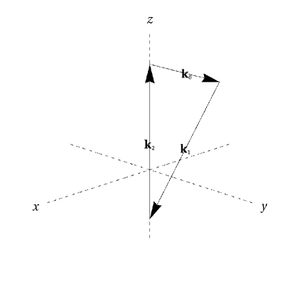
Figure 1: Schematical diagram for illustrating represention of momentums $\textbf{k}_{0}$, $\textbf{k}_{1}$, and $\textbf{k}_{2}$.

In this representation, the polarization vectors for momentums $\textbf{k}_{i}$ are given by

$$e_{1}\left(\textbf{k}_{2}\right) = \hat{x}\leavevmode\nobreak\ ,$$ (23a)

$$e_{1}\left(\textbf{k}_{1}\right) = \hat{x}\cos\theta_{k}-\hat{z}\sin\theta_{k}\leavevmode\nobreak\ ,$$ (23b)

$$e_{1}\left(\textbf{k}_{0}\right) = \hat{x}\cos\theta_{k}^{\prime}+\hat{z}\sin\theta_{k}^{\prime}\leavevmode\nobreak\ ,$$ (23c)

$$e_{2}\left(\textbf{k}_{2}\right) = e_{2}\left(\textbf{k}_{1}\right)=e_{2}\left(\textbf{k}_{0}\right)=\hat{y}\leavevmode\nobreak\ ,$$ (23d)

where $\theta_{k}^{\prime}\equiv\arccos\left(\widehat{\textbf{k}}_{2}\cdot\widehat{\textbf{k}}_{0}\right)=\arccos\left(\widehat{\textbf{k}}_{2}\cdot\left(-\textbf{k}_{1}-\textbf{k}_{2}\right)\left|\textbf{k}_{1}+\textbf{k}_{2}\right|^{-1}\right)$. Therefore, we can obtain the polarization tensors with

$$e^{+}\left(\textbf{k}_{i}\right) \equiv \frac{1}{\sqrt{2}}\left(e_{1}\left(\textbf{k}_{i}\right)\otimes e_{1}\left(\textbf{k}_{i}\right)-e_{2}\left(\textbf{k}_{i}\right)\otimes e_{2}\left(\textbf{k}_{i}\right)\right)\leavevmode\nobreak\ ,$$ (24a)

$$e^{\times}\left(\textbf{k}_{i}\right) \equiv \frac{1}{\sqrt{2}}\left(e_{1}\left(\textbf{k}_{i}\right)\otimes e_{2}\left(\textbf{k}_{i}\right)+e_{1}\left(\textbf{k}_{i}\right)\otimes e_{2}\left(\textbf{k}_{i}\right)\right)\leavevmode\nobreak\ .$$ (24b)

Utilizing the polariztion tensors in Eq. (24), the explict expression of $\mathbb{P}^{\lambda_{0}\lambda_{1}\lambda_{2}}$ is obtained and presented in Appendix C.

As the bispectrum in Eq. (16) replies on the dynamics of SIGWs, in the subsequent parts, we will calculate the bispectrum for the matter-dominated era and the radiation-dominated era, separately.

III.2.1 Bispectrum of SIGWs generated during matter-dominated era

For the matter-dominated era, the kernel function given in Eq. (6) is independent of momentum p. Thus the bispectrum in Eq. (16) can be rewritten as

$$B^{\lambda_{0}\lambda_{1}\lambda_{2}}\left(\textbf{k}_{1},\textbf{k}_{2}\right) = 4I_{h}^{({\rm MD})}\left(\left|\textbf{k}_{1}+\textbf{k}_{2}\right|,\eta\right)I_{h}^{({\rm MD})}(k_{1},\eta)I_{h}^{({\rm MD})}(k_{2},\eta)$$ (25)

$$\times\int\frac{{\rm d}^{3}p}{(2\pi)^{3}}\left\{P_{\Psi}\left(\left|\textbf{k}_{2}-\textbf{p}\right|\right)P_{\Psi}\left(\left|\textbf{k}_{1}+\textbf{k}_{2}-\textbf{p}\right|\right)P_{\Psi}(p)\mathbb{P}^{\lambda_{0}\lambda_{1}\lambda_{2}}\right\}\leavevmode\nobreak\ .$$

At the late time $\eta\rightarrow\infty$, the kernel function $I_{h}^{({\rm MD})}$ tends to be a constant. It might suggest that the non-Gaussianity of SIGWs here could remain at the late time. We will further address it in Sec. IV. To compute the bispectrum in Eq. (25), we would utilize $\mathbb{P}^{\lambda_{0}\lambda_{1}\lambda_{2}}$ presented in Appendix C. Besides, we also adopt a phenomenological approach by considering the lognormal curvature spectrum as follows,

$$\mathcal{P}_{\Psi}(k) = \frac{A}{\sqrt{2\pi}\Delta}e^{-\frac{1}{2\Delta^{2}}\left(\ln\left(\frac{k}{k_{\ast}}\right)\right)^{2}}\leavevmode\nobreak\ .$$ (26)

The curvature power spectrum has a peak at $k_{*}$ with the width of $\Delta$. As shown in Eq. (9), the dimensionless power spectrum is related to the power spectrum through $\mathcal{P}_{\Psi}(k)=k^{3}(2\pi^{2})^{-1}P_{\Psi}(k)$.

Here, we calculate the bispectrum numerically. It is found that the polarization components, $\times\times\times$, $++\times$, $+\times+$, and $\times++$ are much smaller than the rest of the components over three orders of magnitude. Thus we would ignore them in this study. Associating the numerical results with Eq. (16), we obtain $B_{h}^{+++}(\textbf{k}_{1},\textbf{k}_{2})=B_{h}^{+++}(\textbf{k}_{2},\textbf{k}_{1})$, $B_{h}^{+\times\times}(\textbf{k}_{1},\textbf{k}_{2})=B_{h}^{+\times\times}(\textbf{k}_{2},\textbf{k}_{1})$, and $B_{h}^{++\times}(\textbf{k}_{1},\textbf{k}_{2})=B_{h}^{+\times+}(\textbf{k}_{2},\textbf{k}_{1})$. We also show the bispectrum as function of $k_{1}$ and $k_{2}$ for selected width $\Delta$ in Figs. 2 and 3. The bispectrum could be positive or negative, which are denoted as solid and dashed curves in the bottom panels. The maximum absolute value of the bispectrum amplitude decreases with width of the curvature power spectrum. It suggests that the peaked curvature power spectrum can enhance the bispectrum amplitude. Comparing between Figs. 2 and 3, the absolute value of the bispectrum with $\theta_{k}=5\pi/6$ has a smaller plateau than that for $\theta_{k}=\pi/6$.

Figure 2: Top panel: $+++$ component of the dimensionless bispectrum as function of $k_{1}/k_{*}$ and $k_{2}/k_{*}$. Bottom panel: $+++$ component of the dimensionless bispectrum as function of $k_{2}/k_{*}$ for given $k_{1}/k_{*}$. In these plots, we have fixed $\theta_{k}=\pi/6$ and $k_{*}\eta=100$ and considered the width of the curvature power spectrum $\Delta=1/2$ (left panel), 1 (medium panel), and $2$ (right panel), respectively.

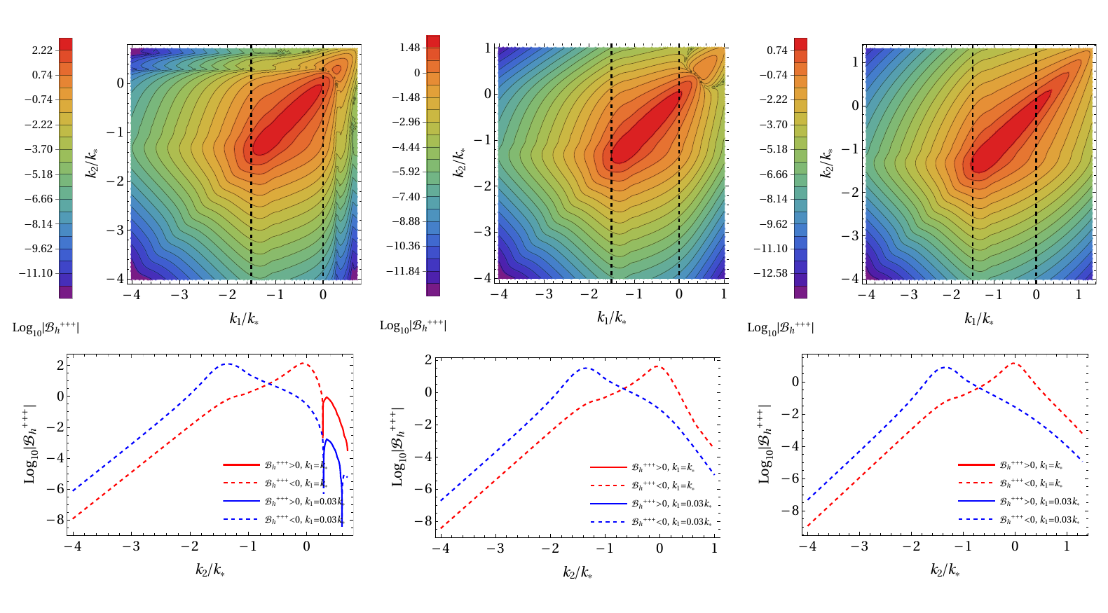
Figure 3: Top panel: $+++$ component of the dimensionless bispectrum as function of $k_{1}/k_{*}$ and $k_{2}/k_{*}$. Bottom panel: $+++$ component of the dimensionless bispectrum as function of $k_{2}/k_{*}$ for given $k_{1}/k_{*}$. In these plots, we have fixed $\theta_{k}=5\pi/6$ and $k_{*}\eta=100$, and considered the width of the curvature power spectrum $\Delta=1/2$ (left panel), $1$ (medium panel), and $2$ (right panel), respectively.

Fig. 4 shows the bispectrum as function of $k_{1}$ and $k_{1}$ for selected $k_{*}\eta$. The plateau of the bispectrum increases with $k_{*}\eta$.

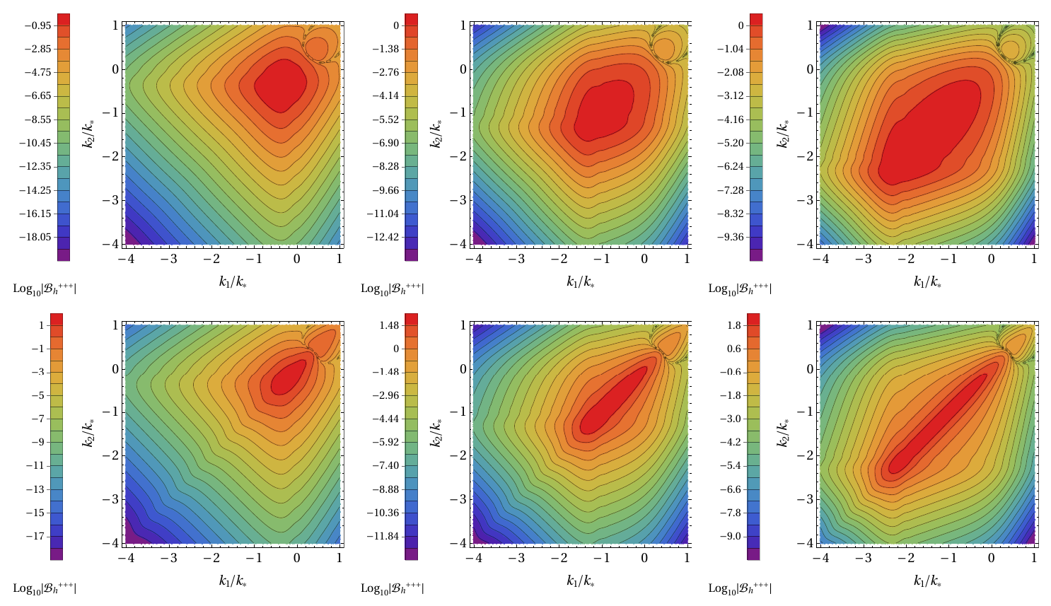
Figure 4: $+++$ component of the dimensionless bispectrum as function of $k_{1}/k_{*}$ and $k_{2}/k_{*}$ for $k_{*}\eta=10$ (left panels), $100$ (medium panels), and $1000$ (right panels), respectively. In theses plots, we have fixed the width $\Delta=1$, and $\theta_{k}=\pi/6$ (top panels) and $\theta_{k}=5\pi/6$ (bottom panels).

Fig. 5 shows the bispectrum as function of $k_{2}$ for selected $k_{1}$ and $\theta_{k}$. The peaks of the bispectrum become narrower as $\theta_{k}$ increases. To further show the relation between the bispectrum amplitude and the $\theta_{k}$, we present the bispectrum as function of $\theta_{k}$ for given $k_{1}$ and $k_{2}$ in Fig. 6. For $k_{1}$ and $k_{2}$ located on the plateau as shown in Fig. 4, the absolute value of bispectrum amplitudes monotonically increases with $\theta_{k}$. In other cases, the bispectrum amplitudes are suppressed as $\theta_{k}\rightarrow 0$ or $\theta_{k}\rightarrow\pi$. The same conclusion holds for different polarization components, namely $\times\times+$, $+\times\times$, and $+++$.

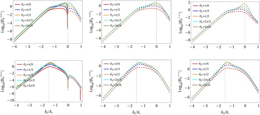
Figure 5: The dimensionless bispectrum as function of $k_{2}/k_{*}$ for selected $\theta_{k}$ with fixed $k_{1}/k_{*}=1$ (top panels) and $k_{1}/k_{*}=10^{-1.5}$ (bottom panels). In these plots, we consider the width $\Delta=1$ and $k_{*}\eta=100$.

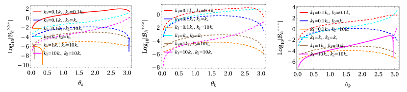
Figure 6: The dimensionless bispectrum as function of $\theta_{k}$ for selected $k_{2}/k_{*}$ and $k_{1}/k_{*}$. In these plots, we consider the width $\Delta=1$ and $k_{*}\eta=100$.

III.2.2 Bispectrum of SIGWs generated during radination-dominated era

In the radiation-dominated era, we are interested in the bispectrum at the late time limit $\eta\rightarrow\infty$ because it might correspond to SGWB that we observe Kohri and Terada (2018). In this case, the kernel function at the late time was presented in Eq. (4). By substituting the kernel function into the bispectrum given in Eq. (16), it is found that the oscillation average should be employed for further computation, and finally we obtain

$$B^{\lambda_{0}\lambda_{1}\lambda_{2}}\left(\textbf{k}_{1},\textbf{k}_{2}\right) = \Delta_{\eta}\left[k_{1}+k_{2}-\left|\textbf{k}_{1}+\textbf{k}_{2}\right|\right]B^{\lambda_{0}\lambda_{1}\lambda_{2}}_{0}\left(\textbf{k}_{1},\textbf{k}_{2}\right)$$ (27)

$$+\Delta_{\eta}\left[\left|\textbf{k}_{1}+\textbf{k}_{2}\right|-k_{1}+k_{2}\right]B^{\lambda_{0}\lambda_{1}\lambda_{2}}_{+}\left(\textbf{k}_{1},\textbf{k}_{2}\right)$$

$$+\Delta_{\eta}\left[\left|\textbf{k}_{1}+\textbf{k}_{2}\right|+k_{1}-k_{2}\right]B^{\lambda_{0}\lambda_{1}\lambda_{2}}_{-}\left(\textbf{k}_{1},\textbf{k}_{2}\right)\leavevmode\nobreak\ ,$$

where the $\Delta_{\eta}[\ast]$ is defined within the framework of the oscillation average scheme in Appendix A, and

$$B_{*}^{\lambda_{0}\lambda_{1}\lambda_{2}}\left(\textbf{k}_{1},\textbf{k}_{2}\right)=\frac{1}{\left|\textbf{k}_{1}+\textbf{k}_{2}\right|\left|\textbf{k}_{1}\right|\left|\textbf{k}_{2}\right|\eta^{3}}\int\frac{{\rm d}^{3}p}{(2\pi)^{3}}\left\{P_{\Psi}\left(\left|\textbf{k}_{2}-\textbf{p}\right|\right)P_{\Psi}\left(\left|\textbf{k}_{1}+\textbf{k}_{2}-\textbf{p}\right|\right)P_{\Psi}(p)\mathbb{P}^{\lambda_{0}\lambda_{1}\lambda_{2}}I_{*}\right\}\leavevmode\nobreak\ ,$$

(28)

and the $I_{*}$ with $*=0,\pm$ can be expressed in terms of the kernel functions in Eq. (5), namely

$$I_{0} \equiv I_{A}\left(\left|\textbf{k}_{1}+\textbf{k}_{2}-\textbf{p}\right|,p,\left|\textbf{k}_{1}+\textbf{k}_{2}\right|\right)I_{A}\left(\left|\textbf{k}_{1}+\textbf{k}_{2}-\textbf{p}\right|,\left|\textbf{k}_{2}-\textbf{p}\right|,k_{1}\right)I_{A}\left(\left|\textbf{k}_{2}-\textbf{p}\right|,p,k_{2}\right)$$ (29a)

$$-I_{A}\left(\left|\textbf{k}_{1}+\textbf{k}_{2}-\textbf{p}\right|,p,\left|\textbf{k}_{1}+\textbf{k}_{2}\right|\right)I_{B}\left(\left|\textbf{k}_{1}+\textbf{k}_{2}-\textbf{p}\right|,\left|\textbf{k}_{2}-\textbf{p}\right|,k_{1}\right)I_{B}\left(\left|\textbf{k}_{2}-\textbf{p}\right|,p,k_{2}\right)$$

$$+I_{B}\left(\left|\textbf{k}_{1}+\textbf{k}_{2}-\textbf{p}\right|,p,\left|\textbf{k}_{1}+\textbf{k}_{2}\right|\right)I_{A}\left(\left|\textbf{k}_{1}+\textbf{k}_{2}-\textbf{p}\right|,\left|\textbf{k}_{2}-\textbf{p}\right|,k_{1}\right)I_{B}\left(\left|\textbf{k}_{2}-\textbf{p}\right|,p,k_{2}\right)$$

$$+I_{B}\left(\left|\textbf{k}_{1}+\textbf{k}_{2}-\textbf{p}\right|,p,\left|\textbf{k}_{1}+\textbf{k}_{2}\right|\right)I_{B}\left(\left|\textbf{k}_{1}+\textbf{k}_{2}-\textbf{p}\right|,\left|\textbf{k}_{2}-\textbf{p}\right|,k_{1}\right)I_{A}\left(\left|\textbf{k}_{2}-\textbf{p}\right|,p,k_{2}\right)\leavevmode\nobreak\ ,$$

$$I_{\pm} \equiv I_{A}\left(\left|\textbf{k}_{1}+\textbf{k}_{2}-\textbf{p}\right|,p,\left|\textbf{k}_{1}+\textbf{k}_{2}\right|\right)I_{A}\left(\left|\textbf{k}_{1}+\textbf{k}_{2}-\textbf{p}\right|,\left|\textbf{k}_{2}-\textbf{p}\right|,k_{1}\right)I_{A}\left(\left|\textbf{k}_{2}-\textbf{p}\right|,p,k_{2}\right)$$ (29b)

$$+I_{A}\left(\left|\textbf{k}_{1}+\textbf{k}_{2}-\textbf{p}\right|,p,\left|\textbf{k}_{1}+\textbf{k}_{2}\right|\right)I_{B}\left(\left|\textbf{k}_{1}+\textbf{k}_{2}-\textbf{p}\right|,\left|\textbf{k}_{2}-\textbf{p}\right|,k_{1}\right)I_{B}\left(\left|\textbf{k}_{2}-\textbf{p}\right|,p,k_{2}\right)$$

$$\mp I_{B}\left(\left|\textbf{k}_{1}+\textbf{k}_{2}-\textbf{p}\right|,p,\left|\textbf{k}_{1}+\textbf{k}_{2}\right|\right)I_{A}\left(\left|\textbf{k}_{1}+\textbf{k}_{2}-\textbf{p}\right|,\left|\textbf{k}_{2}-\textbf{p}\right|,k_{1}\right)I_{B}\left(\left|\textbf{k}_{2}-\textbf{p}\right|,p,k_{2}\right)$$

$$\pm I_{B}\left(\left|\textbf{k}_{1}+\textbf{k}_{2}-\textbf{p}\right|,p,\left|\textbf{k}_{1}+\textbf{k}_{2}\right|\right)I_{B}\left(\left|\textbf{k}_{1}+\textbf{k}_{2}-\textbf{p}\right|,\left|\textbf{k}_{2}-\textbf{p}\right|,k_{1}\right)I_{A}\left(\left|\textbf{k}_{2}-\textbf{p}\right|,p,k_{2}\right)\leavevmode\nobreak\ .$$

It is found that the bispectrum is of flattened-type non-Gaussianity for a large and finite $\eta$. As shown in Appendix A, we have $\lim_{\eta\rightarrow\infty}\Delta_{\eta}[*]=0$ for the triangular bispectrum. It might be understood that the time oscillations can suppress the bispectrum amplitudes.

For illustration, we can let $k_{1}+k_{2}-\left|\textbf{k}_{1}+\textbf{k}_{2}\right|\equiv\epsilon/\eta$ and $0<\epsilon\ll 1$, for example. In this scenario, the configuration for describing the flattened-type non-Gaussianity is presented in Tab. 1.

Table 1: The flattened bispectrum of SIGWs generated in radiation-dominated era

Bispectra	Length relation	$\theta_{k,\rm min/max}$	allowed $k_{1}$, $k_{2}$	Bispectra shape
$B^{\lambda_{0}\lambda_{1}\lambda_{2}}_{0}$	$k_{1}+k_{2}-\left|\textbf{k}_{1}+\textbf{k}_{2}\right|=\epsilon/\eta$	$\sqrt{\left(\frac{k_{2}}{k_{1}}+1\right)\frac{2\epsilon}{k_{2}\eta}}$	/
$B^{\lambda_{0}\lambda_{1}\lambda_{2}}_{\pm}$	$\left|\textbf{k}_{1}+\textbf{k}_{2}\right|\pm(k_{2}-k_{1})=\epsilon/\eta$	$\pi-\sqrt{\left|\frac{k_{2}}{k_{1}}-1\right|\frac{2\epsilon}{k_{2}\eta}}$	$\pm(k_{1}-k_{2})>0$

In subsequent calculations, we prefer to quantify the flattened non-Gaussianity with a single parameter $\theta_{k}$. Hence, we can futher evaluate Eq. (28) by expanding the expression at the $\theta_{k}\rightarrow 0$ for $B_{0}^{\lambda_{0}\lambda_{1}\lambda_{2}}$, namely,

$$B_{0}^{\lambda_{0}\lambda_{1}\lambda_{2}}\left(\textbf{k}_{1},\textbf{k}_{2}\right) \simeq \frac{\theta_{k}^{2}}{(k_{1}+k_{2})k_{1}k_{2}\eta^{3}}\int\frac{{\rm d}^{3}p}{(2\pi)^{3}}\Big{\{}P_{\Psi}\left(\left|\textbf{k}_{2}-\textbf{p}\right|\right)P_{\Psi}\left(\left|(k_{1}+k_{2})\widehat{\textbf{k}}_{2}-\textbf{p}\right|\right)P_{\Psi}(p)\mathbb{B}_{1}$$ (30)

$$+P_{\Psi}\left(\left|\textbf{k}_{2}-\textbf{p}\right|\right)P_{\Psi}^{\prime}\left(\left|\left(k_{1}+k_{2}\right)\widehat{\textbf{k}}_{2}-\textbf{p}\right|\right)P_{\Psi}(p)\bar{\mathbb{B}}_{1}$$

$$+P_{\Psi}\left(\left|\textbf{k}_{2}-\textbf{p}\right|\right)P_{\Psi}^{\prime\prime}\left(\left|(k_{1}+k_{2})\widehat{\textbf{k}}_{2}-\textbf{p}\right|\right)P_{\Psi}(p)\tilde{\mathbb{B}}_{1}\Big{\}}\leavevmode\nobreak\ ,$$

where the $P^{\prime}_{\Psi}(k)$ and $P_{\Psi}^{\prime\prime}(k)$ are the derivative with respect to $k$, and

$$\mathbb{B}_{0} = \frac{1}{2}\left.\frac{\partial^{2}\mathbb{P}^{\lambda_{0}\lambda_{1}\lambda_{2}}}{\partial\theta_{k}^{2}}\right|_{\theta_{k}=0}I_{0}|_{\theta_{k}=0}-\frac{k_{1}p\cos\phi\sin\phi}{\left|(k_{1}+k_{2})\widehat{\textbf{k}}_{2}-\textbf{p}\right|}\left.\frac{\partial\mathbb{P}^{\lambda_{0}\lambda_{1}\lambda_{2}}}{\partial\theta_{k}}\right|_{\theta_{k}=0}\left.\frac{\partial I_{0}}{\partial\left|\textbf{k}_{1}+\textbf{k}_{2}-\textbf{p}\right|}\right|_{\theta_{k}=0}$$ (31a)

$$+\frac{k_{1}^{2}p^{2}\cos^{2}\phi\sin^{2}\theta\mathbb{P}^{\lambda_{0}\lambda_{1}\lambda_{2}}|_{\theta_{k}=0}}{2\left|(k_{1}+k_{2})\widehat{\textbf{k}}_{2}-\textbf{p}\right|^{3}}\Bigg{(}\left|(k_{1}+k_{2})\widehat{\textbf{k}}_{2}-\textbf{p}\right|\left.\frac{\partial^{2}I_{0}}{\partial\left|\textbf{k}_{1}+\textbf{k}_{2}-\textbf{p}\right|^{2}}\right|_{\theta_{k}=0}$$

$$-\left.\frac{\partial I_{0}}{\partial\left|\textbf{k}_{1}+\textbf{k}_{2}-\textbf{p}\right|}\right|_{\theta_{k}=0}\Bigg{)}\leavevmode\nobreak\ ,$$

$$\bar{\mathbb{B}}_{0} = -\frac{k_{1}p\cos\phi\sin\theta}{\left|(k_{1}+k_{2})\widehat{\textbf{k}}_{2}-\textbf{p}\right|}\left.\frac{\partial\mathbb{P}^{\lambda_{0}\lambda_{1}\lambda_{2}}}{\partial\theta_{k}}\right|_{\theta_{k}=0}I_{0}|_{\theta_{k}=0}$$

$$+\frac{k_{1}^{2}p^{2}\cos^{2}\phi\sin^{2}\theta\mathbb{P}^{\lambda_{0}\lambda_{1}\lambda_{2}}|_{\theta_{k}=0}}{2\left|(k_{1}+k_{2})\widehat{\textbf{k}}_{2}-\textbf{p}\right|^{3}}\left(2\left|(k_{1}+k_{2})\widehat{\textbf{k}}_{2}-\textbf{p}\right|\left.\frac{\partial I_{0}}{\partial\left|\textbf{k}_{1}+\textbf{k}_{2}-\textbf{p}\right|}\right|_{\theta_{k}=0}-I_{0}|_{\theta_{k}=0}\right)\leavevmode\nobreak\ ,$$

$$\tilde{\mathbb{B}}_{0} = \frac{k_{1}^{2}p^{2}\cos^{2}\phi\sin^{2}\theta\mathbb{P}^{\lambda_{0}\lambda_{1}\lambda_{2}}|_{\theta_{k}=0}I_{0}|_{\theta_{k}=0}}{2\left|(k_{1}+k_{2})\widehat{\textbf{k}}_{2}-\textbf{p}\right|^{2}}\leavevmode\nobreak\ .$$ (31c)

Similarly, we expand $B_{\pm}^{\lambda_{0}\lambda_{1}\lambda_{2}}$ at the $\theta_{k}=\pi$, namely,

$$B_{\pm}^{\lambda_{0}\lambda_{1}\lambda_{2}}\left(\textbf{k}_{1},\textbf{k}_{2}\right) \simeq \frac{(\theta_{k}-\pi)^{2}}{|k_{2}-k_{1}|k_{1}k_{2}\eta^{3}}\int\frac{{\rm d}^{3}p}{(2\pi)^{3}}\Big{\{}P_{\Psi}\left(\left|\textbf{k}_{2}-\textbf{p}\right|\right)P_{\Psi}\left(\left|(k_{2}-k_{1})\widehat{\textbf{k}}_{2}-\textbf{p}\right|\right)P_{\Psi}(p)\mathbb{B}_{i}$$ (32)

$$+P_{\Psi}\left(\left|\textbf{k}_{2}-\textbf{p}\right|\right)P_{\Psi}^{\prime}\left(\left|\left(k_{2}-k_{1}\right)\widehat{\textbf{k}}_{2}-\textbf{p}\right|\right)P_{\Psi}(p)\bar{\mathbb{B}}_{i}$$

$$+P_{\Psi}\left(\left|\textbf{k}_{2}-\textbf{p}\right|\right)P_{\Psi}^{\prime\prime}\left(\left|(k_{2}-k_{1})\widehat{\textbf{k}}_{2}-\textbf{p}\right|\right)P_{\Psi}(p)\tilde{\mathbb{B}}_{i}\Big{\}}\leavevmode\nobreak\ ,$$

where

$$\mathbb{B}_{\pm} = \frac{1}{2}\left.\frac{\partial^{2}\mathbb{P}^{\lambda_{0}\lambda_{1}\lambda_{2}}}{\partial\theta_{k}^{2}}\right|_{\theta_{k}=\pi}I_{\pm}|_{\theta_{k}=\pi}+\frac{k_{1}p\cos\phi\sin\phi}{\left|(k_{2}-k_{1})\widehat{\textbf{k}}_{2}-\textbf{p}\right|}\left.\frac{\partial\mathbb{P}^{\lambda_{0}\lambda_{1}\lambda_{2}}}{\partial\theta_{k}}\right|_{\theta_{k}=\pi}\left.\frac{\partial I_{\pm}}{\partial\left|\textbf{k}_{1}+\textbf{k}_{2}-\textbf{p}\right|}\right|_{\theta_{k}=\pi}$$ (33a)

$$+\frac{k_{1}^{2}p^{2}\cos^{2}\phi\sin^{2}\theta\mathbb{P}^{\lambda_{0}\lambda_{1}\lambda_{2}}|_{\theta_{k}=0}}{2\left|(k_{2}-k_{1})\widehat{\textbf{k}}_{2}-\textbf{p}\right|^{3}}\Bigg{(}\left|(k_{2}-k_{1})\widehat{\textbf{k}}_{2}-\textbf{p}\right|\left.\frac{\partial^{2}I_{\pm}}{\partial\left|\textbf{k}_{1}+\textbf{k}_{2}-\textbf{p}\right|^{2}}\right|_{\theta_{k}=\pi}$$

$$-\left.\frac{\partial I_{\pm}}{\partial\left|\textbf{k}_{1}+\textbf{k}_{2}-\textbf{p}\right|}\right|_{\theta_{k}=\pi}\Bigg{)}\leavevmode\nobreak\ ,$$

$$\bar{\mathbb{B}}_{\pm} = \frac{k_{1}p\cos\phi\sin\theta}{\left|(k_{2}-k_{1})\widehat{\textbf{k}}_{2}-\textbf{p}\right|}\left.\frac{\partial\mathbb{P}^{\lambda_{0}\lambda_{1}\lambda_{2}}}{\partial\theta_{k}}\right|_{\theta_{k}=\pi}I_{\pm}|_{\theta_{k}=\pi}$$

$$+\frac{k_{1}^{2}p^{2}\cos^{2}\phi\sin^{2}\theta\mathbb{P}^{\lambda_{0}\lambda_{1}\lambda_{2}}|_{\theta_{k}=\pi}}{2\left|(k_{2}-k_{1})\widehat{\textbf{k}}_{2}-\textbf{p}\right|^{3}}\Bigg{(}2\left|(k_{2}-k_{1})\widehat{\textbf{k}}_{2}-\textbf{p}\right|\left.\frac{\partial I_{\pm}}{\partial\left|\textbf{k}_{1}+\textbf{k}_{2}-\textbf{p}\right|}\right|_{\theta_{k}=\pi}-I_{\pm}|_{\theta_{k}=\pi}\Bigg{)}\leavevmode\nobreak\ ,$$

$$\tilde{\mathbb{B}}_{\pm} = \frac{k_{1}^{2}p^{2}\cos^{2}\phi\sin^{2}\theta\mathbb{P}^{\lambda_{0}\lambda_{1}\lambda_{2}}|_{\theta_{k}=\pi}I_{\pm}|_{\theta_{k}=\pi}}{2\left|(k_{2}-k_{1})\widehat{\textbf{k}}_{2}-\textbf{p}\right|^{2}}\leavevmode\nobreak\ .$$ (33c)

Due to the integration over the coordinate $\phi$, the leading orders of the bispectra are shown to be proportional to the $\theta_{k}^{2}$ in Eq. (30) and $(\pi-\theta_{k})^{2}$ in Eq. (32). However, it is not as simple as expected. It is found that the expansion at $\theta_{k}\rightarrow 0$ or $\pi$ introduce singularities in the terms of $\partial^{2}I_{*}/\partial\left|\textbf{k}_{1}+\textbf{k}_{2}-\textbf{p}\right|_{\theta_{k}=0,\pi}$, thereby leading to the integrals to be devergent. To obtain correct integrations, the regularization scheme should be employed as presented in Appendix B. With the regularization scheme, it is noted that the regularized singular terms would dominate the bispectrum amplitudes and result in the bispectrum proportional to $\theta_{k}^{\beta}$ or $(\pi-\theta_{k})^{\beta}$, where $\beta<2$. This feature is extensively illustrated in Appendix B. Here, in this sense, the leading orders of the expansions in Eqs. (30) and (32) can reduce to

$$B_{0}^{\lambda_{0}\lambda_{1}\lambda_{2}}\left(\textbf{k}_{1},\textbf{k}_{2}\right) \simeq \frac{\theta_{k}^{2}}{(k_{1}+k_{2})k_{1}k_{2}\eta^{3}}\int\frac{{\rm d}^{3}p}{(2\pi)^{3}}\Bigg{\{}P_{\Psi}\left(\left|\textbf{k}_{2}-\textbf{p}\right|\right)P_{\Psi}\left(\left|(k_{1}+k_{2})\widehat{\textbf{k}}_{2}-\textbf{p}\right|\right)P_{\Psi}(p)\bar{\mathbb{P}}^{\lambda_{0}\lambda_{1}\lambda_{2}}_{0}$$

$$\times\frac{p^{8}\sin^{8}\theta}{64\sqrt{2}k_{2}^{2}(k_{1}+k_{2})^{2}((k_{1}+k_{2})^{2}+p^{2}-2(k_{1}+k_{2})p\cos\theta)}\left.\frac{\partial^{2}I_{0}}{\partial\left|\textbf{k}_{1}+\textbf{k}_{2}-\textbf{p}\right|^{2}}\right|_{\theta_{k}=0}\Bigg{\}}\leavevmode\nobreak\ ,$$

$$B_{\pm}^{\lambda_{0}\lambda_{1}\lambda_{2}}\left(\textbf{k}_{1},\textbf{k}_{2}\right) \simeq \frac{(\theta_{k}-\pi)^{2}}{|k_{2}-k_{1}|k_{1}k_{2}\eta^{3}}\int\frac{{\rm d}^{3}p}{(2\pi)^{3}}\Bigg{\{}P_{\Psi}\left(\left|\textbf{k}_{2}-\textbf{p}\right|\right)P_{\Psi}\left(\left|(k_{2}-k_{1})\widehat{\textbf{k}}_{2}-\textbf{p}\right|\right)P_{\Psi}(p)\bar{\mathbb{P}}^{\lambda_{0}\lambda_{1}\lambda_{2}}_{\pm}$$

$$\times\frac{p^{8}\sin^{8}\theta}{64\sqrt{2}k_{2}^{2}(k_{2}-k_{1})^{2}((k_{2}-k_{1})^{2}+p^{2}-2(k_{2}-k_{1})p\cos\theta)}\left.\frac{\partial^{2}I_{\pm}}{\partial\left|\textbf{k}_{1}+\textbf{k}_{2}-\textbf{p}\right|^{2}}\right|_{\theta_{k}=\pi}\Bigg{\}}\leavevmode\nobreak\ ,$$

where $\bar{\mathbb{P}}^{\lambda_{0}\lambda_{1}\lambda_{2}}_{\ast}$ is defined in Tab. 2. The $\bar{\mathbb{P}}^{\lambda_{0}\lambda_{1}\lambda_{2}}$ with constant components indicates that the polarization components differ only in bispectrum amplitudes. Based on the regularization scheme presented in Appendix B, we introduce regularization parameters $\varepsilon_{0}$ and $\varepsilon_{\pi}$. It can result in $\sqrt{\varepsilon_{0}}B_{0}^{\lambda_{0}\lambda_{1}\lambda_{2}}$ and $\sqrt{\varepsilon_{\pi}}B_{\pm}^{\lambda_{0}\lambda_{1}\lambda_{2}}$ yielding finite values. Here, we ansatz $\varepsilon_{0}=\varepsilon_{\pi}\equiv\varepsilon$ for the sake of simplicity.

Table 2:

$\lambda_{0}\lambda_{1}\lambda_{2}$	$\bar{\mathbb{P}}_{0}$	$\bar{\mathbb{P}}_{+}$	$\bar{\mathbb{P}}_{-}$
××+	$-1$	$-1$	$1$
×+×	$-1$	$1$	$-1$
+××	$1$	$-1$	$-1$
+++	3	3	3
others	0	0	0

Associating the results in Tab. 2 with Eq. (16), we can also obtain

$$B_{h}^{\times\times+}(k_{1},k_{2},\theta_{k}\rightarrow 0)=B_{h}^{\times+\times}(k_{2},k_{1},\theta_{k}\rightarrow 0) = -\frac{1}{3}(B_{0}^{+++}(k_{1},k_{2})+B_{0}^{+++}(k_{2},k_{1}))\leavevmode\nobreak\ ,$$ (35a)

$$B_{h}^{+++}(k_{1},k_{2},\theta_{k}\rightarrow 0)=3B_{h}^{\times++}(k_{1},k_{2},\theta_{k}\rightarrow 0) = B_{0}^{+++}(k_{1},k_{2})+B_{0}^{+++}(k_{2},k_{1})\leavevmode\nobreak\ ,$$ (35b)

and

$$B_{h}^{\times\times+}(k_{1},k_{2},\theta_{k}\rightarrow\pi)=B_{h}^{\times+\times}(k_{2},k_{1},\theta_{k}\rightarrow\pi) = \frac{1}{3}(B_{\pm}^{+++}(k_{1},k_{2})+B_{\pm}^{+++}(k_{2},k_{1}))$$ (35c)

$$\times(\Theta(k_{2}-k_{1})-\Theta(k_{1}-k_{2}))\leavevmode\nobreak\ ,$$

$$B_{h}^{+++}(k_{1},k_{2},\theta_{k}\rightarrow\pi)=3B_{h}^{\times++}(k_{1},k_{2},\theta_{k}\rightarrow\pi) = B_{\pm}^{+++}(k_{1},k_{2})+B_{\pm}^{+++}(k_{2},k_{1})\leavevmode\nobreak\ ,$$ (35d)

where the $\Theta(x)$ is Heaviside step function. It shows that the different polarization components of the bispectrum $B_{h}^{\lambda_{0}\lambda_{1}\lambda_{2}}$ can all be derived from two independent quantities, i.e., $B_{0}^{+++}$ and $B_{\pm}^{+++}$.

In the phenomenological approach, we also consider the log-normal curvature power spectrum as given in Eq. (26). Fig. 7 and 8 show the bispectrum as function of $k_{1}$ and $k_{2}$ for selected $\Delta$ with $\theta_{k}\rightarrow 0$ and $\theta_{k}\rightarrow\pi$, respectively. Because of the constant $\bar{\mathbb{P}}^{\lambda_{0}\lambda_{1}\lambda_{2}}_{\ast}$ as mentioned above, we only plot the $+++$ polarization components. The bispectrum amplitude is shown to be enhanced for a narrower width $\Delta$. Compared between Fig. 7 and Fig. 8, the maximum bispctrum amplitudes for $\theta_{k}\simeq\pi$ are much larger than that of $\theta_{k}\rightarrow 0$.

Figure 7: The dimensionless bispectrum at $\theta_{k}\rightarrow 0$ as function of $k_{1}/k_{\ast}$ and $k_{2}/k_{\ast}$ for $\Delta=1/2$ (left panel), 1 (medium panel), $2$ (right panel). Here, we have $\tilde{\mathcal{B}}_{h}^{+++}\equiv(k_{*}\eta)^{3}\theta_{k}^{-2}\sqrt{\varepsilon}{\mathcal{B}}_{h}^{+++}$.

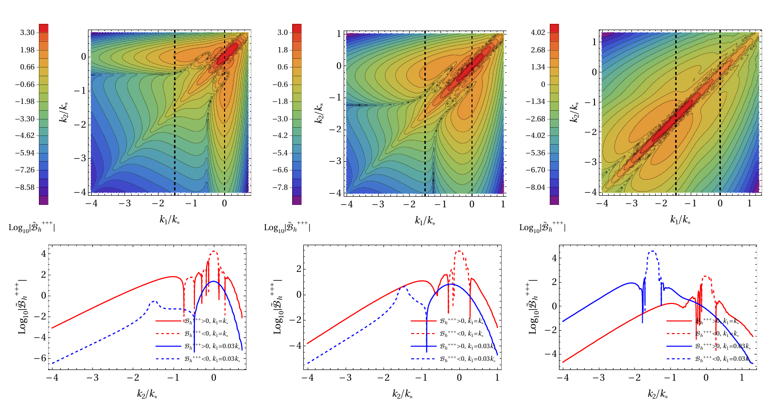
Figure 8: The dimensionless bispectrum at $\theta_{k}\rightarrow\pi$ as function of $k_{1}/k_{\ast}$ and $k_{2}/k_{\ast}$ for $\Delta=1/2$ (left panel), 1 (medium panel), $2$ (right panel). Here, we have $\tilde{\mathcal{B}}_{h}^{+++}\equiv(k_{*}\eta)^{3}\theta_{k}^{-2}\sqrt{\varepsilon}{\mathcal{B}}_{h}^{+++}$.

IV Skewness of the scalar-induced gravitational waves

As mentioned in Sec. II, the degree of non-Gaussianity of SIGWs can be quantified by the skewness. In this section, we wish to examine whether the third-order non-Gaussianity of SIGWs can be ignored. To be specific, whether we have the skewness $|\Gamma|\ll 1$.

Due to the interest in the energy density spectrum of SIGWs, the power spectrum has been completely studied by pioneers Ananda et al. (2007); Baumann et al. (2007); Espinosa et al. (2018); Kohri and Terada (2018); Sasaki et al. (2018); Domènech (2021). By making use of Eqs. (2), (7) and (14), the power spectrum can be given by

$$P_{h}^{\lambda\lambda^{\prime}}\left(\textbf{k}\right) = e^{\lambda}_{ij}\left(\textbf{k}\right)e^{\lambda^{\prime}}_{ab}\left(\textbf{k}\right)\int\frac{{\rm d}^{3}p}{(2\pi)^{3}}\left\{2P_{\Psi}\left(\left|\textbf{k}-\textbf{p}\right|\right)P_{\Psi}\left(\left|\textbf{p}\right|\right)\Theta_{ij}\left(\textbf{k},\textbf{p}\right)\Theta_{ab}\left(\textbf{k},\textbf{p}\right)I_{h}\left(\left|\textbf{k}-\textbf{p}\right|,\left|\textbf{p}\right|,k,\eta\right)^{2}\right\}$$

$$= \frac{1}{2}\delta^{\lambda\lambda^{\prime}}\int\frac{{\rm d}^{3}p}{(2\pi)^{3}}\left\{\left(1-\left(\widehat{\textbf{k}}\cdot\widehat{\textbf{p}}\right)^{2}\right)^{2}\left(\frac{\left|\textbf{p}\right|}{k}\right)^{4}P_{\Psi}\left(\left|\textbf{k}-\textbf{p}\right|\right)P_{\Psi}\left(\left|\textbf{p}\right|\right)I_{h}\left(\left|\textbf{k}-\textbf{p}\right|,\left|\textbf{p}\right|,k,\eta\right)^{2}\right\}\leavevmode\nobreak\ .$$

Therefore, the variance can be obtained by associating the power spectrum in Eq. (LABEL:spectrah) with Eq. (9). We will calculate the skewness by making use of the variances in the matter-dominated era and radiation-dominated era, separately.

Since we have different polarization components for the bispectrum, one can rewrite the skewness in Eq. (13) with polarization indices, namely,

$$\Gamma_{\lambda_{0}\lambda_{1}\lambda_{2}}=\frac{\mu^{3}_{\lambda_{0}\lambda_{1}\lambda_{2}}}{\bar{\sigma}^{3}}\leavevmode\nobreak\ ,$$ (37)

where the average variance is given by $\bar{\sigma}=(\sigma^{++}+\sigma^{\times\times})/2$ based on Eq. (9) and the unpolarized power spectrum given in Eq. (LABEL:spectrah).

We calculate the skewness for SIGWs generated in the matter-dominated era, numerically. The skewness as function of width $\Delta$ is presented in Fig. 9.

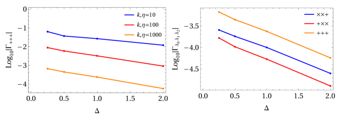
Figure 9: The skewness for SIGWs generated in the matter-dominated era as function of width $\Delta$ of the curvature power spectrum for selected $k_{*}\eta$ (left panel) and different polarizations (right panels).

It is found that the skewness decreases with the width $\Delta$, which indicates that the peaked curvature power spectrum can result in the enhancements of the non-Guassianity of SIGWs. For SIGWs generated from the exit of the inflationary era $\eta=0$ to the $\eta\propto k_{*}^{-1}$, the skewness is shown to be suppressed as the $k_{*}\eta$ increases. Specifically, we have the skewness $\propto(k_{*}\eta)^{-1}$, approximately. It indicates that the non-Guassianity is mostly generated at the time when the perturbations enter the horizon. As SIGWs evolve to the late time with a large $k_{*}\eta$, the superposition of the waves would suppress the non-Gaussianity. In the right panel of Fig. 9, different polarization components of the skewness have similar behavior with respect to the $\Delta$. The $+++$ component of the skewness has the largest amplitude, thereby indicating the largest non-Gaussianity. As suggested by the results in Fig. 9, the skewness is expected to be less than $1$.

In radiation dominated era, the third moments of SIGWs in Eq. (10) reduce to

$$\mu_{\lambda_{0}\lambda_{1}\lambda_{2}}^{3} = \frac{1}{2}\int_{-\infty}^{\infty}{\rm d}\ln k_{1}\int_{-\infty}^{\infty}{\rm d}\ln k_{2}\Bigg{\{}\int_{0}^{\theta_{k,0}}{\rm d}\theta_{k}\{\theta_{k}\mathcal{B}_{h}^{\lambda_{0}\lambda_{1}\lambda_{2}}|_{\theta_{k}\rightarrow 0}\}+\int_{\pi-\theta_{k,\pi}}^{\pi}{\rm d}\theta_{k}\{(\pi-\theta_{k})\mathcal{B}_{h}^{\lambda_{0}\lambda_{1}\lambda_{2}}|_{\theta_{k}\rightarrow\pi}\}\Bigg{\}}$$ (38)

$$= \frac{(k_{\ast}\eta)^{\frac{\nu}{2}-5}}{2(4-\nu)}\int_{-\infty}^{\infty}{\rm d}\ln k_{1}\int_{-\infty}^{\infty}{\rm d}\ln k_{2}\Bigg{\{}\kappa_{0}^{-1}(k_{\ast}\eta)^{3}\theta_{k}^{-2}\sqrt{\varepsilon_{0}}\mathcal{B}_{h}^{\lambda_{0}\lambda_{1}\lambda_{2}}|_{\theta_{k\rightarrow 0}}\left(\left(\frac{k_{2}}{k_{1}}+1\right)\frac{2k_{\ast}}{k_{2}}\right)^{2-\frac{\nu}{2}}$$

$$+\kappa_{\pi}^{-1}(k_{\ast}\eta)^{3}(\pi-\theta_{k})^{-2}\sqrt{\varepsilon_{\pi}}\mathcal{B}_{h}^{\lambda_{0}\lambda_{1}\lambda_{2}}|_{\theta_{k}\rightarrow\pi}\left(\left|\frac{k_{2}}{k_{1}}-1\right|\frac{2k_{\ast}}{k_{2}}\right)^{2-\frac{\nu}{2}}\Bigg{\}}\leavevmode\nobreak\ ,$$

where the $\theta_{k,0}$ and $\theta_{k,\pi}$ are given based on the $\theta_{k,\rm min/max}$ in Tab. 1, namely,

$$\theta_{k,0}\equiv\sqrt{\left(\frac{k_{2}}{k_{1}}+1\right)\frac{2}{k_{2}\eta}}\leavevmode\nobreak\ ,\hskip 14.22636pt\theta_{k,\pi}\equiv\sqrt{\left|\frac{k_{2}}{k_{1}}-1\right|\frac{2}{k_{2}\eta}}\leavevmode\nobreak\ .$$ (39)

By employing the regularization scheme, the integral for the bispectrum $\sqrt{\varepsilon}\mathcal{B}_{h}^{\lambda_{0}\lambda_{1}\lambda_{2}}|_{\theta_{k}\rightarrow 0,\pi}$ is finite. We ansatz $\sqrt{\varepsilon_{0}}=\kappa_{0}\theta_{k}^{\nu}$ and $\sqrt{\varepsilon_{\pi}}=\kappa_{\pi}(\pi-\theta_{k})^{\nu}$, and $0<\nu<2$ in Eq. (38). The upper bound of $\nu$ is determined by the requirement in the colinear limit that the bispectrum must vanish for $\theta_{k}=\pi-\theta_{k}=0$. Because of the poor numerical precision of the integrations, we could not obtain the actual value of $\nu$. Additional discussion on this aspect is provided in Appendix B, where we present an example indicating $\nu\simeq 1.4$. Here, we show the skewness as function of the $\Delta$ with the undetermined parameter $\nu$ in Fig. 10. And we only consider the $+++$ polarization components as the suggestion of Eqs. (35).

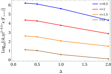
Figure 10: The skewness for SIGWs generated in the radiation-dominated era as function of width $\Delta$ of the curvature power spectrum for selected $\nu$. We have let $\kappa_{0}=\kappa_{\pi}\equiv\kappa$ in the plot.

It also indicates that the non-Gaussianity of SIGWs is enhanced due to the peaked curvature power spectrum. The conclusion remains robust because the monotonicity of function $|\Gamma(\Delta)|$ is independent of the choice of $\nu$. Besides, the skewness of SIGWS also decreases with the $k_{*}\eta$. We can obtain the analytical result of the skewness $\propto(k_{*}\eta)^{\frac{\nu}{2}-2}$. Because of $0<\nu<2$, the non-Gaussinity for SIGWs generated in the radiation-dominated era decays more rapidly with $\eta$ compared to that for the matter-dominated era. Therefore, the skewness is expected to be much less than $1$ due to the substantial value of $k_{*}\eta$ at the late time.

V Conclusions and Discussions

This paper investigated the intrinsic non-Gaussianity of SIGWs, which originate from the non-linear interactions of Einstein’s gravity. In a phenomenological approach, we considered the primordial curvature perturbation modeled as a lognormal spectrum. The bispectrum and skewness of SIGWs generated during the matter-dominated era and the radiation-dominated era were calculated, separately. The bispectrum vanishes in the collinear limit, which is shown to be independent of both the initial conditions and the dynamics of SIGWs. For the SIGWs generated during the radiation-dominated era, the bispectrum is of flatten-type non-Gaussianity, and there are four polarization components $\times\times+$, $\times+\times$, $+\times\times$ and $+++$ left to be non-vanishing. Utilizing the skewness for quantifying the non-Gaussianity, it was found that the curvature power spectrum with a narrow width can result in an enhancement of the third-order non-Gaussianity. The conclusion holds for both the SIGWs generated during the radiation-dominated era and the matter-dominated era.

The decay of non-Gaussianity over time indicates that the accumulation or superposition of waves possesses the capacity to suppress the non-Gaussiananity of SIGWs. It was further found that the third-order non-Gaussianity of SIGWs generated during the radiation-dominated era decays more rapidly over the conformal time compared to that during the matter-dominated era. This can be attributed to the fact that the time oscillations in the radiation-dominated era also serve to suppress the non-Gaussianity of SIGWs.

While there exists no ambiguity in the concept of bispectrum and skewness of SIGWs, obtaining the bispectrum in the case of the radiation-dominated era through a purely numerical approach would be challenging without the time oscillation average scheme and the regularization scheme as presented in this study. The undetermined regularization parameters $\nu$ and $\kappa$ do not affect our main finding regarding the tendency between non-Gaussianity and the width of the curvature power spectrum. To estimate actual values of the regularization parameters, one can refer to the form of $\varepsilon$ presented in the second example of Appendix B, as the singularities both originate from the derivative of kernel functions given in Eq. (5).

The most interesting conclusion of this study lies in the peaked curvature power spectrum can result in an enhancement of the non-Guassianity of SIGWs. It motivates further studies on the non-Gaussinanity of SIGWs with the curvature power spectrum modeled as a delta function. In fact, we have obtained the preliminary results as presented in Appendix D and found it difficult to understand the nature cut-off of the bispectrum. Perhaps, it is expected to be addressed in future studies.

Acknowledgments. This work is supported by the National Nature Science Foundation of China under grant No. 12305073. The author thanks Prof. Sai Wang for useful discussions.

Appendix A Oscillation avarage scheme

For the kernel function at the late time in Eq. (4), the $\cos(k\eta)$ and $\sin(k\eta)$ would be highly oscillated with respect to the $k$ due to a large $\eta$. Here, we proposed an oscillation average scheme via integrating over a period of the trigonometric function, which can be formally given by

$$\underset{x\rightarrow\infty}{{\rm Avg}}\{{\rm trig}(A_{1}x){\rm trig}(A_{2}x)\ldots{\rm trig}(A_{n}x)\} \equiv \frac{A_{1}+A_{2}+\cdots+A_{n}}{2\pi}\int_{x}^{x+\frac{2\pi}{A_{1}+A_{2}+\cdots+A_{n}}}{\rm d}\bar{x}\Big{\{}$$

$${\rm trig}(A_{1}\bar{x}){\rm trig}(A_{2}\bar{x})\ldots{\rm trig}(A_{n}\bar{x})\Big{\}}\leavevmode\nobreak\ ,\leavevmode\nobreak\ \text{for }A_{i}x\gg 1\leavevmode\nobreak\ ,$$

where the $x$ is a large number, and the “${\rm trig}$” represents a trigonometric function, namely, $\cos$ or $\sin$. We strict our attention to the cases that $A_{i}x\gg 1$, because the value of ${\rm trig}(A_{i}x)$ with $A_{i}x\ll 1$ should tend to be a constant, and the oscillation average is deemed unnecessary.

Given that there is a single trigonometric function ${\rm trig}(Ax)$ on the condition that $Ax\gg 1$, one can obtain the oscillation average with

$${\rm Avg}\{\cos(Ax)\}={\rm Avg}\{\sin(Ax)\}=0\leavevmode\nobreak\ .$$ (41)

In the case of $Ax\ll 1$, we have $\cos(Ax)\simeq 1$ and $\sin(Ax)\simeq 0$. It is unnecessary to employ the oscillation average.

For double trigonometric functions in which $Ax$ and $Bx\gg 1$, we can obtain the oscillation averages by making use of Eq. (LABEL:A1), namely,

$${\rm Avg}\{\cos(Ax)\cos(Bx)\} = \frac{A+B}{2\pi(A-B)}\cos\left(\frac{(A-B)\pi}{A+B}+(A-B)x\right)\sin\left(\frac{A-B}{A+B}\pi\right)\leavevmode\nobreak\ ,$$ (42a)

$${\rm Avg}\{\cos(Ax)\sin(Bx)\} = -\frac{A+B}{2\pi(A-B)}\sin\left(\frac{(A-B)\pi}{A+B}+(A-B)x\right)\sin\left(\frac{A-B}{A+B}\pi\right)\leavevmode\nobreak\ ,$$ (42b)

$${\rm Avg}\{\sin(Ax)\sin(Bx)\} = \frac{A+B}{2\pi(A-B)}\cos\left(\frac{(A-B)\pi}{A+B}+(A-B)x\right)\sin\left(\frac{A-B}{A+B}\pi\right)\leavevmode\nobreak\ .$$ (42c)

It is noted that $(A-B)x$ may not be a large number. Utilizing Eqs. (42), in the regime where $A-B\ll 1/x$, we derive ${\rm Avg}\{\cos(Ax)\cos(Bx)\}={\rm Avg}\{\sin(Ax)\sin(Bx)\}\simeq 1/2$, and ${\rm Avg}\{\cos(Ax)\sin(Bx)\}=0$. And, in the regime $(A-B)x\gg 1$, the results reduce to the oscillation average for a single trigonometric function, leading to ${\rm Avg}\{\cos(Ax)\cos(Bx)\}={\rm Avg}\{\sin(Ax)\sin(Bx)\}={\rm Avg}\{\cos(Ax)\sin(Bx)\}=0$. These outcomes can be formally rewritten as

$${\rm Avg}\{\cos(Ax)\cos(Bx)\} = \frac{1}{2}\Delta_{x}[A-B]\leavevmode\nobreak\ ,$$ (43a)

$${\rm Avg}\{\cos(Ax)\sin(Bx)\} = 0\leavevmode\nobreak\ ,$$ (43b)

$${\rm Avg}\{\sin(Ax)\sin(Bx)\} = \frac{1}{2}\Delta_{x}[A-B]\leavevmode\nobreak\ ,$$ (43c)

where we introduce a function for illustration, namely,

$$\Delta_{x}[y] \simeq 1,\hskip 15.00002pt\text{for }y\equiv\frac{\epsilon}{x},\text{ and }\epsilon\ll 1\leavevmode\nobreak\ .$$ (44)

In the derivation of the power spectrum of SIGWs, the oscillations averages: $\cos^{2}(k\eta)=\sin^{2}(k\eta)=1/2$ was employed in previous studies, which is consistent with our scheme presented in Eq. (LABEL:A1).

We can also extend the oscillation average for triplet trigonometric functions in which $Ax,Bx$ and $Cx\gg 1$. By making use of Eq. (LABEL:A1), we obtain

$${\rm Avg}\{\cos(Ax)\cos(Bx)\cos(Cx)\} = \frac{A+B+C}{4\pi}\Bigg{(}\frac{\cos\left((A-B-C)\left(\frac{\pi}{A+B+C}+x\right)\right)\sin\left(\frac{(A-B-C)\pi}{A+B+C}\right)}{A-B-C}$$ (45a)

$$+\frac{\cos\left((A+B-C)\left(\frac{\pi}{A+B+C}+x\right)\right)\sin\left(\frac{(A+B-C)\pi}{A+B+C}\right)}{A+B-C}$$

$$+\frac{\cos\left((A-B+C)\left(\frac{\pi}{A+B+C}+x\right)\right)\sin\left(\frac{(A-B+C)\pi}{A+B+C}\right)}{A-B+C}\Bigg{)}\leavevmode\nobreak\ ,$$

$${\rm Avg}\{\cos(Ax)\cos(Bx)\sin(Cx)\} = \frac{A+B+C}{4\pi}\Bigg{(}-\frac{\sin\left((A-B-C)\left(\frac{\pi}{A+B+C}+x\right)\right)\sin\left(\frac{(A-B-C)\pi}{A+B+C}\right)}{A-B-C}$$ (45b)

$$-\frac{\sin\left((A+B-C)\left(\frac{\pi}{A+B+C}+x\right)\right)\sin\left(\frac{(A+B-C)\pi}{A+B+C}\right)}{A+B-C}$$

$$+\frac{\sin\left((A-B+C)\left(\frac{\pi}{A+B+C}+x\right)\right)\sin\left(\frac{(A-B+C)\pi}{A+B+C}\right)}{A-B+C}\Bigg{)}\leavevmode\nobreak\ ,$$

$${\rm Avg}\{\cos(Ax)\sin(Bx)\sin(Cx)\} = \frac{A+B+C}{4\pi}\Bigg{(}\frac{\cos\left((A+B-C)\left(\frac{\pi}{A+B+C}+x\right)\right)\sin\left(\frac{(A+B-C)\pi}{A+B+C}\right)}{A+B-C}$$ (45c)

$$+\frac{\cos\left((A-B+C)\left(\frac{\pi}{A+B+C}+x\right)\right)\sin\left(\frac{(A-B+C)\pi}{A+B+C}\right)}{A-B+C}$$

$$-\frac{\cos\left((A-B-C)\left(\frac{\pi}{A+B+C}+x\right)\right)\sin\left(\frac{(A-B-C)\pi}{A+B+C}\right)}{A-B-C}\Bigg{)}\leavevmode\nobreak\ ,$$

$${\rm Avg}\{\sin(Ax)\sin(Bx)\sin(Cx)\} = \frac{A+B+C}{4\pi}\Bigg{(}-\frac{\sin\left((A-B-C)\left(\frac{\pi}{A+B+C}+x\right)\right)\sin\left(\frac{(A-B-C)\pi}{A+B+C}\right)}{A-B-C}$$ (45d)

$$+\frac{\sin\left((A+B-C)\left(\frac{\pi}{A+B+C}+x\right)\right)\sin\left(\frac{(A+B-C)\pi}{A+B+C}\right)}{A+B-C}$$

$$+\frac{\sin\left((A-B+C)\left(\frac{\pi}{A+B+C}+x\right)\right)\sin\left(\frac{(A-B+C)\pi}{A+B+C}\right)}{A-B+C}\Bigg{)}\leavevmode\nobreak\ .$$

Utilizing the function $\Delta_{x}[y]$, we rewrite the oscillation average for the triplet trigonometric functions in the form of

$${\rm Avg}\{\cos(Ax)\cos(Bx)\cos(Cx)\} = \frac{1}{4}(\Delta_{x}[A-B-C]+\Delta_{x}[A+B-C]+\Delta_{x}[A-B+C])\leavevmode\nobreak\ ,$$

$${\rm Avg}\{\cos(Ax)\cos(Bx)\sin(Cx)\} = 0\leavevmode\nobreak\ ,$$ (46b)

$${\rm Avg}\{\cos(Ax)\sin(Bx)\sin(Cx)\} = \frac{1}{4}(-\Delta_{x}[A-B-C]+\Delta_{x}[A+B-C]+\Delta_{x}[A-B+C])\leavevmode\nobreak\ ,$$

$${\rm Avg}\{\sin(Ax)\sin(Bx)\sin(Cx)\} = 0\leavevmode\nobreak\ .$$ (46d)

It is observed that the oscillation averages yield a zero value when the count of $\sin$ is odd.

Appendix B Regularization

In this study, we encounter a situation that function $f(x,\lambda)$ has a finite integral over $x$, while when we expand it with respect to the parameter $\lambda$, the resulting integral diverges. For illustration, we consider a simple example with a function in the form of

$$f(x,\lambda) \equiv \frac{\sin x}{x+\lambda}\leavevmode\nobreak\ ,$$ (47)

its integral over $x$ can be analytically given by

$$\int_{0}^{1}f(x,\lambda){\rm d}x = ({\rm Ci}(\lambda)-{\rm Ci}(1+\lambda))\sin\lambda-({\rm Si}(\lambda)-{\rm Si}(1+\lambda))\cos\lambda$$ (48)

$$= {\rm Si}(1)+(\gamma-1-{\rm Ci}(1)+{\rm Si}(1)+\log\lambda)\lambda+\mathcal{O}(\lambda^{2})$$

$$= {\rm Si}(1)+\lambda\ln\lambda+\mathcal{O}(\lambda)\leavevmode\nobreak\ ,$$

where $\gamma$ is Euler’s constant, and we have expanded the integral for a small $\lambda$ in the second equal sign. On the other side, we expanded the function $f(x,\lambda)$ first, namely,

$$f(x,\lambda) = \frac{\sin x}{x}-\frac{\sin x}{x^{2}}\lambda+\mathcal{O}(\lambda^{2})\leavevmode\nobreak\ .$$ (49)

It shows that the leading term is consistent with that in Eq. (48),

$$\int_{0}^{1}{\rm d}x\left\{\frac{\sin x}{x}\right\} = {\rm Si}(1)\leavevmode\nobreak\ .$$ (50)

However, one might find it difficult to obtain consistent subleading terms in Eq. (48), because the expansion introduces a singularity in $\sin x/x^{2}$, making the integral diverge.

Here, we should employ regularization to handle the singularity. By introducing a small parameter $\varepsilon$ to the singular term to smooth out the singularity, thereby obtaining the integral as follows

$$\int_{0}^{1}{\rm d}\lambda\left\{-\frac{\sin x}{x^{2}+\varepsilon}\right\} = -\frac{1}{2\sqrt{\varepsilon}}\Big{(}\left(2{\rm Ci}\sqrt{\varepsilon}-{\rm Ci}\left(1-i\sqrt{\varepsilon}\right)-{\rm Ci}\left(1+i\sqrt{\varepsilon}\right)\right)\sinh\sqrt{\varepsilon}$$ (51)

$$+\left(-2{\rm Si}\sqrt{\varepsilon}+i{\rm Si}\left(1-i\sqrt{\varepsilon}\right)-i{\rm Si}\left(1+i\sqrt{\varepsilon}\right)\right)\cosh\sqrt{\varepsilon}\Big{)}$$

$$= \frac{1}{2}\log\varepsilon+\mathcal{O}(\varepsilon)\leavevmode\nobreak\ .$$

It shows that the integral is finite. Finally, matching the result Eq. (51) with the subleading order terms in Eq. (48), we obtain

$$\varepsilon = \lambda^{2}\leavevmode\nobreak\ .$$ (52)

It shows that the subleading order in the expansion is not proportional to the $\lambda$, but actually the $\lambda\ln\lambda$. The divergence of the integration for the $\sin x/x^{2}$ is caused by the $\ln\lambda$ at singularity $\lambda\rightarrow 0$. Additionally, it indicates that the integration of singular terms at the order $\mathcal{O}(\lambda^{n})$ can yield an outcome of order $\mathcal{O}(\lambda^{m})$, where $m<n$. This feature was found and has been used to simplify our calculation in Sec. III.

As mentioned in Sec. III.2.2, the singularities are introduced due to the expansion with respect to small $\theta_{k}$. To be specific, the singularities exist in the terms of $\partial I_{\ast}/\partial\left|\textbf{k }_{1}+\textbf{k}_{2}-\textbf{p}\right|$ and $\partial^{2}I_{\ast}/\partial\left|\textbf{k}_{1}+\textbf{k}_{2}-\textbf{p}\right|^{2}$ in Eqs. (30) and (32). The former term does not result in divergence of the integration if Cauchy principal value for the integral is employed, while the divergence from the latter term is inevitable. Besides, as the singular term would dominate the outcome of the integral, it can be used for simplification in Eq. (34). Unlike the aforementioned simple example, obtaining the analytical outcome of the integral is not feasible in this case. The small regularization parameter, $\varepsilon$, must be numerically matched with the expansion parameter.

Because the singularities in Eq. (34) are from the expansion of the kernel functions $I_{B}(|\textbf{k}-\textbf{p}|,\textbf{p},k,\eta)$, we here consider an example with $k=\eta=1$ as follows

$${\rm Func}(\beta) = \int\frac{{\rm d}^{3}p}{(2\pi)^{3}}\left\{e^{-\ln\left(\frac{\left|\textbf{k}-\textbf{p}\right|}{k}\right)^{2}-\ln\left(\frac{p}{k}\right)^{2}}I_{B}\left(\left|\textbf{k}-\textbf{p}\right|+\beta,p,1,1\right)\right\}$$ (53)

$$= \frac{1}{(2\pi)^{2}}\int_{0}^{\infty}{\rm d}u\int_{|1-v|}^{1+v}{\rm d}v\{e^{-(\ln u)^{2}-(\ln v)^{2}}uvI_{B}(u+\beta,v,1,1)\}\leavevmode\nobreak\ ,$$

where we have utilized variable substitution $u=\left|\textbf{k}-\textbf{p}\right|$ and $v=p$ in the second equal sign. For the small $\beta$, we wish to obtain the expansion of ${\rm Func}(\beta)$ with respect to the $\beta$. Firstly, we can expand the $I_{B}$ with respect to small $\beta$, namely

$${\rm Func}(\beta) = {\rm Func}_{0}+\beta{\rm Func}_{1}+\frac{\beta^{2}}{2}{\rm Func}_{2}+\mathcal{O}(3)\leavevmode\nobreak\ ,$$ (54)

where we should calculate the integrations as follows,

$${\rm Func}_{0} \equiv \frac{1}{(2\pi)^{2}}\int_{0}^{\infty}{\rm d}u\int_{|1-v|}^{1+v}{\rm d}v\{e^{-(\ln u)^{2}-(\ln v)^{2}}uvI_{B}(u,v,1,1)\}\leavevmode\nobreak\ ,$$ (55a)

$${\rm Func}_{1} \equiv \frac{1}{(2\pi)^{2}}\int_{0}^{\infty}{\rm d}u\int_{|1-v|}^{1+v}{\rm d}v\{e^{-(\ln u)^{2}-(\ln v)^{2}}uv\partial_{u}I_{B}(u,v,1,1)\}\leavevmode\nobreak\ ,$$ (55b)

$${\rm Func}_{2} \equiv \frac{1}{(2\pi)^{2}}\int_{0}^{\infty}{\rm d}u\int_{|1-v|}^{1+v}{\rm d}v\{e^{-(\ln u)^{2}-(\ln v)^{2}}uv\partial_{u}^{2}I_{B}(u,v,1,1)\}\leavevmode\nobreak\ .$$ (55c)

Because there are singularities in the derivative of $I_{B}$, we introduce the regularization parameters $\varepsilon_{1}$ and $\varepsilon_{2}$, namely,

$$\partial_{u}I_{B}(u,v,1,1)_{\varepsilon_{1}} = \frac{27}{4u^{4}v^{3}}\Bigg{(}\frac{4uv(-u^{6}+u^{4}(v^{2}-3)+3(v^{2}-3)^{3}-3u^{2}(v^{2}-3)(v^{2}+5))}{((u-v)^{2}-3)((u+v)^{2}-3)+\varepsilon_{1}{\rm sign}(((u-v)^{2}-3)((u+v)^{2}-3))}$$ (56)

$$-(9+u^{2}-3v^{2})(u^{2}+v^{2}-3)\ln\left|\frac{(u-v)^{2}-3}{(u+v)^{2}-3}\right|\Bigg{)}\leavevmode\nobreak\ ,$$

$$\partial_{u}^{2}I_{B}(u,v,1,1)_{\varepsilon_{2}} = \frac{27}{u^{5}v^{3}}\Bigg{(}\frac{4uv}{((u-v)^{2}-3)^{2}((u+v)^{2}-3)^{2}+\varepsilon_{2}}\Big{(}u^{8}\left(v^{2}+3\right)+2u^{6}\left(v^{2}-3\right)\left(v^{2}+9\right)$$ (57)

$$-2u^{4}\left(v^{2}-3\right)\left(5v^{4}+3v^{2}+54\right)+10u^{2}\left(v^{2}-3\right)^{3}\left(v^{2}+3\right)-3\left(v^{2}-3\right)^{5}\Big{)}$$

$$+\left(v^{2}-3\right)\left(u^{2}+3v^{2}-9\right)\log\left|\frac{(u+v)^{2}-3}{(u-v)^{2}-3}\right|\Bigg{)}\leavevmode\nobreak\ .$$

Here, the Cauchy principal value for the ${\rm Func}_{1}$ can be given by

$$PV{\rm Func_{1}} = \frac{1}{(2\pi)^{2}}\lim_{\varepsilon_{1}\rightarrow 0^{+}}\int_{0}^{\infty}{\rm d}u\int_{|1-v|}^{1+v}{\rm d}v\{e^{-(\ln u)^{2}-(\ln v)^{2}}uv\partial_{u}I_{B}(u,v,1,1)_{\varepsilon_{1}}\}\leavevmode\nobreak\ .$$ (58)

One can numerically check that the integral on the right-hand side of the above equation is finite. Given $\varepsilon_{1}$ being small enough, the value of $\varepsilon_{1}$ would not affect the outcome of the integral. The divergence of ${\rm Func}_{2}$ is inevitable. By introducing the parameter $\varepsilon_{2}$ as shown in Eq. (57), we can calculate the integral numerically. On the left-hand side of Fig. 11, we obtain ${\rm Func}_{2}\propto\varepsilon_{2}^{-1/2}$. Finally, we can relate the parameter $\varepsilon_{2}$ and $\beta$ based on

$$\frac{1}{(2\pi)^{2}}\int_{0}^{\infty}{\rm d}u\int_{|1-v|}^{1+v}{\rm d}v\{e^{-(\ln u)^{2}-(\ln v)^{2}}uv\partial_{u}^{2}I_{B}(u,v,1,1)_{\varepsilon_{2}}\} = \frac{2({\rm Func}(\beta)-{\rm Func}_{0}-\beta PV{\rm Func}_{1})}{\beta^{2}}\leavevmode\nobreak\ .$$

The numerical outcomes on the right-hand side of Eq. (LABEL:B13) is shown on the right-hand side of Fig. 11. And we can obtain

$$\varepsilon_{2}\simeq(619.4\beta)^{2.788}\leavevmode\nobreak\ .$$ (60)

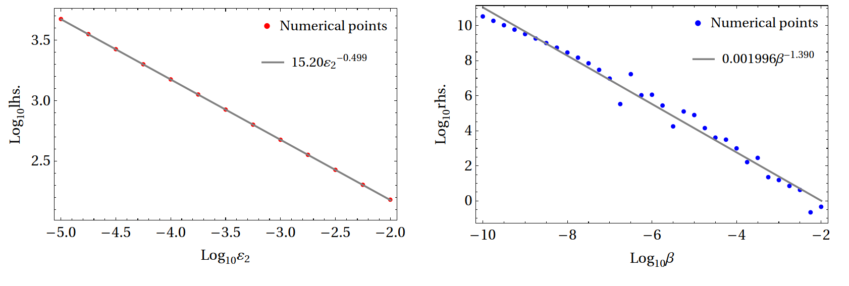
Figure 11: Left panel: numerical results and the fits for the left-hand side of Eq. (LABEL:B13) with respect to regularization parameter $\varepsilon$. Right panel: numerical results and the fits for the right-hand side of Eq. (LABEL:B13) with respect to the parameter $\beta$.

By making use of the results in Eq. (60), we can rewrite the Eq. (54) as

$${\rm Func}(\beta) = {\rm Func}_{0}+\beta PV{\rm Func}_{1}+6.4\times 10^{-5}\beta^{0.6}\left(\sqrt{\varepsilon_{2}}{\rm Func}_{2}\right)+\mathcal{O}(2)\leavevmode\nobreak\ ,$$ (61)

where the integral $PV{\rm Func}_{1}$ and $\sqrt{\varepsilon_{2}}{\rm Func}_{2}$ are finite. Here, the subleading order of the expansion is given by ${\rm Func}_{2}$, instead of the temrs $PV\rm Func_{1}$.

Here, we did not suggest that the regularization parameter $\varepsilon_{0}$ and $\varepsilon_{\pi}$ in Sec. III.2.2 are proportional to $\theta_{k}^{2.788}$. We indeed found that Eq. (34) is proportional to $\sqrt{\varepsilon_{*}}^{-1}$ with the numerical integrals. However, the reliable numerical outcome (like the right-hand side of Fig. 11) for $\theta_{k}\rightarrow 0$ or $\theta_{k}\rightarrow\pi$ is difficult to obtain. Hence, we have to posit the ansatz $\sqrt{\varepsilon_{0}}=\kappa_{0}\theta_{k}^{\nu}$ and $\sqrt{\varepsilon_{\pi}}=\kappa_{\pi}(\pi-\theta_{k})^{\nu}$ with the undetermined parameters $\kappa_{*}$ and $\nu$.

Appendix C Explicit expressions of $\mathbb{P}^{\lambda_{0}\lambda_{1}\lambda_{2}}$

The $\mathbb{P}^{\lambda_{0}\lambda_{1}\lambda_{2}}$ for $\lambda_{*}=\times,+$ used in Sec. III is presented as follows,

$$\mathbb{P}^{\times\times\times} = \frac{1}{\sqrt{2}k_{1}^{2}k_{2}^{2}(k_{1}^{2}+2k_{1}k_{2}\cos\theta_{k}+k_{2}^{2})^{3/2}}\Big{(}-4p^{5}\sin^{4}\theta\sin^{3}\phi\cos\phi(\sin\theta\cos\phi(k_{1}\cos\theta_{k}+k_{2})$$ (62)

$$-k_{1}\cos\theta\sin\theta_{k})(\sin\theta_{k}(k_{2}-p\cos\theta)+p\sin\theta\cos\theta_{k}\cos\phi)\leavevmode\nobreak\ ,$$

$$\mathbb{P}^{\times\times+} = \frac{1}{\sqrt{2}k_{1}^{2}k_{2}^{2}(k_{1}^{2}+2k_{1}k_{2}\cos\theta_{k}+k_{2}^{2})^{3/2}}\Big{(}-2p^{5}\sin^{4}\theta\sin^{2}\phi\cos(2\phi)(\sin\theta\cos\phi(k_{1}\cos\theta_{k}+k_{2})$$ (63)

$$-k_{1}\cos\theta\sin\theta_{k})(\sin\theta_{k}(k_{2}-p\cos\theta)+p\sin\theta\cos\theta_{k}\cos\phi)\leavevmode\nobreak\ ,$$

$$\mathbb{P}^{\times+\times} = \frac{1}{\sqrt{2}k_{1}^{2}k_{2}^{2}(k_{1}^{2}+2k_{1}k_{2}\cos\theta_{k}+k_{2}^{2})^{3/2}}\Big{(}-2p^{4}\sin^{3}\theta\sin^{2}\phi\cos\phi(\sin\theta\cos\phi(k_{1}\cos\theta_{k}+k_{2})$$ (64)

$$-k_{1}\cos\theta\sin\theta_{k})(\cos^{2}\theta_{k}(p^{2}\sin^{2}\theta\cos^{2}\phi-k_{2}^{2})+k_{2}^{2}-2p\cos\theta(-k_{2}\cos^{2}\theta_{k}+k_{2}$$

$$+p\sin\theta\sin\theta_{k}\cos\theta_{k}\cos\phi)+k_{2}p\sin\theta\sin(2\theta_{k})\cos\phi$$

$$+p^{2}\cos^{2}\theta\sin^{2}\theta_{k}-p^{2}\sin^{2}\theta\sin^{2}\phi)\leavevmode\nobreak\ ,$$

$$\mathbb{P}^{\times++} = \frac{1}{\sqrt{2}k_{1}^{2}k_{2}^{2}(k_{1}^{2}+2k_{1}k_{2}\cos\theta_{k}+k_{2}^{2})^{3/2}}\Big{(}-p^{4}\sin^{3}\theta\sin\phi\cos(2\phi)(\sin\theta\cos\phi(k_{1}\cos\theta_{k}+k_{2})$$ (65)

$$-k_{1}\cos\theta\sin\theta_{k})(\cos^{2}\theta_{k}(p^{2}\sin^{2}\theta\cos^{2}\phi-k_{2}^{2})+k_{2}^{2}-2p\cos\theta(-k_{2}\cos^{2}\theta_{k}+k_{2}$$

$$+p\sin\theta\sin\theta_{k}\cos\theta_{k}\cos\phi)+k_{2}p\sin\theta\sin(2\theta_{k})\cos\phi+p^{2}\cos^{2}\theta\sin^{2}\theta_{k}$$

$$-p^{2}\sin^{2}\theta\sin^{2}\phi)\Big{)}\leavevmode\nobreak\ ,$$

$$\mathbb{P}^{+\times\times} = \frac{1}{2\sqrt{2}k_{1}^{2}k_{2}^{2}\left(k_{1}^{2}+2k_{1}k_{2}\cos\theta_{k}+k_{2}^{2}\right)^{3}}\Big{(}-4p^{5}\sin^{3}\theta\sin^{2}\phi\cos\phi(-\sin^{2}\theta\cos^{2}\phi(k_{1}\cos\theta_{k}$$ (66)

$$+k_{2})^{2}(k_{1}^{2}+2k_{1}k_{2}\cos\theta_{k}+k_{2}^{2})+\sin^{2}\theta\sin^{2}\phi(k_{1}^{2}+2k_{1}k_{2}\cos\theta_{k}+k_{2}^{2})^{2}$$

$$+k_{1}^{2}\sin\theta\cos\theta\sin(2\theta_{k})(k_{1}^{2}+3k_{2}^{2})\cos\phi+k_{1}k_{2}\sin(2\theta)\sin\theta_{k}\cos\phi(k_{1}^{2}\cos(2\theta_{k})$$

$$+2k_{1}^{2}+k_{2}^{2})-k_{1}^{2}\cos^{2}\theta\sin^{2}\theta_{k}(k_{1}^{2}+2k_{1}k_{2}\cos\theta_{k}+k_{2}^{2}))(\sin\theta_{k}(k_{2}-p\cos\theta)$$

$$+p\sin\theta\cos\theta_{k}\cos\phi)\leavevmode\nobreak\ ,$$

$$\mathbb{P}^{+\times+} = \frac{1}{2\sqrt{2}k_{1}^{2}k_{2}^{2}\left(k_{1}^{2}+2k_{1}k_{2}\cos\theta_{k}+k_{2}^{2}\right)^{3}}\Big{(}-2p^{5}\sin^{3}\theta\sin\phi\cos(2\phi)(-\sin^{2}\theta\cos^{2}\phi(k_{1}\cos\theta_{k}$$ (67)

$$+k_{2})^{2}(k_{1}^{2}+2k_{1}k_{2}\cos\theta_{k}+k_{2}^{2})+\sin^{2}\theta\sin^{2}\phi(k_{1}^{2}+2k_{1}k_{2}\cos\theta_{k}+k_{2}^{2})^{2}$$

$$+k_{1}^{2}\sin\theta\cos\theta\sin(2\theta_{k})(k_{1}^{2}+3k_{2}^{2})\cos\phi+k_{1}k_{2}\sin(2\theta)\sin\theta_{k}\cos\phi(k_{1}^{2}\cos(2\theta_{k})+2k_{1}^{2}+k_{2}^{2})$$

$$-k_{1}^{2}\cos^{2}\theta\sin^{2}\theta_{k}(k_{1}^{2}+2k_{1}k_{2}\cos\theta_{k}+k_{2}^{2}))(\sin\theta_{k}(k_{2}-p\cos\theta)$$

$$+p\sin\theta\cos\theta_{k}\cos\phi)\Big{)}\leavevmode\nobreak\ ,$$

$$\mathbb{P}^{++\times} = \frac{1}{2\sqrt{2}k_{1}^{2}k_{2}^{2}\left(k_{1}^{2}+2k_{1}k_{2}\cos\theta_{k}+k_{2}^{2}\right)^{3}}\Big{(}2p^{4}\sin^{2}\theta\sin\phi\cos\phi(\sin^{2}\theta\cos^{2}\phi(k_{1}\cos\theta_{k}$$ (68)

$$+k_{2})^{2}(k_{1}^{2}+2k_{1}k_{2}\cos\theta_{k}+k_{2}^{2})+(k_{1}^{2}+2k_{1}k_{2}\cos\theta_{k}+k_{2}^{2})(k_{1}^{2}\cos^{2}\theta\sin^{2}\theta_{k}$$

$$-\sin^{2}\theta\sin^{2}\phi(k_{1}^{2}+2k_{1}k_{2}\cos\theta_{k}+k_{2}^{2}))-k_{1}\sin(2\theta)\sin\theta_{k}\cos\phi(k_{1}\cos\theta_{k}(k_{1}^{2}+3k_{2}^{2})$$

$$+k_{2}(k_{1}^{2}\cos(2\theta_{k})+2k_{1}^{2}+k_{2}^{2})))(\cos^{2}\theta_{k}(p^{2}\sin^{2}\theta\cos^{2}\phi-k_{2}^{2})+k_{2}^{2}$$

$$-2p\cos\theta(k_{2}\sin^{2}\theta_{k}+p\sin\theta\sin\theta_{k}\cos\theta_{k}\cos\phi)+k_{2}p\sin\theta\sin(2\theta_{k})\cos\phi$$

$$+p^{2}\cos^{2}\theta\sin^{2}\theta_{k}-p^{2}\sin^{2}\theta\sin^{2}\phi)\leavevmode\nobreak\ ,$$

$$\mathbb{P}^{+++} = \frac{1}{2\sqrt{2}k_{1}^{2}k_{2}^{2}\left(k_{1}^{2}+2k_{1}k_{2}\cos\theta_{k}+k_{2}^{2}\right)^{3}}\Big{(}p^{4}\sin^{2}\theta\cos(2\phi)(\sin^{2}\theta\cos^{2}\phi(k_{1}\cos\theta_{k}+k_{2})^{2}(k_{1}^{2}$$ (69)

$$+2k_{1}k_{2}\cos\theta_{k}+k_{2}^{2})+(k_{1}^{2}+2k_{1}k_{2}\cos\theta_{k}+k_{2}^{2})(k_{1}^{2}\cos^{2}\theta\sin^{2}\theta_{k}-\sin^{2}\theta\sin^{2}\phi(k_{1}^{2}$$

$$+2k_{1}k_{2}\cos\theta_{k}+k_{2}^{2}))-k_{1}\sin(2\theta)\sin\theta_{k}\cos\phi(k_{1}\cos\theta_{k}(k_{1}^{2}+3k_{2}^{2})+k_{2}(k_{1}^{2}\cos(2\theta_{k})$$

$$+2k_{1}^{2}+k_{2}^{2})))(\cos^{2}\theta_{k}(p^{2}\sin^{2}\theta\cos^{2}\phi-k_{2}^{2})+k_{2}^{2}-2p\cos\theta(k_{2}\sin^{2}\theta_{k}$$

$$+p\sin\theta\sin\theta_{k}\cos\theta_{k}\cos\phi)+k_{2}p\sin\theta\sin(2\theta_{k})\cos\phi+p^{2}\cos^{2}\theta\sin^{2}\theta_{k}$$

$$-p^{2}\sin^{2}\theta\sin^{2}\phi)\Big{)}\leavevmode\nobreak\ .$$

Appendix D SIGWs induced by a peaked curvature power spectrum

Utilizing the variable substitution that can transform the momentum p into three dimensionless quantities $u,v,w$, namely,

$$v=\frac{p}{k_{2}},\hskip 7.11317ptu=\frac{\left|\textbf{k}_{2}-\textbf{p}\right|}{k_{2}},\hskip 7.11317ptw=\frac{\left|\textbf{k}_{1}+\textbf{k}_{2}-\textbf{p}\right|}{k_{2}}.$$

we can evaluate the bispectrum in Eq. (28) as

$$B_{\ast}^{\lambda_{0}\lambda_{1}\lambda_{2}}\left(\textbf{k}_{1},\textbf{k}_{2}\right) = \frac{1}{(2\pi)^{3}\left|\textbf{k}_{1}+\textbf{k}_{2}\right|\left|\textbf{k}_{1}\right|\left|\textbf{k}_{2}\right|\eta^{3}}\int_{0}^{\infty}\int_{|1-v|}^{1+v}\int_{w_{-}}^{w_{+}}\mathcal{D}(v,u,k_{1},k_{2},\theta_{k}){\rm d}v{\rm d}u{\rm d}w$$ (70)

$$\left\{P_{\Phi}(k_{2}u)P_{\Phi}(k_{2}w)P_{\Phi}(k_{2}v)I_{\ast}\left(k_{1},k_{2},\left|\textbf{k}_{1}+\textbf{k}_{2}\right|,v,u,w\right)\mathbb{P}^{\lambda_{0}\lambda_{1}\lambda_{3}}|_{u,w,v}\right\}\leavevmode\nobreak\ ,$$

where $*=0,\pm$, the $I_{*}\left(k_{1},k_{2},\left|\textbf{k}_{1}+\textbf{k}_{2}\right|,v,u,w\right)$ is given in Eq. (29), and

$$\mathcal{D}(v,u,w,k_{1},k_{2},\theta_{k}) = 4uvwk_{2}^{5}\Big{(}-k_{1}^{4}-2(1+u^{2}-v^{2})\cos\theta_{k}k_{1}^{3}k_{2}$$ (71)

$$-\left(u^{4}+(1-v^{2})^{2}-2w^{2}-2u^{2}\left(v^{2}-2\cos^{2}\theta_{k}\right)\right)k_{1}^{2}k_{2}^{2}$$

$$-2(1+u^{2}-v^{2})(u-w)(u+w)\cos\theta_{k}k_{1}k_{2}^{3}+(u^{2}-w^{2})^{2}k_{2}^{4}\Big{)}^{-\frac{1}{2}}\leavevmode\nobreak\ ,$$

$$w_{\pm}(v,u,k_{1},k_{2},\theta_{k}) = \bigg{(}u^{2}+\left(\frac{k_{1}}{k_{2}}\right)^{2}+\frac{k_{1}}{k_{2}}\Big{(}\cos\theta_{k}(1+u^{2}-v^{2})$$ (72)

$$\pm\sin\theta_{k}\sqrt{(-(-1+u^{2})^{2}+2(1+u^{2})v^{2}-v^{4})}\Big{)}\bigg{)}^{\frac{1}{2}}\leavevmode\nobreak\ .$$

Considering a peaked curvature power spectrum $\mathcal{P}_{\Psi}=Ak_{*}\delta(k-k_{*})$, we obtain

$$B_{\star}^{\lambda_{0}\lambda_{1}\lambda_{2}}\left(\textbf{k}_{1},\textbf{k}_{2}\right) = \frac{A^{3}\pi^{3}}{k_{\ast}^{6}\left|\textbf{k}_{1}+\textbf{k}_{2}\right|k_{1}k_{2}^{4}\eta^{3}}\mathcal{D}\left(\frac{k_{\ast}}{k_{2}},\frac{k_{\ast}}{k_{2}},\frac{k_{\ast}}{k_{2}},k_{1},k_{2},\theta_{k}\right)\Theta\left(2\min\left[1,\frac{k_{2}\sin\theta_{k}}{\left|\textbf{k}_{1}+\textbf{k}_{2}\right|}\right]-\frac{k_{2}}{k_{\ast}}\right)$$ (73)

$$\times I_{\star}\left(k_{1},k_{2},\left|\textbf{k}_{1}+\textbf{k}_{2}\right|,\frac{k_{\ast}}{k_{2}},\frac{k_{\ast}}{k_{2}},\frac{k_{\ast}}{k_{2}}\right)\mathbb{P}^{\lambda_{0}\lambda_{1}\lambda_{3}}|_{u=w=v=k_{\ast}/k_{2}}\leavevmode\nobreak\ .$$

where $\star=0,\pm$ and $\Theta(x)$ is Heaviside step functions.

Associating the condition of the flattened non-Gaussianity presented in Tab. 1 with the Heaviside step functions in Eq. (73), it is found that the bispectrum shows to be non-vanishing for small $k_{1},k_{2}\lesssim\mathcal{\mathcal{O}(\sqrt{\epsilon/\eta})}$. It might suggest that the GW detectors on the current frequency band can not detect the bispectrum for the SGIWs induced by the $\delta$-peaked curvature power spectrum.