Riemannian Preconditioned LoRA for Fine-Tuning Foundation Models

Abstract

In this work we study the enhancement of Low Rank Adaptation (LoRA) fine-tuning procedure by introducing a Riemannian preconditioner in its optimization step. Specifically, we introduce an $r\times r$ preconditioner in each gradient step where $r$ is the LoRA rank. This preconditioner requires a small change to existing optimizer code and creates virtually minuscule storage and runtime overhead. Our experimental results with both large language models and text-to-image diffusion models show that with our preconditioner, the convergence and reliability of SGD and AdamW can be significantly enhanced. Moreover, the training process becomes much more robust to hyperparameter choices such as learning rate. Theoretically, we show that fine-tuning a two-layer ReLU network in the convex paramaterization with our preconditioner has convergence rate independent of condition number of the data matrix. This new Riemannian preconditioner, previously explored in classic low-rank matrix recovery, is introduced to deep learning tasks for the first time in our work. We release our code at https://github.com/pilancilab/Riemannian_Preconditioned_LoRA.

1 Introduction

With the expanding scale of neural network models in both vision and language domains, training a neural network from scratch to match the performance of existing large models has become almost unfeasible. As a result, fine-tuning has emerged as a prevalent approach for downstream tasks. Traditional full parameter fine-tuning demands extensive storage, making it impractical for many applications. In contrast, recent advances in Parameter-Efficient Fine-Tuning (PEFT) methods offer a more storage-efficient solution while still delivering strong performance in downstream tasks. A widely-used PEFT method is Low Rank Adaptation, also known as LoRA (Hu et al., 2021), which proposes to add low-rank matrices to existing model weights and only train these additive components. Simply speaking, for a pretrained model weight matrix $W$ of dimension $m$ by $n$, LoRA replaces $W$ with $W+AB^{T}$ where $A,B$ are trainable weight matrices of dimension $m$ by $r$ and $n$ by $r$ for some small rank $r$. In the fine-tuning procedure, $W$ is frozen and we are only optimizing over $A$’s and $B$’s. Compared to full fine-tuning, LoRA introduces fewer trainable parameters. Effectiveness of LoRA has been empirically verified in different fields. Here we note that optimizing LoRA parameters falls into optimizing over low-rank matrices which form a quotient manifold. This motivates the idea of accelerating LoRA training via tools from the field of Riemannian optimization.

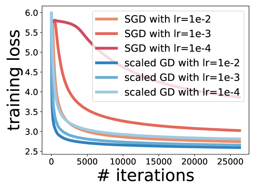
Figure 1: Training loss for fine-tuning a GPT-2 model on E2E NLG challenge with SGD and our method (scaled GD). Our method converges faster than SGD for various learning rates. See Section 4.2 for experimental details.

A line of recent work in low-rank matrix optimization focused on the scaled GD method for conventional low-rank matrix optimization problems involving matrix sensing and robust PCA (Candes et al., 2009). These works consider the following update rule in iteration $t$:

$$A_{t+1}=A_{t}-\alpha(\nabla_{A_{t}}f)(B_{t}^{T}B_{t})^{-1}$$

$$B_{t+1}=B_{t}-\alpha(\nabla_{B_{t}}f)(A_{t}^{T}A_{t})^{-1}$$

where $f$ is the objective function. Scaled GD method suggests scaling by $(A_{t}^{T}A_{t})^{-1}$ to precondition the gradient of $f$ with respect to $B$ and vice versa. This method can be derived from a novel Riemannian metric which takes into consideration both the objective function and constraints (Mishra et al., 2012). Recent work from (Tong et al., 2021b, a) has shown that the above method has better convergence guarantees compared to plain SGD method for various conventional optimization problems, see Section 2 for a detailed discussion. Note the preconditioners in scaled GD are only of dimension $r$ by $r$ thus the storage overhead is negligible for small $r$. Also, unlike most second-order preconditioners such as Hessian inverse, inverting an $r$ by $r$ matrix when $r$ is small introduces ignorable runtime overhead and usually runs as quick as unpreconditioned optimizers. Empirically, small values such as $r=4$ are usually used as default for LoRA fine-tuning, see Figure 3 for runtime comparison for fine-tuning a GPT-2 model with both scaled and unscaled optimizers.

Figure 2: Generation results for prompt “a blue $\langle TOK\rangle$” after fine-tuning on $6$ red vase images of the Stable Diffusion V1.5 model. We vary text-encoder learning rates with U-Net learning rate fixed to default value $1e-4.$ No black images are observed for our method (scaled AdamW)’s generation and AdamW generates only black images for large learning rates. Our method generates photos better capturing the prompt and is more robust to learning rate changes. See Section 4.3.1 for experimental details. The first five photos are presented here.

In this work, we study the application of scaled GD type updates to LoRA fine-tuning. Theoretically, we show convergence guarantees for fine-tuning a reparameterized two-layer ReLU network which is equivalent to ReLU network via convexification. Empirically, we apply this method for LoRA fine-tuning for both large language models and diffusion models. The experimental results show that convergence of both SGD and AdamW is largely enhanced with gradient scaling . Despite accelerated convergence, the optimization procedure becomes much more robust to learning rate changes with this new preconditioner. Figure 1 shows the training loss and Table 1 shows the final scores of different optimizers for fine-tuning a GPT-2 model of medium size on the E2E NLG challenge (Puzikov & Gurevych, 2018). Scaled optimizers significantly improve the performance of unscaled optimizers, see Section 4 for experimental details. To our best knowledge, this is the first work to apply Riemannian optimization knowledge in designing preconditioners for fine-tuning large foundation models, which appears natural considering the matrix factorization feature of LoRA model.

We first give some intuition on our method below, then we include an overview of basic Riemannian optimization concepts as well as related prior works in Section 2. We outline the optimization algorithms with this new introduced preconditioner in Section 3 and present our experimental results in Section 4. We state our convergence theoretic result for related problem in Section 5. Limitations and future work are discussed in Section 6.

1.1 Method Intuition

Consider in the $t$-th iteration pretrained model weight $W$ and its additive low-rank component $A_{t}{B_{t}}^{T}$. Let $X_{t}=W+A_{t}{B_{t}}^{T}$ denote the whole weight matrix and let $\mathcal{L}$ denote the loss function, i.e., $\mathcal{L}(A,B):=\mathcal{L}(W+AB^{T})$. For plain gradient descent method, when step size $\eta$ is small, the updated weight is approximately given by

$$X_{t+1} =W+A_{t+1}B_{t+1}^{T}$$

$$=W+(A_{t}-\eta\nabla_{A_{t}}\mathcal{L})(B_{t}-\eta\nabla_{B_{t}}\mathcal{L})^{T}$$

$$\approx W+A_{t}B_{t}^{T}-\eta A_{t}(\nabla_{B_{t}}\mathcal{L})^{T}-\eta\nabla_{A_{t}}\mathcal{L}B_{t}^{T}$$

$$=X_{t}-\eta A_{t}A_{t}^{T}\nabla_{X_{t}}\mathcal{L}-\eta(\nabla_{X_{t}}\mathcal{L})B_{t}B_{t}^{T},$$

where we ignore the second-order term in the third line. The derivation from the third line to the fourth line comes from the simple fact $(\nabla_{B_{t}}\mathcal{L})^{T}=A_{t}^{T}(\nabla_{X_{t}}\mathcal{L})$ and $\nabla_{A_{t}}\mathcal{L}=(\nabla_{X_{t}}\mathcal{L})B_{t}$. Thus the LoRA update in gradient descent step is approximately constrained to the column space of $A_{t}$ and the row space of $B_{t}$. If we scale $\nabla_{B_{t}}\mathcal{L}$ right by $(A_{t}^{T}A_{t})^{-1}$ and scale $\nabla_{A_{t}}\mathcal{L}$ right by $(B_{t}^{T}B_{t})^{-1}$, which is exactly the preconditioner introduced in Section 1, the scaled update becomes

$$\tilde{X}_{t+1} \approx X_{t}-\eta A_{t}(A_{t}^{T}A_{t})^{-1}A_{t}^{T}(\nabla_{X_{t}}\mathcal{L})$$

$$\qquad~{}~{}-\eta(\nabla_{X_{t}}\mathcal{L})B_{t}(B_{t}^{T}B_{t})^{-1}B_{t}^{T}$$

$$=X_{t}-\eta\mathrm{Proj}_{\text{col}(A_{t})}(\nabla_{X_{t}}\mathcal{L})-\eta\mathrm{Proj}_{\text{row}(B_{t})}(\nabla_{X_{t}}\mathcal{L})^{T}$$

where the update is done according to projection of whole matrix gradient onto column space of $A_{t}$ and row space of $B_{t}$, which better mimics full fine-tuning compared to the unscaled gradient descent step.

2 Prior Work

Our work is closely related to low-rank matrix optimization and we briefly review some basic knowledge and related work in Section 2.1. We intend to apply the introduced preconditioner for accelerating LoRA fine-tuning procedure, which falls into designing preconditioner for PEFT models, and related prior work there is discussed in Section 2.2 and Section 2.3.

2.1 Riemannian Optimization

2.1.1 Inception of a new metric

Optimization over matrix with rank constraint is a common example for optimization over Riemannian submanifolds. Specifically, matrices with fixed rank form a quotient manifold of general matrix field. Let $\mathcal{M}$ denote any Riemannian submanifold, then Riemannian gradient descent usually takes form

$$X_{t+1}=\mathcal{R}(X_{t}-\eta\nabla_{M_{r}}f(X_{t})),$$

where $\mathcal{R}$ is a retraction operator that maps to $\mathcal{M}$. Here, $f$ is the objective function and $\nabla_{M_{r}}f(X_{t})$ denotes Riemannian gradient defined by

$$Df(x)[\eta_{x}]=g_{x}(\nabla_{M_{r}}f(x),\eta_{x})\text{ for all }\eta_{x}\in T_{x}\mathcal{M},$$

where $Df(x)[\eta_{x}]$ is the conventional Euclidean directional derivative of $f$ in the direction $\eta_{x}$. In this definition, $g_{x}$ is a Riemannian metric which maps two elements in the tangent space $T_{x}\mathcal{M}$ to a real number. Note the Riemannian gradient descent method requires the Riemannian gradient $\nabla_{M_{r}}f(X_{t})$ which depends on the choice of the Riemannian metric $g_{x}$.

When it comes to a quotient space $\mathcal{M}/\sim$ where each element $[x]=\{y\in\mathcal{M}:y\sim x\}$ represents an equivalence class, for low-rank matrix problems, each $(A,B)$ pair is equivalent to $(AO,BO^{-1})$ for any $O\in GL(r)$, where $GL(r)$ stands for the general linear group over $r\times r$ invertible matrices, in the sense that they obtain the same objective value. Tangent space $T_{[x]}\mathcal{M}$ respects the equivalence relation $\sim$ by the introduction of horizontal and vertical spaces at each element, i.e., we decompose $T_{x}\mathcal{M}=\mathcal{V}_{x}\oplus\mathcal{H}_{x}$ where $\mathcal{V}_{x}$ is the tangent space of the equivalence class $[x]$ and $\mathcal{H}_{x}$ is its complement. Then each $\eta_{[x]}\in T_{[x]}\mathcal{M}$ corresponds to a unique element in $\mathcal{H}_{x}$ which is called the horizontal lift of $x.$ A Riemannian metric for $\mathcal{M}/\sim$ satisfies

$$g_{[x]}(\eta_{[x]},\xi_{[x]})=g_{x}(\eta_{x},\xi_{x}),$$

where $\eta_{x}$ and $\xi_{x}$ are horizontal lifts of $\eta_{[x]}$ and $\xi_{[x]}$ at $x$. Thus a Riemannian metric on quotient space is invariant along equivalence classes of the quotient space. In (Mishra et al., 2012), the authors describe a new Riemannian metric that draws motivation from regularized Lagrangian and involves both objectives and constraints. When specialized to least squares matrix decomposition problem of form $\|AB^{T}-Y\|_{F}^{2}/2$, following derivation (33) in (Mishra & Sepulchre, 2016), we get the following metric on quotient space $[x]=(A,B)$,

$$g_{[x]}(\xi_{[x]},\eta_{[x]})=\langle\xi_{A},\eta_{A}B^{T}B\rangle+\langle\xi_{B},\eta_{B}A^{T}A\rangle.$$ (1)

Under this new metric, the Riemannian gradient descent takes step as

$$\frac{\partial}{\partial A}\rightarrow(\frac{\partial}{\partial A})(B^{T}B)^{-1},\frac{\partial}{\partial B}\rightarrow(\frac{\partial}{\partial B})(A^{T}A)^{-1}.$$ (2)

For details in the design of the new metric (1) and its connection with sequential quadratic programming (SQP), we point readers to (Mishra & Sepulchre, 2016) and (Mishra et al., 2012) which include a thorough explanation and visualization on Riemannian optimization concepts.

2.1.2 Improved convergence guarantees

Several recent studies have made theoretic contributions to the convergence rate of scaled GD method which employs the preconditioner (2). Specifically, in (Tong et al., 2021a, b), the authors show local convergence of scaled GD method with better convergence rate independent of data condition number compared to plain gradient descent method for some classic low-rank matrix optimization problem including matrix sensing, robust PCA, etc. The authors of (Jia et al., 2023) show global convergence of scaled GD method with rate independent of data condition number for least squares matrix decomposition problem $\|AB^{T}-Y\|_{F}^{2}/2$.

2.1.3 Additional variants

Different variants of scaled GD have been proposed and studied. In (Zhang et al., 2023c), the authors suggest to use $(A^{T}A+\lambda I)^{-1}$ and $(B^{T}B+\lambda I)^{-1}$ with some fixed $\lambda>0$ in place of (2) for tackling overparametrization and ill-conditioness in matrix sensing problems. In (Zhang et al., 2023b), the authors suggest using $(A^{T}A+\lambda_{t}I)^{-1}$ where $\lambda_{t+1}=\beta\lambda_{t}$ (similar change for $B$), i.e., using an exponentially decay regularization term. (Zhang et al., 2023c) proposes precGD method which sets $\lambda_{t}=\sqrt{f(A_{t}B_{t}^{T})}$. (Tong et al., 2022; Ma et al., 2023) present extension of scaled GD method to tensor optimization problem. (Jia et al., 2023) analyzes AltScaledGD method which updates $A$ and $B$ alternatively and shows that such method has better convergence rate for larger step size.

2.2 Preconditioners in Deep Learning

Current deep learning training is dominated by gradient-based method which follows a descent direction to update parameters for decreasing objective value. For accelerating such training procedure, more advanced techniques such as Adagrad (Duchi et al., 2011) proposes to scale gradient based on their variance. Specifically, $G_{t}^{-1/2}$ is used as gradient preconditioner where $G_{t}$ is accumulated outer product of historic subgradients. More practical optimizers such as Adam (Kingma & Ba, 2017) and AdamW (Loshchilov & Hutter, 2019) perform like a diagonal version of Adagrad and are the main training tools for most deep learning models in various fields. More recently, Shampoo (Gupta et al., 2018) has been proposed which uses a left preconditioner and a right preconditioner for a weight matrix. Shampoo is in spirit close to Adagrad but requires much less storage.

In contrast with the preconditioners designed for accelerating optimization procedure for general deep learning models. We study a specific preconditioner designed for LoRA fine-tuning model which exploits its low rank matrix factorization property and borrows from Riemannian optimization knowledge.

2.3 PEFT Fine-Tuning Review

Current commonly-used deep learning models are growing larger and larger, making full fine-tuning for downstream tasks nearly impossible. A line of parameter-efficient fine-tuning methods emerges and has been used in various fields. These methods aim at achieving low fine-tuning loss with fewer trainable parameters. One popular PEFT method is LoRA (Hu et al., 2021), which proposes to add a low-rank adaptation to each existing weight matrix. By factorizing the update into two low-rank matrices, LoRA is able to achieve similar fine-tuning result as full fine-tuning with 10,000 times fewer parameters. LoRA has shown good performance in both language model fine-tuning and vision model fine-tuning. Variants of LoRA method involve DyLoRA (Valipour et al., 2023), IncreLoRA (Zhang et al., 2023a), and AdaLoRA (Zhang et al., 2023d), all focus on dynamically adjusting the rank hyperparameter. GLoRA (Chavan et al., 2023) generalizes LoRA by introducing a prompt module; Delta-LoRA (Zi et al., 2023) proposes to simultaneously update pretrained model weights by difference of LoRA weights. QLoRA (Dettmers et al., 2023) exploits quantized LoRA model which further reduces the model size. Besides such additive methods, there are also multiplicative PEFT methods such as the orthogonal fine-tuning method (OFT) (Qiu et al., 2023) and its variant BOFT (Liu et al., 2023).

Though LoRA has become very popular and different variants emerge, current LoRA training mainly exploits AdamW optimizer and we are unaware of any prior work studying acceleration of LoRA training given its special low-rank matrix factorization nature. Our work shows that by regrouping trainable parameters and apply an $r\times r$ preconditioner, the optimization procedure of LoRA can be significantly enhanced with negligible storage and runtime overhead.

3 Methodology

In this section, we describe formally the optimization algorithms we use for accelerating LoRA training. Let $\mathcal{L}$ denote the loss function and $(A^{(t)},B^{(t)})$ denote the pair of LoRA parameters in the $t$-th iteration. To apply gradient scaling to SGD method, we follow exactly what has been discussed in previous sections and use $(B^{(t-1)^{T}}B^{(t-1)}+\delta I)^{-1}$ to scale gradient $\nabla_{A^{(t-1)}}\mathcal{L}$ and vice versa. Note here a small $\delta$ is used to tackle the case when either $B^{(t-1)^{T}}B^{(t-1)}$ or $A^{(t-1)^{T}}A^{(t-1)}$ is not invertible. Empirically, we take $\delta=1e-6$. For sake of page limit, see Appendix B for the complete algorithm.

The conventional scaled GD methods studied for classic low-rank matrix optimization problems are only based on the gradient method. We note that when fine-tuning deep learning models, AdamW is more popular than SGD due to its stability and fast convergence. However, when both methods behave similarly, SGD is actually advantageous since it has smaller storage overhead compared to AdamW. In later sections, we show that scaled GD empirically closes the gap between SGD and AdamW. To extend gradient scaling method to AdamW, one could apply the preconditioner at the gradient computation step, i.e., “scaling step” in Algorithm 1. A reasonable alternative is to apply the scaling to the averaged gradient, i.e., “final step” in Algorithm 1. Empirically, we find that scaling the gradient in each single iteration behaves much better than scaling the averaged gradient at the final step, thus we scale each single gradient in AdamW algorithm and name it scaled AdamW method. For clarity, Algorithm 1 only outlines the update rule for $A^{(t)}$. Update for $B^{(t)}$ can be derived similarly.

Algorithm 1 Scaled AdamW method for LoRA fine-tuning

  AdamW input: learning rate $\eta$, weight decay $\lambda$, $\beta_{1},\beta_{2},\epsilon$.

  LoRA initialization: starting point $A=A^{(0)},B=B^{(0)}.$

  Scaled AdamW update: for $t=1,2,...,T$ do

$$A^{(t)}=A^{(t-1)}-\eta\lambda A^{(t-1)}$$

$$g_{A}^{(t)}=\nabla_{A^{(t-1)}}\mathcal{L}(B^{(t-1)^{T}}B^{(t-1)}+\delta I)^{-1}$$

$\qquad\qquad\qquad\qquad\qquad\qquad\qquad\qquad\rightarrow\textbf{scaling step}$

$$m_{A}^{(t)}=\beta_{1}m_{A}^{(t-1)}+(1-\beta_{1})g_{A}^{(t)}$$

$$v_{A}^{(t)}=\beta_{2}v_{A}^{(t-1)}+(1-\beta_{2}){g_{A}^{(t)}}^{2}$$

$$\widehat{m_{A}^{(t)}}=m_{A}^{(t)}/(1-\beta_{1}^{t})$$

$$\widehat{v}_{A}^{(t)}=v_{A}^{(t)}/(1-\beta_{2}^{t})$$

$\qquad\quad A^{(t)}=A^{(t)}-\eta\widehat{m_{A}^{(t)}}/(\sqrt{\widehat{v}_{A}^{(t)}}+\epsilon)~{}\rightarrow~{}\textbf{final step}$

4 Experiments

We exploit using the new Riemannian preconditioner for accelerating LoRA training in different deep learning models including language models and vision models. For language models, we first show that this new preconditioner improves traditional optimizers for GPT-2 model fine-tuning which is used for experiments in original LoRA project (Hu et al., 2021). Empirical results show that scaled optimizers uniformly improve the performance of unscaled optimizers for varying LoRA ranks, datasets, and model sizes on all evaluation metrics. We then proceed to tune a much newer LLM model named Mistral 7B (Jiang et al., 2023) which has recently been shown to outperform Llama 2 13B on various benchmarks while having much fewer parameters. Our empirical result shows that scaled optimizers significantly improve the unscaled optimizers by a large margin for fine-tuning this new model with LoRA. See Section 4.2 for our language model experimental results. We also explore applying the new preconditioner for LoRA fine-tuning for diffusion models. In Section 4.3, we first show its effectiveness for tuning a commonly used stable diffusion model on object generation and we then move on to show its superiority for tuning the Mix-of-Show variant which we find better for high-quality face generation. We observe that with this new preconditioner added to the optimization procedure, the training becomes much more robust to learning rate changes, which has significant practical benefit since learning rate tuning is more sensitive in diffusion model and learning rate which is a bit off may generate totally nonsense images. This can be directly observed from Figure 2. Moreover, it’s quite challenging to come up with metrics that correlate with artistic quality. Monitoring training loss usually fails to capture the generation quality due to the denoising nature of diffusion model. Thus a more reliable optimizer is needed.

4.1 Runtime Comparison

Figure 3: Runtime for LoRA fine-tuning GPT-2 medium model with different optimizers. Our scaled methods introduce negligible runtime overhead and train as fast as unscaled methods. See Section 4.1 for experimental details.

A common stereotype about preconditioning is its cumbersomeness and heavy computation complexity. This is likely due to Hessian-inverse type second-order preconditioner usually involves large size preconditioners and complex computation procedures, which is not the case for the preconditioners we consider. In each iteration, we use current value of $(A^{T}A)^{-1}$ to precondition gradient of $B$. The preconditioner is easily obtained and is of small size, the only overhead is we need the value of parameter $A$ when optimizing parameter $B$. This can be easily done by grouping the LoRA parameters during traning given the fact that LoRA parameters are stored in the order $\{A_{1},B_{1},A_{2},B_{2},\dots\}$ in most LoRA libraries. As a warm up, we present a runtime comparison between scaled optimizers and their unscaled counterparts for fine-tuning a GPT-2 medium model on E2E NLG challenge, see Section 4.2.1 for experimental details. Figure 3 shows the runtime used for different optimizers for the fine-tuning task trained on NVIDIA A100 GPUs. Note there is little difference between the scaled optimizers and unscaled ones, which verifies that our preconditioner is indeed very practical.

4.2 LLM Fine-Tuning

In this section, we study the fine-tuning task for GPT-2 model and Mistral 7B model with our new scaled optimizers. Empirically, we observe that our scaled optimizers outperform unscaled optimizers by a large margin for various tasks, datasets, LoRA ranks, model sizes, model types, and benchmarks, which demonstrates the superiority of gradient scaling in training LoRA models. See below and also Appendix C for all our experiments.

4.2.1 GPT-2

We exploit the new preconditioner for LoRA fine-tuning for GPT-2 models. We follow exactly the same experimental setup as (Hu et al., 2021) except that here we tune learning rate individually using grid search for different methods being tested, see Appendix C.1 for experimental details and training hyperparameters. Table 1 shows the final score for fine-tuning GPT-2 medium model with LoRA rank $4$ on E2E natural language generation challenge. It can be observed that scaled GD method closes the gap between SGD and AdamW and behaves comparable to AdamW while demanding less storage. Scaled AdamW method improves score of AdamW method on all evaluation metrics, which reveals that the new preconditioner is advantageous even for gradient computation normalized by gradient variance in AdamW method. This has never been considered in any prior work. See Appendix C.1 for experimental results for different LoRA ranks, different datasets, and different model sizes. Our scaled optimizers gain uniform improvement over unscaled optimizers for all tests.

Method	E2E
	BLEU	NIST	MET	ROUGE-L	CIDEr
SGDr=4	68.7	8.66	45.8	70.4	2.42
scaled GD (ours)r=4	70.5	8.82	46.6	72.1	2.52
AdamWr=4	70.6	8.84	46.9	71.8	2.55
scaled AdamW (ours)r=4	70.8	8.90	46.9	72.5	2.56

Table 1: Scores for LoRA fine-tuning GPT-2 medium model on E2E Natural Language Generation challenge with different optimizers. Our scaled optimizers outperform unscaled optimizers on all evaluation metrics and scaled GD closes the performance gap between SGD and AdamW. See Section 4.2.1 for experimental details.

4.2.2 Mistral 7B

Mistral 7B is a recent language model released by the Mistral AI team (Jiang et al., 2023) which has been shown to outperform Llama 2 13B on all benchmarks and Llama 1 34B on many benchmarks (Mistral AI team, 2023), and thus is considered the most powerful language models for its size to date. We experiment our scaled optimizers with this new language model on the GLUE benchmark (Wang et al., 2018) for natural language understanding problems. We follow common strategy for fine-tuning Mistral 7B model and set learning rate to be $5e-5$ for AdamW-type methods (Labonne, 2024). Empirically, we find SGD-type methods work for much larger learning rate and thus we set learning rate to be $5e-3$ which generates reasonable fine-tuning results. All rest settings are default as in HuggingFace transformers trainer class (Huggingface team, 2023). For quicker training, we use $4$-bit quantized version of Mistral 7B V0.1 as our base model and LoRA factors are injected to each linear layer with rank $r=16.$ We train for $5$ total epochs with batch size $8$. Table 2 shows the final fine-tuning results. Notably that our scaled optimizers outperform unscaled optimizers by a large margin, which demonstrates the effectiveness of gradient scaling for fine-tuning Mistral 7B model. See Appendix C.2 for training hyperparameter selection. All choices are explained there and nothing is particularly tuned in favor of our methods.

Method	GLUE
	MNLI	SST-2	MRPC	CoLA	QNLI	QQP	RTE	STS-B	WNLI	Avg.
SGDr=16	88.15	96.44	66.67	53.84	90.68	88.59	55.96	57.61	47.89	71.76
scaled GD (ours)r=16	90.21	96.56	79.66	67.95	92.60	91.15	83.03	76.74	46.48	80.49
AdamWr=16	89.86	96.79	89.71	68.07	94.58	91.24	78.34	91.52	56.34	84.05
scaled AdamW (ours)r=16	90.68	96.44	90.69	70.56	94.38	92.22	89.17	91.90	63.38	86.60

Table 2: Scores for LoRA fine-tuning 4-bit quantized Mistral 7B model on GLUE benchmark for Natural Language Understanding (NLU) challenges with different optimizers. Our scaled optimizers outperform unscaled optimizers by a large margin on most evaluation metrics. See Section 4.2.2 for experimental details.

4.3 Diffusion Model Fine-Tuning

Diffusion models are now used for various image generation tasks and LoRA has been widely used for fine-tuning diffusion models. Here we start with a commonly used basic Stable Diffusion V1.5 model and show the effectiveness of applying our new preconditioner in LoRA fine-tuning for object image generation. Then we experiment with the Mix-of-Show model (Gu et al., 2023) which we find able to generate high-quality face images among different variants of custom diffusion models. We observe that with gradient scaling, image generation becomes much more robust to learning rate changes, which is a reflection of the fact that our new preconditioner stabilizes model training procedure against learning rate variations. This has large practical benefit since learning rate choice can be core to image generation models where small difference in learning rate can produce images of very different quality and learning rate that is a bit off may produce vague pictures, which can be seen from Figure 2 and 4. Furthermore, it’s widely observed that training loss is useless in monitoring image generation quality when training diffusion models. Thus a better optimizer which is more robust to learning rate choices is very important. See Appendix D for experimental details for diffusion model fine-tuning tasks.

4.3.1 Object generation

We build our object generation experiments on a popular stable diffusion fine-tuning repository (Ryu, 2023) with Stable Diffusion V1.5 as the base model. We follow the default settings there and tune both the U-Net and the text encoder where LoRA parameters are injected. The default optimizer is AdamW. For all experiments, we fix the U-Net fine-tuning learning rate as default value $1e-4$ which we find important for generating recognizable images. After fine-tuning on $6$ images of a red vase with title “a photo of $\langle TOK\rangle$”, Figure 2 shows the generation results for prompt “a blue $\langle TOK\rangle$”. With large learning rate $1e-2$ for text encoder fine-tuning, AdamW produces out-of-distribution results while our method produces satisfactory images. With default learning rate setting , AdamW still fails to capture the prompt information and generates only red vases. Instead, scaled AdamW with default learning rate is able to produce the desired blue vase. Note here we only generate five images for all tests and the result is not cherry-pick. AdamW turns out to be able to generate the desired blue vase for learning rate value such as $1e-6$. See Appendix D.1 for other target object generation including chairs and dogs. Scaled AdamW improves AdamW for all experiments.

4.3.2 Face generation

Face generation is a more challenging task compared to object generation and we thus switch to Mix-of-Show (Gu et al., 2023) variant of custom diffusion model which is originally designed for multi-concept LoRA and has been recognized to be able to generate high-quality face images. For better visualization of differences between different LoRA optimization methods, we turn off embedding fine-tuning and tune only text-encoders and U-Nets where LoRA factors are injected. We follow all default settings in original Mix-of-Show project except for the optimizer component. The default optimizer is AdamW and default learning rate is $1e-5$ for text-encoder fine-tuning and $1e-4$ for U-Net fine-tuning. We use $14$ images of Potter provided in the original project repository where the character name is replaced with $\langle TOK\rangle$ in captions of the training images. Figure 4 shows generation results for prompt “a pencil sketch of $\langle TOK\rangle$” for various step sizes. Our method (scaled AdamW) generates visually better images more resemble a pencil sketch, which demonstrates its effectiveness in generating images of higher quality and also its robustness to learning rate changes. See Appendix D.2.1 for generation results for more prompts and also for Hermoine character with different LoRA parameter fusion coefficients. See also Appendix D.2.2 for generation results including SGD and scaled GD methods for varying learning rates. Our observation persists in all those generation results.

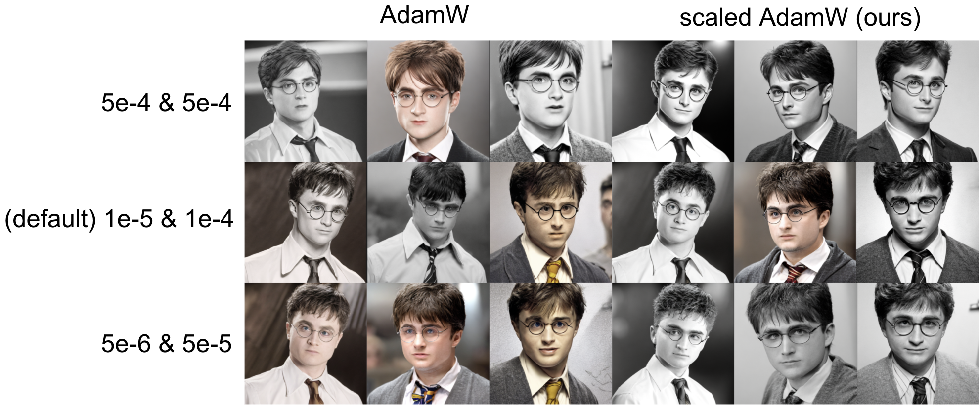
Figure 4: Generation results for prompt “a pencil sketch of $\langle TOK\rangle$” by Mix-of-Show model with different optimizers and various learning rates. Our method (scaled AdamW) generates photos better capturing the prompt, i.e., a pencil sketch, and is more robust to learning rate choices. See Section 4.3.2 for experimental details. The first three photos are presented here.

5 Theory

When scaled GD is applied to deep learning models, nonlinearities in such models usually make theoretic analysis intractable. To tackle this, we instead study an equivalent problem to two-layer ReLU neural network. We first introduce the concept of arrangement matrices. For data matrix $X\in\mathbb{R}^{n\times d}$ and any arbitrary vector $u\in\mathbb{R}^{d}$, We consider the set of diagonal matrices

$$\mathcal{D}:=\{\text{diag}({\mathbbm{1}}\{Xu\geq 0\})\},$$

which takes value $1$ or $0$ along the diagonals that indicate the set of possible arrangement activation patterns for the ReLU activation. Indeed, we can enumerate the set of sign patterns as $\mathcal{D}=\{D_{i}\}_{i=1}^{P}$ where $P$ is bounded by

$$P\leq 2r\left(\frac{e(n-1)}{r}\right)^{r}$$

for $r=\text{rank}(X)$ (Pilanci & Ergen, 2020; Stanley et al., 2004). We note that two-layer ReLU model is equivalent to the problem below for squared loss through convexification under mild conditions (Mishkin et al., 2022)

$$\min_{W_{i}}\frac{1}{2}\|\sum_{i=1}^{P}D_{i}XW_{i}-Y\|_{F}^{2}.$$

Therefore, we base our analysis on fine-tuning the above model and shows that the convergence rate of problem below with scaled GD method (Algorithm 2) has no dependence on condition number of data matrix $X$,

$$\min_{A_{i},B_{i}}\frac{1}{2}\|\sum_{i=1}^{P}D_{i}X(W_{i}+A_{i}B_{i}^{T})-Y\|_{F}^{2},$$ (3)

where $X\in\mathbb{R}^{n\times d},A_{i}\in\mathbb{R}^{d\times r},B_{i}\in\mathbb{R}^{c\times r},Y\in\mathbb{R}^{n\times c}.$ Here we consider $Y=\sum_{i=1}^{P}D_{i}X(W_{i}+A_{\star}^{i}{B_{\star}^{i}}^{T})$. Denote $X_{\star}^{i}=A_{\star}^{i}{B_{\star}^{i}}^{T}=U_{\star}^{i}\Sigma_{\star}^{i}{V_{\star}^{i}}^{T}$ with $U_{\star}^{i}\Sigma_{\star}^{i}{V_{\star}^{i}}^{T}$ being the singular value decomposition of $X_{\star}^{i}$. Denote $F_{\star}^{i}=[A_{\star}^{i},B_{\star}^{i}]^{T}$ and $F_{t}^{i}=[A_{t}^{i},B_{t}^{i}]^{T}$ with $A_{t}^{i}$ and $B_{t}^{i}$ denote the value of $(A_{i},B_{i})$ at $t$-th iteration. Let $\sigma_{r}(\cdot)$ denote the $r$-th largest singular value.

We first introduce the definition of Restricted Isometry Property (RIP) and illustrate the assumptions required for our theorem to hold,

Definition 5.1.

(RIP (Recht et al., 2010)) The matrix $A\in\mathbb{R}^{n\times d}$ satisfies rank-$r$ RIP with a constant $\delta_{r}\in[0,1)$ if for all matrices $M\in\mathbb{R}^{d\times c}$ of rank at most $r$, the below holds,

$$(1-\delta_{r})\|M\|_{F}^{2}\leq\|AM\|_{F}^{2}\leq(1+\delta_{r})\|M\|_{F}^{2}.$$

Assumption 5.2.

Suppose that $D_{i}X$ obeys the $2r$-RIP with a constant $\delta_{2r}^{i}$ for each $i$, and $\|X^{T}{D_{i}}^{T}D_{j}X\|_{2}\leq\min(\frac{\delta_{2r}^{i}\|X_{\star}^{i}\|_{F}}{P\|X_{\star}^{j}\|_{F}},\frac{0.12}{7P(P+1)})$ for any $j\neq i.$

Note for matrix $X$ with i.i.d Gaussian entries $\mathcal{N}(0,1/d\|D_{i}\|_{0})$, $D_{i}X$ satisfies RIP for a constant $\delta$ when $\|D_{i}\|_{0}$ is on the order of $r(d+c)/(d\delta^{2})$. See (Recht et al., 2010) for other measurement ensembles satisfy the RIP property. Note also $\|X^{T}{D_{i}}^{T}D_{j}X\|_{2}\leq\|X^{T}X\|_{2}$ for all $(i,j)$’s. Thus bounding $\|X^{T}{D_{i}}^{T}D_{j}X\|_{2}$ amounts to bounding largest singular value of empirical covariance matrix. We consider a specific initialization strategy here which is an extension of spectral initialization for multiple terms as below,

Definition 5.3.

(Extended Spectral Initialization) Let $A_{0}^{i}{B_{0}^{i}}^{T}$ be the best rank-$r$ approximation of $(D_{i}X)^{T}(Y-\sum_{j=1}^{P}D_{j}XW_{j})$ for each $i.$

Now, we are ready to state our main convergence result as follows,

Theorem 5.4.

Under Assumption 5.2 with $\delta_{2r}^{i}\leq 0.01$ for each $i$. With extended spectral initialization described in Definition 5.3, $\|A_{t}^{i}{B_{t}^{i}}^{T}-X_{\star}^{i}\|_{F}\leq 1.5\text{dist}(F_{t}^{i},F_{\star}^{i})$. In addition, if the step size $0<\eta\leq 2/3$, then the $(t+1)$-th iteration $F_{t+1}^{i}$ satisfies

$$\max_{i}(\text{dist}(F_{t+1}^{i},F_{\star}^{i}))\leq(1-0.5\eta)\max_{i}(\text{dist}(F_{t}^{i},F_{\star}^{i})).$$

Proof.

See Appendix A. ∎

Our result mainly builds on results in (Tong et al., 2021b) and can be viewed as an extension of matrix sensing problem considered there.

6 Conclusion

In this project, we borrow tools from Riemannian optimization to enhance LoRA fine-tuning. Specifically, we study the application of scaled GD method which introduces a new $r\times r$ preconditioner for low-rank matrix optimization problems to LoRA fine-tuning procedure. Prior to our work, theoretic convergence for scaled GD method has been established for classic low-rank matrix optimization problems and we first introduce it to deep learning models considering the low-rank nature of LoRA. We test this new preconditioner for both language model fine-tuning and diffusion model fine-tuning and observe that scaled gradient helps both SGD and AdamW methods while only SGD-type method has been considered in prior work. Moreover, the new preconditioner helps stabilizing the training procedure against step size changes which can be observed from our diffusion model fine-tuning result. Theoretically, we show convergence of fine-tuning a reparametrized two-layer ReLU model, which is an extension of prior convergence result for matrix sensing problems.

There are also several limitations to our work. Firstly, We only tested the plain scaled gradient method, though it already gains large improvement, variants of this method discussed in Section 2 also deserve exploration. Besides, though scaled gradient combined with AdamW method has been empirically observed to be useful, there is still a lack of theoretical justification.

7 Acknowledgements

This work was supported in part by the National Science Foundation (NSF) under Grant DMS-2134248; in part by the NSF CAREER Award under Grant CCF-2236829; in part by the U.S. Army Research Office Early Career Award under Grant W911NF-21-1-0242; in part by the Precourt Institute for Energy and the SystemX Alliance at Stanford University.

Appendix A Proof of Theorem 5.4

Note problem (3) is equivalent to the problem below up to a change of labels,

$$\min_{A_{i},B_{i}}{\|\sum_{i=1}^{P}C_{i}A_{i}B_{i}^{T}-Y\|_{F}^{2}},$$ (4)

where $C_{i}\in\mathbb{R}^{n\times d},A_{i}\in\mathbb{R}^{d\times r},B_{i}\in\mathbb{R}^{c\times r},Y\in\mathbb{R}^{n\times c}.$ Consider $Y=\sum_{i=1}^{P}C_{i}A_{\star}^{i}{B_{\star}^{i}}^{T}$. Denote $X_{\star}^{i}=A_{\star}^{i}{B_{\star}^{i}}^{T}=U_{\star}^{i}\Sigma_{\star}^{i}{V_{\star}^{i}}^{T}$ where $U_{\star}^{i}\Sigma_{\star}^{i}{V_{\star}^{i}}^{T}$ is the singular value decomposition of $X_{\star}^{i}$. Denote $F_{\star}^{i}=[A_{\star}^{i},B_{\star}^{i}]^{T}.$ For any $F=[A,B]^{T}$, consider the following distance metric

$$\text{dist}^{2}(F,F_{\star}^{i})=\inf_{Q\in{\color[rgb]{0,0,0}GL(r)}}\left\|(AQ-A_{\star}^{i}){\Sigma_{\star}^{i}}^{1/2}\right\|_{F}^{2}+\left\|(BQ^{-T}-B_{\star}^{i}){\Sigma_{\star}^{i}}^{1/2}\right\|_{F}^{2},$$ (5)

where $GL(r)$ denotes the set of invertible matrix in $\mathbb{R}^{r\times r}$. Let $\sigma_{r}(\cdot)$ denote the $r$th largest singular value and $\kappa_{i}$ denote condition number of $X_{\star}^{i}$. Consider the following scaled GD step:

$$A_{t+1}^{i}=A_{t}^{i}-\eta C_{i}^{T}(\sum_{j}C_{j}A_{t}^{j}{B_{t}^{j}}^{T}-Y)B_{t}^{i}({B_{t}^{i}}^{T}B_{t}^{i})^{-1},$$

$$B_{t+1}^{i}=B_{t}^{i}-\eta(C_{i}^{T}(\sum_{j}C_{j}A_{t}^{j}{B_{t}^{j}}^{T}-Y))^{T}A_{t}^{i}({A_{t}^{i}}^{T}A_{t}^{i})^{-1}.$$

Before we begin the main proof, we need the following partial Frobenius norm which has been introduced in Section A.3 in (Tong et al., 2021b) with some important properties studied there.

Definition A.1.

(Partial Frobenius norm) For any matrix $X$, its partial Frobenius norm of order $r$ is given by $l_{2}$ norm of vectors composed by its top-$r$ singular values,

$$\|X\|_{F,r}=\sqrt{\sum_{i=1}^{r}\sigma_{i}^{2}(X)}.$$

Now we start the proof by first proving some useful lemmas.

Lemma A.2.

Under Assumption 5.2, let $F_{0}^{i}=[A_{0}^{i},B_{0}^{i}]^{T}$, then the extented spectral initialization in Definition 5.3 satisfies

$$\text{dist}(F_{0}^{i},F_{\star}^{i})\leq 10\delta_{2r}^{i}\sqrt{r}\kappa_{i}\sigma_{r}(X_{\star}^{i}).$$

Proof.

According to Lemma 11 in (Tong et al., 2021b), since $A_{0}^{i}{B_{0}^{i}}^{T}-X_{\star}^{i}$ has rank at most $2r$,

$$\text{dist}(F_{0}^{i},F_{\star}^{i}) \leq\sqrt{\sqrt{2}+1}\|A_{0}^{i}{B_{0}^{i}}^{T}-X_{\star}^{i}\|_{F},$$

$$\leq\sqrt{2(\sqrt{2}+1)}\|A_{0}^{i}{B_{0}^{i}}^{T}-X_{\star}^{i}\|_{{\color[rgb]{0,0,0}F,r}}.$$

Since $A_{0}^{i}{B_{0}^{i}}^{T}$ is the best rank $r$ approximation of $C_{i}^{T}Y=\sum_{j=1}^{P}C_{i}^{T}C_{j}X_{\star}^{j}$. Then

$$\|A_{0}^{i}{B_{0}^{i}}^{T}-X_{\star}^{i}\|_{F,r} \leq\|\sum_{j=1}^{P}C_{i}^{T}C_{j}X_{\star}^{j}-A_{0}^{i}{B_{0}^{i}}^{T}\|_{F,r}+\|\sum_{j=1}^{P}C_{i}^{T}C_{j}X_{\star}^{j}-X_{\star}^{i}\|_{F,r},$$

$$\leq 2\|(C_{i}^{T}C_{i}-I)X_{\star}^{i}+\sum_{j\neq i}C_{i}^{T}C_{j}X_{\star}^{j}\|_{F,r},$$

$$\leq{\color[rgb]{0,0,0}2\delta_{2r}^{i}\|X_{\star}^{i}\|_{F}}+2\sum_{j\neq i}\|C_{i}^{T}C_{j}X_{\star}^{j}\|_{F},$$

where the last inequality follows Lemma 15 and inequality (50) in (Tong et al., 2021b). Therefore,

$$\text{dist}(F_{0}^{i},F_{\star}^{i}) \leq 5\delta_{2r}^{i}\|X_{\star}^{i}\|_{F}+5\sum_{j\neq i}{\color[rgb]{0,0,0}\|C_{i}^{T}C_{j}X_{\star}^{j}\|_{F}},$$

$$\leq 10\delta_{2r}^{i}\|X_{\star}^{i}\|_{F}\leq 10\delta_{2r}^{i}\sqrt{r}\kappa_{i}\sigma_{r}(X_{\star}^{i}).$$

∎

Lemma A.3.

(Contraction) Under assumption 5.2 with $\delta_{2r}^{i}\leq 0.01$. If the $t$-th iterate satisfies $\text{dist}(F_{t}^{i},F_{\star}^{i})\leq 0.1\sigma_{r}(X_{\star}^{i})$ where $F_{t}^{i}=[A_{t}^{i},B_{t}^{i}]^{T}$, then $\|A_{t}^{i}{B_{t}^{i}}^{T}-X_{\star}^{i}\|_{F}\leq 1.5\text{dist}(F_{t}^{i},F_{\star}^{i})$. In addition, if the step size $0<\eta\leq 2/3$, then the $(t+1)$-th iteration $F_{t+1}^{i}$ satisfies

$$\max(\text{dist}(F_{t+1}^{i},F_{\star}^{i}))\leq(1-0.5\eta)\max(\text{dist}(F_{t}^{i},F_{\star}^{i})).$$

Proof.

We first show $\|A_{t}^{i}{B_{t}^{i}}^{T}-X_{\star}^{i}\|_{F}\leq 1.5\text{dist}(F_{t}^{i},F_{\star}^{i}).$ According to Lemma 9 in (Tong et al., 2021b), we know $Q_{t}^{i},$ the optimal alignment matrix between $F_{t}^{i}$ and $F_{\star}^{i}$ , i.e., the optimal value of problem (4) with $F$ replaced by $F_{t}^{i}$ is attained at $Q_{t}^{i}$, exists, denote $A^{i}=A_{t}^{i}Q_{t}^{i},B^{i}=B_{t}^{i}{Q_{t}^{i}}^{-T},\triangle_{A}^{i}=A^{i}-A_{\star}^{i},\triangle_{B}^{i}=B^{i}-B_{\star}^{i}.$ By derivation (45) in (Tong et al., 2021b), we further know for $\epsilon=0.1,$

$$\|\triangle_{A}^{i}{\Sigma_{\star}^{i}}^{-1/2}\|_{2}\lor\|\triangle_{B}^{i}{\Sigma_{\star}^{i}}^{-1/2}\|_{2}\leq\epsilon,$$

where $\lor$ denotes maximum. Note

$$\|A_{t}^{i}{B_{t}^{i}}^{T}-X_{\star}^{i}\|_{F} =\|A^{i}{B^{i}}^{T}-X_{\star}^{i}\|_{F}$$ (6)

$$=\|\triangle_{A}^{i}{B^{i}}^{T}+A_{\star}^{i}{\triangle_{B}^{i}}^{T}\|_{F}$$

$$=\|\triangle_{A}^{i}{\triangle_{B}^{i}}^{T}+\triangle_{A}^{i}{B_{\star}^{i}}^{T}+A_{\star}^{i}{\triangle_{B}^{i}}^{T}\|_{F}$$

$$\leq\|\triangle_{A}^{i}{\triangle_{B}^{i}}^{T}\|_{F}+\|\triangle_{A}^{i}{B_{\star}^{i}}^{T}\|_{F}+\|A_{\star}^{i}{\triangle_{B}^{i}}^{T}\|_{F}$$

$$=\|\triangle_{A}^{i}{\Sigma_{\star}^{i}}^{1/2}\|_{F}+\|\triangle_{B}^{i}{\Sigma_{\star}^{i}}^{1/2}\|_{F}+\|\triangle_{A}^{i}{\triangle_{B}^{i}}^{T}\|_{F}$$

$$\leq\|\triangle_{A}^{i}{\Sigma_{\star}^{i}}^{1/2}\|_{F}+\|\triangle_{B}^{i}{\Sigma_{\star}^{i}}^{1/2}\|_{F}+$$

$$\qquad\frac{1}{2}(\|\triangle_{A}^{i}{\Sigma_{\star}^{i}}^{-1/2}\|_{2}\lor\|\triangle_{B}^{i}{\Sigma_{\star}^{i}}^{-1/2}\|_{2})(\|\triangle_{A}^{i}{\Sigma_{\star}^{i}}^{1/2}\|_{F}+\|\triangle_{B}^{i}{\Sigma_{\star}^{i}}^{1/2}\|_{F})$$

$$\leq(1+\frac{\epsilon}{2})(\|\triangle_{A}^{i}{\Sigma_{\star}^{i}}^{1/2}\|_{F}+\|\triangle_{B}^{i}{\Sigma_{\star}^{i}}^{1/2}\|_{F})$$

$$\leq(1+\frac{\epsilon}{2})\sqrt{2}\text{dist}(F_{t}^{i},F_{\star}^{i})\leq 1.5\text{dist}(F_{t}^{i},F_{\star}^{i}).$$

Note the second last inequality follows from $\text{dist}(F_{t}^{i},F_{\star}^{i})=\sqrt{\|\triangle_{A}^{i}{\Sigma_{\star}^{i}}^{1/2}\|_{F}^{2}+\|\triangle_{B}^{i}{\Sigma_{\star}^{i}}^{1/2}\|_{F}^{2}}$. We then proceed to show the contraction of distance. By definition,

$$\text{dist}^{2}(F_{t+1}^{i},F_{\star}^{i})\leq\|(A_{t+1}^{i}Q_{t}^{i}-A_{\star}^{i}){\Sigma_{\star}^{i}}^{1/2}\|_{F}^{2}+\|(B_{t+1}^{i}{Q_{t}^{i}}^{-T}-B_{\star}^{i}){\Sigma_{\star}^{i}}^{1/2}\|_{F}^{2}.$$

Substitute the update rule for $L_{t+1}^{i}$ we get

$$(A_{t+1}^{i}Q_{t}^{i}-A_{\star}^{i}){\Sigma_{\star}^{i}}^{1/2} =(A_{t}^{i}Q_{t}^{i}-\eta C_{i}^{T}(\sum_{j}C_{j}A_{t}^{j}{B_{t}^{j}}^{T}-Y)B_{t}^{i}({B_{t}^{i}}^{T}B_{t}^{i})^{-1}Q_{t}^{i}-A_{\star}^{i}){\Sigma_{\star}^{i}}^{1/2}$$

$$=(\triangle_{A}^{i}-\eta C_{i}^{T}(\sum_{j}C_{j}A_{t}^{j}{B_{t}^{j}}^{T}-Y)B_{t}^{i}({B_{t}^{i}}^{T}B_{t}^{i})^{-1}Q_{t}^{i}){\Sigma_{\star}^{i}}^{1/2}$$

$$=(\triangle_{A}^{i}-\eta C_{i}^{T}(\sum_{j}C_{j}A_{t}^{j}{B_{t}^{j}}^{T}-Y)B^{i}({B^{i}}^{T}B^{i})^{-1}){\Sigma_{\star}^{i}}^{1/2}$$

$$=(\triangle_{A}^{i}-\eta C_{i}^{T}C_{i}(A^{i}{B^{i}}^{T}-X_{\star}^{i})B^{i}({B^{i}}^{T}B^{i})^{-1}-\eta CB^{i}({B^{i}}^{T}B^{i})^{-1}){\Sigma_{\star}^{i}}^{1/2}$$

$$\text{where }C=\sum_{j\neq i}C_{i}^{T}C_{j}(A_{t}^{j}{B_{t}^{j}}^{T}-X_{\star}^{j}),$$

$$=(\triangle_{A}^{i}-\eta(A^{i}{B^{i}}^{T}-X_{\star}^{i})B^{i}({B^{i}}^{T}B^{i})^{-1}-\eta(C_{i}^{T}C_{i}-I)(A^{i}{B^{i}}^{T}-X_{\star}^{i})B^{i}({B^{i}}^{T}B^{i})^{-1}$$

$$\qquad-\eta CB^{i}({B^{i}}^{T}B^{i})^{-1}){\Sigma_{\star}^{i}}^{1/2}$$

$$\text{since }A^{i}{B^{i}}^{T}-X_{\star}^{i}=\triangle_{A}^{i}{B^{i}}^{T}+A_{\star}^{i}{\triangle_{B}^{i}}^{T},$$

$$=(\triangle_{A}^{i}-\eta\triangle_{A}^{i}-\eta A_{\star}^{i}{\triangle_{B}^{i}}^{T}B^{i}({B^{i}}^{T}B^{i})^{-1}-\eta(C_{i}^{T}C_{i}-I)(A^{i}{B^{i}}^{T}-X_{\star}^{i})B^{i}({B^{i}}^{T}B^{i})^{-1}$$

$$\qquad-\eta CB^{i}({B^{i}}^{T}B^{i})^{-1}){\Sigma_{\star}^{i}}^{1/2}$$

$$=(1-\eta)\triangle_{A}^{i}{\Sigma_{\star}^{i}}^{1/2}-\eta A_{\star}^{i}{\triangle_{B}^{i}}^{T}B^{i}({B^{i}}^{T}B^{i})^{-1}{\Sigma_{\star}^{i}}^{1/2}-$$

$$\qquad\eta(C_{i}^{T}C_{i}-I)(A^{i}{B^{i}}^{T}-X_{\star}^{i})B^{i}({B^{i}}^{T}B^{i})^{-1}{\Sigma_{\star}^{i}}^{1/2}-\eta CB^{i}({B^{i}}^{T}B^{i})^{-1}{\Sigma_{\star}^{i}}^{1/2}.$$

Therefore,

$$\|(A_{t+1}^{i}Q_{t}^{i}-A_{\star}^{i}){\Sigma_{\star}^{i}}^{1/2}\|_{F}^{2} =\|(1-\eta)\triangle_{A}^{i}{\Sigma_{\star}^{i}}^{1/2}-\eta A_{\star}^{i}{\triangle_{B}^{i}}^{T}B^{i}({B^{i}}^{T}B^{i})^{-1}{\Sigma_{\star}^{i}}^{1/2}\|_{F}^{2}$$ (7)

$$\qquad+\eta^{2}\|(C_{i}^{T}C_{i}-I)(A^{i}{B^{i}}^{T}-X_{\star}^{i})B^{i}({B^{i}}^{T}B^{i})^{-1}{\Sigma_{\star}^{i}}^{1/2}+CB^{i}({B^{i}}^{T}B^{i})^{-1}{\Sigma_{\star}^{i}}^{1/2}\|_{F}^{2}$$

$$\qquad-2\eta\text{tr}(((1-\eta){\Sigma_{\star}^{i}}^{1/2}{\triangle_{A}^{i}}^{T}-\eta{\Sigma_{\star}^{i}}^{1/2}({B^{i}}^{T}B^{i})^{-1}{B^{i}}^{T}\triangle_{B}^{i}{A_{\star}^{i}}^{T})$$

$$\qquad\quad((C_{i}^{T}C_{i}-I)(A^{i}{B^{i}}^{T}-X_{\star}^{i})B^{i}({B^{i}}^{T}B^{i})^{-1}{\Sigma_{\star}^{i}}^{1/2}+CB^{i}({B^{i}}^{T}B^{i})^{-1}{\Sigma_{\star}^{i}}^{1/2})).$$

Follow derivation (46) in (Tong et al., 2021b), we can bound

$$\|(1-\eta)\triangle_{A}^{i}{\Sigma_{\star}^{i}}^{1/2}-\eta A_{\star}^{i}{\triangle_{B}^{i}}^{T}B^{i}({B^{i}}^{T}B^{i})^{-1}{\Sigma_{\star}^{i}}^{1/2}\|_{F}^{2}\leq\left((1-\eta)^{2}+\frac{2\epsilon\eta(1-\eta)}{1-\epsilon}\right)\|\triangle_{A}^{i}{\Sigma_{\star}^{i}}^{1/2}\|_{F}^{2}+\frac{\eta^{2}(2\epsilon+\epsilon^{2})}{(1-\epsilon)^{2}}\|\triangle_{B}^{i}{\Sigma_{\star}^{i}}^{1/2}\|_{F}^{2}.$$ (8)

Next, we want to bound

$$\|(C_{i}^{T}C_{i}-I)(A^{i}{B^{i}}^{T}-X_{\star}^{i})B^{i}({B^{i}}^{T}B^{i})^{-1}{\Sigma_{\star}^{i}}^{1/2}+CB^{i}({B^{i}}^{T}B^{i})^{-1}{\Sigma_{\star}^{i}}^{1/2}\|_{F}^{2}$$

$$=\|(C_{i}^{T}C_{i}-I)(A^{i}{B^{i}}^{T}-X_{\star}^{i})B^{i}({B^{i}}^{T}B^{i})^{-1}{\Sigma_{\star}^{i}}^{1/2}\|_{F}^{2}+\|CB^{i}({B^{i}}^{T}B^{i})^{-1}{\Sigma_{\star}^{i}}^{1/2}\|_{F}^{2}$$

$$+2\text{tr}(((C_{i}^{T}C_{i}-I)(A^{i}{B^{i}}^{T}-X_{\star}^{i})B^{i}({B^{i}}^{T}B^{i})^{-1}{\Sigma_{\star}^{i}}^{1/2})^{T}CB^{i}({B^{i}}^{T}B^{i})^{-1}{\Sigma_{\star}^{i}}^{1/2}).$$

By the bound for $\mathfrak{S}_{4}$ in Lemma 1 in (Tong et al., 2021b), we can bound

$$\|(C_{i}^{T}C_{i}-I)(A^{i}{B^{i}}^{T}-X_{\star}^{i})B^{i}({B^{i}}^{T}B^{i})^{-1}{\Sigma_{\star}^{i}}^{1/2}\|_{F}^{2}\leq\frac{{\delta_{2r}^{i}}^{2}(2+\epsilon)^{2}}{2(1-\epsilon)^{2}}(\|\triangle_{A}^{i}{\Sigma_{\star}^{i}}^{1/2}\|_{F}^{2}+\|\triangle_{B}^{i}{\Sigma_{\star}^{i}}^{1/2}\|_{F}^{2})$$

We now proceed to bound $\|CB^{i}({B^{i}}^{T}B^{i})^{-1}{\Sigma_{\star}^{i}}^{1/2}\|_{F}^{2}$. According to Lemma 9 in (Tong et al., 2021b), we know $Q_{t}^{j}$ exists, the optimal alignment matrix between $F_{t}^{j}$ and $F_{\star}^{j}$ exists. Denote $A^{j}=A_{t}^{j}Q_{t}^{j},B^{j}=B_{t}^{j}{Q_{t}^{j}}^{-T},\triangle_{A}^{j}=A^{j}-A_{\star}^{j},\triangle_{B}^{j}=B^{j}-B_{\star}^{j}$. Since

$$\|C_{i}^{T}C_{j}(A_{t}^{j}{B_{t}^{j}}^{T}-X_{\star}^{j})B^{i}({B^{i}}^{T}B^{i})^{-1}{\Sigma_{\star}^{i}}^{1/2}\|_{F}$$ (9)

$$=\|C_{i}^{T}C_{j}(\triangle_{A}^{j}{\triangle_{B}^{j}}^{T}+\triangle_{A}^{j}{B_{\star}^{j}}^{T}+A_{\star}^{j}{\triangle_{B}^{j}}^{T})B^{i}({B^{i}}^{T}B^{i})^{-1}{\Sigma_{\star}^{i}}^{1/2}\|_{F}$$

$$\leq{\color[rgb]{0,0,0}\|C_{i}^{T}C_{j}\|_{2}}(\|\triangle_{A}^{j}{\triangle_{B}^{j}}^{T}\|_{F}+\|\triangle_{A}^{j}{B_{\star}^{j}}^{T}\|_{F}+\|A_{\star}^{j}{\triangle_{B}^{j}}^{T}\|_{F})\|B^{i}({B^{i}}^{T}B^{i})^{-1}{\Sigma_{\star}^{i}}^{1/2}\|_{2}$$

by Lemma 12 in (Tong et al., 2021b) and (6),

$$\leq\frac{(2+\epsilon){\color[rgb]{0,0,0}\|C_{i}^{T}C_{j}\|_{2}}}{2(1-\epsilon)}(\|\triangle_{A}^{j}{\Sigma_{\star}^{j}}^{1/2}\|_{F}+\|\triangle_{B}^{j}{\Sigma_{\star}^{j}}^{1/2}\|_{F}).$$

Thus

$$\|CB^{i}({B^{i}}^{T}B^{i})^{-1}{\Sigma_{\star}^{i}}^{1/2}\|_{F}^{2} \leq(P-1)\sum_{j\neq i}\|C_{i}^{T}C_{j}(A_{t}^{j}{B_{t}^{j}}^{T}-X_{\star}^{j})B^{i}({B^{i}}^{T}B^{i})^{-1}{\Sigma_{\star}^{i}}^{1/2}\|_{F}^{2}$$

$$\leq(P-1)\sum_{j\neq i}\frac{(2+\epsilon)^{2}\|C_{i}^{T}C_{j}\|_{2}^{2}}{2(1-\epsilon)^{2}}(\|\triangle_{A}^{j}{\Sigma_{\star}^{j}}^{1/2}\|_{F}^{2}+\|\triangle_{B}^{j}{\Sigma_{\star}^{j}}^{1/2}\|_{F}^{2}).$$

Next we bound

$$|\text{tr}(((C_{i}^{T}C_{i}-I)(A^{i}{B^{i}}^{T}-X_{\star}^{i})B^{i}({B^{i}}^{T}B^{i})^{-1}{\Sigma_{\star}^{i}}^{1/2})^{T}CB^{i}({B^{i}}^{T}B^{i})^{-1}{\Sigma_{\star}^{i}}^{1/2})|$$

$$\leq\|B^{i}({B^{i}}^{T}B^{i})^{-1}{\Sigma_{\star}^{i}}^{1/2}\|_{2}^{2}|\text{tr}(((C_{i}^{T}C_{i}-I)(A^{i}{B^{i}}^{T}-X_{\star}^{i}))^{T}C)|$$

by Lemma 12 in (Tong et al., 2021b),

$$\leq\frac{1}{(1-\epsilon)^{2}}|\text{tr}(((C_{i}^{T}C_{i}-I)(A^{i}{B^{i}}^{T}-X_{\star}^{i}))^{T}C)|$$

by Lemma 17 in (Tong et al., 2021b), since $$C_{i} 2r$$ is -RIP,

$$\leq\frac{{\delta_{2r}^{i}}}{(1-\epsilon)^{2}}\|C\|_{F}\|A^{i}{B^{i}}^{T}-X_{\star}^{i}\|_{F}$$

by derivation in (9),

$$\leq\sum_{j\neq i}\frac{(1+\frac{\epsilon}{2})^{2}\delta_{2r}^{i}}{(1-\epsilon)^{2}}{\color[rgb]{0,0,0}\|C_{i}^{T}C_{j}\|_{2}}(\|\triangle_{A}^{j}{\Sigma_{\star}^{j}}^{1/2}\|_{F}+\|\triangle_{B}^{j}{\Sigma_{\star}^{j}}^{1/2}\|_{F})(\|\triangle_{A}^{i}{\Sigma_{\star}^{i}}^{1/2}\|_{F}+\|\triangle_{B}^{i}{\Sigma_{\star}^{i}}^{1/2}\|_{F}).$$

To summarize,

$$\|(C_{i}^{T}C_{i}-I)(A^{i}{B^{i}}^{T}-X_{\star}^{i})B^{i}({B^{i}}^{T}B^{i})^{-1}{\Sigma_{\star}^{i}}^{1/2}+CB^{i}({B^{i}}^{T}B^{i})^{-1}{\Sigma_{\star}^{i}}^{1/2}\|_{F}^{2}$$ (10)

$$\leq\frac{{\delta_{2r}^{i}}^{2}(2+\epsilon)^{2}}{2(1-\epsilon)^{2}}(\|\triangle_{A}^{i}{\Sigma_{\star}^{i}}^{1/2}\|_{F}^{2}+\|\triangle_{B}^{i}{\Sigma_{\star}^{i}}^{1/2}\|_{F}^{2})+(P-1)\sum_{j\neq i}\frac{{\color[rgb]{0,0,0}\|C_{i}^{T}C_{j}\|_{2}^{2}}(2+\epsilon)^{2}}{2(1-\epsilon)^{2}}(\|\triangle_{A}^{j}{\Sigma_{\star}^{j}}^{1/2}\|_{F}^{2}+\|\triangle_{B}^{j}{\Sigma_{\star}^{j}}^{1/2}\|_{F}^{2})$$

$$\qquad+\sum_{j\neq i}\frac{2(1+\frac{\epsilon}{2})^{2}\sigma_{2r}^{i}}{(1-\epsilon)^{2}}{\color[rgb]{0,0,0}\|C_{i}^{T}C_{j}\|_{2}}(\|\triangle_{A}^{j}{\Sigma_{\star}^{j}}^{1/2}\|_{F}+\|\triangle_{B}^{j}{\Sigma_{\star}^{j}}^{1/2}\|_{F})(\|\triangle_{A}^{i}{\Sigma_{\star}^{i}}^{1/2}\|_{F}+\|\triangle_{B}^{i}{\Sigma_{\star}^{i}}^{1/2}\|_{F}).$$

Finally, we move on to bound

$$|\text{tr}(((1-\eta){\Sigma_{\star}^{i}}^{1/2}{\triangle_{A}^{i}}^{T}-\eta{\Sigma_{\star}^{i}}^{1/2}({B^{i}}^{T}B^{i})^{-1}{B^{i}}^{T}\triangle_{B}^{i}{A_{\star}^{i}}^{T})((C_{i}^{T}C_{i}-I)(A^{i}{B^{i}}^{T}-X_{\star}^{i})B^{i}({B^{i}}^{T}B^{i})^{-1}{\Sigma_{\star}^{i}}^{1/2}$$ (11)

$$+CB^{i}({B^{i}}^{T}B^{i})^{-1}{\Sigma_{\star}^{i}}^{1/2}))|$$

$$\leq|\text{tr}((1-\eta){\Sigma_{\star}^{i}}^{1/2}{\triangle_{A}^{i}}^{T}(C_{i}^{T}C_{i}-I)(A^{i}{B^{i}}^{T}-X_{\star}^{i})B^{i}({B^{i}}^{T}B^{i})^{-1}{\Sigma_{\star}^{i}}^{1/2})|$$

$$\qquad+|\text{tr}(\eta{\Sigma_{\star}^{i}}^{1/2}({B^{i}}^{T}B^{i})^{-1}{B^{i}}^{T}\triangle_{B}^{i}{A_{\star}^{i}}^{T}(C_{i}^{T}C_{i}-I)(A^{i}{B^{i}}^{T}-X_{\star}^{i})B^{i}({B^{i}}^{T}B^{i})^{-1}{\Sigma_{\star}^{i}}^{1/2})|$$

$$\qquad+|\text{tr}((1-\eta){\Sigma_{\star}^{i}}^{1/2}{\triangle_{A}^{i}}^{T}CB^{i}({B^{i}}^{T}B^{i})^{-1}{\Sigma_{\star}^{i}}^{1/2})|+|\text{tr}(\eta{\Sigma_{\star}^{i}}^{1/2}({B^{i}}^{T}B^{i})^{-1}{B^{i}}^{T}\triangle_{B}^{i}{A_{\star}^{i}}^{T}CB^{i}({B^{i}}^{T}B^{i})^{-1}{\Sigma_{\star}^{i}}^{1/2})|.$$

First notice by the bound for $|\mathfrak{S}_{2}|$ in Lemma 1 in (Tong et al., 2021b),

$$|\text{tr}((1-\eta){\Sigma_{\star}^{i}}^{1/2}{\triangle_{A}^{i}}^{T}(C_{i}^{T}C_{i}-I)(A^{i}{B^{i}}^{T}-X_{\star}^{i})B^{i}({B^{i}}^{T}B^{i})^{-1}{\Sigma_{\star}^{i}}^{1/2})|$$ (12)

$$\leq\frac{(1-\eta)\delta_{2r}^{i}(2+\epsilon)}{2(1-\epsilon)}(\frac{3}{2}\|\triangle_{A}^{i}{\Sigma_{\star}^{i}}^{1/2}\|_{F}^{2}+\frac{1}{2}\|\triangle_{B}^{i}{\Sigma_{\star}^{i}}^{1/2}\|_{F}^{2}).$$

Similarly, by the bound for $|\mathfrak{S}_{3}|$ in Lemma 1 in (Tong et al., 2021b),

$$|\text{tr}(\eta{\Sigma_{\star}^{i}}^{1/2}({B^{i}}^{T}B^{i})^{-1}{B^{i}}^{T}\triangle_{B}^{i}{A_{\star}^{i}}^{T}(C_{i}^{T}C_{i}-I)(A^{i}{B^{i}}^{T}-X_{\star}^{i})B^{i}({B^{i}}^{T}B^{i})^{-1}{\Sigma_{\star}^{i}}^{1/2})|$$ (13)

$$\leq\frac{\eta\delta_{2r}^{i}(2+\epsilon)}{2(1-\epsilon)^{2}}(\frac{3}{2}\|\triangle_{B}^{i}{\Sigma_{\star}^{i}}^{1/2}\|_{F}^{2}+\frac{1}{2}\|\triangle_{A}^{i}{\Sigma_{\star}^{i}}^{1/2}\|_{F}^{2}).$$

Next, consider bounding

$$|\text{tr}((1-\eta){\Sigma_{\star}^{i}}^{1/2}{\triangle_{A}^{i}}^{T}CB^{i}({B^{i}}^{T}B^{i})^{-1}{\Sigma_{\star}^{i}}^{1/2})|$$ (14)

$$\leq(1-\eta)\sum_{j\neq i}|\text{tr}({\Sigma_{\star}^{i}}^{1/2}{\triangle_{A}^{i}}^{T}C_{i}^{T}C_{j}(A_{t}^{j}{B_{t}^{j}}^{T}-X_{\star}^{j})B^{i}({B^{i}}^{T}B^{i})^{-1}{\Sigma_{\star}^{i}}^{1/2})|$$

$$\leq(1-\eta)\sum_{j\neq i}{\color[rgb]{0,0,0}\|C_{i}^{T}C_{j}\|_{2}}\|A_{t}^{j}{B_{t}^{j}}^{T}-X_{\star}^{j}\|_{F}\|B^{i}({B^{i}}^{T}B^{i})^{-1}{\Sigma_{\star}^{i}}{\triangle_{A}^{i}}^{T}\|_{F}$$

by Lemma 12 in (Tong et al., 2021b),

$$\leq\frac{1-\eta}{1-\epsilon}\sum_{j\neq i}\|C_{i}^{T}C_{j}\|_{2}\|A_{t}^{j}{B_{t}^{j}}^{T}-X_{\star}^{j}\|_{F}\|\triangle_{A}^{i}{\Sigma_{\star}^{i}}^{1/2}\|_{F}$$

by derivation in (6),

$$\leq\frac{(2+\epsilon)(1-\eta)}{2(1-\epsilon)}\sum_{j\neq i}\|C_{i}^{T}C_{j}\|_{2}(\|\triangle_{A}^{j}{\Sigma_{\star}^{j}}^{1/2}\|_{F}+\|\triangle_{B}^{j}{\Sigma_{\star}^{j}}^{1/2}\|_{F})\|\triangle_{A}^{i}{\Sigma_{\star}^{i}}^{1/2}\|_{F},$$

and

$$|\text{tr}(\eta{\Sigma_{\star}^{i}}^{1/2}({B^{i}}^{T}B^{i})^{-1}{B^{i}}^{T}\triangle_{B}^{i}{A_{\star}^{i}}^{T}CB^{i}({B^{i}}^{T}B^{i})^{-1}{\Sigma_{\star}^{i}}^{1/2})|$$ (15)

$$=\eta|\text{tr}(\sum_{j\neq i}C_{i}^{T}C_{j}(A_{t}^{j}{B_{t}^{j}}^{T}-X_{\star}^{j})B^{i}({B^{i}}^{T}B^{i})^{-1}{\Sigma_{\star}^{i}}({B^{i}}^{T}B^{i})^{-1}{B^{i}}^{T}\triangle_{B}^{i}{A_{\star}^{i}}^{T})|$$

$$\leq\eta\sum_{j\neq i}\|C_{i}^{T}C_{j}\|_{2}\|A_{t}^{j}{B_{t}^{j}}^{T}-X_{\star}^{j}\|_{F}\|B^{i}({B^{i}}^{T}B^{i})^{-1}{\Sigma_{\star}^{i}}({B^{i}}^{T}B^{i})^{-1}{B^{i}}^{T}\triangle_{B}^{i}{A_{\star}^{i}}^{T}\|_{F}$$

$$\leq\eta\sum_{j\neq i}\|C_{i}^{T}C_{j}\|_{2}\|A_{t}^{j}{B_{t}^{j}}^{T}-X_{\star}^{j}\|_{F}\|B^{i}({B^{i}}^{T}B^{i})^{-1}{\Sigma_{\star}^{i}}^{1/2}\|_{2}^{2}\|\triangle_{B}^{i}{L_{\star}^{i}}^{T}\|_{F}$$

by Lemma 12 in (Tong et al., 2021b),

$$\leq\frac{\eta}{(1-\epsilon)^{2}}\sum_{j\neq i}\|C_{i}^{T}C_{j}\|_{2}\|A_{t}^{j}{B_{t}^{j}}^{T}-X_{\star}^{j}\|_{F}\|\triangle_{B}^{i}{A_{\star}^{i}}^{T}\|_{F}$$

by derivation in (6),

$$\leq\frac{\eta(2+\epsilon)}{2(1-\epsilon)^{2}}\sum_{j\neq i}\|C_{i}^{T}C_{j}\|_{2}(\|\triangle_{A}^{j}{\Sigma_{\star}^{j}}^{1/2}\|_{F}+\|\triangle_{B}^{j}{\Sigma_{\star}^{j}}^{1/2}\|_{F})\|\triangle_{B}^{i}{A_{\star}^{i}}^{T}\|_{F}.$$

Combine (12), (13), (14), (15) to bound (11)

$$|\text{tr}(((1-\eta){\Sigma_{\star}^{i}}^{1/2}{\triangle_{A}^{i}}^{T}-\eta{\Sigma_{\star}^{i}}^{1/2}({B^{i}}^{T}B^{i})^{-1}{B^{i}}^{T}\triangle_{B}^{i}{A_{\star}^{i}}^{T})((C_{i}^{T}C_{i}-I)(A^{i}{B^{i}}^{T}-X_{\star}^{i})B^{i}({B^{i}}^{T}B^{i})^{-1}{\Sigma_{\star}^{i}}^{1/2}$$ (16)

$$+CB^{i}({B^{i}}^{T}B^{i})^{-1}{\Sigma_{\star}^{i}}^{1/2}))|$$

$$\leq\frac{(1-\eta)\delta_{2r}^{i}(2+\epsilon)}{2(1-\epsilon)}(\frac{3}{2}\|\triangle_{A}^{i}{\Sigma_{\star}^{i}}^{1/2}\|_{F}^{2}+\frac{1}{2}\|\triangle_{B}^{i}{\Sigma_{\star}^{i}}^{1/2}\|_{F}^{2})+\frac{\eta\delta_{2r}^{i}(2+\epsilon)}{2(1-\epsilon)^{2}}(\frac{3}{2}\|\triangle_{B}^{i}{\Sigma_{\star}^{i}}^{1/2}\|_{F}^{2}+\frac{1}{2}\|\triangle_{A}^{i}{\Sigma_{\star}^{i}}^{1/2}\|_{F}^{2})$$

$$+\frac{(2+\epsilon)(1-\eta)}{2(1-\epsilon)}\sum_{j\neq i}\|C_{i}^{T}C_{j}\|_{2}(\|\triangle_{A}^{j}{\Sigma_{\star}^{j}}^{1/2}\|_{F}+\|\triangle_{B}^{j}{\Sigma_{\star}^{j}}^{1/2}\|_{F})\|\triangle_{A}^{i}{\Sigma_{\star}^{i}}^{1/2}\|_{F}$$

$$+\frac{\eta(2+\epsilon)}{2(1-\epsilon)^{2}}\sum_{j\neq i}\|C_{i}^{T}C_{j}\|_{2}(\|\triangle_{A}^{j}{\Sigma_{\star}^{j}}^{1/2}\|_{F}+\|\triangle_{B}^{j}{\Sigma_{\star}^{j}}^{1/2}\|_{F})\|\triangle_{B}^{i}{L_{\star}^{i}}^{T}\|_{F}$$

$$\leq\frac{(1-\eta)\delta_{2r}^{i}(2+\epsilon)}{2(1-\epsilon)}(\frac{3}{2}\|\triangle_{A}^{i}{\Sigma_{\star}^{i}}^{1/2}\|_{F}^{2}+\frac{1}{2}\|\triangle_{B}^{i}{\Sigma_{\star}^{i}}^{1/2}\|_{F}^{2})+\frac{\eta\delta_{2r}^{i}(2+\epsilon)}{2(1-\epsilon)^{2}}(\frac{3}{2}\|\triangle_{B}^{i}{\Sigma_{\star}^{i}}^{1/2}\|_{F}^{2}+\frac{1}{2}\|\triangle_{A}^{i}{\Sigma_{\star}^{i}}^{1/2}\|_{F}^{2})$$

$$+\frac{(2+\epsilon)(1-\eta)}{2(1-\epsilon)}\sum_{j\neq i}\|C_{i}^{T}C_{j}\|_{2}(\frac{1}{2}\|\triangle_{A}^{j}{\Sigma_{\star}^{j}}^{1/2}\|_{F}^{2}+\frac{1}{2}\|\triangle_{B}^{j}{\Sigma_{\star}^{j}}^{1/2}\|_{F}^{2}+\|\triangle_{A}^{i}{\Sigma_{\star}^{i}}^{1/2}\|_{F}^{2})$$

$$+\frac{\eta(2+\epsilon)}{2(1-\epsilon)^{2}}\sum_{j\neq i}\|C_{i}^{T}C_{j}\|_{2}(\frac{1}{2}\|\triangle_{A}^{j}{\Sigma_{\star}^{j}}^{1/2}\|_{F}^{2}+\frac{1}{2}\|\triangle_{B}^{j}{\Sigma_{\star}^{j}}^{1/2}\|_{F}^{2}+\|\triangle_{B}^{i}{L_{\star}^{i}}^{T}\|_{F}^{2}).$$

Substituting bounds (8), (10), (16), we derive bound for (7) as

$$\|(A_{t+1}^{i}Q_{t}^{i}-A_{\star}^{i}){\Sigma_{\star}^{i}}^{1/2}\|_{F}^{2} \leq((1-\eta)^{2}+\frac{2\epsilon\eta(1-\eta)}{1-\epsilon})\|\triangle_{A}^{i}{\Sigma_{\star}^{i}}^{1/2}\|_{F}^{2}+\frac{\eta^{2}(2\epsilon+\epsilon^{2})}{(1-\epsilon)^{2}}\|\triangle_{B}^{i}{\Sigma_{\star}^{i}}^{1/2}\|_{F}^{2}$$

$$\qquad+\eta^{2}(\frac{{\delta_{2r}^{i}}^{2}(2+\epsilon)^{2}}{2(1-\epsilon)^{2}}(\|\triangle_{A}^{i}{\Sigma_{\star}^{i}}^{1/2}\|_{F}^{2}+\|\triangle_{B}^{i}{\Sigma_{\star}^{i}}^{1/2}\|_{F}^{2})$$

$$\qquad+(P-1)\sum_{j\neq i}\frac{{\color[rgb]{0,0,0}\|C_{i}^{T}C_{j}\|_{2}^{2}}(2+\epsilon)^{2}}{2(1-\epsilon)^{2}}(\|\triangle_{A}^{j}{\Sigma_{\star}^{j}}^{1/2}\|_{F}^{2}+\|\triangle_{B}^{j}{\Sigma_{\star}^{j}}^{1/2}\|_{F}^{2})$$

$$\qquad+\sum_{j\neq i}\frac{2(1+\frac{\epsilon}{2})^{2}\delta_{2r}^{i}}{(1-\epsilon)^{2}}{\color[rgb]{0,0,0}\|C_{i}^{T}C_{j}\|}(\|\triangle_{A}^{j}{\Sigma_{\star}^{j}}^{1/2}\|_{F}+\|\triangle_{B}^{j}{\Sigma_{\star}^{j}}^{1/2}\|_{F})(\|\triangle_{A}^{i}{\Sigma_{\star}^{i}}^{1/2}\|_{F}$$

$$\qquad+\|\triangle_{B}^{i}{\Sigma_{\star}^{i}}^{1/2}\|_{F}))+2\eta(\frac{(1-\eta)\delta_{2r}^{i}(2+\epsilon)}{2(1-\epsilon)}(\frac{3}{2}\|\triangle_{A}^{i}{\Sigma_{\star}^{i}}^{1/2}\|_{F}^{2}+\frac{1}{2}\|\triangle_{B}^{i}{\Sigma_{\star}^{i}}^{1/2}\|_{F}^{2})$$

$$\qquad+\frac{\eta\delta_{2r}^{i}(2+\epsilon)}{2(1-\epsilon)^{2}}(\frac{3}{2}\|\triangle_{B}^{i}{\Sigma_{\star}^{i}}^{1/2}\|_{F}^{2}+\frac{1}{2}\|\triangle_{A}^{i}{\Sigma_{\star}^{i}}^{1/2}\|_{F}^{2})$$

$$\qquad+\frac{(2+\epsilon)(1-\eta)}{2(1-\epsilon)}\sum_{j\neq i}\|C_{i}^{T}C_{j}\|_{2}(\frac{1}{2}\|\triangle_{A}^{j}{\Sigma_{\star}^{j}}^{1/2}\|_{F}^{2}+\frac{1}{2}\|\triangle_{B}^{j}{\Sigma_{\star}^{j}}^{1/2}\|_{F}^{2}+\|\triangle_{A}^{i}{\Sigma_{\star}^{i}}^{1/2}\|_{F}^{2})$$

$$\qquad+\frac{\eta(2+\epsilon)}{2(1-\epsilon)^{2}}\sum_{j\neq i}\|C_{i}^{T}C_{j}\|_{2}(\frac{1}{2}\|\triangle_{A}^{j}{\Sigma_{\star}^{j}}^{1/2}\|_{F}^{2}+\frac{1}{2}\|\triangle_{B}^{j}{\Sigma_{\star}^{j}}^{1/2}\|_{F}^{2}+\|\triangle_{B}^{i}{A_{\star}^{i}}^{T}\|_{F}^{2})).$$

We similarly derive bound for $\|(B_{t+1}^{i}{Q_{t}^{i}}^{-T}-B_{\star}^{i}){\Sigma_{\star}^{i}}^{1/2}\|_{F}^{2}$. Since $\text{dist}^{2}(F_{t}^{i},F_{\star}^{i})=\text{tr}(\triangle_{A}^{i}\Sigma_{\star}^{i}{\triangle_{A}^{i}}^{T})+\text{tr}(\triangle_{B}^{i}\Sigma_{\star}^{i}{\triangle_{B}^{i}}^{T})$, we thus get

$$\|(A_{t+1}^{i}Q_{t}^{i}-A_{\star}^{i}){\Sigma_{\star}^{i}}^{1/2}\|_{F}^{2}+\|(B_{t+1}^{i}{Q_{t}^{i}}^{-T}-B_{\star}^{i}){\Sigma_{\star}^{i}}^{1/2}\|_{F}^{2}$$

$$\leq((1-\eta)^{2}+\frac{2\epsilon\eta(1-\eta)}{1-\epsilon})(\|\triangle_{A}^{i}{\Sigma_{\star}^{i}}^{1/2}\|_{F}^{2}+\|\triangle_{B}^{i}{\Sigma_{\star}^{i}}^{1/2}\|_{F}^{2})+\frac{\eta^{2}(2\epsilon+\epsilon^{2})}{(1-\epsilon)^{2}}(\|\triangle_{B}^{i}{\Sigma_{\star}^{i}}^{1/2}\|_{F}^{2}+\|\triangle_{A}^{i}{\Sigma_{\star}^{i}}^{1/2}\|_{F}^{2})$$

$$\qquad+\eta^{2}(\frac{{\delta_{2r}^{i}}^{2}(2+\epsilon)^{2}}{2(1-\epsilon)^{2}}(2\|\triangle_{A}^{i}{\Sigma_{\star}^{i}}^{1/2}\|_{F}^{2}+2\|\triangle_{B}^{i}{\Sigma_{\star}^{i}}^{1/2}\|_{F}^{2})+(P-1)\sum_{j\neq i}\frac{{\color[rgb]{0,0,0}\|C_{i}^{T}C_{j}\|_{2}^{2}}(2+\epsilon)^{2}}{2(1-\epsilon)^{2}}(2\|\triangle_{A}^{j}{\Sigma_{\star}^{j}}^{1/2}\|_{F}^{2}$$

$$\qquad+2\|\triangle_{B}^{j}{\Sigma_{\star}^{j}}^{1/2}\|_{F}^{2})+\sum_{j\neq i}\frac{2(1+\frac{\epsilon}{2})^{2}\delta_{2r}^{i}}{(1-\epsilon)^{2}}{\color[rgb]{0,0,0}\|C_{i}^{T}C_{j}\|}(2\|\triangle_{A}^{j}{\Sigma_{\star}^{j}}^{1/2}\|_{F}+2\|\triangle_{B}^{j}{\Sigma_{\star}^{j}}^{1/2}\|_{F})(\|\triangle_{A}^{i}{\Sigma_{\star}^{i}}^{1/2}\|_{F}$$

$$\qquad+\|\triangle_{B}^{i}{\Sigma_{\star}^{i}}^{1/2}\|_{F}))+2\eta(\frac{(1-\eta)\delta_{2r}^{i}(2+\epsilon)}{2(1-\epsilon)}(2\|\triangle_{A}^{i}{\Sigma_{\star}^{i}}^{1/2}\|_{F}^{2}+2\|\triangle_{B}^{i}{\Sigma_{\star}^{i}}^{1/2}\|_{F}^{2})$$

$$\qquad+\frac{\eta\delta_{2r}^{i}(2+\epsilon)}{2(1-\epsilon)^{2}}(2\|\triangle_{B}^{i}{\Sigma_{\star}^{i}}^{1/2}\|_{F}^{2}+2\|\triangle_{A}^{i}{\Sigma_{\star}^{i}}^{1/2}\|_{F}^{2})+\frac{(2+\epsilon)(1-\eta)}{2(1-\epsilon)}\sum_{j\neq i}\|C_{i}^{T}C_{j}\|_{2}(\|\triangle_{A}^{j}{\Sigma_{\star}^{j}}^{1/2}\|_{F}^{2}$$

$$\qquad+\|\triangle_{B}^{j}{\Sigma_{\star}^{j}}^{1/2}\|_{F}^{2}+\|\triangle_{A}^{i}{\Sigma_{\star}^{i}}^{1/2}\|_{F}^{2}+\|\triangle_{B}^{i}{\Sigma_{\star}^{i}}^{1/2}\|_{F}^{2})+\frac{\eta(2+\epsilon)}{2(1-\epsilon)^{2}}\sum_{j\neq i}\|C_{i}^{T}C_{j}\|_{2}(\|\triangle_{A}^{j}{\Sigma_{\star}^{j}}^{1/2}\|_{F}^{2}+\|\triangle_{B}^{j}{\Sigma_{\star}^{j}}^{1/2}\|_{F}^{2}+\|\triangle_{B}^{i}{A_{\star}^{i}}^{T}\|_{F}^{2}$$

$$\qquad+\|\triangle_{A}^{i}{A_{\star}^{i}}^{T}\|_{F}^{2}))$$

$$\leq((1-\eta)^{2}+\frac{2\epsilon\eta(1-\eta)}{1-\epsilon}+\frac{\eta^{2}(2\epsilon+\epsilon^{2})}{(1-\epsilon)^{2}}+\frac{\eta^{2}{\delta_{2r}^{i}}^{2}(2+\epsilon)^{2}}{(1-\epsilon)^{2}})\text{dist}^{2}(F_{t}^{i},F_{\star}^{i})+\sum_{j\neq i}\frac{(P-1)\eta^{2}(2+\epsilon)^{2}\|C_{i}^{T}C_{j}\|_{2}^{2}}{(1-\epsilon)^{2}}\text{dist}^{2}(F_{t}^{j},F_{\star}^{j})$$

$$\qquad+\sum_{j\neq i}\frac{8\eta^{2}(1+\frac{\epsilon}{2})^{2}\delta_{2r}^{i}}{(1-\epsilon)^{2}}{\color[rgb]{0,0,0}\|C_{i}^{T}C_{j}\|}\text{dist}(F_{t}^{i},F_{\star}^{i})\text{dist}(F_{t}^{j},F_{\star}^{j})+\frac{2\eta(1-\eta)\delta_{2r}^{i}(2+\epsilon)}{(1-\epsilon)}\text{dist}^{2}(F_{t}^{i},F_{\star}^{i})$$

$$\qquad+\frac{2\eta^{2}\delta_{2r}^{i}(2+\epsilon)}{(1-\epsilon)^{2}}\text{dist}^{2}(F_{t}^{i},F_{\star}^{i})+\sum_{j\neq i}\frac{\eta(2+\epsilon)(1-\eta)}{1-\epsilon}\|C_{i}^{T}C_{j}\|_{2}\text{dist}^{2}(F_{t}^{j},F_{\star}^{j})$$

$$\qquad+\frac{\eta(2+\epsilon)(1-\eta)\sum_{j\neq i}{\color[rgb]{0,0,0}\|C_{i}^{T}C_{j}\|_{2}}}{(1-\epsilon)}\text{dist}^{2}(F_{t}^{i},F_{\star}^{i})+\sum_{j\neq i}\frac{\eta^{2}(2+\epsilon)}{(1-\epsilon)^{2}}\|C_{i}^{T}C_{j}\|_{2}\text{dist}^{2}(F_{t}^{j},F_{\star}^{j})$$

$$\qquad+\sum_{j\neq i}\frac{\eta^{2}(2+\epsilon)\|C_{i}^{T}C_{j}\|_{2}}{(1-\epsilon)^{2}}\text{dist}^{2}(F_{t}^{i},F_{\star}^{i})$$

$$=((1-\eta)^{2}+\frac{2\epsilon\eta(1-\eta)}{1-\epsilon}+\frac{\eta^{2}(2\epsilon+\epsilon^{2})}{(1-\epsilon)^{2}}+\frac{\eta^{2}{\delta_{2r}^{i}}^{2}(2+\epsilon)^{2}}{(1-\epsilon)^{2}}+\frac{2\eta(1-\eta)\delta_{2r}^{i}(2+\epsilon)}{(1-\epsilon)}+\frac{2\eta^{2}\delta_{2r}^{i}(2+\epsilon)}{(1-\epsilon)^{2}}$$

$$\qquad+\frac{\eta(2+\epsilon)(1-\eta)\sum_{j\neq i}{\color[rgb]{0,0,0}\|C_{i}^{T}C_{j}\|_{2}}}{(1-\epsilon)}+\frac{\eta^{2}(2+\epsilon)\sum_{j\neq i}\|C_{i}^{T}C_{j}\|_{2}}{(1-\epsilon)^{2}})\text{dist}^{2}(F_{t}^{i},F_{\star}^{i})$$

$$\qquad+\sum_{j\neq i}(\frac{(P-1)\eta^{2}{\color[rgb]{0,0,0}\|C_{i}^{T}C_{j}\|^{2}}(2+\epsilon)^{2}}{(1-\epsilon)^{2}}+\frac{\eta(2+\epsilon)(1-\eta)\|C_{i}^{T}C_{j}\|_{2}}{(1-\epsilon)}+\frac{\eta^{2}(2+\epsilon)\|C_{i}^{T}C_{j}\|_{2}}{(1-\epsilon)^{2}})\text{dist}^{2}(F_{t}^{j},F_{\star}^{j})$$

$$\qquad+\sum_{j\neq i}\frac{8\eta^{2}(1+\frac{\epsilon}{2})^{2}\delta_{2r}^{i}}{(1-\epsilon)^{2}}\|C_{i}^{T}C_{j}\|_{2}\text{dist}(F_{t}^{i},F_{\star}^{i})\text{dist}(F_{t}^{j},F_{\star}^{j})$$

Let $$\sigma_{ij} \|C_{i}^{T}C_{j}\|_{2}$$ denote ,

$$\leq((1-0.6\eta)^{2}+\frac{7}{3}{\color[rgb]{0,0,0}\sum_{j\neq i}\sigma_{ij}}\eta+\frac{7}{27}{\color[rgb]{0,0,0}\sum_{j\neq i}\sigma_{ij}}\eta^{2})\text{dist}^{2}(F_{t}^{i},F_{\star}^{i})+\sum_{j\neq i}(\frac{7}{3}{\color[rgb]{0,0,0}\sigma_{ij}}\eta+(\frac{7}{27}{\color[rgb]{0,0,0}\sigma_{ij}}+\frac{49}{9}(P-1){\color[rgb]{0,0,0}\sigma_{ij}^{2}})\eta^{2})\text{dist}^{2}(F_{t}^{j},F_{\star}^{j})$$

$$\qquad+\sum_{j\neq i}0.3{\color[rgb]{0,0,0}\sigma_{ij}}\eta^{2}\text{dist}(F_{t}^{i},F_{\star}^{i})\text{dist}(F_{t}^{j},F_{\star}^{j})$$

Let $$\sigma=\max(\sigma_{ij}) j, \sigma,\eta\leq 1,$$ over all when

$$\leq((1-0.6\eta)^{2}+3(P-1){\color[rgb]{0,0,0}\sigma}\eta)\text{dist}^{2}(F_{t}^{i},F_{\star}^{i})+\sum_{j\neq i}(3{\color[rgb]{0,0,0}\sigma}+6(P-1){\color[rgb]{0,0,0}\sigma^{2}})\eta\text{dist}^{2}(F_{t}^{j},F_{\star}^{j})+\sum_{j\neq i}0.3{\color[rgb]{0,0,0}\sigma}\eta\text{dist}(F_{t}^{i},F_{\star}^{i})\text{dist}(F_{t}^{j},F_{\star}^{j})$$

WLOG assume $\text{dist}^{2}(F_{t}^{k},F_{\star}^{k})\geq\text{dist}^{2}(F_{t}^{j},F_{\star}^{j})$ for any $j\neq k.$ Then when $\sigma\leq\min(1,\frac{0.12}{7P(P+1)})$,

$$((1-0.6\eta)^{2}+3(P-1){\color[rgb]{0,0,0}\sigma}\eta)\text{dist}^{2}(F_{t}^{k},F_{\star}^{k})+\sum_{j\neq i}(3{\color[rgb]{0,0,0}\sigma}+6(P-1){\color[rgb]{0,0,0}\sigma^{2}})\eta\text{dist}^{2}(F_{t}^{k},F_{\star}^{k})+\sum_{j\neq i}0.3{\color[rgb]{0,0,0}\sigma}\eta\text{dist}^{2}(F_{t}^{k},F_{\star}^{k})$$

$$\leq(1-0.5\eta)^{2}\text{dist}^{2}(F_{t}^{k},F_{\star}^{k}).$$

Therefore,

$$\max_{i}(\text{dist}^{2}(F_{t+1}^{i},F_{\star}^{i}))\leq(1-0.5\eta)^{2}\max_{i}(\text{dist}^{2}(F_{t}^{i},F_{\star}^{i})).$$

∎

The proof of Theorem 5.4 is a simple combination of Lemma A.2 and Lemma A.3. We build on (Tong et al., 2021b) for our proof. Note in (Jia et al., 2023), the authors provide a proof for global convergence for scaled GD method for least squares matrix decomposition problem. Since the proof detail there is closely tailed to the objective, we stick to the local convergence proof in (Tong et al., 2021b) which more resembles the problem we are interested in.

Appendix B SGD with Gradient Scaling

Algorithm 2 Scaled GD method for LoRA fine-tuning

  SGD input: learning rate $\eta$.

  LoRA initialization: starting point $A=A^{(0)},B=B^{(0)}.$ For LoRA fine-tuning task, we usually set $A^{(0)}B^{(0)^{T}}=0.$

  Scaled GD update: for $t=1,2,...,T$ do

$$A^{(t)}=A^{(t-1)}-\eta\nabla_{A^{(t-1)}}\mathcal{L}(B^{(t-1)^{T}}B^{(t-1)}+\delta I)^{-1}$$

$$B^{(t)}=B^{(t-1)}-\eta\nabla_{B^{(t-1)}}\mathcal{L}(A^{(t-1)^{T}}A^{(t-1)}+\delta I)^{-1}$$

Appendix C Supplementary Experiments for Language Models

C.1 GPT-2

C.1.1 Experimental results for different LoRA ranks

For experiments for varying LoRA ranks, we follow exact the same setting as in original LoRA project (Hu et al., 2021). We experiment with medium-size GPT-2 (Radford et al., 2019) model with hyperparameters listed in Table 3, where the learning rates for different methods are individually tuned by grid search. We train with a linear learning rate schedule for 5 epochs. We note that we also tune hyperparameters $\beta_{1},\beta_{2}$ for AdamW-type methods and find that lower $\beta_{1},\beta_{2}$ values are beneficial to scaled AdamW method. See Table 4 for experimental results. We test with LoRA rank $r=1,4,8$ and method with scaled gradient always performs better than its non-scaled gradient counterpart for all ranks and on all evaluation metrics.

Method	SGD			scaled GD			AdamW			scaled AdamW
Rank	$1$	$4$	$8$	$1$	$4$	$8$	$1$	$4$	$8$	$1$	$4$	$8$
	Training
Weight decay	0.01
Dropout Prob	0.1
Batch Size	8
$\#$ Epoch	5
Warmup Steps	500
LR Scheduler	Linear
Label Smooth	0.1
LR (tuned, $\times 10^{-3}$)	$60$	$90$		$20$		$30$	$1$	$3$		$0.5$	$0.8$	$2$
AdamW $\beta_{1}$	$/$						0.9			0.7
AdamW $\beta_{2}$	$/$						0.999			0.8
LoRA $\alpha$	32
	Inference
Beam Size	10
Length Penalty	0.9
No Repeat Ngram Size	4

Table 3: Hyperparameters for GPT-2 model fine-tuning

Method	Rank	E2E
		BLEU	NIST	MET	ROUGE-L	CIDEr
SGD	1	68.1	8.68	44.7	69.2	2.39
scaled GD (ours)	1	69.3	8.75	46.2	70.9	2.49
AdamW	1	69.9	8.80	46.5	71.3	2.51
scaled AdamW (ours)	1	70.4	8.85	46.7	71.7	2.54
SGD	4	68.7	8.66	45.8	70.4	2.42
scaled GD (ours)	4	70.5	8.82	46.6	72.1	2.52
AdamW	4	70.6	8.84	46.9	71.8	2.55
scaled AdamW (ours)	4	70.8	8.90	46.9	72.5	2.56
SGD	8	65.9	8.44	43.5	68.8	2.34
scaled GD (ours)	8	69.3	8.78	46.2	70.6	2.50
AdamW	8	69.8	8.77	46.5	71.6	2.50
scaled AdamW (ours)	8	70.1	8.83	46.7	72.1	2.54

Table 4: Experiments for GPT-2 medium model on E2E NLG challenge with different LoRA ranks. Our scaled optimizers outperform unscaled optimizers for all LoRA ranks being tested and on all evaluation metrics. Moreover, scaled GD method behaves close to AdamW method. See Appendix C.1.1 for experimental details.

C.1.2 Experimental results for different model sizes

For GPT-2 model, we also experiment with different model sizes from small to large with number of trainable parameters ranging from 0.15M to 0.74M. LoRA rank $r$ is fixed to be $4$. We use the same training hyperparameters as listed in Table 3 except for that we use step size $8e-2$ for SGD method for small size model which gives higher scores compared to step size $9e-2$. See Table 5 for final scores. Note our scaled gradient methods always outperform their unscaled gradient counterparts for all model sizes and on all evaluation matrices, which shows the superiority of the introduced preconditioner. Furthermore, there is usually significant performance gap between SGD method and AdamW method while our scaled GD method is able to obtain scores comparable to AdamW without requiring momentum terms. Our scaled GD method indeed closes the gap between SGD and AdamW. Note for the worse scores for large models compared to medium-size models, we empirically observe that the final training loss for large models is lower than medium-size models, thus it’s likely that large models overfit for this specific task.

Method	Model	$\#$ Trainable Parameters	E2E
			BLEU	NIST	MET	ROUGE-L	CIDEr
SGD	GPT-2 S	0.15M	66.5	8.54	43.5	68.5	2.25
scaled GD (ours)	GPT-2 S	0.15M	68.1	8.66	45.5	69.4	2.41
AdamW	GPT-2 S	0.15M	69.4	8.79	46.1	70.6	2.47
scaled AdamW (ours)	GPT-2 S	0.15M	69.6	8.82	46.3	71.3	2.49
SGD	GPT-2 M	0.39M	68.7	8.66	45.8	70.4	2.42
scaled GD (ours)	GPT-2 M	0.39M	70.5	8.82	46.6	72.1	2.52
AdamW	GPT-2 M	0.39M	70.6	8.84	46.9	71.8	2.55
scaled AdamW (ours)	GPT-2 M	0.39M	70.8	8.90	46.9	72.5	2.56
SGD	GPT-2 L	0.74M	69.4	8.75	46.4	70.9	2.51
scaled GD (ours)	GPT-2 L	0.74M	69.9	8.82	46.4	71.6	2.53
AdamW	GPT-2 L	0.74M	69.4	8.74	46.6	71.4	2.50
scaled AdamW (ours)	GPT-2 L	0.74M	70.6	8.87	46.8	72.2	2.53

Table 5: Experiments for GPT-2 models with different sizes with LoRA rank $r=4$ on E2E NLG challenge. Our scaled optimizers behave better than unscaled ones and scaled GD obtains scores comparable to AdamW. See Appendix C.1.2 for experimental details. Here for large size models, we observe the final training loss being lower than the medium size models in general, the worse final scores indicate overfitting.

C.1.3 Experimental results for different datasets

We experiment with also WebNLG (Gardent et al., 2017) and DART (Nan et al., 2021) datasets with GPT-2 medium-size model with LoRA rank $r=4$. We use exactly the same training hyperparameters as listed in Table 3. WebNLG is a popular dataset for data-to-text evaluation introduced by (Gardent et al., 2017) which includes 22K examples from 14 distinct categories. Among these categories, five categories are presented only at test time and thus the evaluation is divided into “seen” (S), “unseen” (U), “all” (A) three types depending on whether the five categories are included in test time or not. DART is another data-to-text dataset introduced by (Nan et al., 2021) which involves 82K examples. The evaluation metrics being used are BLEU, MET, and TER with higher scores being better for first two metrics and the lower the better for TER. The experimental result is presented in Table 6 and we observe that scaled GD significantly improves SGD performance for both datasets on all evaluation metrics, and so does scaled AdamW for AdamW.

Method	DART			WebNLG
	BLEU$\uparrow$	MET$\uparrow$	TER$\downarrow$	BLEU$\uparrow$			MET$\uparrow$			TER$\downarrow$
				U	S	A	U	S	A	U	S	A
SGD	43.2	.36	.50	45.5	58.1	52.4	.36	.42	.39	.45	.36	.40
scaled GD (ours)	46.1	.38	.48	46.3	61.7	54.8	.37	.44	.41	.45	.34	.39
AdamW	47.1	.38	.47	45.0	64.1	55.5	.38	.45	.42	.47	.32	.39
scaled AdamW (ours)	47.9	.39	.47	46.8	64.2	56.3	.38	.45	.42	.46	.32	.38

Table 6: Experiments for GPT-2 medium model on NLG challenge with DART dataset and WebNLG dataset. Our scaled optimizers improve unscaled optimizers uniformly on all evaluation metrics for both datasets. See Appendix C.1.3 for for experiment, datasets, and metric details.

C.2 Mistral 7B

Mistral 7B is a pretty new model up-to-date and there is no well-established code base we can follow. For fine-tuning 4-bit quantized Mistral 7B V0.1 model for GLUE benchmark, we exploit HuggingFace transformers trainer class. All training arguments are default there except for the batch size, training epoch, and optimizer-related settings which are customized for our experiments. See Table 7 for training hyperparameter choices. The seed used is default in HuggingFace trainer class. The $\beta$’s and $\epsilon$ for AdamW-type methods are defaultly used in original LoRA project (Hu et al., 2021). For learning rate choices, we view that values ranging from $2e-5$ to $2e-4$ have been empirically used for fine-tuning Mistral 7B for other tasks. We follow (Labonne, 2024) and set $lr=5e-5$ for AdamW-type methods. For larger datasets including mnli, qnli, and qqp, $lr=5e-5$ results in NaN loss thus we tune learning rate individually with grid search for each method. Since SGD has never been used for training Mistral 7B, we empirically find $lr=5e-3$ to be a reasonable learning rate. For larger datasets including mnli, qnli, and qqp, we still tune the learning rate with grid search. Learning rate scheduler, warmup steps, warmup ratios, and max grad norm are all default in HuggingFace trainer class. Weight decay value $0.01$ is what has been used in original LoRA project for GPT-2 fine-tuning. Empirically, we find using no weight decay is beneficial to scaled GD method thus we set weight decay as zero for scaled GD. For all other methods, non-zero weight decay works better. We use the same LoRA-related parameters and model quantization configuration as in (Labonne, 2024). Nothing is tuned in favor of our methods.

Method	SGD	scaled GD	AdamW	scaled AdamW
train batch size	$8$
seed (default)	$42$
AdamW $(\beta_{1},\beta_{2})$	$/$		$(0.9,0.999)$
AdamW $\epsilon$	$/$		$1e-6$
lr	$5e-3$		$5e-5$
lr (mnli)	$5e-3$	$1e-3$	$5e-6$	$3e-5$
lr (qqp)	$5e-3$	$4e-3$	$5e-6$	$3e-5$
lr (qnli)	$5e-3$	$9e-4$	$1e-5$
lr scheduler	linear
num epoch	$5$
warmup steps $\&$ warmup ratios	$0$
weight decay	$0.01$	$0$	$0.01$
max grad norm	$1$
LoRA rank	$16$
LoRA $\alpha$	$16$
LoRA dropout	$0.05$
Load in 4-bit	True
4bit quantization type	nf4
4bit dtype	bfloat$16$

Table 7: Hyperparameters for Mistral 7B model fine-tuning

Appendix D Supplementary Experiments for Diffusion Models

D.1 Stable Diffusion

For our object generation experiment, we follow the popular custom diffusion repository (Ryu, 2023). We follow all default settings for both training and inference steps except for the optimizer component. We use “a photo of $\langle TOK\rangle$” as all object image captions. In the original repository, AdamW is used as default optimizer with learning rate $5e-5$ for text-encoder tuning and $1e-4$ for U-Net tuning. The pretrained model being used is Stable Diffusion V1.5 (Rombach et al., 2022). For training procedure, we use constant learning rate scheduler with zero learning rate warmup steps, which is the default setting. Max training step is set to $4000$. For sampling procedure, we set number of inference steps to be $50$ and guidance scale to be $7$, which is used as default in the experiment notebook provided. Figure 5 shows generation results for a yellow chair with training images containing the target chair in color blue. AdamW is able to generate the target yellow chair only for learning rate $1e-6$ while our method generates desired images for all learning rates being tested. Figure 6 shows generation results for dog object. Our method generates images better capturing the prompt, i.e, a dog wearing a hat. For large learning rate $1e-2$, AdamW only generates black images while no black images are observed for scaled AdamW generation, which again verifies the robustness of our scaled optimizers.

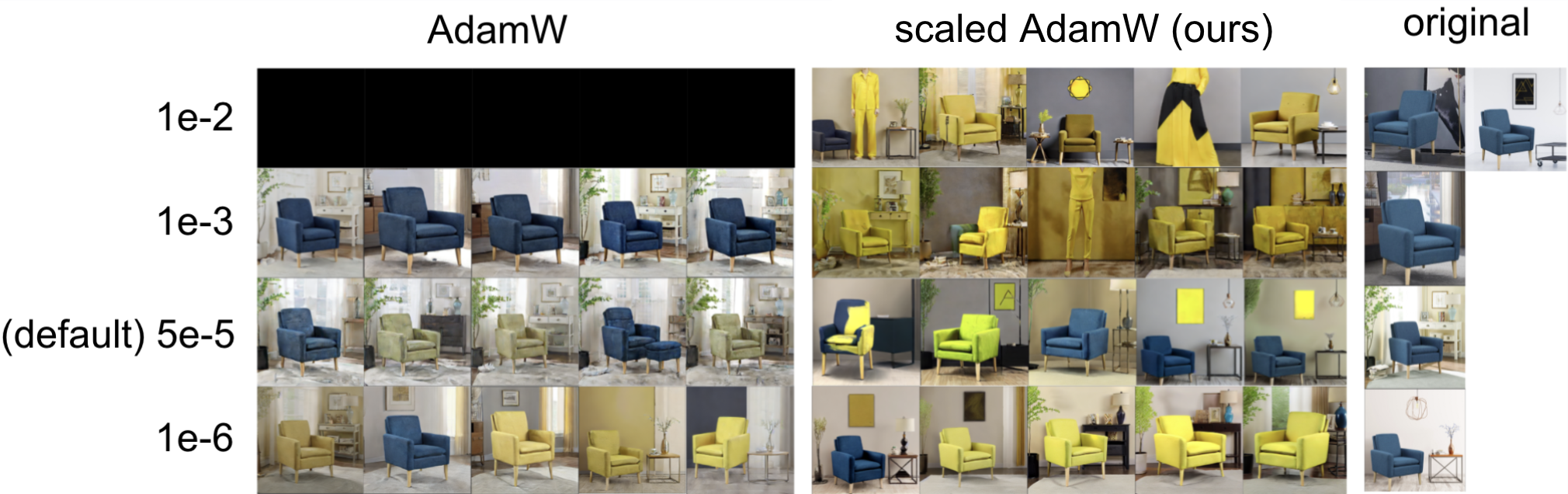
Figure 5: Generation results for prompt “a yellow $\langle TOK\rangle$” after fine-tuning on $5$ blue chair images of the Stable Diffusion V1.5 model. We vary text-encoder learning rates with U-Net learning rate fixed to default value $1e-4.$ No black images are observed for our method’s generation and AdamW generates only black images for large learning rates. Our method (scaled AdamW) generates photos better capturing the prompt and is more robust to learning rate changes. See Appendix D.1 for experimental details.

Figure 6: Generation results for prompt “$\langle TOK\rangle$ wearing a hat” after fine-tuning on $5$ dog images of the Stable Diffusion V1.5 model. See Appendix D.1 for experimental details. Our method (scaled AdamW) generates images better capturing the prompt, i.e., a dog wearing a hat, and is more robust to learning rate changes.

D.2 Mix-of-Show

For our experiment for face generation tasks, we base our experiments on Mix-of-Show (Gu et al., 2023) repository which we find able to generate high-quality face images and is better for visualization comparison between different optimization methods we consider. We follow default settings for training and inference in (Gu et al., 2023) with the exception that we turn off embedding tuning and only tune the text encoder and U-Net fraction where LoRA parameters are injected. The reason is that we find with embedding tuning, the effect of LoRA parameter is restricted and thus does no good to our comparison. In Mix-of-Show, Chilloutmix is used as pretrained model. LoRA rank is set to $4$. DMP-Solver (Lu et al., 2022) is employed for sampling. See (Gu et al., 2023) for more discussion on experimental details. Here we first fix step size $5e-4$ for both text encoder tuning and U-Net tuning and compare AdamW versus scaled AdamW with different LoRA parameter fusion coefficients. The default step size value used for Mix-of-Show is $1e-5$ and $1e-4$ for text encoder tuning and U-Net tuning respectively and default optimizer is AdamW. See Section D.2.1 for experimental results for different LoRA parameter fusion coefficients. Our scaled AdamW optimizer generates visually better images compared to AdamW optimizer. We then test with varying step size settings and demonstrate that our scaled gradient method is more robust to step size changes in Section D.2.2.

D.2.1 AdamW vs. scaled AdamW with varying LoRA parameter fusion coefficients

We experiment with Potter character and Hermione character. For Potter character, we use 14 Potter images for training LoRA parameters with the character name replace by special token $\langle TOK\rangle$ as what has been introduced in textual inversion (Gal et al., 2022), then in the sampling procedure, we use prompt with special character $\langle TOK\rangle$ for generating images involving Potter character. Figure 7, 8 and 9 show the generation results for three different prompts. The above two rows are for AdamW optimizer with the first row having LoRA parameter fusion coefficient $0.7$ and second row $1$ and the third and fourth rows correspond to scaled AdamW generation. LoRA parameter fusion coefficient represents $\alpha$ in $W=W_{0}+\alpha AB^{T}$ when merging LoRA weights. We observe that our scaled AdamW method is able to generate higher quality images compared to unscaled version for both $\alpha=0.7$ and $\alpha=1$. For Hermione character, we train with $15$ photos of Hermione following procedure described before. Figure 10 and 11 show the generation results. Still, our scaled AdamW optimizer produces higher quality images compared to AdamW optimizer.

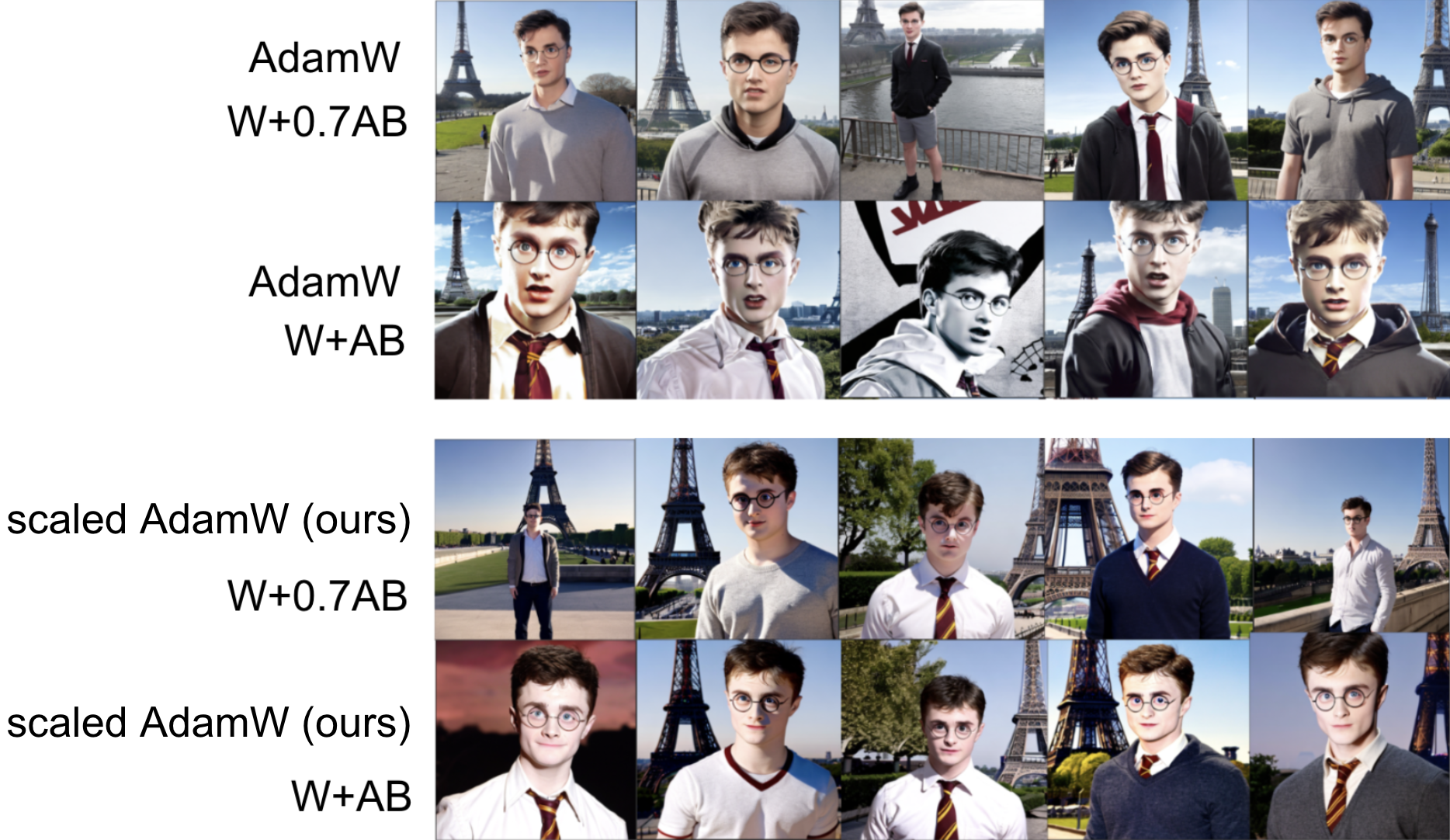
Figure 7: Generation results for prompt “a $\langle TOK\rangle$ in front of eiffel tower” after fine-tuning on $14$ Potter images. The above two rows are from AdamW optimizer and the bottom two rows are from our scaled AdamW optimizer. The first and third rows correspond to LoRA parameter fusion coefficient $0.7$ and the second and fourth rows correspond to LoRA parameter fusion coefficient $1.0$. Our scaled AdamW method generates images of higher quality compared to AdamW. See Appendix D.2.1 for experimental details.

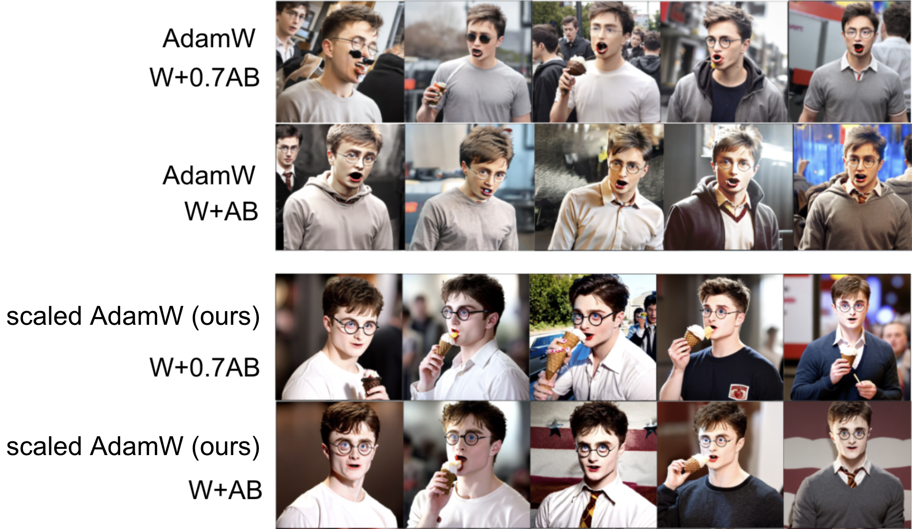
Figure 8: Generation results for prompt “$\langle TOK\rangle$ eating an icecream ” after fine-tuning on $14$ Potter images. The above two rows are from AdamW optimizer and the bottom two rows are from our scaled AdamW optimizer. The first and third rows correspond to LoRA parameter fusion coefficient $0.7$ and the second and fourth rows correspond to LoRA parameter fusion coefficient $1.0$. Our scaled AdamW method generates images of higher quality compared to AdamW. See Appendix D.2.1 for experimental details.

Figure 9: Generation results for prompt “$\langle TOK\rangle$” after fine-tuning on $14$ Potter images. The above two rows are from AdamW optimizer and the bottom two rows are from our scaled AdamW optimizer. The first and third rows correspond to LoRA parameter fusion coefficient $0.7$ and the second and fourth rows correspond to LoRA parameter fusion coefficient $1.0$. Our scaled AdamW method generates images of higher quality compared to AdamW. See Appendix D.2.1 for experimental details.

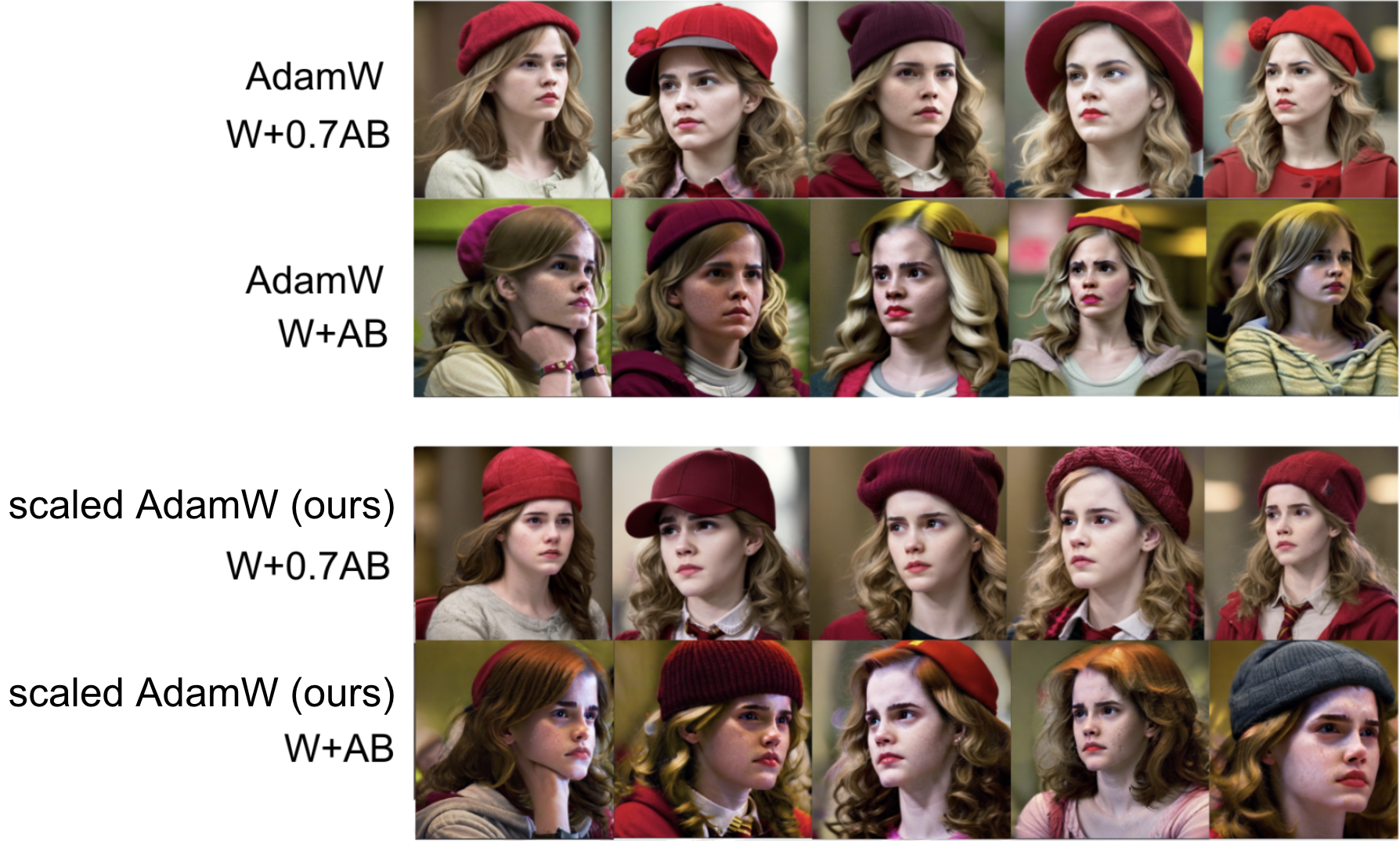
Figure 10: Generation results for prompt “$\langle TOK\rangle$ wearing a red hat” after fine-tuning on $15$ Hermione images. The above two rows are from AdamW optimizer and the bottom two rows are from our scaled AdamW optimizer. The first and third rows correspond to LoRA parameter fusion coefficient $0.7$ and the second and fourth rows correspond to LoRA parameter fusion coefficient $1.0$. Our scaled AdamW method generates images of higher quality compared to AdamW. See Appendix D.2.1 for experimental details.

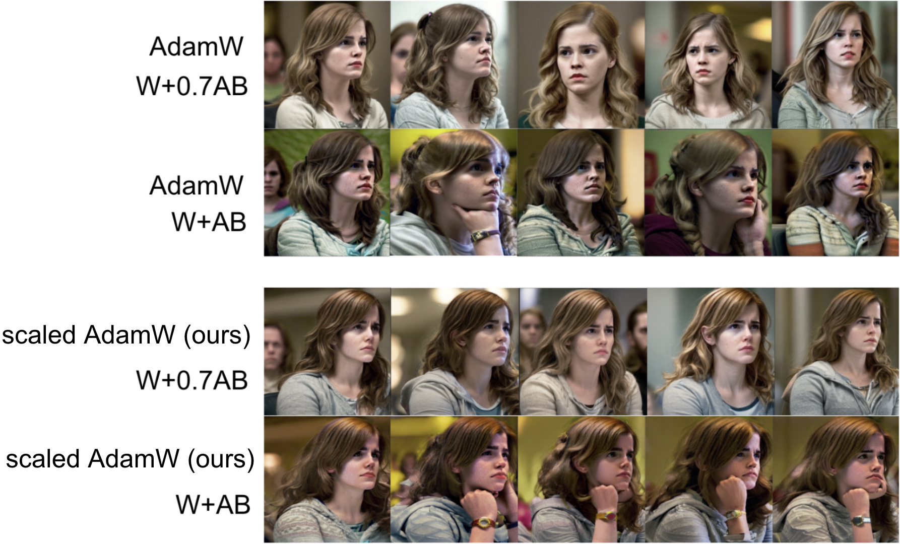
Figure 11: Generation results for prompt “$\langle TOK\rangle$” after fine-tuning on $15$ Hermione images. The above two rows are from AdamW optimizer and the bottom two rows are from our scaled AdamW optimizer. The first and third rows correspond to LoRA parameter fusion coefficient $0.7$ and the second and fourth rows correspond to LoRA parameter fusion coefficient $1.0$. Our scaled AdamW method generates images of higher quality compared to AdamW. See Appendix D.2.1 for experimental details.

D.2.2 Varying step sizes

Here we test with varying step sizes. Note the Mix-of-Show repository uses AdamW as default optimizer with learning rate $1e-5$ for text-encoder tuning and $1e-4$ for U-Net tuning. SGD method is not used in original repository. We emprically observe that SGD requires larger learning rate compared to AdamW to generate sensible images. For this experiment, we test with three groups of learning rates, with “Large” corresponds to $3e-1$ for SGD-type methods and $5e-4$ for AdamW-type methods; “Medium” corresponds to $1e-1$ for SGD-type methods and $1e-4$ for AdamW-type methods; “Small” corresponds to $5e-2$ for SGD-type methods and $1e-5$ for AdamW-type methods. We don’t differentiate learning rates for U-Net and text-encoder tuning and the same learning rate is used for both. Note the default learning rate for AdamW falls between the “Medium” learning rate and the “Small” learning rate thus our learning rate choices are not random. Figure 12, 13 and 14 show the generation results for three different prompts. It can be observed that our scaled optimizers are more robust to learning rate changes.

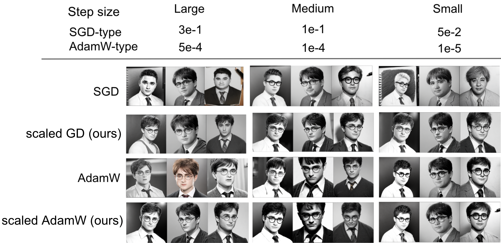
Figure 12: Generation results for prompt “a pencil sketch of $\langle TOK\rangle$” with different optimizers and different learning rates. See Appendix D.2.2 for experimental details. Default optimizer is AdamW with default learning rate $1e-4$ for U-Net tuning and $1e-5$ for text-encoder tuning. Our scaled optimizers generate better quality images and are more robust to learning rate changes.

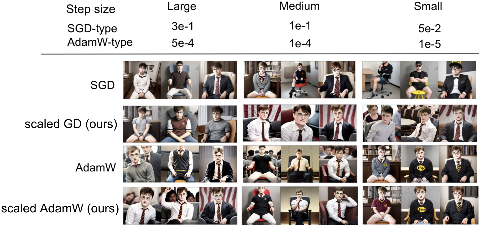
Figure 13: Generation results for prompt “$\langle TOK\rangle$ sit on the chair” with different optimizers and different learning rates. See Appendix D.2.2 for experimental details. Default optimizer is AdamW with default learning rate $1e-4$ for U-Net tuning and $1e-5$ for text-encoder tuning. Our scaled optimizers generate better quality images and are more robust to learning rate changes.

Figure 14: Generation results for prompt “a photo of $\langle TOK\rangle$” with different optimizers and different learning rates. See Appendix D.2.2 for experimental details. Default optimizer is AdamW with default learning rate $1e-4$ for U-Net tuning and $1e-5$ for text-encoder tuning. Our scaled optimizers generate better quality images and are more robust to learning rate changes.

References

- Candes et al. (2009) Candes, E. J., Li, X., Ma, Y., and Wright, J. Robust principal component analysis?, 2009.
- Chavan et al. (2023) Chavan, A., Liu, Z., Gupta, D., Xing, E., and Shen, Z. One-for-all: Generalized lora for parameter-efficient fine-tuning, 2023.
- Dettmers et al. (2023) Dettmers, T., Pagnoni, A., Holtzman, A., and Zettlemoyer, L. Qlora: Efficient finetuning of quantized llms, 2023.
- Duchi et al. (2011) Duchi, J., Hazan, E., and Singer, Y. Adaptive subgradient methods for online learning and stochastic optimization. Journal of Machine Learning Research, 12(61):2121–2159, 2011. URL http://jmlr.org/papers/v12/duchi11a.html.
- Gal et al. (2022) Gal, R., Alaluf, Y., Atzmon, Y., Patashnik, O., Bermano, A. H., Chechik, G., and Cohen-Or, D. An image is worth one word: Personalizing text-to-image generation using textual inversion, 2022.
- Gardent et al. (2017) Gardent, C., Shimorina, A., Narayan, S., and Perez-Beltrachini, L. The WebNLG challenge: Generating text from RDF data. In Alonso, J. M., Bugarín, A., and Reiter, E. (eds.), Proceedings of the 10th International Conference on Natural Language Generation, pp. 124–133, Santiago de Compostela, Spain, September 2017. Association for Computational Linguistics. doi: 10.18653/v1/W17-3518. URL https://aclanthology.org/W17-3518.
- Gu et al. (2023) Gu, Y., Wang, X., Wu, J. Z., Shi, Y., Chen, Y., Fan, Z., Xiao, W., Zhao, R., Chang, S., Wu, W., Ge, Y., Shan, Y., and Shou, M. Z. Mix-of-show: Decentralized low-rank adaptation for multi-concept customization of diffusion models, 2023.
- Gupta et al. (2018) Gupta, V., Koren, T., and Singer, Y. Shampoo: Preconditioned stochastic tensor optimization, 2018.
- Hu et al. (2021) Hu, E. J., Shen, Y., Wallis, P., Allen-Zhu, Z., Li, Y., Wang, S., Wang, L., and Chen, W. Lora: Low-rank adaptation of large language models, 2021.
- Huggingface team (2023) Huggingface team. Huggingface transformers documentation, 2023. URL https://huggingface.co/docs/transformers/main_classes/trainer. Accessed: 2024-01-25.
- Jia et al. (2023) Jia, X., Wang, H., Peng, J., Feng, X., and Meng, D. Preconditioning matters: Fast global convergence of non-convex matrix factorization via scaled gradient descent. In Thirty-seventh Conference on Neural Information Processing Systems, 2023.
- Jiang et al. (2023) Jiang, A. Q., Sablayrolles, A., Mensch, A., Bamford, C., Chaplot, D. S., de las Casas, D., Bressand, F., Lengyel, G., Lample, G., Saulnier, L., Lavaud, L. R., Lachaux, M.-A., Stock, P., Scao, T. L., Lavril, T., Wang, T., Lacroix, T., and Sayed, W. E. Mistral 7b, 2023.
- Kingma & Ba (2017) Kingma, D. P. and Ba, J. Adam: A method for stochastic optimization, 2017.
-
Labonne (2024)
Labonne, M.
Mistral fine-tuning example, 2024.
URL https://towardsdatascience.com/fine-tune-a-mistral-7b-model
-with-direct-preference-optimization
-708042745aac. Accessed: 2024-01-25. - Liu et al. (2023) Liu, W., Qiu, Z., Feng, Y., Xiu, Y., Xue, Y., Yu, L., Feng, H., Liu, Z., Heo, J., Peng, S., Wen, Y., Black, M. J., Weller, A., and Schölkopf, B. Parameter-efficient orthogonal finetuning via butterfly factorization, 2023.
- Loshchilov & Hutter (2019) Loshchilov, I. and Hutter, F. Decoupled weight decay regularization, 2019.
- Lu et al. (2022) Lu, C., Zhou, Y., Bao, F., Chen, J., Li, C., and Zhu, J. Dpm-solver: A fast ode solver for diffusion probabilistic model sampling in around 10 steps, 2022.
- Ma et al. (2023) Ma, C., Xu, X., Tong, T., and Chi, Y. Provably accelerating ill-conditioned low-rank estimation via scaled gradient descent, even with overparameterization, 2023.
- Mishkin et al. (2022) Mishkin, A., Sahiner, A., and Pilanci, M. Fast convex optimization for two-layer relu networks: Equivalent model classes and cone decompositions, 2022.
- Mishra & Sepulchre (2016) Mishra, B. and Sepulchre, R. Riemannian preconditioning. SIAM Journal on Optimization, 26(1):635–660, January 2016. ISSN 1095-7189. doi: 10.1137/140970860. URL http://dx.doi.org/10.1137/140970860.
- Mishra et al. (2012) Mishra, B., Apuroop, K. A., and Sepulchre, R. A riemannian geometry for low-rank matrix completion, 2012.
- Mistral AI team (2023) Mistral AI team. Mistral-7b announcement, 2023. URL https://mistral.ai/news/announcing-mistral-7b. Accessed: 2024-01-25.
- Nan et al. (2021) Nan, L., Radev, D., Zhang, R., Rau, A., Sivaprasad, A., Hsieh, C., Tang, X., Vyas, A., Verma, N., Krishna, P., Liu, Y., Irwanto, N., Pan, J., Rahman, F., Zaidi, A., Mutuma, M., Tarabar, Y., Gupta, A., Yu, T., Tan, Y. C., Lin, X. V., Xiong, C., Socher, R., and Rajani, N. F. DART: Open-domain structured data record to text generation. In Toutanova, K., Rumshisky, A., Zettlemoyer, L., Hakkani-Tur, D., Beltagy, I., Bethard, S., Cotterell, R., Chakraborty, T., and Zhou, Y. (eds.), Proceedings of the 2021 Conference of the North American Chapter of the Association for Computational Linguistics: Human Language Technologies, pp. 432–447, Online, June 2021. Association for Computational Linguistics. doi: 10.18653/v1/2021.naacl-main.37. URL https://aclanthology.org/2021.naacl-main.37.
- Pilanci & Ergen (2020) Pilanci, M. and Ergen, T. Neural networks are convex regularizers: Exact polynomial-time convex optimization formulations for two-layer networks, 2020.
- Puzikov & Gurevych (2018) Puzikov, Y. and Gurevych, I. E2E NLG challenge: Neural models vs. templates. In Krahmer, E., Gatt, A., and Goudbeek, M. (eds.), Proceedings of the 11th International Conference on Natural Language Generation, pp. 463–471, Tilburg University, The Netherlands, November 2018. Association for Computational Linguistics. doi: 10.18653/v1/W18-6557. URL https://aclanthology.org/W18-6557.
- Qiu et al. (2023) Qiu, Z., Liu, W., Feng, H., Xue, Y., Feng, Y., Liu, Z., Zhang, D., Weller, A., and Schölkopf, B. Controlling text-to-image diffusion by orthogonal finetuning, 2023.
- Radford et al. (2019) Radford, A., Wu, J., Child, R., Luan, D., Amodei, D., and Sutskever, I. Language models are unsupervised multitask learners. 2019. URL https://api.semanticscholar.org/CorpusID:160025533.
- Recht et al. (2010) Recht, B., Fazel, M., and Parrilo, P. A. Guaranteed minimum-rank solutions of linear matrix equations via nuclear norm minimization. SIAM Review, 52(3):471–501, January 2010. ISSN 1095-7200. doi: 10.1137/070697835. URL http://dx.doi.org/10.1137/070697835.
- Rombach et al. (2022) Rombach, R., Blattmann, A., Lorenz, D., Esser, P., and Ommer, B. High-resolution image synthesis with latent diffusion models. In Proceedings of the IEEE/CVF Conference on Computer Vision and Pattern Recognition (CVPR), pp. 10684–10695, June 2022.
- Ryu (2023) Ryu, S. Low-rank adaptation for fast text-to-image diffusion fine-tuning. https://github.com/cloneofsimo/lora/tree/master, 2023.
- Stanley et al. (2004) Stanley, R. P. et al. An introduction to hyperplane arrangements. Geometric combinatorics, 13(389-496):24, 2004.
- Tong et al. (2021a) Tong, T., Ma, C., and Chi, Y. Low-rank matrix recovery with scaled subgradient methods: Fast and robust convergence without the condition number. IEEE Transactions on Signal Processing, 69:2396–2409, 2021a. ISSN 1941-0476. doi: 10.1109/tsp.2021.3071560. URL http://dx.doi.org/10.1109/TSP.2021.3071560.
- Tong et al. (2021b) Tong, T., Ma, C., and Chi, Y. Accelerating ill-conditioned low-rank matrix estimation via scaled gradient descent, 2021b.
- Tong et al. (2022) Tong, T., Ma, C., Prater-Bennette, A., Tripp, E., and Chi, Y. Scaling and scalability: Provable nonconvex low-rank tensor estimation from incomplete measurements, 2022.
- Valipour et al. (2023) Valipour, M., Rezagholizadeh, M., Kobyzev, I., and Ghodsi, A. Dylora: Parameter efficient tuning of pre-trained models using dynamic search-free low-rank adaptation, 2023.
- Wang et al. (2018) Wang, A., Singh, A., Michael, J., Hill, F., Levy, O., and Bowman, S. GLUE: A multi-task benchmark and analysis platform for natural language understanding. In Linzen, T., Chrupała, G., and Alishahi, A. (eds.), Proceedings of the 2018 EMNLP Workshop BlackboxNLP: Analyzing and Interpreting Neural Networks for NLP, pp. 353–355, Brussels, Belgium, November 2018. Association for Computational Linguistics. doi: 10.18653/v1/W18-5446. URL https://aclanthology.org/W18-5446.
- Zhang et al. (2023a) Zhang, F. F., Li, L., Chen, J.-C., Jiang, Z., Wang, B., and Qian, Y. Increlora: Incremental parameter allocation method for parameter-efficient fine-tuning. ArXiv, abs/2308.12043, 2023a. URL https://api.semanticscholar.org/CorpusID:261076438.
- Zhang et al. (2023b) Zhang, G., Chiu, H.-M., and Zhang, R. Y. Fast and minimax optimal estimation of low-rank matrices via non-convex gradient descent, 2023b.
- Zhang et al. (2023c) Zhang, G., Fattahi, S., and Zhang, R. Y. Preconditioned gradient descent for overparameterized nonconvex burer–monteiro factorization with global optimality certification, 2023c.
- Zhang et al. (2023d) Zhang, Q., Chen, M., Bukharin, A., He, P., Cheng, Y., Chen, W., and Zhao, T. Adaptive budget allocation for parameter-efficient fine-tuning, 2023d.
- Zi et al. (2023) Zi, B., Qi, X., Wang, L., Wang, J., Wong, K.-F., and Zhang, L. Delta-lora: Fine-tuning high-rank parameters with the delta of low-rank matrices, 2023.