On Secure mmWave RSMA Systems††thanks: Manuscript received.
Abstract
Millimeter-wave (mmWave) communication is one of the effective technologies for the next generation of wireless communications due to the enormous amount of available spectrum resources. Rate splitting multiple access (RSMA) is a powerful multiple access, interference management, and multi-user strategy for designing future wireless networks. In this work, a multiple-input-single-output mmWave RSMA system is considered wherein a base station serves two users in the presence of a passive eavesdropper. Different eavesdropping scenarios are considered corresponding to the overlapped resolvable paths between the main and the wiretap channels under the considered transmission schemes. The analytical expressions for the secrecy outage probability (SOP) are derived respectively through the Gaussian–Chebyshev quadrature method. Monte Carlo simulation results are presented to validate the correctness of the derived analytical expressions and demonstrate the effects of system parameters on the SOP of the considered mmWave RSMA systems.
Index Terms:
Millimeter-wave, rate splitting multiple access, uniform linear array, secrecy outage probability.I Introduction
I-A Background and Related Work
Nowadays, a growing number of electronic devices and various emerging applications have entered our daily routines, which bring about significant growth in the wireless data traffic of wireless networks and is likely to leap 10000 fold in the next 20 years [1]-[3]. To tackle this incredible growth, millimeter-wave (mmWave) has become one of the most efficient resolutions due to the plentiful underutilized spectrum resources [4]. Recently, mmWave communication has received substantial attention, such as channel modelling and estimation, beamforming strategy design, and performance analysis. The authors in [5] provided a comprehensive overview of mathematical models and analytical techniques of mmWave cellular systems. A baseline mathematical method and analysis in blocking and substantial directionality aspects was proposed and the result indicated that the ultra-dense deployments were more available in mmWave systems. In [6], an adaptive algorithm was developed to estimate the mmWave channel parameters exploiting the sparse scattering of the channel and was extended to the case of the multi-path channel. The result shows that the proposed low-complexity channel estimation algorithm achieves more precoding gains and spectral efficiency than exhaustive algorithms. In [7], a hybrid precoding/combining designs of full-duplex amplify-and-forward mmWave relay systems was proposed. Their simulation indicated that the proposed design is approaching an all-digital scheme. A downlink non-orthogonal multiple access (NOMA) mmWave system was investigated in [8]. An opportunistic beam-splitting NOMA scheme was proposed to inquire into the antenna gain and the closed-form expressions of the coverage probability and the ASR were derived.
In next-generation communication networks and beyond, interference management becomes a fundamental problem for multi-user communications and multiple access design [9]. Rate-splitting multiple access (RSMA) as a candidate multiple access scheme has been proposed in [10] and has been recognized as a powerful multiple access, interference management, and multi-user strategy [11]. Based on the rate-splitting (RS) principle, RSMA not only displays more flexibility in managing interference, i.e., partially decodes interference of inter-user and partially treats interference as noise, but also unifies and generalizes orthogonal multiple access (OMA), space-division multiple access, NOMA, physical-layer multicasting [12], [13], [14]. A more flexible and powerful cooperative scheme for a multiple-input-single-output (MISO) broadcast channel scenario was proposed based on the three-node relay channel in [15]. Their simulation results show that the proposed cooperative RS strategy can obtain an explicit rate improvement than NOMA. In [16], linearly-precoded 1-layer and multi-layer transmission strategies based on the RS were investigated in a Non-Orthogonal unicast and multicast transmission system, which the weighted sum rate and energy efficiency problems were solved by weighted minimum mean square error algorithm and successive convex approximation algorithm. The Numerical results indicated that the RS-assisted transmission strategies are more efficient in spectrum and energy compared with multi-user linear- precoding, OMA and NOMA in extensive user deployments and network loads. Compared to rate region, sum rate, spectral and energy efficiency improvement in terms of optimization, the benefit of RSMA for performance analysis, such as throughput, ergodic sum rate (ESR), and outage probability (OP), also needs to be explored. In [17], the downlink unmanned aerial vehicle systems based on the RSMA scheme were investigated and the closed-form expressions of the OP and throughput at each user were derived. The performance of a multi-cell RSMA network was investigated in [18] wherein the analytical expressions for ESR and spectral efficiency based on stochastic geometry theory were derived. Their results showed that the power splitting ratio between common and private streams significantly impacts performance. Bansal A. et al. in [19] studied a novel Intelligent reflecting surface (IRS) RS framework of multi-user communication system, the closed-form expressions of OP for the far and near users were derived. The simulation results showed that the proposed framework was superior to the decode-and-forward-RS, RS without IRS, and IRS-NOMA scenarios.
Physical layer security (PLS), which utilizes the inherent characteristics of wireless channels, is an exciting complement to sophisticated cryptographic techniques [20]. Since the mmWave’s propagation characteristics, which support large antenna arrays and highly directional transmission, can reduce the leakage of confidential information. Thus, physical layer security in mmWave communications has attracted considerable recent attention. Specifically, by using a sectored model to analyze the beam pattern, the secrecy transmission of a mmWave cellular network was investigated in [21], the secure connectivity probability was studied and their results indicated the array pattern and intensity of eavesdroppers are both important network parameters for improving the secrecy performance. The author studied the physical layer security of mmWave relaying networks In [22] wherein developed a new joint relay selection and power allocation method in multiple eavesdroppers and relays, the closed-form expressions of average secrecy rate (ASR) and secrecy outage probability (SOP) were derived respectively and demonstrated the superiority of proposed method. Ju et al. in [23] utilized the discrete angular domain channel (DADC) model to analyze the secrecy performance of the mmWave MISO systems. Three transmission schemes were proposed to improve the secure mmWave systems. Further, they investigated the security mmWave MISO systems in the presence of multiple randomly located eavesdroppers in [24]. In [25], the multiple input multiple output DADC were developed in mmWave decode-and-forward relay systems. The secrecy performance with three eavesdropping scenarios was investigated by designing the corresponding beamforming strategies. Huang et al. investigated the secure mmWave NOMA systems in which all the authorized and unauthorized receivers were randomly located in [26]. Then, they proposed two schemes to improve the secrecy transmission and the closed-form SOPs for two beamforming schemes with varying eavesdropper detection abilities were derived.
As a novel, general, and robust framework for the sixth generation mobile communications, RSMA has a high potential to be used for security applications [27]. In [28], two decoding strategies were adopted by a near user and a far user to explore outage and secrecy outage performance. The closed-form expressions of OP and tight approximations of SOP were derived, considering four decoding combinations. The author in [29] proposed two RS schemes with one-layer-successive interference cancellation (SIC) and two-layer-SIC wherein there is an untrusted near user. The closed-form expressions of OP and SOP are obtained to analyze outage performance. In [30], the secrecy performance of RSMA in multi-user MISO systems was investigated and analytical expressions of the ESR and ASR were obtained with zero-forcing precoding and minimum mean square error approach. The result demonstrated that proposed power allocation methods could offer inherent tradeoffs over the ESR and ASR.
In the RSMA scheme, the messages are split into common and private parts, encoded into a single common stream and private streams, respectively. All the common and private streams are superimposed, linearly precoded, and transmitted simultaneously by the transmitter. By utilizing SIC technology, the common stream is decoded firstly by treating all private streams as interference, removing from the received signals, and the private stream is decoded by treating the private streams for other users as interference. In the mmWave systems with the DADC model, depending on the spatial correlation of the users, the spatially resolvable paths are split into overlapped and non-overlapped paths. As thus, the following questions naturally arise: Should the common streams be transmitted on overlapped paths or all paths? What is the performance of the mmWave systems with the RSMA scheme? To answer these questions, the performance of the mmWave RSMA systems was investigated, and two beamforming transmission schemes were proposed in [32]. The closed-form expressions for the exact and asymptotic OP with proposed schemes were derived using stochastic geometry theory. The results demonstrated that RSMA helps improve transmission reliability of the mmWave systems. TABLE I outlines the typical works discussed.
| Reference | RSMA | mmWave | Multi-antenna technology | Channel Model | PLS | Performance metric |
| [17] | ✓ | Nakagami- | OP | |||
| [18] | ✓ | Transmitter | Rayleigh | ESR | ||
| [19] | ✓ | Rayleigh | OP | |||
| [21] | ✓ | Nakagami- | ✓ | SCP | ||
| [22] | ✓ | Transmitter | Rayleigh | ✓ | SOP | |
| [23] | ✓ | Transmitter | DADC | ✓ | SOP | |
| [24] | ✓ | Transmitter | DADC | ✓ | SOP | |
| [25] | ✓ | Transmitter & destination | DADC | ✓ | SOP | |
| [26] | ✓ | Transmitter | DADC | ✓ | SOP | |
| [28] | ✓ | Rayleigh | ✓ | OP and SOP | ||
| [29] | ✓ | Transmitter | Rayleigh | ✓ | OP and SOP | |
| [30] | ✓ | Transmitter | Rayleigh | ✓ | ESR & ASR | |
| [32] | ✓ | ✓ | Transmitter | DADC | OP | |
| Our Work | ✓ | ✓ | Transmitter | DADC | ✓ | SOP |
I-B Motivation and Contributions
To the best of the authors’ knowledge, based on the open literature, there is a lack of research focused on the following issue: Is it beneficial to leverage the RSMA scheme in mmWave systems for security enhancement? Hence, this work answers this question by analyzing the secrecy performance of the mmWave RSMA systems. Different eavesdropping scenarios are considered corresponding to the overlapped resolvable paths between the main and the wiretap channels under the considered transmission schemes. Technically speaking, it is much more challenging to obtain the analytical expression of the SOP than that of the OP for the mmWave RSMA system since there are multiple parameters (random variables) that must be considered. We summarize the contributions of this work as follows.
-
1.
The secrecy performance of the MISO mmWave RSMA system is investigated wherein the common and private streams are transmitted on the overlapping and non-overlapping paths, respectively. Different scenarios are considered based on the spatial correlation of the legitimate and illegitimate user and the principle of the RSMA scheme. Subsequently, the analytical expressions for the SOP are derived respectively through the Gaussian–Chebyshev quadrature method.
-
2.
We present Monte Carlo simulation results to validate the correctness of the derived analytical expressions and demonstrate the effects of system parameters on the SOP of the considered mmWave RSMA systems. The result shows that the power allocation between the common and private streams and the number of overlapped paths significantly affect the secrecy performance.
-
3.
Relative to [26] wherein the security mmWave NOMA systems were enhanced by the proposed beamforming schemes, the security mmWave RSMA system is improved by the proposed beamforming scheme in this work wherein the scenarios considered in this work are more challenging.
-
4.
Relative to [28]-[31] wherein the secrecy performance of the RSMA systems with internal untrusted users was investigated. In these scenarios, it was assumed that the common message could always be decoded and only the private message was wiretapped. Technically speaking, it is much more challenging to investigate the secrecy performance of the RSMA systems with an external eavesdropper than with an internal eavesdropper.
I-C Organization
The rest of this paper is organized as follows. Section II describes the system model and beamforming scheme. The analytical expressions for the exact SOP of mmWave RSMA systems is derived under different scenarios in Sections III. The simulation results are presents to valid the analysis in Section IV. Section V concludes this work. Table II lists the notations and symbols utilized throughout this work.
| Notation | Description |
| The index set of resolvable paths at | |
| The complex gain vector between and | |
| The spatially orthogonal basis | |
| The number of resolvable paths of | |
| The angular range between the th and th paths at | |
| The width between the th and th paths at | |
| The index set of overlapped paths between and | |
| The index set of non-overlapping paths at | |
| The index set of overlapped paths among and | |
| The index set of overlapped paths between and | |
| The power allocation coefficient for | |
| The power allocation coefficient for | |
| The secrecy rate threshold for the common messages | |
| The secrecy rate threshold for the private messages | |
| Meijer’s -function | |
| Extended generalized bivariate Fox’s -function | |
| Gamma function | |
II System Model
II-A System Model

As shown in Fig. 1, a downlink mmWave RSMA system is considered where the base station communicates with two users denoted by and 111 Similar to [10], [12], [14], the RSMA system with two users is considered in this work. As such, the results in this paper can serve as a benchmark for the performance of such systems. The performance of RSMA systems with multiple users will be part of our future work. while an external passive eavesdropper denoted by attempt to intercept the information. is equipped with antennas and both legitimate and illegitimate receivers are equipped with a single antenna.
Similar to [32], the message, , is split into and . and are encoded together into , which is a common stream decoded by both users. At the same time, and are encoded into and , respectively. The transmitted signal from is given by
| (1) |
where , , and are unit vectors that denote the beamforming direction, signifies the transmit power, and and denote the power allocation coefficient for and , respectively.
The polar coordinate system is established with the position of as the origin. The position of and are expressed as and respectively, where is the center angle of angles of departure (AODs) of ’s paths, i.e., . The channels of between and the receiver is expressed as [23]-[25]
| (2) |
where , , , , GHz [35], denotes the distance between the transmitter and the receiver , signifies the path loss exponent, denotes the number of resolvable paths of the receiver , is the spatially orthogonal basis, . It is assumed that the AODs of the receiver ’ paths is distributed within the angular range , where if otherwise [23]. To facilitate analysis, we assumed that and . We define sets . So we have , where . Define the angular range and the width , where () describes the angular range of user between the th and th spatially resolvable paths, denote the width between the th and th spatially resolvable paths.. Then we have .
Based on the spatial correlation of all receivers, the spatially resolvable paths are divided into overlapped and non-overlapping paths [23]. and are defined as the number of the overlapped and non-overlapping paths between and , respectively. Thus, we have , , . , and . Similarly, , , denote the number of the overlapped paths between , and , , , respectively. Thus, we have and , , , , .
In this work, is transmitted on the overlapped paths and is transmitted on their non-overlapping paths to eliminate the inter-user interference of private signals by utilizing the spatial correlation of two users’ channels [32]. Similar to [23] and [32], it is assumed that the perfect channel state information (CSI) of the legitimate receivers is available at , the beamforming for is expressed as , where is utilized to generate a new matrix with columns selected from based on the selected column index set , and denotes the index sets of common resolvable paths between the receiver and . Similarly, the beamforming for is expressed as , where denotes the index set of the non-overlapping paths of receiver . Thus, the transmitted signal from is rewritten as
| (3) |
where and .
II-B Signal to Interference Plus Noise Ratio
According to the RSMA principle, decodes firstly by treating all the other signals as noise. Then the instantaneous signal-to-interference and noise ratio (SINR) of decoding at is , where , , , and . After performing SIC, i.e., is re-encoded, precoded, and removed from the received signal, the SINR of decoding at is obtained as .
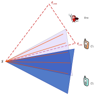
In this work, it is assumed that is interested only in ’s message 222 Since the analysis for both users is interchangeable, the secrecy performance of the scenarios in which is interested in ’s message can be obtained based on the results of this manuscript. . Moreover, for tractability of analysis, () is represented by , the users’ locations are assumed to be fixed in this work 333 The secrecy performance of scenarios wherein the users are randomly distributed also can be easily obtained based on [32, (7)] and the results of this work. . Depending on the relative positions of and , as shown in Fig. 2, there are four scenarios for the SINR of 444 Except for the four scenarios considered here, there is another scenario wherein there is no overlapped path between and and both the common and private messages are secure. , where signifies the angular range of between the th and th spatially resolvable paths, similarly, signifies the angular range of between the th and th spatially resolvable paths.
1) Scenario I:
As show in Fig. 2(a), only the private stream of is wiretapped by , which denotes . The SINR of in eavesdropping private stream of is given as where .
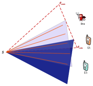
2) Scenario II:
This scenario is shown in Fig. 2(b), where in both common and private streams of are eavesdropped by . More Specifically, all non-overlapping resolvable paths of is wiretapped and overlapped paths of is partially wiretapped. Like [33], it is assumed that illegitimate has the same decoding capability as the legitimate users555 There is another eavesdropping scenario, called the worst-case security scenario, considered in many works, such as [33, 34]. Specifically, by utilizing specific detection techniques, the data stream received can be distinguished by the eavesdropper by subtracting interference generated by the superposed signals from each other. This assumption has been utilized in a reasonable amount of literature focused on the physical layer security of NOMA systems. In fact, this assumption simplified the analysis but overestimated the eavesdropper’s multi-user decodability. . According to the RSMA principle, decodes common streams of firstly by treating all the other signals as noise, and then decodes private streams of . Thus, the SINR of in eavesdropping both the common stream and private stream of are given as
| (4) |
| (5) |
respectively, where .
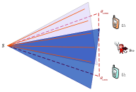
3) Scenario III:
As show in Fig. 2(c), all the overlapped paths and part of the non-overlapping paths for is intercepted. Similarly, the firstly decodes common streams and then decodes private streams of . Thus, the SINR of in eavesdropping the common stream and private stream of are given as
| (6) |
and
| (7) |
respectively, where .
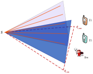
4) Scenario IV:
This case is shown in Fig. 2(d) wherein only the common stream of is eavesdropped by , which denotes and
| (8) |
To facilitate analysis, we define . The PDF and CDF of are expressed as
| (9) |
and
| (10) |
respectively, where , , , , and .
III Secrecy Outage Probability Analysis
In this work, is secure only when both the common and private stream are secrecy. Thus, the SOP of in the th scenario is expressed as
| (11) |
where denotes instantaneous secrecy capacity of common streams intended to , denotes instantaneous secrecy capacity of private streams transmitted to the , , and and signify the secrecy rate threshold for the common and private messages, respectively, and denotes the secrecy connection probability (SCP), which is the complementary of SOP. It should be noted that, when can only wiretap the common streams or private streams, the SCP of is degenerated to or respectively.
1) Scenario I:
In this case, only eavesdrop on private streams of . Based on (9), (10) and (11), utilizing [36, (3.351.3)], is obtained as
| (12) | ||||
where denotes the expectation operation, , , and .
2) Scenario II:
In this case, the private streams is eavesdropped completely while the common streams is partly eavesdropped. Thus, the SCP of is expressed as
| (13) | ||||
where , , , , . Based on (9) and (10) and utilizing [36, (3.351.2)], is obtained as
| (14) | ||||
where and . Define , , the PDF of is obtained as
| (15) |
Then, is obtained as
| (16) | ||||
where , and .
Utilizing [36, (3.351.2), (3.351.3)], is obtained as (17), shown at the top of this page, where . Similarly, based on (16) and utilizing [36, (7.811.5)] and (25.4.39), we obtain as (18), shown at the top of next page, where , , is the Meijer’s -function as defined by [36, (9.301)], is the summation items that reflect accuracy versus complexity, , , and .
| (17) | ||||
| (18) | ||||
3) Scenario III:
In this case, the common streams is eavesdropped completely while the private streams is eavesdropped partly. Thus, is expressed as
| (19) | ||||
where and , , and . Based on (9) and (10) and utilizing [36, (3.351.1)], is obtained as
| (20) | ||||
where . Substituting (20) into (19), is obtained as
| (21) | ||||
where
,
,
,
and
.
Utilizing [36, (3.351.2)], is obtained as
| (22) | ||||
Based on (10) and (15) and utilizing [36, (3.351.3), (7.811.5)], is obtained as
| (23) | ||||
where , , , , and . Based on (9) and (15), is obtained as
| (24) | ||||
where
and
,
.
Then, utilizing [36, (7.811.5)] and (25.4.39), is obtained as
| (25) | ||||
where , , and is the summation items that reflect accuracy versus complexity. Based on (25) and utilizing (25.4.45), is obtained as (26), shown at the top of next page, where is the summation items that reflect accuracy versus complexity, is the th zero of Leguerre polynomials and is Gaussian weight, which are given in Table (25.9) of [37]. With the same method, is obtained as
| (26) | ||||
| (27) |
where , . By utilizing [36, (7.811.5)] and (25.4.45), is obtained as as (28), shown at the top of next page, where , , , is the summation items that reflect accuracy versus complexity, is the th zero of Leguerre polynomials and is Gaussian weight, which are given in Table (25.9) of [37]. Based on (28) and utilizing (25.4.45), is obtained as
| (28) | ||||
| (29) | ||||
where , , is the summation items that reflect accuracy versus complexity, is the th zero of Leguerre polynomials and is Gaussian weight, which are given in Table (25.9) of [37].
4) Scenario IV:
In this case, only eavesdrop on common streams. It should noted that and are independent of each other in this case. Based on (9) and (10) and utilizing [36, (3.351.3)], the CDF of and PDF of are obtained as
| (30) |
| (31) | ||||
respectively, where and .
To facilitate the following analysis, we define
| (32) |
By utilizing [38, (10), (11)], [36, (9.31.5)], and [39, (1.2)] in turn, we obtain
| (33) | ||||
where is the extended generalized bivariate Fox’s H-function as defined by [39, (2.57)].
The SCP of in this scenario, is obtained as
| (34) | ||||
where
| (35) | ||||
and
| (36) | ||||
The analytical expressions provided in this section are complicated since many factors affect the secrecy performance of , specifically, the transmit power, power allocation coefficient, the target data rate, and relative locations between all the legitimate users and illegitimate receivers.
IV Numerical Results
This section presents simulation and numerical results to verify the secrecy outage performance of mmWave RSMA systems with the considered beamforming scheme. The noise power is set at dBm, and the path-loss model is set as [21, 25, 35]. In all the figures, ‘Sim’ and ‘Ana’ denote the simulation and numerical results, respectively.
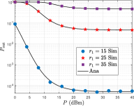
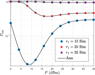
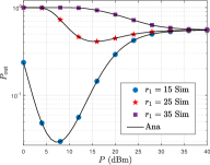
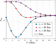
Fig. 3 demonstrates the impact of for varying on SOP. In Fig. 3(a), one can easily observe that the secrecy outage performance of the mmWave RSMA systems is enhanced while increasing . There is a floor for the SOP, which is independent of , which has been testified in [40] and stated in Remark 1. Furthermore, the SOP with lower outperforms that with larger since lower denotes weak path loss on . One interesting result is found from Fig.s 3(b) - 3(d) that the secrecy outage performance of initially decreases as increases and then increases to a constant. The reason is given as follows. In Fig. 3(b), part of the common stream and all the private streams are wiretapped, and decoding the common stream is the bottleneck in the scenarios with lower and decoding the private stream is the bottleneck in the scenarios with larger . However, in Fig. 3(c), all of the common stream and the private stream are wiretapped, and decoding the private stream is the bottleneck in all the scenarios. In Fig. 3(d), only part of the common stream is wiretapped. Moreover, it can be found that the SOP floor is independent of in the scenarios where the bottleneck is decoding the common stream. Based on all the subfigures in Fig. 3, we also find that the effect from the location of on the difference between the SOP of with different is weakening.
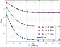
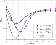
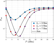
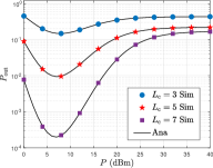
Fig. 4 presents the impact of for varying on the SOP of . In Fig. 4(a), one can observe the SOP increases as increases, which is easy to follow since more significant leads to less , thus, become smaller and transmissions become more vulnerable to intercept. In Figs. 4(b) and 4(c), one can observe that SOP initially decreases and then increases in the lower- region as increases, indicating an optimal in the lower- region to minimize the SOP of . This is because, in the scenarios with the lower , the SOP of depends on both the SINR/SNR of the common and private signals and decoding the common stream is the RSMA system’s bottleneck; thus, the larger the , the larger the , and the smaller SOP. In the scenarios with the larger , decoding the private signals is the RSMA system’s bottleneck, and the more significant leads to the smaller and the larger SOP. In Fig. 4(d), it can be observed that the secrecy performance of is improved as increases since larger leads to .
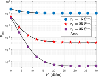
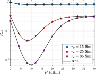
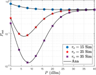
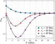
Fig. 5 demonstrates the impact of with varying on the SOP of . We observe that SOP decreases as increases; this is because the path loss of is the main factor affecting SOP. In the larger- region, SOP decreases as increases in Fig. 5(a) while SOP initially decreases and then increases as increases Figs. 5(b) - 5(d) with the same reason as in Figs. 3(a) - 3(d). In the low- region, we observe that SOP decreases as increases in all the cases, which denotes that more power can improve security performance.
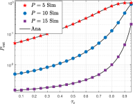
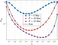
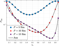
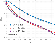
Fig. 6 plots the impact of with varying on the SOP of . We observe that SOP increases as in Fig. 6(a), which is easy to follow since less power is allocated to private streams as increasing . In Figs. 6(b) and 6(c), one can observe SOP initially decreases and then increases as increases, which denotes that there is an optimal to minimize the SOP. This is because in the lower- region, decoding the common streams is the bottleneck. Thus, increasing will enhance the secrecy outage performance. In the larger- region, decoding the private streams will be the bottleneck. However, the power allocated to the private stream decreases, so the SOP deteriorates. Moreover, the optimal is relative to and . Based on Fig. 6(d), the secrecy performance of improves with the increasing since the SINR of common streams at increases as .
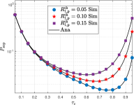
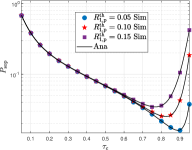
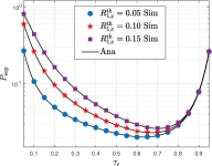
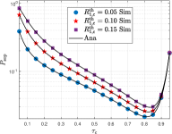
Fig. 7 presents the impact of with varying / on the SOP of . We observe that SOP decreases as / decreases, which is easy to follow since a more significant targeted secrecy rate denotes higher security requirements. Moreover, the optimal depends on /. The smaller /, the larger optimal , which is due to the low requirements and more power can be allocated to the stream to be the system’s bottleneck. In Figs. 7(a) and 7(b), in the large- region private signals is the bottleneck, so has a more pronounced impact on the SOP. However, in Figs. 7(c) and 7(d), in the lower- region common signals is the bottleneck, so has a more pronounced impact on SOP.
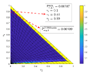
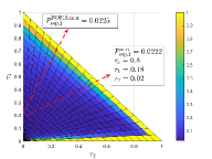
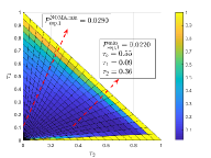
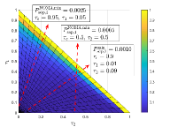
To evaluate the performance of the RSMA-based mmWave systems, NOMA-based mmWave systems is utilized as the benchmark in this work, which can be found in Fig. 8, wherein the SOP of for varying , , and is presented. Like [28], and represent the least achievable SOP of RSMA and NOMA systems, respectively. We observe that successively increases and then decreases from Figs. 8(a) - Fig. 8(d). The underlying reason is that the overlapped resolvable paths between and become larger initially, and then eavesdroppers can wiretap more confidential messages. Then, the overlapped resolvable paths between and become smaller and also interfered with by messages of ; thus, the secrecy performance of the mmWave RSMA system is improved. Fig. 8(a) indicated that in the case of significant differences of and , more power should be allocated to to improve secrecy performance. In Figs. 8(b) - 8(d), one can observe that the secrecy performance of common streams is easier to become a bottleneck; thus, larger and more minor can achieve better secrecy performance. In Figs. 8(c) and 8(d), a more significant fraction of power should be allocated to relative to to confuse the eavesdropper. If or in Figs. 8(a) - 8(c) is close to zero, the SOP would be close to 1 since with a low value of the users’ SINRs are not sufficient for decoding the common stream or private stream; When equals zero, the RSMA system will degenerate as a NOMA system. We observe that the is less than or equal to , the underlying reason in Figs. 8(b) - 8(c) is that common streams are easier to become a bottleneck. More power is allocated to in NOMA systems than RSMA systems, and the secrecy performance of common streams worsens as increases. In Fig. 8(d), when or is equal to zero, the RSMA system would degenerate as a NOMA system, one can observe that at is less than . In comparison, at is larger than , the reason is that as and directly makes increase and decrease.
Based on the results, some new insights are obtained as follows.
-
1.
In RSMA mmWave systems, both common and private streams can be the bottleneck of the security.
-
2.
There is an optimal transmit power to minimize the SOP of RSMA-based mmWave systems and the optimal transmit power depends on the overlapped paths and distances in the considered systems.
-
3.
There is an power allocation coefficient to minimize the SOP of RSMA-based mmWave systems and the optimal power allocation coefficient depends on many parameters, such as, the transmit power, target secrecy rates of common streams and private streams, relative location of all the receivers.
-
4.
Relative to Scenario I and Scenario II, allocating more power to than in Scenario III and Scenario IV can enhance ’s security.
V Conclusion
In this paper, the secure transmissions considering multipath propagation for mmWave RSMA MISO systems were analyzed. Based on the spatial correlation of the users and the eavesdropper, different eavesdropping scenarios were considered to investigate the secrecy performance, and then the analytical expressions of the SOP for four scenarios were derived. Our results illustrated the effects of overlapped paths between receivers, the power allocation coefficient of RSMA users, and channel parameters on the SOP of RSMA-based mmWave systems. This work considered that the illegitimate user has the same decode order according to the framework of the RSMA system. Other potential threats or more diverse eavesdropping strategies will be interesting work and part of the future work. Moreover, the results of this work demonstrate an optimal power allocation coefficient to minimize the SOP of RSMA systems. Thus, allocating power reasonably to the common and private streams is vital for the secure transmissions of RSMA mmWave systems. It is challenging to obtain the analytical expression for the optimal power allocation coefficient to maximize the secrecy performance of RSMA systems. Optimizing the secrecy performance of RSMA mmWave systems will be conducted in our future work.
References
- [1] A. Ghosh, T. A. Thomas, M. C. Cudak, R. Ratasuk, P. Moorut, F. W. Vook, T. S. Rappaport, G. R. MacCartney, S. Sun, and S. Nie, ”Millimeter-wave enhanced local area systems: A high-data-rate approach for future wireless networks,” IEEE J. Sel. Areas Commun., vol. 32, no. 6, pp. 1152-1163, Jun. 2014.
- [2] M. Xiao, S. Mumtaz, Y. Huang, L. Dai, Y. Li, M. Matthaiou, G. K. Karagiannidis, E. Björnson, K. Yang, I. C. -L, and A. Ghosh, “Millimeter wave communications for future mobile networks,” IEEE J. Sel. Areas Commun., vol. 35, no. 9, pp. 1909-1935, Sep. 2017.
- [3] X. Wang, L. Kong, F. Kong, F. Qiu, M. Xia, S. Arnon, and G. Chen, “Millimeter wave communication: A comprehensive survey,” IEEE Commun. Surveys Tuts., vol. 20, no. 3, pp. 1616-1653, 2018.
- [4] S. He, Y. Zhang, J. Wang, J. Zhang, J. Ren, Y. Zhang, W. Zhuang, and X. Shen, “A survey of millimeter-wave communication: Physical-layer technology specifications and enabling transmission technologies,” Proc. IEEE, vol. 109, no. 10, pp. 1666-1705, Oct. 2021.
- [5] J. G. Andrews, T. Bai, M. N. Kulkarni, A. Alkhateeb, A. K. Gupta, R. W. Heath, and Jr., “Modeling and analyzing millimeter wave cellular systems,” IEEE Trans. Commun., vol. 65, no. 1, pp. 403-430, Jan 2017.
- [6] A. Alkhateeb, O. E. Ayach, Geert Leus, R. W. Heath, and Jr., “Channel estimation and hybrid precoding for millimeter wave cellular systems,” IEEE J. Sel. Topics Signal Process., vol. 8, no. 5, pp. 831-846, Oct. 2014.
- [7] Z. Luo, L. Zhao, L. Tonghui, H. Liu, and R. Zhang, “Robust hybrid precoding/combining designs for full-duplex millimeter wave relay systems,” IEEE Trans. Veh. Technol., vol. 70, no. 9, pp. 9577-9582, Sep. 2021.
- [8] Y. Zhou and S. Sun, “Performance analysis of opportunistic beam splitting NOMA in millimeter wave networks,” IEEE Trans. Veh. Technol., vol. 71, no. 3, pp. 3030-3043, Mar 2022.
- [9] B. Clerckx, Y. Mao, E. A. Jorswieck, J. Yuan, D. J. Love, E. Erkip, and D. Niyato, “A primer on rate-splitting multiple access: Tutorial, myths, and frequently asked questions,” IEEE J. Sel. Areas Commun., vol. 41, no. 5, pp. 1265-1308, May 2023.
- [10] Y. Mao, B. Clerckx, and V. O. K. Li, “Rate-splitting multiple access for downlink communication systems: Bridging, generalizing, and outperforming SDMA and NOMA,” EURASIP J Wirel Commun Netw, vol. 2018, no. 1, pp. 1-54, Apr. 2018.
- [11] Y. Mao, O. Dizdar, B. Clerckx, R. Schober, P. Popovski, and H. V. Poor, “Rate-splitting multiple access: Fundamentals, survey, and future research trends,” IEEE Commun. Surveys Tuts., vol. 24, no. 4, pp. 2073-2126, 4th Quart. 2022.
- [12] B. Clerckx, Y. Mao, R. Schober, and H. V. Poor, “Rate-splitting unifying SDMA, OMA, NOMA, and multicasting in MISO broadcast channel: A simple two-user rate analysis,” IEEE Wireless Commun. Lett., vol. 9, no. 3, pp. 349-353, Mar. 2020.
- [13] B. Clerckx, H. Joudeh, C. Hao, M. Dai, and B. Rassouli, “Rate splitting for MIMO wireless networks: A promising PHY-layer strategy for LTE evolution,” IEEE Commun. Mag., vol. 54, no. 5, pp. 98-105, May 2016.
- [14] B. Clerckx, Y. Mao, R. Schober, E. A. Jorswieck, D. J. Love, J. Yuan, L. Hanzo, G. Y. Li, E. G. Larsson, and G. Caire, “Is NOMA efficient in multi-antenna networks? A critical look at next generation multiple access techniques,” IEEE Open J. Commun. Soc., vol. 2, pp. 1310-1343, Jun. 2021.
- [15] J. Zhang, B. Clerckx, J. Ge, and Y. Mao, “Cooperative rate splitting for MISO broadcast channel with user relaying, and performance benefits over cooperative NOMA,” IEEE Signal Process. Lett., vol. 26, no. 11, pp. 1678-1682, Nov. 2019.
- [16] Y. Mao, B. Clerckx, and V. O. K. Li, “Rate-splitting for multi-antenna non-orthogonal unicast and multicast transmission: Spectral and energy efficiency analysis,” IEEE Trans. Commun., vol. 67, no. 12, pp. 8754-8770, Dec. 2019.
- [17] S. K. Singh, K. Agrawal, K. Singh, and C.-P. Li, “Outage probability and throughput analysis of UAV-assisted rate-splitting multiple access,” IEEE Wireless Commun. Lett., vol. 10, no. 11, pp. 2528-2532, Nov. 2021.
- [18] Q. Zhu, Z. Qian, B. Clerckx, and X. Wang. “Rate-splitting multiple access in multi-cell dense networks: A stochastic geometry approach,” IEEE Trans. Veh. Technol., vol. 72, no. 12, pp. 15844-15857, Dec. 2023.
- [19] A. Bansal, K. Singh, B. Clerckx, C.-P. Li, and M.-S. Alouini, “Rate-splitting multiple access for intelligent reflecting surface aided multi-user communications,” IEEE Trans. Veh. Technol., vol. 70, no. 9, pp. 9217-9229, Sep. 2021.
- [20] N. Wang, P. Wang, A. Alipour-Fanid, L. Jiao, and K. Zeng, “Physical-layer security of 5G wireless networks for IoT: Challenges and opportunities,” IEEE Internet Things J., vol. 6, no. 5, pp. 8169-8181, Oct. 2019.
- [21] C. Wang and H.-M. Wang, “Physical layer security in millimeter wave cellular networks,” IEEE Trans. Wireless Commun., vol. 15, no. 8, pp. 5569-5585, Aug. 2016.
- [22] S. Mohammad Ragheb, M. S. Hemami, A. Kuhestani, D. W. K. Ng, and L. Hanzo, “On the physical layer security of untrusted millimeter wave relaying networks: A stochastic geometry approach,” IEEE Trans. Inf. Forensics Security, vol. 17, pp. 53-68, Nov. 2021.
- [23] Y. Ju, H.-M. Wang, T.-X. Zheng, and Q. Yin, “Secure transmissions in millimeter wave systems,” IEEE Trans. Commun., vol. 65, no. 5, pp. 2114-2127, May 2017.
- [24] Y. Ju, H.-M. Wang, T.-X. Zheng, Q. Yin, and M. H. Lee, “Safeguarding millimeter wave communications against randomly located eavesdroppers,” IEEE Trans. Wireless Commun., vol. 17, no. 4, pp. 2675-2689, Apr. 2018.
- [25] Y. Ju, H. Wang, Q. Pei, and H.-M. Wang, “Physical layer security in millimeter wave DF relay systems,” IEEE Trans. Wireless Commun., vol. 18, no. 12, pp. 5719-5733, Dec. 2019.
- [26] S. Huang, M. Xiao, and H. V. Poor, “On the physical layer security of millimeter wave NOMA networks,” IEEE Trans. Veh. Technol., vol. 69, no. 10, pp. 11697-11711, Oct. 2020.
- [27] P. Tedeschi, S. Sciancalepore, and R. D. Pietro, “Security in energy harvesting networks: A survey of current solutions and research challenges,” IEEE Commun. Surveys Tuts., vol. 22, no. 4, pp. 2658-2693, Nov. 2020.
- [28] M. Abolpour, S. Aissa, L. Musavian, and A. Bhowal, “Rate splitting in the presence of untrusted users: Outage and secrecy outage performances,” IEEE Open J. Commun. Soc., vol. 3, pp. 921-935, Jun. 2022.
- [29] Y. Tong, D. Li, Z. Yang, Z. Xiong, N. Zhao, and Y. Li, “Outage analysis of rate splitting networks with an untrusted user,” IEEE Trans. Veh. Technol., vol. 72, no. 2, pp. 2626-2631, Feb. 2023.
- [30] A. Salem, C. Masouros, and B. Clerckx, “Secure rate splitting multiple access: How much of the split signal to reveal?,” IEEE Trans. Wireless Commun., vol. 22, no. 6, pp. 4173-4187, Jun. 2023.
- [31] H. Lei, D. Sang, I. S. Ansari, N. Saeed, G. Pan, and M.-S. Alouini, “Trusted transmission: Strengthening security in CR-inspired RSMA systems amidst untrusted users,” in Proc. 2024 IEEE Wireless Communications and Networking Conference (WCNC), Dubai, United Arab Emirates, Apr. 2024.
- [32] H. Lei, S. Zhou, K.-H. Park, I. S. Ansari, H. Tang, and M.-S. Alouini, “Outage analysis of millimeter wave RSMA systems,” IEEE Trans. Commun., vol. 71, no. 3, pp. 1504-1520, Mar. 2023.
- [33] H. Lei, R. Gao, K.-H. Park, I. S. Ansari, K. J. Kim, and M.-S. Alouini, “On secure downlink NOMA systems with outage constraint,” IEEE Trans. Commun., vol. 68, no. 12, pp. 7824-7836, Dec. 2020.
- [34] H. Lei, F. Yang, H. Liu, I. S. Ansari, K. J. Kim, and T. A. Tsiftsis, “On secure NOMA-aided semi-grant-free systems,” IEEE Trans. Wireless Commun., vol. 23, no. 1, pp. 74-90, Jan. 2024.
- [35] T. S. Rappaport, Y. Xing, G. R. MacCartney, A. F. Molisch, E. Mellios, and J. Zhang, “Overview of millimeter wave communications for fifth-generation (5G) wireless networks—with a focus on propagation models,” IEEE. T. Antenn. Propag, vol. 65, no. 12, pp. 6213-6230, Dec. 2017.
- [36] I. S. Gradshteyn and I. M. Ryzhik, Table of Integrals, Series, and Products, 7th edition. Academic Press, 2007.
- [37] M. Abramowitz and I. Stegun, Handbook of Mathematical Functions With Formulas, Graphs, and Mathematical Tables, 9th. New York, NY, USA: Dover Press, 1972.
- [38] V. S. Adamchik and O. I. Marichev, “The algorithm for calculating integrals of hypergeometric type functions and its realization in REDUCE system,” in Proc. the international symposium on Symbolic and algebraic computation (ISSAC ’90), Tokyo, Japan, Aug. 1990, pp. 212-224.
- [39] A. M. Mathai, R. K. Saxena, and H. J. Haubold, The -Function: Theory and Applications. Berlin, Germany: Springer, 2010.
- [40] H. Lei, I. S. Ansari, G. Pan, B. Alomair, and M.-S. Alouini, “Secrecy capacity analysis over - fading channels,” IEEE Commun. Lett., vol. 21, no. 6, pp. 1445-1448, Jun. 2017.