Minusformer: Improving Time Series Forecasting
by Progressively Learning Residuals

Abstract

In this paper, we find that ubiquitous time series (TS) forecasting models are prone to severe overfitting. To cope with this problem, we embrace a de-redundancy approach to progressively reinstate the intrinsic values of TS for future intervals. Specifically, we renovate the vanilla Transformer by reorienting the information aggregation mechanism from addition to subtraction. Then, we incorporate an auxiliary output branch into each block of the original model to construct a highway leading to the ultimate prediction. The output of subsequent modules in this branch will subtract the previously learned results, enabling the model to learn the residuals of the supervision signal, layer by layer. This designing facilitates the learning-driven implicit progressive decomposition of the input and output streams, empowering the model with heightened versatility, interpretability, and resilience against overfitting. Since all aggregations in the model are minus signs, which is called Minusformer. Extensive experiments demonstrate the proposed method outperform existing state-of-the-art methods, yielding an average performance improvement of 11.9% across various datasets.

1 Introduction

“The sculpture is already complete within the marble block, before I start my work. It is already there. I just have to chisel away the superfluous material.”  — Michelangelo

In this paper, we leverage the concept of de-redundancy to propose a progressive learning approach aimed at systematically acquiring the components of the supervision signal, thereby enhancing the performance of time series (TS) forecasting. Before officially launching, let us scrutinize the conventional methodologies in TS forecasting.

TS recorded from the real world tend to exhibit myriad forms of non-stationarity due to their evolution under complex transient conditions (Anderson, 1976). The characteristics of non-stationary TS are reflected in continuously changing statistical properties and joint distributions (Cheng et al., 2015), which makes accurate prediction extremely difficult (Hyndman & Athanasopoulos, 2018). Classical methods such as ARIMA (Piccolo, 1990), exponential smoothing (Gardner Jr, 1985) and Kalman filter (Li et al., 2010) are based on the stationarity assumption or statistical properties of time series to predict the future missing values, which are no longer suitable for non-stationary situation (De Gooijer & Hyndman, 2006).

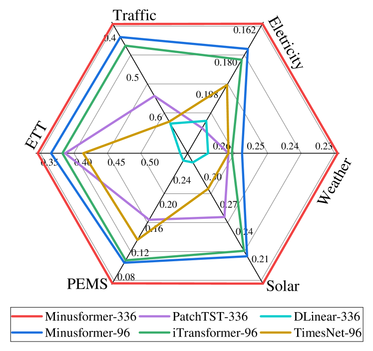
Figure 1: Comparison of the proposed Minusformer and other latest advanced models. The results (MSE) are averaged across all prediction lengths. The numerical suffix after the model indicates the input length of the model. Minusformer is configured with two versions of input length in order to align with other models.

Recently, deep learning are introduced for TS forecasting due to its powerful nonlinear fitting capabilities (Hornik, 1991), including Attention-based long-term forecasting (Zhou et al., 2021; Nie et al., 2022; Liu et al., 2023) or Graph Neural Networks (GNNs) based forecasting methods (Li et al., 2018; Wu et al., 2019). However, the latest studies suggest that the improvements in predictive performance using Attention-based methods, compared to Multi-Layer Perceptrons (MLP), have not been significant (Zeng et al., 2023; Liang et al., 2023). And their inference speed has slowed down relative to the vanilla Transformer (Liang et al., 2023). In addition, GNN-based methods have not shown substantial improvement in predictive performance compared to MLP (Shao et al., 2022).

Inspired by previous works, we found that prevalent deep models are prone to severely overfitting in the attribute dimension of TS data. As shown in Fig. 2, overfitting occurs early during training (validation loss increases significantly), even though the training loss is still declining sharply (orange line). Reorienting the aggregation direction to the temporal dimension may initially yield higher training and validation errors. Nevertheless, as the number of training batches increases, the final validation performance will show a significant improvement (olive line). If the learning process in the two directions can be better balanced, better verification performance can be achieved (violet line).

Therefore, in this paper, we delve into a de-redundancy approach that implicitly decomposes the supervision signals to progressively steer the learning process to cope with the overfitting problem. Concretely, we renovate the vanilla Transformer architecture by modifying the information aggregation mechanism, replacing addition with subtraction. Subsequently, we incorporate an auxiliary output stream into each block of the original model, thus constructing a highway that guides towards the final prediction. The output of subsequent modules in this stream will subtract the previously learned results, facilitating the model to progressively learn the residuals of the supervision signal, layer by layer. The incorporation of a dual data stems design promotes the learning-driven implicit progressive decomposition of both the input and output streams, thereby empowering the model with enhanced versatility, interpretability, and resilience against overfitting. Since all aggregations in the model consist exclusively of minus signs, it is termed a Minusformer. We validate the proposed method across a diverse range of real-world TS datasets spanning various domains. Extensive experiments demonstrate the proposed method outperform existing state-of-the-art (SOTA) methods, yielding an average performance improvement of 11.9% across various datasets. Code is available at this repository.

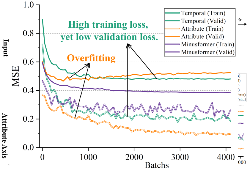
Figure 2: Generalization of the model when time series are aggregated in different directions. The experiment was conducted utilizing Transformer with 4 blocks (baseline) on the Traffic dataset.

2 Related Work

2.1 Classical Models for TS Forecasting

TS forecasting is a classic research field where numerous methods have been invented to utilize historical series to predict future missing values. Early classical methods (Piccolo, 1990; Gardner Jr, 1985; Li et al., 2010) are widely applied because of their well-defined theoretical guarantee and interpretability. For example, ARIMA (Piccolo, 1990) initially transforms a non-stationary TS into a stationary one via difference, and subsequently approximates it using a linear model with several parameters. Exponential smoothing (Gardner Jr, 1985) predicts outcomes at future horizons by computing a weighted average across historical data. In addition, some regression-based methods, e.g., random forest regression (RFR) (Liaw et al., 2002) and support vector regression (SVR) (Castro-Neto et al., 2009), etc., are also applied to TS forecasting. These methods are straightforward and have fewer parameters to tune, making them a reliable workhorse for TS forecasting. However, their shortcoming is insufficient data fitting ability, especially for high-dimensional series, resulting in limited performance.

2.2 Deep Models for TS Forecasting

The advancement of deep learning has greatly boosted the progress of TS forecasting. Specifically, convolutional neural networks (CNNs) (LeCun et al., 1998) and recurrent neural networks (RNNs) (Connor et al., 1994) have been adopted by many works to model nonlinear dependencies of TS, e.g., LSTNet (Lai et al., 2018) improve CNNs by adding recursive skip connections to capture long- and short-term temporal patterns; DeepAR (Salinas et al., 2020) predicts the probability distribution by combining autoregressive methods and RNNs. Several works have improved the series aggregation forms of Attention mechanism, such as operations of exponential intervals adopted in LogTrans (Li et al., 2019), ProbSparse activations in Informer (Zhou et al., 2021), and frequency sampling in FEDformer (Zhou et al., 2022). Besides, GNNs and TCNs have been utilized in some methods (Wu et al., 2019; Li et al., 2023; Yao et al., 2021; Liu et al., 2022a; Wu et al., 2022a) for TS forecasting on graph data. The aforementioned methods solely concentrate on the forms of aggregating input series, overlooking the challenges posed by the overfitting problem.

2.3 Decomposition for TS Forecasting

Time series exhibit a variety of patterns, and it is meaningful and beneficial to decompose them into several components, each representing an underlying category of patterns that evolving over time (Anderson, 1976). Several methods, e.g., STL (Cleveland et al., 1990), Prophet (Taylor & Letham, 2018) and N-BEATS (Oreshkin et al., 2019), commonly utilize decomposition as a preprocessing phase on historical series. There are also some methods, e.g., Autoformer (Wu et al., 2021), FEDformer (Zhou et al., 2022) and Non-stationary Transformers (Liu et al., 2022b), that harness decomposition into the Attention module. The aforementioned methods attempt to apply decomposition to input series to enhance predictability, reduce computational complexity, or ameliorate the adverse effects of non-stationarity. Nevertheless, these prevalent methods are susceptible to significant overfitting when applied to non-stationary TS. In this paper, the proposed method utilizes a progressive approach to guide the learning of each time-varying pattern. This is achieved by implicitly decomposing the supervision signals, which helps address the issue of overfitting.

3 Method

3.1 Preliminaries

The purpose of TS forecasting is to use the observed value of $I$ historical moments to predict the missing value of $O$ future moments, which can be denoted as Input-$I$-Predict-$O$. If the feature dimension of the series is denoted as $D$, its input data can be denoted as $X^{t}=\{s_{1}^{t},\cdots,s_{I}^{t}|s_{i}^{t}\in\mathcal{R}^{D}\}$, and its output can be denoted as $Y^{t}=\{s_{I+1}^{t},\cdots,s_{I+O}^{t}|s_{I+o}^{t}\in\mathcal{R}^{D}\}$, where $s_{i}^{t}$ is a subseries with dimension $d$ at the $t$-th moment. Then, we can predict $Y^{t}$ by designing a model $\mathcal{F}$ given an input $X^{t}$, which can be expressed as: $Y^{t}=\mathcal{F}(X^{t})$. Therefore, it is crucial to choose an appropriate $\mathcal{F}$ to improve the performance of the model. For denotation simplicity, the superscript $t$ will be omitted if it does not cause ambiguity in the context.

3.2 Minusformer

As shown in Fig. 3, Minusformer comprises two primary data streams. One is the input stream decomposed through multiple residual blocks with subtraction operations, while the other is the output stream that progressively learning the residuals of the supervised signals. Along the way, they pass through multiple neural blocks capable of extracting and converting signals. The base architecture is simple and versatile, yet powerful and interpretable. We now delve into how these properties are incorporated into the proposed architecture. Detailed pseudocode implementation is provided in Appendix E.

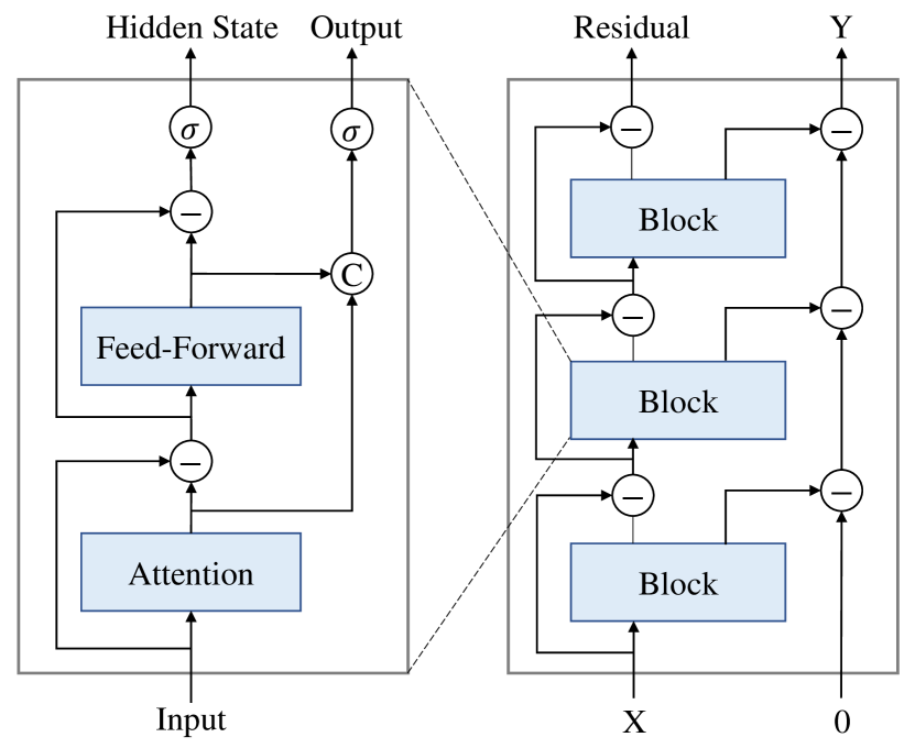
Figure 3: The framework of Minusformer.

Input: The input $X\in\mathcal{R}^{I\times D}$ is historical data of length $I$ from the current time point $t$. It is embedded before passing through the first neural block. In contrast to earlier works (Zhou et al., 2021; Wu et al., 2021; Zhou et al., 2022), we embed the temporal aspect of the input instead of the attribute aspect, which stems from our observation that directly learning attributes tends to result in significant overfitting, as aforementioned in Section 1. Here, we adopt a straightforward linear transformation to embed the input along with its temporal variates, which can be expressed as

$$X_{1} =\text{Linear}(X_{0}^{T},t),$$ (1)

where the superscript represents the number of layers of the neural networks. By utilizing the embedding layer, we obtain a unified representation of the inputs.

Backbone: The fundamental building backbone features a fork architecture, which accepts one input $X_{l}$ and produces two distinct streams, $R_{l}$ and $O_{l}$. Concretely, $R_{l}$ is the remaining portion of $X_{l}$ after it has undergone processing within a neural module, which can be expressed as

$$\hat{X}_{l} =\text{Block}(X_{l}),$$ (2a)

$$R_{l} =X_{l}-\hat{X}_{l},$$ (2b)

Equation 2 represents an implicit decomposition of $X$, which differs from the moving average adopted by (Wu et al., 2021; Zhou et al., 2022) and (Liang et al., 2023) but is similar to (Oreshkin et al., 2019). The residual information $R_{l}$ captures what remains unaltered or unprocessed, providing a basis for comparison with the transformed portion.

In the subsequent steps, our intention is to maximize the utilization of the subtracted portion $\hat{X}_{l}$. First, $\hat{X}_{l}$ is projected into the same dimension as the label that is anticipated, $Y$. This process can be expressed as

$$O_{l} =\text{Linear}(\hat{X}_{l}),$$ (3)

where $O_{l}$ is the prediction results of the $l$-th predictor. Then, $O_{l}$ will be subtracted from the outputs of the next predictor sequentially until the final predictions $Y$ is achieved. This iterative subtraction process is crucial because it facilitates the model in refining its understanding incrementally, with the objective of converging towards more accurate predictions as the layers go deeper.

Block: The basic block can be constructed utilizing widely-used neural structures, such as fully connected, convolutional, and attention layers. It is crucial to consider the characteristics of multivariate TS forecasting when selecting these fundamental neural units. We discovered that learning the feature aspect of time series results in significant overfitting, as shown in Fig. 2. Nevertheless, exclusively focusing on learning the temporal aspect of the TS will hinder the capacity of the model to capture nuanced patterns and relationships within the attributes. A ready-made solution is to utilize Attention mechanisms to learn subtle relationships between attributes. Thanks to the intrinsic sparsity of softmax activation, the model can incorporate potential attribute patterns without succumbing to overfitting.

The drawback of using Attention is that it becomes ineffective or even worsens predictive performance when various attributes are independent of each other. To mitigate this limitation, we implement a corrective measure by subtracting the Attention output from the input. This ensures that Attention can effectively capitalize on its inherent advantages, enhancing overall performance. This process can be expressed as

$$\hat{X}_{l,1} =\text{Attention}(X_{l,1}),$$ (4a)

$$R_{l,1} =X_{l,1}-\delta\hat{X}_{l,1}.$$ (4b)

where $\delta$ is the Dirac function. $\delta$ serves to eliminate the Attention layer when it exerts adverse effects, thereby enabling the unimpeded flow of input towards the feedforward layers. Similarly, the input signal processed by the feedforward layer will also be subtracted from the input, which can be expressed as

$$\hat{X}_{l,2} =\text{FeedForward}(R_{l,1}),$$ (5a)

$$R_{l,2} =X_{l,2}-\hat{X}_{l,2}.$$ (5b)

The feedforward layer consists of two identity mappings inserted with an activation function, exclusively performs nonlinear transformations on the temporal aspect. This holds particular crucial for multivariate characterized by a strong independence among their attributes.

Presently, within the entire block, there are two streams: one consists of the outputs $\hat{X}_{l}$ transformed by the neural modules, and the other encompasses the residuals $R_{l}$ obtained by subtracting $\hat{X}_{l}$ from the input. Upon passing through a gate mechanism, they are directed toward the next block or projected into the output space.

Gate: Drawing inspiration from RNNs, our aspiration is for each neural module to autonomously regulate the pace of information transmission, akin to the inherent control exhibited by cells in RNNs. Therefore, we introduced a gate mechanism at the conclusion of each block for both streams. For residual stream, its gate mechanism can be expressed as

$$X_{l+1} =\sigma(\theta_{1}(R_{l,2}))\cdot\theta_{2}(R_{l,2}),$$ (6)

where $\sigma$ is the sigmoid function, $\theta_{1}$ and $\theta_{2}$ are learnable neurons with different parameters. Likewise, for the intermediate output $\hat{X}_{l}$, the gate mechanism can be expressed as

$${O}_{l+1} =\sigma(\theta_{3}([\hat{X}_{l,1},\hat{X}_{l,2}]))\cdot\theta_{4}([\hat{X}_{l,1},\hat{X}_{l,2}]),$$ (7)

where the square brackets ‘[ ]’ indicate concatenation operation. Equation 7 facilitates the comprehensive utilization of outputs from both the Attention and feedforward layers. The gating mechanism has the capacity to induce signal morphing on both streams, effectively scaling the quantity of information output from the current block. It enables the model to discerningly amplify or attenuate the influence of specific stages, thereby fully leveraging the profound structure of Minusformer to enhance its modeling prowess.

Minus: The primary distinctive characteristic of Minusformer lies in the exclusive utilization of subtraction for all skip connections throughout the entire architecture. Below, we will delineate their respective functions for residual streams $R_{l}$ and output streams $O_{l}$.

Table 1: Multivariate TS forecasting results on six benchmark datasets.

Model		Minusformer-336			Minusformer-96			iTransformer-96		PatchTST-336		Crossformer-720♢		SCINet-168		TimesNet-96		DLinear-336		FEDformer-96		Autoformer-96		Informer-96
	Length	MSE	MAE	IMP	MSE	MAE	IMP	MSE	MAE	MSE	MAE	MSE	MAE	MSE	MAE	MSE	MAE	MSE	MAE	MSE	MAE	MSE	MAE	MSE	MAE
ETT	96	0.280	0.336	4.72%	0.289	0.340	2.64%	0.297	0.349	0.302	0.348	0.745	0.584	0.707	0.621	0.340	0.374	0.333	0.387	0.358	0.397	0.346	0.388	3.755	1.525
	192	0.332	0.371	9.94%	0.349	0.374	7.33%	0.380	0.400	0.388	0.400	0.877	0.656	0.860	0.689	0.402	0.414	0.477	0.476	0.429	0.439	0.456	0.452	5.602	1.931
	336	0.362	0.392	12.34%	0.393	0.405	7.21%	0.428	0.432	0.426	0.433	1.043	0.731	1.000	0.744	0.452	0.452	0.594	0.541	0.496	0.487	0.482	0.486	4.721	1.835
	720	0.410	0.429	3.79%	0.433	0.435	0.42%	0.427	0.445	0.431	0.446	1.104	0.763	1.249	0.838	0.462	0.468	0.831	0.657	0.463	0.474	0.515	0.511	3.647	1.625
	Avg	0.346	0.382	7.90%	0.366	0.388	4.55%	0.383	0.407	0.387	0.407	0.942	0.684	0.954	0.723	0.414	0.427	0.559	0.515	0.437	0.449	0.450	0.459	4.431	1.729
Traffic	96	0.350	0.250	9.05%	0.386	0.258	3.00%	0.395	0.268	0.544	0.359	0.522	0.290	0.788	0.499	0.593	0.321	0.650	0.396	0.587	0.366	0.613	0.388	0.719	0.391
	192	0.375	0.261	7.75%	0.398	0.263	4.63%	0.417	0.276	0.540	0.354	0.530	0.293	0.789	0.505	0.617	0.336	0.598	0.370	0.604	0.373	0.616	0.382	0.696	0.379
	336	0.381	0.264	9.36%	0.409	0.270	5.07%	0.433	0.283	0.551	0.358	0.558	0.305	0.797	0.508	0.629	0.336	0.605	0.373	0.621	0.383	0.622	0.337	0.777	0.420
	720	0.386	0.268	14.30%	0.431	0.287	6.34%	0.467	0.302	0.586	0.375	0.589	0.328	0.841	0.523	0.640	0.350	0.645	0.394	0.626	0.382	0.660	0.408	0.864	0.472
	Avg	0.373	0.261	10.15%	0.406	0.270	4.79%	0.428	0.282	0.555	0.362	0.550	0.304	0.804	0.509	0.620	0.336	0.625	0.383	0.610	0.376	0.628	0.379	0.764	0.416
Electricity	96	0.128	0.223	10.30%	0.143	0.235	2.73%	0.148	0.240	0.195	0.285	0.219	0.314	0.247	0.345	0.168	0.272	0.197	0.282	0.193	0.308	0.201	0.317	0.274	0.368
	192	0.148	0.24	6.89%	0.162	0.253	0.00%	0.162	0.253	0.199	0.289	0.231	0.322	0.257	0.355	0.184	0.289	0.196	0.285	0.201	0.315	0.222	0.334	0.296	0.386
	336	0.164	0.26	5.61%	0.179	0.271	-0.65%	0.178	0.269	0.215	0.305	0.246	0.337	0.269	0.369	0.198	0.300	0.209	0.301	0.214	0.329	0.231	0.338	0.300	0.394
	720	0.192	0.284	12.54%	0.204	0.294	8.29%	0.225	0.317	0.256	0.337	0.280	0.363	0.299	0.390	0.220	0.320	0.245	0.333	0.246	0.355	0.254	0.361	0.373	0.439
	Avg	0.158	0.252	8.95%	0.172	0.263	2.94%	0.178	0.270	0.216	0.304	0.244	0.334	0.268	0.365	0.192	0.295	0.212	0.300	0.214	0.327	0.227	0.338	0.311	0.397
Weather	96	0.150	0.201	9.93%	0.169	0.209	2.61%	0.174	0.214	0.177	0.218	0.158	0.230	0.221	0.306	0.172	0.220	0.196	0.255	0.217	0.296	0.266	0.336	0.300	0.384
	192	0.194	0.244	8.08%	0.220	0.254	0.23%	0.221	0.254	0.225	0.259	0.206	0.277	0.261	0.340	0.219	0.261	0.237	0.296	0.276	0.336	0.307	0.367	0.598	0.544
	336	0.245	0.282	8.30%	0.276	0.296	0.36%	0.278	0.296	0.278	0.297	0.272	0.335	0.309	0.378	0.280	0.306	0.283	0.335	0.339	0.380	0.359	0.395	0.578	0.523
	720	0.320	0.336	7.17%	0.354	0.346	0.99%	0.358	0.349	0.354	0.348	0.398	0.418	0.377	0.427	0.365	0.359	0.345	0.381	0.403	0.428	0.419	0.428	1.059	0.741
	Avg	0.227	0.266	8.85%	0.255	0.276	1.66%	0.258	0.279	0.259	0.281	0.259	0.315	0.292	0.363	0.259	0.287	0.265	0.317	0.309	0.360	0.338	0.382	0.634	0.548
Solar	96	0.181	0.222	8.58%	0.192	0.222	5.87%	0.203	0.237	0.234	0.286	0.310	0.331	0.237	0.344	0.250	0.292	0.290	0.378	0.242	0.342	0.884	0.711	0.236	0.259
	192	0.198	0.239	11.73%	0.230	0.251	2.56%	0.233	0.261	0.267	0.310	0.734	0.725	0.280	0.380	0.296	0.318	0.320	0.398	0.285	0.380	0.834	0.692	0.217	0.269
	336	0.202	0.245	14.40%	0.243	0.263	2.84%	0.248	0.273	0.290	0.315	0.750	0.735	0.304	0.389	0.319	0.330	0.353	0.415	0.282	0.376	0.941	0.723	0.249	0.283
	720	0.206	0.252	12.82%	0.243	0.265	3.02%	0.249	0.275	0.289	0.317	0.769	0.765	0.308	0.388	0.338	0.337	0.356	0.413	0.357	0.427	0.882	0.717	0.241	0.317
	Avg	0.197	0.240	11.92%	0.227	0.250	3.58%	0.233	0.262	0.270	0.307	0.641	0.639	0.282	0.375	0.301	0.319	0.330	0.401	0.291	0.381	0.885	0.711	0.235	0.280
PEMS	12	0.057	0.157	14.74%	0.067	0.171	3.68%	0.071	0.174	0.099	0.216	0.090	0.203	0.066	0.172	0.085	0.192	0.122	0.243	0.126	0.251	0.272	0.385	0.126	0.233
	24	0.070	0.173	19.33%	0.093	0.203	-0.50%	0.093	0.201	0.142	0.259	0.121	0.240	0.085	0.198	0.118	0.223	0.201	0.317	0.149	0.275	0.334	0.440	0.139	0.250
	36	0.083	0.186	27.39%	0.125	0.237	-0.21%	0.125	0.236	0.211	0.319	0.202	0.317	0.127	0.238	0.155	0.260	0.333	0.425	0.227	0.348	1.032	0.782	0.186	0.289
	48	0.091	0.195	35.45%	0.151	0.262	4.29%	0.160	0.270	0.269	0.370	0.262	0.367	0.178	0.287	0.228	0.317	0.457	0.515	0.348	0.434	1.031	0.796	0.233	0.323
	Avg	0.075	0.178	26.54%	0.109	0.218	2.39%	0.113	0.221	0.180	0.291	0.169	0.281	0.114	0.224	0.147	0.248	0.278	0.375	0.213	0.327	0.667	0.601	0.171	0.274
$1^{st}$ or $2^{st}$ Count		30	30	30	19	27	27	3	2	0	0	3	0	2	1	0	0	1	0	0	0	0	0	2	0

• IMP refers to the average performance improvement compared to the latest iTransformer with the best average performance. ${\diamondsuit}$ denotes the maximum search range of the input length.

For residual streams, it transforms the input into a procedural form through parametric decomposition. As demonstrated by Equations 4 and 5, the residuals preserve the unaltered or unprocessed signal, enabling the model to harness deep structures for progressively refinement. For output streams, it leverages information that has been meticulously refined layer by layer to systematically learn a decomposition of the outputs. Throughout this progression, the label $Y$ is treated as a residual, which can be expressed as

$$Y =i\sum_{l=0}^{\lfloor\frac{L}{2}\rfloor}O_{2l+1}-i\sum_{l=0}^{\lfloor\frac{L}{2}\rfloor}O_{2l},$$ (8)

where $i=1$ if $L\bmod 2=1$, else $i=-1$. Opting to directly treat $Y$ as a residual term, as opposed to decomposing it directly, confers distinct advantages. Principally, Equation 8 more accurately encapsulates the essence of progressive learning. Indeed, with each progression into deeper layers, the model subtracts the results previously learned. Secondly, the process of layer-by-layer subtraction empowers the model to comprehend the overarching envelope and complementary components of the series progressively, transitioning from a broad overview to finer details. Lastly, the interpretability of the output from each layer in Minusformer is evident, as the decomposition process of $Y$ is encapsulated within the two sequential decomposition series illustrated on the right side of Equation 8. The substantiation of the above conclusions is further elucidated through the visual representation of the output from each layer in Minusformer, as expounded in Section 4.5.

Table 2: Univariate TS forecasting results on five benchmark datasets.

Model	Minusformer-96		Periodformer-144♢		FEDformer-96		Autoformer-96		Informer-96		LogTrans-96		Reformer-96
Metric	MSE	MAE	MSE	MAE	MSE	MAE	MSE	MAE	MSE	MAE	MSE	MAE	MSE	MAE
ETTh1	0.072	0.206	0.093	0.237	0.111	0.257	0.105	0.252	0.199	0.377	0.345	0.513	0.624	0.600
ETTh2	0.185	0.337	0.192	0.343	0.206	0.350	0.218	0.364	0.243	0.400	0.252	0.408	3.472	1.283
ETTm1	0.052	0.172	0.059	0.201	0.069	0.202	0.081	0.221	0.281	0.441	0.231	0.382	0.523	0.536
ETTm2	0.118	0.254	0.115	0.253	0.135	0.278	0.130	0.271	0.147	0.293	0.130	0.277	0.136	0.288
Traffic	0.132	0.212	0.150	0.233	0.177	0.270	0.261	0.365	0.309	0.388	0.341	0.417	0.375	0.434
Electricity	0.314	0.401	0.298	0.389	0.347	0.434	0.414	0.479	0.372	0.444	0.410	0.473	0.352	0.435
Weather	0.0015	0.0293	0.0017	0.0317	0.008	0.067	0.0083	0.0700	0.0033	0.0438	0.0059	0.0563	0.0115	0.0785
Exchange	0.429	0.453	0.353	0.434	0.499	0.512	0.578	0.537	1.511	1.029	1.350	0.810	1.028	0.812
$1^{\text{st}}$ Count	24	27	14	12	0	1	0	0	0	0	2	0	0	0

• All results are averaged across all prediction lengths. The results for all prediction lengths are provided in Appendix G. ${\diamondsuit}$ denotes the maximum search range of the input length.

4 Experiments

Minusformer undergoes a comprehensive evaluation across the widely employed real-world datasets, including multiple mainstream TS forecasting applications such as energy, traffic, electricity, weather, transportation and exchange.

Implementation Details: The model undergoes training utilizing the ADAM optimizer (Kingma & Ba, 2015) and minimizing the Mean Squared Error (MSE) loss function. The training process is halted prematurely, typically within 10 epochs. The Minusformer architecture solely comprises the embedding layer and backbone architecture, devoid of any additional introduced hyperparameters. Refer to Appendix B for the hyperparameter sensitivity analysis. During model validation, two evaluation metrics are employed: MSE and Mean Absolute Error (MAE). Given the potential competitive relationship between the two indicators, MSE and MAE, we use the average of the two ($\frac{MSE+MAE}{2}$) to evaluate the overall performance of the model.

Baselines: Given the comparatively subpar performance of traditional models like ARIMA, as demonstrated in (Zhou et al., 2021; Wu et al., 2021), our main approach for comparisons is to adopt SOTA methods. For comparison purposes, 12 SOTA Transformer-based models are adopted as baselines, including iTransformer (Liu et al., 2023), PatchTST (Nie et al., 2022), Crossformer (Zhang & Yan, 2022), SCINet (Liu et al., 2022a), TimesNet (Wu et al., 2022a), DLinear (Zeng et al., 2023), Periodformer (Liang et al., 2023), FEDformer (Zhou et al., 2022), Autoformer (Wu et al., 2021), Informer (Zhou et al., 2021), LogTrans (Li et al., 2019) and Reformer (Kitaev et al., 2020). The numerical suffix attached to each model represents the input length utilized by the respective model.

4.1 Experimental Results

All datasets are adopted for both multivariate (multivariate predict multivariate) and univariate (univariate predicts univariate) tasks. The detailed information pertaining to the datasets can be located in Appendix A. The models used in the experiments are evaluated over a wide range of prediction lengths to compare performance on different future horizons: 96, 192, 336 and 720. The experimental settings are the same for both multivariate and univariate tasks. Please refer to Appendix D for more experiments on the full ETT dataset.

Multivariate Results: The results for multivariate TS forecasting are outlined in Table 1, with the optimal results highlighted in red and the second-best results emphasized with underlined. Due to variations in input lengths among different methods, for instance, PatchTST and DLinear employing an input length of 336, while Crossformer and Periodformer search for the input length without surpassing the maximum setting (720 in Crossformer, 144 in Periodformer), we have configured two versions of the proposed Minusformer, each with different input lengths (96 and 336), for performance evaluation.

As shown in Table 1, the proposed Minusformer achieves the consistent SOTA performance across all datasets and prediction length configurations. iTransformer and PatchTST stand out as the latest models acknowledged for their exceptional average performance. Compared with them, the proposed Minusformer-336 demonstrates an average performance reduction of 11.9% and 20.6%, respectively, achieving a substantial performance improvement. Next, our primary focus shifts to analyzing the performance gains of Minusformer-96. Minusformer-96 demonstrates an average performance reduction of 3.0% and 13.4%, respectively. It achieves advanced performance, averaging 23 items across six datasets, with an improvement (IMP) in average performance on each dataset. For example, when compared to iTransformer and PatchTST under the input-96-predict-720 setting, Minusformer achieves a 7.7% (0.467$\rightarrow$0.431) and 26.5% (0.586$\rightarrow$0.431) in MSE reduction for Traffic, and 9.3% (0.225$\rightarrow$0.204) and 20.3% (0.256$\rightarrow$0.204) in Electricity, etc. The experimental results presented above confirm that the proposed Minusformer demonstrates superior prediction performance across different datasets with varying horizons. This suggests its efficacy in handling multivariate time series forecasting tasks.

Univariate Results: The average results for univariate TS forecasting are shown in Table 2. It is evident that the proposed Minusformer continues to maintain a SOTA performance across various prediction length settings compared to the benchmarks. In summary, compared with the hyperparameter-searched Periodformer, Minusformer yields an average 4.8% reduction across five datasets, and it achieves an average of 26 best terms. Specifically, under the input-96-predict-96 setting, Minusformer yields a reduction of 11.2% (0.143$\rightarrow$0.127) in MSE for Traffic. Additionally, under the input-96-predict-720 setting, Minusformer gives 7.9% (0.152$\rightarrow$0.140) MSE reduction in ETT, and 17.7% (0.164$\rightarrow$0.135) MSE reduction in Traffic. Obviously, the experimental results again verify the superiority of Minusformer on univariate TS forecasting tasks.

4.2 Comparative Analysis

Notably, several pioneering models have also achieved competitive performance on certain datasets under particular settings. For instance, Informer, considered a groundbreaking model in long-term TS forecasting, demonstrates advanced performance on the Solar-Energy dataset with input-96-predict-192 and -720 settings. This is due to the substantial presence of zero values on each column attribute of the Solor-Energy dataset. This renders the KL-divergence based ProbSparse Attention, as adopted in Informer, highly effective on this sparse dataset. Additionally, linear-based methods (e.g., DLinear) have demonstrated promising results on the Weather dataset with input-336-predict-720 setting, while convolution-based methods (e.g., SCINet) have yielded favorable results on the PEMS dataset with input-168-predict-192 setting. This phenomenon can be ascribed to a twofold interplay of factors. Previously, the diversity of input settings exerts a direct influence on model generalization. Secondarily, other models exhibit a propensity to overfit non-stationary TS characterized by aperiodic fluctuations. Remarkably, Minusformer adeptly mitigates both overfitting and underfitting challenges in multivariate TS forecasting, thereby enhancing its overall performance. Particularly on datasets with numerous attributes, e.g., Traffic and Solor-Energy, Minusformer achieves superior performance by feeding the learned meaningful patterns to the output layer at each block.

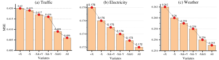
Figure 4: Ablation studies on various components of Minusformer. All results are averaged across all prediction lengths. The variables $X$ and $Y$ represent the input and output streams, while the signs ‘+’ and ‘-’ denote the addition or subtraction operations used when the streams’ aggregation. The letter ‘G’ denotes adding a gating mechanism to the output of each block.

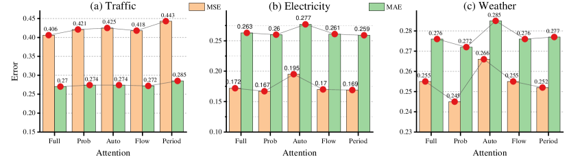
Figure 5: Ablation studies of Minusformer using various Attention. All results are averaged across all prediction lengths. The tick labels of the X-axis are the abbreviation of Attention types. The detailed setup and results for all prediction lengths are provided in Appendix C.

4.3 Effectiveness

To validate the effectiveness of Minusformer components, we conduct comprehensive ablation studies encompassing both component replacement and component removal experiments, as shown in Fig. 4. We utilize signs ‘+’ and ‘-’ to denote the utilization of addition or subtraction operations during the aggregation process of the input or output streams. In cases involving only input streams, it becomes evident that the model’s average performance is superior when employing subtraction (-X) compared to when employing addition (+X). E.g., on the Electricity dataset, forecast error is reduced by 1.1% (0.178$\rightarrow$0.176). Moreover, with the introduction of a high-speed output stream to the model, shifting the aggregation method of the output stream from addition (+Y) to subtraction (-Y) is poised to further enhance the model’s performance. Afterward, incorporating gating mechanisms (G) into the model holds the potential to improve predictive performance again. E.g., on the Traffic dataset, forecast error is reduced by 2.4% (0.419$\rightarrow$0.409). In summary, integrating the advantages of the aforementioned components has the potential to significantly boost the model’s performance across the board.

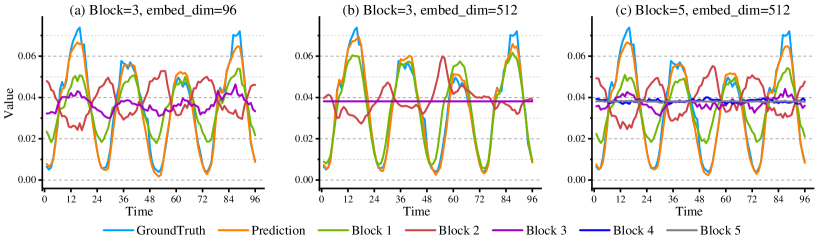
Figure 6: Visualization depicting the output of each block in Minusformer. The experiment was implemented on the Traffic dataset using the setting of Input-96-Predict-96. The utilized models have the same hyperparameter settings and similar performance.

4.4 Generality

To investigate Minusformer’s generality as a universal architecture, we substituted its original Attention with other novel Attention mechanisms to observe the resulting changes in model performance. As shown in Fig. 5, after harnessing the newly invented Attention within Minusformer, its performance exhibited considerable variation. E.g., the average MSE of Prob-Attention (Zhou et al., 2021) on the Electricity and Weather datasets witnessed a reduction of 46% (0.311$\rightarrow$0.167) and 61% (0.634$\rightarrow$0.245), respectively, surpassing Full-Attention and achieving new SOTA performance. Furthermore, both Period-Attention (Liang et al., 2023) and Flow-Attention (Wu et al., 2022b) demonstrate commendable performance on the aforementioned datasets. The improvement in Auto-Correlation (Wu et al., 2021) falls short of expectations, primarily due to the incapacity of its autocorrelation mechanism to capture nuanced patterns of change within attributes characterized by substantial fluctuations. The conducted experiments suggest that Minusformer can serve as a versatile architecture, amenable to the integration of novel modules, thereby facilitating the enhancement of performance in the domain of TS forecasting.

4.5 Interpretability

The intrinsic characteristic of Minusformer lies in the alignment of the output from each block with the shape of the final output. This alignment, in turn, expedites the decomposition and visualization of the model’s learning process. As depicted in Fig. 6, the output of each block in the Minusformer is visualized, with variations in both width and depth configurations. Moreover, Attention within each block is visualized in Fig. 7, which corresponds to the model in Fig. 6(a). It becomes evident that each block discerns and assimilates meaningful patterns within the series. Specifically, comparing Fig. 6(a) and 6(b), when the embedding dimension is low, each block must learn salient patterns. However, as the model capacity increases, the efficacy of the deep blocks diminishes. E.g., block 3 in Fig. 6(b) solely acquires knowledge of a single constant. Further, increasing the depth of the model, as depicted in Fig. 6(c), it becomes evident that the amplitude of the shallow block decreases, and numerous components are transferred to the deep block. E.g., block 3 in Fig. 6(c) exhibits the same behavior as in Fig. 6(a). This suggests that increasing the depth of Minusformer enhances its learning capacity without heightening the risk of overfitting.

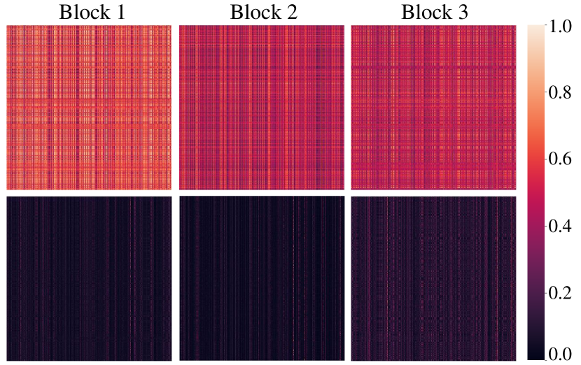
Figure 7: Visualization of Attention scores (top) and post-softmax scores (bottom) in each block. The results are averaged across all heads. The detailed results are provided in Appendix F.

4.6 Go Deeper

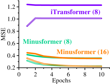
Figure 8: Process of training (Dash) and validation (Solid) when models go deeper.

Given the Minusformer’s robustness against overfitting, it can be designed with considerable depth. Fig. 8 illustrates the scenarios when models go deeper. Serious overfitting happens when the number of iTransformer blocks is increased from 4 to 8. However, even with the Minusformer blocks deepened to 8 or 16, it continues to exhibit excellent performance. Additionally, Minusformer is less sensitive to hyperparameters, with details presented in Appendix B.

5 Conclusion

In this paper, we designed a architecture utilizing exclusively minus signs for information aggregation, specifically crafted to address the ubiquitous overfitting problem prevalent in TS forecasting models, which is called Minusformer. Minusformer comprising two distinct data streams. One stream involves the input, which undergoes implicit decomposition via multiple residual blocks with subtraction operations. The other stream pertains to the output, wherein the model progressively learns the residuals of the supervised signals, layer by layer. The designed architecture facilitates the learning-driven, implicit, progressive decomposition of both the input and output streams, thereby empowering the model with enhanced generality, interpretability, and resilience against overfitting. Minusformer is insensitive to hyperparameters and can be designed very deep without overfitting. Extensive experiments demonstrate that Minusformer achieves SOTA performance.

Impact Statements

This paper presents work whose goal is to advance the field of Time Series Forecasting. There are many potential societal consequences of our work, none which we feel must be specifically highlighted here.

Appendix A Dataset

The information of the experiment datasets used in this paper are summarized as follows: (1) Electricity Transformer Temperature (ETT) dataset (Zhou et al., 2021), which contains the data collected from two electricity transformers in two separated counties in China, including the load and the oil temperature recorded every 15 minutes (ETTm) or 1 hour (ETTh) between July 2016 and July 2018. (2) Electricity (ECL) dataset collects the hourly electricity consumption of 321 clients (each column) from 2012 to 2014. (3) Exchange (Lai et al., 2018) records the current exchange of 8 different countries from 1990 to 2016. (4) Traffic dataset records the occupation rate of freeway system across State of California measured by 861 sensors. (5) Weather dataset records every 10 minutes for 21 meteorological indicators in Germany throughout 2020. (6) Solar-Energy (Lai et al., 2018) documents the solar power generation of 137 photovoltaic (PV) facilities in the year 2006, with data collected at 10-minute intervals. (7) The PEMS dataset (Liu et al., 2022a) comprises publicly available traffic network data from California, collected within 5-minute intervals and encompassing 358 attributes. The detailed statistics information of the datasets is shown in Table 3.

Table 3: Details of the seven TS datasets.

Dataset	length	features	frequency
ETTh1	17,420	7	1h
ETTh2	17,420	7	1h
ETTm1	69,680	7	15m
ETTm2	69,680	7	15m
Electricity	26,304	321	1h
Exchange	7,588	8	1d
Traffic	17,544	862	1h
Weather	52,696	21	10m
Solar	52,560	137	10m
PEMS	26,208	358	5m

• The letters $m$, $h$, and $d$ represent minutes, hours, and days, respectively.

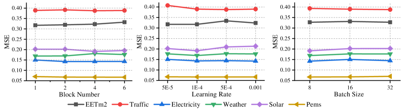
Figure 9: Hyperparameter sensitivity with respect to the number of block, the learning rate and the number of batch size. The results are recorded with the input length $I=96$ and the prediction length $O=12$ for PEMS and $O=96$ for others.

Appendix B Hyperparameter Sensitivity

We evaluate the hyperparameter sensitivity of Minusformer with respect to the learning rate, the number of the block and the batch size. As shown in Fig. 9, the performance of Minusforemr fluctuates under different hyperparameter settings. In most cases, augmenting the quantity of blocks tends to enhance model performance. Once again, this confirms that Minusformer exhibits resilience against overfitting across diverse datasets. Notably, we observe that the learning rate, being the most prevalent influencing factor, especially in scenarios involving numerous attributes. In addition, modifying the batch size induces minor fluctuations in the model’s performance, albeit with a limited impact. In summary, Minusformer exhibits low sensitivity to these hyperparameters, thereby enhancing its resilience against overfitting.

Appendix C Different Attention Promotion

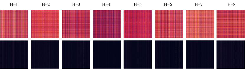
Figure 10: Visualization of Attention utilized in Minusformer. The model is trained on Traffic dataset with 862 attributes under the setting of Input-96-Predict-96. Both the Attention score (top) and the post-softmax score (below) of the 8 heads (H) are from the first block.

We visualized the Attention maps for all Attention heads in the initial layer of Minusformer, and the results are presented in Fig. 10. It is evident that the Attention score graph exhibits numerous bar structures, which is especially prominent on the post-softmax Attention map. This implies that there exists a row in Query that bears a striking resemblance to all the columns in Key. This scenario arises when there are numerous attributes, many of which are homogeneously represented. Our speculation suggests that this capability of the Attention may explain its ability to capture subtle patterns in TS without succumbing to overfitting. Furthermore, we substituted its original Attention with other novel Attention mechanisms to compare the resulting changes in model performance. The full results for all prediction lengths are provided in Table 4.

Table 4: Ablation of different Attention layers.

Attention Layer		FullAttention		ProbAttention		AutoCorrelation		FlowAttention		PeriodAttention
Dataset	Length	MSE	MAE	MSE	MAE	MSE	MAE	MSE	MAE	MSE	MAE
Traffic	96	0.386	0.258	0.390	0.259	0.396	0.261	0.385	0.256	0.414	0.273
	192	0.398	0.263	0.410	0.268	0.413	0.268	0.406	0.265	0.431	0.279
	336	0.409	0.270	0.425	0.274	0.429	0.275	0.424	0.274	0.447	0.286
	720	0.431	0.287	0.459	0.293	0.461	0.293	0.459	0.293	0.478	0.303
	Avg	0.406	0.270	0.421	0.274	0.425	0.274	0.418	0.272	0.443	0.285
Electricity	96	0.143	0.235	0.136	0.229	0.174	0.256	0.141	0.233	0.142	0.233
	192	0.162	0.253	0.154	0.246	0.179	0.263	0.160	0.251	0.157	0.247
	336	0.179	0.271	0.172	0.268	0.195	0.279	0.175	0.267	0.172	0.264
	720	0.204	0.294	0.205	0.298	0.232	0.311	0.203	0.294	0.204	0.293
	Avg	0.172	0.263	0.167	0.260	0.195	0.277	0.170	0.261	0.169	0.259
Weather	96	0.169	0.209	0.159	0.204	0.179	0.220	0.169	0.209	0.170	0.212
	192	0.220	0.254	0.207	0.248	0.228	0.261	0.220	0.255	0.214	0.253
	336	0.276	0.296	0.265	0.291	0.288	0.304	0.276	0.294	0.273	0.296
	720	0.354	0.346	0.350	0.347	0.367	0.356	0.354	0.348	0.352	0.347
	Avg	0.255	0.276	0.245	0.273	0.266	0.285	0.255	0.276	0.252	0.277

• The input length $I$ is set as 96, while the prediction lengths $O\in$ {96, 192, 336, 720}.

Appendix D Full Results on ETT Dataset

The ETT dataset records electricity data of four different granularities and types. We offer an in-depth comparison of Minusformer utilizing the complete ETT dataset to facilitate future research endeavors. Detailed results are provided in Table 5. It is evident that Minusformer demonstrates excellent performance on the complete ETT dataset.

Table 5: Full Multivariate Forecasting Results on ETT dataset.

Models		Minusformer-96		Periodformer-144♢		FEDformer-96		Autoformer-96		Informer-96		LogTrans-96		Reformer-96
	Length	MSE	MAE	MSE	MAE	MSE	MAE	MSE	MAE	MSE	MAE	MSE	MAE	MSE	MAE
ETTh1	96	0.370	0.394	0.375	0.395	0.395	0.424	0.449	0.459	0.865	0.713	0.878	0.74	0.837	0.728
	192	0.423	0.427	0.413	0.421	0.469	0.47	0.5	0.482	1.008	0.792	1.037	0.824	0.923	0.766
	336	0.465	0.446	0.443	0.441	0.530	0.499	0.521	0.496	1.107	0.809	1.238	0.932	1.097	0.835
	720	0.465	0.464	0.467	0.469	0.598	0.544	0.514	0.512	1.181	0.865	1.135	0.852	1.257	0.889
	Avg	0.431	0.433	0.425	0.432	0.498	0.484	0.496	0.487	1.040	0.795	1.072	0.837	1.029	0.805
ETTh2	96	0.291	0.342	0.313	0.356	0.394	0.414	0.358	0.397	3.755	1.525	2.116	1.197	2.626	1.317
	192	0.371	0.391	0.389	0.405	0.439	0.445	0.456	0.452	5.602	1.931	4.315	1.635	11.12	2.979
	336	0.412	0.427	0.418	0.432	0.482	0.48	0.482	0.486	4.721	1.835	1.124	1.604	9.323	2.769
	720	0.418	0.438	0.427	0.444	0.5	0.509	0.515	0.511	3.647	1.625	3.188	1.54	3.874	1.697
	Avg	0.373	0.400	0.387	0.409	0.454	0.462	0.453	0.462	4.431	1.729	2.686	1.494	6.736	2.191
ETTm1	96	0.317	0.356	0.337	0.378	0.378	0.418	0.505	0.475	0.672	0.571	0.600	0.546	0.538	0.528
	192	0.363	0.379	0.413	0.431	0.464	0.463	0.553	0.496	0.795	0.669	0.837	0.7	0.658	0.592
	336	0.397	0.407	0.428	0.441	0.508	0.487	0.621	0.537	1.212	0.871	1.124	0.832	0.898	0.721
	720	0.454	0.442	0.483	0.483	0.561	0.515	0.671	0.561	1.166	0.823	1.153	0.82	1.102	0.841
	Avg	0.383	0.396	0.415	0.433	0.478	0.471	0.588	0.517	0.961	0.734	0.929	0.725	0.799	0.671
ETTm2	96	0.177	0.259	0.186	0.274	0.204	0.288	0.255	0.339	0.365	0.453	0.768	0.642	0.658	0.619
	192	0.239	0.299	0.252	0.317	0.316	0.363	0.281	0.34	0.533	0.563	0.989	0.757	1.078	0.827
	336	0.298	0.340	0.311	0.355	0.359	0.387	0.339	0.372	1.363	0.887	1.334	0.872	1.549	0.972
	720	0.394	0.394	0.402	0.405	0.433	0.432	0.422	0.419	3.379	1.338	3.048	1.328	2.631	1.242
	Avg	0.277	0.323	0.288	0.338	0.328	0.368	0.324	0.368	1.410	0.810	1.535	0.900	1.479	0.915
$1^{\text{st}}$ Count		17	17	3	3	0	0	0	0	0	0	2	0	0	0

• ${\diamondsuit}$ denotes the maximum search range of the input length.

Appendix E Pseudocode of Minusformer

To facilitate a comprehensive understanding of Minusformer’s working principle, we offer detailed pseudocode outlining its implementation, as shown in Algorithm 1. The implementation presented here outlines the core ideas of Minusformer. For specific code implementation, please refer to our repository. It is evident that the deployment procedure of Minusformer exhibits a relative simplicity, characterized by the inclusion of several iteratively applied blocks. This property renders it highly versatile for integrating newly devised Attention mechanisms or modules. As demonstrated in Appendix C, the substitution of Attention mechanisms in Minusformer with novel alternatives yields superior generalization.

Algorithm 1 Minusformer Architecture.

0:  Batch size $B$, input lookback time series $\mathbf{X}\in\mathbb{R}^{B\times I\times D}$; input length $I$; predicted length $O$; embedding dimension $E$; the number of the block $L$.

1:  $\mathbf{X}_{0}=\texttt{StandardScaler}(\mathbf{X}^{T})$ {$\mathbf{X}_{0}\in\mathbb{R}^{B\times D\times I}$}

2:  $\triangleright\$ Apply a linear transformation to the temporal dimension of X to align it with the embedding dimension.

3:  $\mathbf{X}_{1}=\texttt{Linear}(\mathbf{X}_{0})$   {$\mathbf{X}^{1}\in\mathbb{R}^{B\times D\times E}$}   {The embedded X enters the backbone as an input stream.}

4:  $O_{0}=0$  {Set the initial value of the output stream to 0.}

5:  $\textbf{for}\ l\ \textbf{in}\ \{1,\cdots,L\}\textbf{:}$  {Run through the backbone.}

6:  for $\triangleright\$ Apply attention to the input stream.

7:  $\textbf{{\color[rgb]{1,1,1}for}}\ \mathbf{\hat{X}}_{l,1}=\texttt{Attention}(\mathbf{X}_{l,1})$  {$\mathbf{\hat{X}}_{l,1}\in\mathbb{R}^{B\times D\times E}$}

8:  for $\triangleright\$ Subtracting the attention output from the input.

9:  $\textbf{{\color[rgb]{1,1,1}for}}\ \mathbf{R}_{l,1}=\mathbf{X}_{l,1}-\delta\ \texttt{Dropout}(\mathbf{\hat{X}}_{l,1})$  {$\mathbf{R}_{l,1}\in\mathbb{R}^{B\times D\times E}$}

10:  for $\triangleright\$ LayerNorm is adopted to reduce attributes discrepancies.

11:  $\textbf{{\color[rgb]{1,1,1}for}}\mathbf{X}_{l,2}=\mathbf{R}_{l,1}=\texttt{LayerNorm}(\mathbf{R}_{l,1})$

12:  for $\triangleright\$The feedforward exclusively performs nonlinear transformations on the temporal aspect.

13:  $\textbf{{\color[rgb]{1,1,1}for}}\ \mathbf{\hat{X}}_{l,2}=\texttt{FeedForward}(\mathbf{R}_{l,1})\big{)}$  {$\mathbf{H}^{l}\in\mathbb{R}^{B\times D\times E}$}

14:  for $\triangleright\$ Subtracting the feedforward output from the input.

15:  $\textbf{{\color[rgb]{1,1,1}for}}\ \mathbf{R}_{l,2}=\mathbf{X}_{l,2}-\mathbf{\hat{X}}_{l,2}$  {$\mathbf{R}_{l,2}\in\mathbb{R}^{B\times D\times E}$}

16:  for $\triangleright\$ Add gate mechanism to input stream.

17:  $\textbf{{\color[rgb]{1,1,1}for}}\ \mathbf{X}_{l+1}=\texttt{Sigmoid}\big{(}\texttt{Linear}(\mathbf{R}_{l,2})\big{)}\cdot\texttt{Linear}(\mathbf{R}_{l,2})$  {$\mathbf{X}_{l+1}\in\mathbb{R}^{B\times D\times E}$}

18:  for $\triangleright\$ Add gate mechanism to output stream.

19:  $\textbf{{\color[rgb]{1,1,1}for}}\ \mathbf{\hat{O}}_{l+1}=\texttt{Sigmoid}\big{(}\texttt{Linear}([\mathbf{\hat{X}}_{l,1},\mathbf{\hat{X}}_{l,2}])\big{)}\cdot\texttt{Linear}([\mathbf{\hat{X}}_{l,1},\mathbf{\hat{X}}_{l,2}])$  {$\mathbf{\hat{O}}_{l+1}\in\mathbb{R}^{B\times D\times I}$}

20:  for $\triangleright\$ Subtract the previously learned output.

21:  $\textbf{{\color[rgb]{1,1,1}for}}\ \mathbf{O}_{l+1}=\mathbf{\hat{O}}_{l+1}-\mathbf{O}_{l}$  {$\mathbf{X}_{l+1}\in\mathbb{R}^{B\times D\times I}$}

22:  End for

23:  $\textbf{Output}\ \texttt{InvertedScaler}(\mathbf{O}_{L}^{T})$  {Output the final prediction results $\mathbf{O}_{L}^{T}\in\mathbb{R}^{B\times I\times D}$}

Appendix F Visualization of TS Forecasting

For clarity and comparison among different models, we present supplementary prediction showcases for three representative datasets in Fig. 11, 12, and 13. Visualization of different models for qualitative comparisons. Prediction cases from the Traffic, Electricity and Weather datasets. These showcases correspond to predictions made by the following models: iTransformer (Liu et al., 2023) and PatchTST (Nie et al., 2022), DLinear (Zeng et al., 2023), Autoformer (Wu et al., 2021) and Informer (Zhou et al., 2021). Among the various models considered, the proposed Minusformer stands out for its ability to predict future series variations with exceptional precision, demonstrating superior performance.

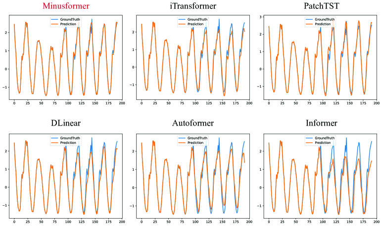
Figure 11: Prediction cases from the Traffic dataset under the input-96-predict-96 setting.

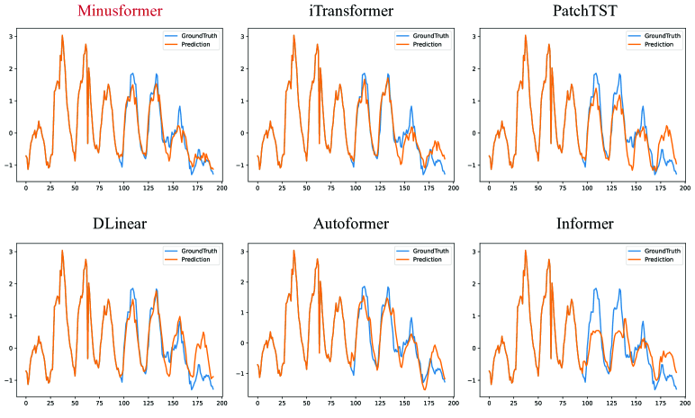
Figure 12: Prediction cases from the Electricity dataset under the input-96-predict-96 setting.

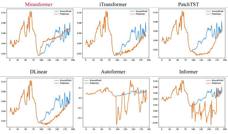
Figure 13: Prediction cases from the Weather dataset under the input-96-predict-96 setting.

Appendix G Full Univariate TS Forecasting Results

The full results for univariate TS forecasting are presented in Table 6. As other models, e.g., iTransformer (Liu et al., 2023), PatchTST (Nie et al., 2022) and Crossformer (Zhang & Yan, 2022) do not offer performance information for all prediction lengths, we compare our method with those that provide comprehensive performance analysis, including Periodformer (Liang et al., 2023), FEDformer (Zhou et al., 2022), Autoformer (Wu et al., 2021), Informer (Zhou et al., 2021), LogTrans (Li et al., 2019) and Reformer (Kitaev et al., 2020). Despite Periodformer being a model that determines optimal hyperparameters through search, the proposed method outperforms benchmark approaches by achieving the highest count of leading terms across various prediction lengths. This reaffirms the effectiveness of Minusformer.

Table 6: Univariate TS forecasting results on benchmark datasets.

Model		Minusformer-96		Periodformer-144♢		FEDformer-96		Autoformer-96		Informer-96		LogTrans-96		Reformer-96
	Length	MSE	MAE	MSE	MAE	MSE	MAE	MSE	MAE	MSE	MAE	MSE	MAE	MSE	MAE
ETTh1	96	0.055	0.177	0.068	0.203	0.079	0.215	0.071	0.206	0.193	0.377	0.283	0.468	0.532	0.569
	192	0.072	0.204	0.088	0.228	0.104	0.245	0.114	0.262	0.217	0.395	0.234	0.409	0.568	0.575
	336	0.08	0.219	0.105	0.256	0.119	0.270	0.107	0.258	0.202	0.381	0.386	0.546	0.635	0.589
	720	0.079	0.224	0.109	0.262	0.142	0.299	0.126	0.283	0.183	0.355	0.475	0.628	0.762	0.666
	Avg	0.072	0.206	0.093	0.237	0.111	0.257	0.105	0.252	0.199	0.377	0.345	0.513	0.624	0.600
ETTh2	96	0.129	0.275	0.125	0.272	0.128	0.271	0.153	0.306	0.213	0.373	0.217	0.379	1.411	0.838
	192	0.178	0.329	0.175	0.329	0.185	0.33	0.204	0.351	0.227	0.387	0.281	0.429	5.658	1.671
	336	0.211	0.365	0.219	0.372	0.231	0.378	0.246	0.389	0.242	0.401	0.293	0.437	4.777	1.582
	720	0.220	0.377	0.249	0.400	0.278	0.42	0.268	0.409	0.291	0.439	0.218	0.387	2.042	1.039
	Avg	0.185	0.337	0.192	0.343	0.206	0.350	0.218	0.364	0.243	0.400	0.252	0.408	3.472	1.283
ETTm1	96	0.029	0.126	0.033	0.139	0.033	0.140	0.056	0.183	0.109	0.277	0.049	0.171	0.296	0.355
	192	0.044	0.158	0.052	0.177	0.058	0.186	0.081	0.216	0.151	0.310	0.157	0.317	0.429	0.474
	336	0.057	0.185	0.070	0.267	0.084	0.231	0.076	0.218	0.427	0.591	0.289	0.459	0.585	0.583
	720	0.080	0.218	0.081	0.221	0.102	0.250	0.110	0.267	0.438	0.586	0.430	0.579	0.782	0.73
	Avg	0.052	0.172	0.059	0.201	0.069	0.202	0.081	0.221	0.281	0.441	0.231	0.382	0.523	0.536
ETTm2	96	0.064	0.180	0.060	0.182	0.063	0.189	0.065	0.189	0.08	0.217	0.075	0.208	0.077	0.214
	192	0.099	0.233	0.099	0.236	0.110	0.252	0.118	0.256	0.112	0.259	0.129	0.275	0.138	0.290
	336	0.129	0.273	0.129	0.275	0.147	0.301	0.154	0.305	0.166	0.314	0.154	0.302	0.160	0.313
	720	0.180	0.329	0.170	0.317	0.219	0.368	0.182	0.335	0.228	0.380	0.160	0.322	0.168	0.334
	Avg	0.118	0.254	0.115	0.253	0.135	0.278	0.130	0.271	0.147	0.293	0.130	0.277	0.136	0.288
Traffic	96	0.127	0.202	0.143	0.222	0.170	0.263	0.246	0.346	0.257	0.353	0.226	0.317	0.313	0.383
	192	0.135	0.211	0.146	0.227	0.173	0.265	0.266	0.37	0.299	0.376	0.314	0.408	0.386	0.453
	336	0.130	0.215	0.147	0.231	0.178	0.266	0.263	0.371	0.312	0.387	0.387	0.453	0.423	0.468
	720	0.135	0.218	0.164	0.252	0.187	0.286	0.269	0.372	0.366	0.436	0.437	0.491	0.378	0.433
	Avg	0.132	0.212	0.150	0.233	0.177	0.270	0.261	0.365	0.309	0.388	0.341	0.417	0.375	0.434
Electricity	96	0.249	0.358	0.236	0.349	0.262	0.378	0.341	0.438	0.258	0.367	0.288	0.393	0.275	0.379
	192	0.286	0.379	0.277	0.369	0.316	0.410	0.345	0.428	0.285	0.388	0.432	0.483	0.304	0.402
	336	0.337	0.413	0.324	0.400	0.361	0.445	0.406	0.470	0.336	0.423	0.430	0.483	0.37	0.448
	720	0.385	0.454	0.353	0.437	0.448	0.501	0.565	0.581	0.607	0.599	0.491	0.531	0.46	0.511
	Avg	0.314	0.401	0.298	0.389	0.347	0.434	0.414	0.479	0.372	0.444	0.410	0.473	0.352	0.435
Weather	96	0.0012	0.0263	0.0015	0.0300	0.0035	0.046	0.0110	0.081	0.004	0.044	0.0046	0.052	0.012	0.087
	192	0.0014	0.0283	0.0015	0.0307	0.0054	0.059	0.0075	0.067	0.002	0.040	0.006	0.060	0.0098	0.044
	336	0.0015	0.0294	0.0017	0.0313	0.008	0.072	0.0063	0.062	0.004	0.049	0.006	0.054	0.013	0.100
	720	0.002	0.0333	0.0020	0.0348	0.015	0.091	0.0085	0.070	0.003	0.042	0.007	0.059	0.011	0.083
	Avg	0.0015	0.0293	0.0017	0.0317	0.008	0.067	0.0083	0.0700	0.0033	0.0438	0.0059	0.0563	0.0115	0.0785
Exchange	96	0.096	0.226	0.092	0.226	0.131	0.284	0.241	0.387	1.327	0.944	0.237	0.377	0.298	0.444
	192	0.200	0.332	0.198	0.341	0.277	0.420	0.300	0.369	1.258	0.924	0.738	0.619	0.777	0.719
	336	0.400	0.473	0.370	0.471	0.426	0.511	0.509	0.524	2.179	1.296	2.018	1.0700	1.833	1.128
	720	1.020	0.779	0.753	0.696	1.162	0.832	1.260	0.867	1.28	0.953	2.405	1.175	1.203	0.956
	Avg	0.429	0.453	0.353	0.434	0.499	0.512	0.578	0.537	1.511	1.029	1.350	0.810	1.028	0.812
$1^{\text{st}}$ Count		24	27	14	12	0	1	0	0	0	0	2	0	0	0

• ${\diamondsuit}$ denotes the maximum search range of the input length.

References

- Anderson (1976) Anderson, O. D. Time-series. Journal of the Royal Statistical Society. Series D (The Statistician), 25(4):308–310, 1976. ISSN 00390526, 14679884.
- Castro-Neto et al. (2009) Castro-Neto, M., Jeong, Y.-S., Jeong, M.-K., and Han, L. D. Online-svr for short-term traffic flow prediction under typical and atypical traffic conditions. Expert Systems with Applications, 36(3):6164–6173, 2009.
- Cheng et al. (2015) Cheng, C., Sa-Ngasoongsong, A., Beyca, O., Le, T., Yang, H., Kong, Z., and Bukkapatnam, S. T. Time series forecasting for nonlinear and non-stationary processes: a review and comparative study. Iie Transactions, 47(10):1053–1071, 2015.
- Cleveland et al. (1990) Cleveland, R. B., Cleveland, W. S., McRae, J. E., and Terpenning, I. Stl: A seasonal-trend decomposition. J. Off. Stat, 6(1):3–73, 1990.
- Connor et al. (1994) Connor, J. T., Martin, R. D., and Atlas, L. E. Recurrent neural networks and robust time series prediction. IEEE Transactions on Neural Networks, 5(2):240–254, 1994.
- De Gooijer & Hyndman (2006) De Gooijer, J. G. and Hyndman, R. J. 25 years of time series forecasting. International journal of forecasting, 22(3):443–473, 2006.
- Gardner Jr (1985) Gardner Jr, E. S. Exponential smoothing: The state of the art. Journal of forecasting, 4(1):1–28, 1985.
- Hornik (1991) Hornik, K. Approximation capabilities of multilayer feedforward networks. Neural networks, 4(2):251–257, 1991.
- Hyndman & Athanasopoulos (2018) Hyndman, R. J. and Athanasopoulos, G. Forecasting: principles and practice. OTexts, 2018.
- Kingma & Ba (2015) Kingma, D. P. and Ba, J. Adam: A method for stochastic optimization. In International Conference on Learning Representations (ICLR), Santiago de Cuba, 2015.
- Kitaev et al. (2020) Kitaev, N., Kaiser, L., and Levskaya, A. Reformer: The efficient transformer. In 8th International Conference on Learning Representations (ICLR), Ababa, Ethiopia, 2020.
- Lai et al. (2018) Lai, G., Chang, W.-C., Yang, Y., and Liu, H. Modeling long- and short-term temporal patterns with deep neural networks. In The 41st international ACM SIGIR conference on research & development in information retrieval (SIGIR), pp. 95–104, Ann Arbor, MI, USA, 2018.
- LeCun et al. (1998) LeCun, Y., Bottou, L., Bengio, Y., and Haffner, P. Gradient-based learning applied to document recognition. Proceedings of the IEEE, 86(11):2278–2324, 1998.
- Li et al. (2023) Li, F., Feng, J., Yan, H., Jin, G., Yang, F., Sun, F., Jin, D., and Li, Y. Dynamic graph convolutional recurrent network for traffic prediction: Benchmark and solution. ACM Transactions on Knowledge Discovery from Data, 17(1):1–21, 2023.
- Li et al. (2010) Li, L., Prakash, B. A., and Faloutsos, C. Parsimonious linear fingerprinting for time series. Proceedings of the VLDB Endowment, 3(1-2):385–396, 2010.
- Li et al. (2019) Li, S., Jin, X., Xuan, Y., Zhou, X., Chen, W., Wang, Y.-X., and Yan, X. Enhancing the locality and breaking the memory bottleneck of transformer on time series forecasting. In Advances in 33rd Neural Information Processing Systems (NeurIPS), volume 32, pp. 5243–5253, Vancouver, Canada, 2019.
- Li et al. (2018) Li, Y., Yu, R., Shahabi, C., and Liu, Y. Diffusion convolutional recurrent neural network: Data-driven traffic forecasting. In International Conference on Learning Representations, 2018.
- Liang et al. (2023) Liang, D., Zhang, H., Yuan, D., Ma, X., Li, D., and Zhang, M. Does long-term series forecasting need complex attention and extra long inputs? arXiv preprint arXiv:2306.05035, 2023.
- Liaw et al. (2002) Liaw, A., Wiener, M., et al. Classification and regression by randomforest. R News, 2(3):18–22, 2002.
- Liu et al. (2022a) Liu, M., Zeng, A., Chen, M., Xu, Z., Lai, Q., Ma, L., and Xu, Q. Scinet: Time series modeling and forecasting with sample convolution and interaction. In Advances in Neural Information Processing Systems, pp. 5816–5828, 2022a.
- Liu et al. (2022b) Liu, Y., Wu, H., Wang, J., and Long, M. Non-stationary transformers: Exploring the stationarity in time series forecasting. Advances in Neural Information Processing Systems, 35:9881–9893, 2022b.
- Liu et al. (2023) Liu, Y., Hu, T., Zhang, H., Wu, H., Wang, S., Ma, L., and Long, M. itransformer: Inverted transformers are effective for time series forecasting. arXiv preprint arXiv:2310.06625, 2023.
- Nie et al. (2022) Nie, Y., Nguyen, N. H., Sinthong, P., and Kalagnanam, J. A time series is worth 64 words: Long-term forecasting with transformers. In The Eleventh International Conference on Learning Representations, 2022.
- Oreshkin et al. (2019) Oreshkin, B. N., Carpov, D., Chapados, N., and Bengio, Y. N-beats: Neural basis expansion analysis for interpretable time series forecasting. In International Conference on Learning Representations, 2019.
- Piccolo (1990) Piccolo, D. A distance measure for classifying arima models. Journal of time series analysis, 11(2):153–164, 1990.
- Salinas et al. (2020) Salinas, D., Flunkert, V., Gasthaus, J., and Januschowski, T. Deepar: Probabilistic forecasting with autoregressive recurrent networks. International Journal of Forecasting, 36(3):1181–1191, 2020.
- Shao et al. (2022) Shao, Z., Zhang, Z., Wang, F., Wei, W., and Xu, Y. Spatial-temporal identity: A simple yet effective baseline for multivariate time series forecasting. In Proceedings of the 31st ACM International Conference on Information & Knowledge Management, pp. 4454–4458, 2022.
- Taylor & Letham (2018) Taylor, S. J. and Letham, B. Forecasting at scale. The American Statistician, 72(1):37–45, 2018.
- Wu et al. (2021) Wu, H., Xu, J., Wang, J., and Long, M. Autoformer: Decomposition transformers with auto-correlation for long-term series forecasting. In Advances in Neural Information Processing Systems (NeurIPS), volume 34, pp. 22419–22430, Virtual Conference, 2021.
- Wu et al. (2022a) Wu, H., Hu, T., Liu, Y., Zhou, H., Wang, J., and Long, M. Timesnet: Temporal 2d-variation modeling for general time series analysis. In The Eleventh International Conference on Learning Representations, 2022a.
- Wu et al. (2022b) Wu, H., Wu, J., Xu, J., Wang, J., and Long, M. Flowformer: Linearizing transformers with conservation flows. In International Conference on Machine Learning, 2022b.
- Wu et al. (2019) Wu, Z., Pan, S., Long, G., Jiang, J., and Zhang, C. Graph wavenet for deep spatial-temporal graph modeling. In Proceedings of the Twenty-Eighth International Joint Conference on Artificial Intelligence. International Joint Conferences on Artificial Intelligence Organization, 2019.
- Yao et al. (2021) Yao, Y., Gu, B., Su, Z., and Guizani, M. Mvstgn: A multi-view spatial-temporal graph network for cellular traffic prediction. IEEE Transactions on Mobile Computing, 2021.
- Zeng et al. (2023) Zeng, A., Chen, M., Zhang, L., and Xu, Q. Are transformers effective for time series forecasting? In Proceedings of the AAAI conference on artificial intelligence, volume 37, pp. 11121–11128, 2023.
- Zhang & Yan (2022) Zhang, Y. and Yan, J. Crossformer: Transformer utilizing cross-dimension dependency for multivariate time series forecasting. In The Eleventh International Conference on Learning Representations, 2022.
- Zhou et al. (2021) Zhou, H., Zhang, S., Peng, J., Zhang, S., Li, J., Xiong, H., and Zhang, W. Informer: Beyond efficient transformer for long sequence time-series forecasting. In Proceedings of the 35th AAAI Conference on Artificial Intelligence (AAAI), volume 35, pp. 11106–11115, Virtual Conference, 2021.
- Zhou et al. (2022) Zhou, T., Ma, Z., Wen, Q., Wang, X., Sun, L., and Jin, R. FEDformer: Frequency enhanced decomposed transformer for long-term series forecasting. In Proceedings of the 39th International Conference on Machine Learning (ICML), volume 162, pp. 27268–27286, Baltimore, Maryland, 2022.