Role of Momentum in Smoothing Objective Function
in Implicit Graduated Optimization

Abstract

While stochastic gradient descent (SGD) with momentum has fast convergence and excellent generalizability, a theoretical explanation for this is lacking. In this paper, we show that SGD with momentum smooths the objective function, the degree of which is determined by the learning rate, the batch size, the momentum factor, the variance of the stochastic gradient, and the upper bound of the gradient norm. This theoretical finding reveals why momentum improves generalizability and provides new insights into the role of the hyperparameters, including momentum factor. We also present an implicit graduated optimization algorithm that exploits the smoothing properties of SGD with momentum and provide experimental results supporting our assertion that SGD with momentum smooths the objective function.

1 Introduction

1.1 Background

First-order optimizers that use mini-batch stochastic gradients, such as stochastic gradient descent (SGD) [50], SGD with momentum [48, 46], and adaptive methods [12, 31], are the most commonly used methods for solving empirical risk minimization problems that appear in machine learning. These methods have been well studied for their convergence [3, 4, 7, 13, 25, 40, 54, 63, 65, 67] and stability [19, 22, 38, 45], and it has been shown that tuning the hyperparameters such as the learning rate, batch size, and momentum factor is essential for successful training. This paper focuses on the SGD with momentum method and provides new insights into its convergence and stability and the role of the momentum factor.

For nonconvex objective functions, including deep neural networks (DNNs), SGD with momentum experimentally converges faster than SGD without momentum (simply ”SGD” hereafter) and has better generalizability, but theoretical explanations for these characteristics have not yet been provided. Although convergence analyses of SGD with momentum for nonconvex functions have been provided [16, 39, 11], none of them explain why convergence is faster than with SGD. The generalizability of SGD with momentum has been well studied, and various experimental findings have been reported. While it has been suggested that momentum plays a role in reducing stochastic noise [11, 8], stochastic noise has been shown to increase generalizability [37, 59, 18], and it has been claimed that stochastic noise can help an algorithm escape from local solutions with poor generalizability [15, 28, 10, 20, 32]. Furthermore, many studies [56, 27, 34] have shown that the gap in convergence speed and generalizability between SGD and SGD with momentum is more pronounced for large batches. There is an inconsistency in that adding momentum should reduce stochastic noise, but because momentum has excellent generalizability, it should have sufficiently large noise, and this contradiction makes it difficult to understand the effect of momentum in DNNs.

Figure 1: Conceptual diagram of new $\sigma$-nice function and its smoothed versions (see notation in Table 1).

The simplest method for adding a momentum term to SGD is the stochastic heavy ball (SHB) method (Algorithm 1) [48]. Although it has been widely used in experiments, it is lacking in theoretical analysis. In contrast, the normalized-SHB (NSHB) method (Algorithm 2 with $\nu=1$) [17] has been well analyzed theoretically for convergence and stability but has rarely been used in experiments. Note that the algorithm referred to as “SGD with momentum (SGDM)” in many previous studies is actually NSHB, while that provided by PyTorch [47] is SHB. Many variants of the momentum method have been proposed, including Nesterov’s accelerated gradient method [58], synthesized Nesterov variants [36], Triple Momentum [55], Robust Momentum [9], PID control-based methods [1], accelerated SGD [30], and quasi-hyperbolic momentum (QHM, Algorithm 2) [42]. This paper focuses on SHB and QHM, which covers many momentum methods, especially NSHB, but does not cover SHB.

Graduated optimization and new $\sigma$-nice function. Graduated optimization [2, 51, 61] is a global optimization approach in which multiple objective functions smoothed with progressively smaller noise are optimized sequentially, starting with the smoothest function. The objective is to search for a global optimal solution while avoiding a local optimal solution of the original objective function. Hazan et al. defined and provided an analysis of $\sigma$-nice functions, a special family of nonconvex functions that satisfy certain conditions that guarantee convergence to a global optimal solution [21]. Sato and Iiduka proposed the new $\sigma$-nice function, which is an extension of the $\sigma$-nice function, and showed that SGD has the effect of smoothing the objective function, the degree of which is determined by the learning rate, batch size, and variance of the stochastic gradient [53]. Furthermore, they proposed an implicit graduated optimization algorithm using SGD with a decaying learning rate or increasing batch size and showed that this algorithm can reach a global optimal solution in $\mathcal{O}\left(1/\epsilon^{\frac{1}{p}}\right)(p\in(0,1])$ iterations for the new $\sigma$-nice function.

1.2 Motivation

Sato and Iiduka provided new insights into the role of the learning rate and batch size through analysis of implicit graduated optimization for the new $\sigma$-nice function [53]. We first extend the implicit graduated optimization approach to momentum to see if there is a smoothing effect on SHB and QHM and discuss which parameters determine the degree of smoothing. Through this analysis, we aim to gain a theoretical understanding of the role of momentum, batch size, and learning rate in DNNs and clarify why and when momentum is effective. Finally, we construct an implicit graduated optimization algorithm using the smoothing properties of SHB and QHM to achieve global optimization of DNNs.

Table 1: Notation

Notation	Description
$\mathbb{N}$	The set of all nonnegative integers
$[N]$	$[N]:=\{1,2,\ldots,N\}$ ($N\in\mathbb{N}\backslash\{0\}$)
$\mathbb{R}^{d}$	A $d$-dimensional Euclidean space with inner product $\langle\cdot,\cdot\rangle$, which induces the norm $\|\cdot\|$
$\mathbb{E}_{\xi}[X]$	The expectation with respect to $\xi$ of a random variable $X$
$\mathcal{S}_{t}$	Mini-batch of $b$ samples $\bm{z}_{i}$ at time $t$
$N(\bm{x}^{\star};\epsilon)$	$\epsilon$-neighborhood of a vector $\bm{x}^{\star}$, i.e., $N(\bm{x}^{\star};\epsilon):=\left\{\bm{x}\in\mathbb{R}^{d}\colon\|\bm{x}-\bm{x}^{\star}\|<\epsilon\right\}$
$B(\bm{x}^{\star};r)$	The Euclidian closed ball of radius $r$ centered at $\bm{x}^{\star}$, i.e., $B(\bm{x}^{\star};r):=\left\{\bm{x}\in\mathbb{R}^{d}\colon\|\bm{x}-\bm{x}^{\star}\|\leq r\right\}$
$\bm{u}\sim B(\bm{x}^{\star};r)$	A random variable distributed uniformly over $B(\bm{x}^{\star};r)$
$f_{i}(\bm{x})$	A loss function for $\bm{x}\in\mathbb{R}^{d}$ and sample $\bm{z}_{i}\ (i\in[n])$
$f(\bm{x})$	The total loss function for $\bm{x}\in\mathbb{R}^{d}$, i.e., $f(\bm{x}):=\frac{1}{n}\sum_{i\in[n]}f_{i}(\bm{x})$
$\xi$	A random variable supported on $\Xi$ that does not depend on $\bm{x}\in\mathbb{R}^{d}$
$\bm{\xi}_{t}$	$\xi_{0},\xi_{1},\ldots$ are independent samples and $\xi_{t}$ is independent of $(\bm{x}_{k})_{k=0}^{t}\subset\mathbb{R}^{d}$
$\xi_{t,i}$	A random variable generated from the $i$-th sampling at time $t$
$\mathsf{G}_{\bm{\xi}_{t}}(\bm{x})$	The stochastic gradient of $f(\cdot)$ at $\bm{x}\in\mathbb{R}^{d}$
$\nabla f_{\mathcal{S}_{t}}(\bm{x}_{t})$	The mini-batch stochastic gradient of $f(\bm{x}_{t})$ for $\mathcal{S}_{t}$, i.e., $\nabla f_{\mathcal{S}_{t}}(\bm{x}_{t}):=b^{-1}\sum_{i\in[b]}\mathsf{G}_{\xi_{t,i}}(\bm{x}_{t})$
$M$	The number of smoothed functions, i.e., $M\in\mathbb{N}$
$m$	Counts from the smoothest function, i.e., $m\in[M]$
$\delta$	The degree of smoothing of the smoothed function, i.e., $\delta\in\mathbb{R}$
$\delta_{m}$	The degree of smoothing of the $m$-th smoothed function, i.e., $\delta_{m}\in\mathbb{R}$
$\hat{f}_{\delta}$	The function obtained by smoothing $f$ with a noise level $\delta$
$\hat{f}_{\delta_{m}}$	The $m$-th smoothed function obtained by smoothing $f$ with a noise level $\delta_{m}$
$\bm{x}_{m+1}$	$\bm{x}_{m+1}$ is defined by $\hat{f}_{\delta_{m}}(\bm{x}_{m+1})\leq\hat{f}_{\delta_{m}}(\hat{\bm{x}}_{t})$, where $(\hat{\bm{x}}_{t})_{t=1}^{T_{F}+1}$ is generated by $\text{GD}(T_{F},\bm{x}_{m},\hat{f}_{\delta_{m}},\eta_{m})$

1.3 Contributions

Estimation of critical batch size and variance of stochastic gradient. We show the existence of a critical batch size in the training of a DNN with SGD and SGD with momentum and provide a formula for estimating the size. We also estimate the variance of the stochastic gradient for an optimizer from the experimentally estimated critical batch size and show that SGD with momentum, especially SHB, has a smaller variance than SGD. This is the first paper to provide a formula for estimating the critical batch size for SGD and SGD with momentum, and, to the best of our knowledge, the first attempt to estimate the variance of stochastic gradients.

SGD with momentum’s smoothing property. We show that SGD with momentum also has a smoothing effect on the objective function, the degree of which is determined by the momentum factor, the variance of the stochastic gradient, and the upper bound of the gradient norm, in addition to the learning rate and batch size. We also show that a large learning rate and/or small batch size, and/or a large momentum factor, smooths the function even more (see Figure 1). Although their results were derived from a different perspective, Smith et al. obtained similar results [57]. Furthermore, the results of several experimental studies suggest that these hyperparameters are interrelated [30, 35, 34, 14]. Our results provide theoretical support for these and new insights into the role of hyperparameters in DNN training.

Why and when momentum improves generalizability. Smoothing of the objective function with sufficiently large noise avoids sharp local optimal solutions and leads to a flat local optimal solution [53]. Thus, we suggest that the generalizability of SGD with momentum is superior to that of SGD because SGD with momentum almost always has a greater degree of smoothing than SGD (see Figure 3). We show that the degree of smoothing in SGD with momentum does not decrease much with increasing batch size, in contrast to SGD. Therefore, the reason SGD with momentum has high generalization performance even with large batch sizes is that the degree of smoothing is sufficiently large even with large batch sizes. Experiments have shown that the generalization performance of SGD with momentum does not worsen much even when the batch size is large [34, 56, 27], in contrast to that of SGD, and our results provide theoretical support for this finding.

Implicit graduated optimization with momentum. We present a new implicit graduated optimization algorithm that exploits the smoothing effect of SGD with momentum and show that our algorithm for the $L_{f}$-Lipschitz new $\sigma$-nice function converges to an $\epsilon$-neighborhood of the global optimal solution in $\mathcal{O}\left(1/\epsilon^{\frac{1}{p}}\right)\ (p\in(0,1])$. In Section 4.3, we show experimentally that our algorithm is superior to SGD with momentum with constant parameters on image classification tasks.

2 Preliminaries

2.1 Assumptions

The notations used in this paper are summarized in Table 1. We make the following assumptions:

Assumption 2.1.

(A1) $f_{i}\colon\mathbb{R}^{d}\to\mathbb{R}\ (i\in[n])$ is continuously differentiable.

(A2) $(\bm{x}_{t})_{t\in\mathbb{N}}\subset\mathbb{R}^{d}$ is a sequence generated by an optimizer.

(i) For each iteration $t$,  $\mathbb{E}_{\bm{\xi}_{t}}\left[\mathsf{G}_{\bm{\xi}_{t}}(\bm{x}_{t})\right]=\nabla f(\bm{x}_{t}).$

(ii) There exists a nonnegative constant $C_{\text{\rm{opt}}}^{2}$ for an optimizer such that $\mathbb{E}_{\bm{\xi}_{t}}\left[\|\mathsf{G}_{\xi_{t}}(\bm{x}_{t})-\nabla f(\bm{x}_{t})\|^{2}\right]\leq C_{\text{\rm{opt}}}^{2}$.

(A3) For each iteration $t$, the optimizer samples a mini-batch $\mathcal{S}_{t}\subset\mathcal{S}$ and estimates the full gradient $\nabla f$ as $\nabla f_{\mathcal{S}_{t}}(\bm{x}_{t}):=\frac{1}{b}\sum_{i\in[b]}\mathsf{G}_{\xi_{t,i}}(\bm{x}_{t})=\frac{1}{b}\sum_{\{i\colon\bm{z}_{i}\in\mathcal{S}_{t}\}}\nabla f_{i}(\bm{x}_{t})$.

(A4) There exists a positive constant $K_{\text{\rm{opt}}}$ for an optimizer, for all $t\in\mathbb{N}$, $\mathbb{E}\left[\|\nabla f(\bm{x}_{t})\|^{2}\right]\leq K_{\text{\rm{opt}}}^{2}$, where $\mathbb{E}\left[\cdot\right]$ stands for the total expectation.

The variance of the stochastic gradient and the upper bound of the gradient are often assumed to be constant for any optimizer, but we define it for each optimizer.

2.2 Algorithms

We consider two algorithms that are a type of SGD with momentum.

Algorithm 1 Stochastic Heavy Ball (SHB)

0:  $\bm{x}_{0},\eta>0,\beta\in[0,1),\bm{m}_{-1}:=\bm{0}$

  for $t=0$ to $T-1$ do

     $\bm{m}_{t}:=\nabla f_{\mathcal{S}_{t}}(\bm{x}_{t})+\beta\bm{m}_{t-1}$

     $\bm{x}_{t+1}:=\bm{x}_{t}-\eta\bm{m}_{t}$

  end for

  return  $\bm{x}_{T}$

Algorithm 2 Quasi-Hyperbolic Momentum (QHM)

0:  $\bm{x}_{0},\eta>0,\beta\in[0,1),\nu\in[0,1],\bm{d}_{-1}:=\bm{0}$

  for $t=0$ to $T-1$ do

     $\bm{d}_{t}:=(1-\nu\beta)\nabla f_{\mathcal{S}_{t}}(\bm{x}_{t})+\nu\beta\bm{d}_{t-1}$

     $\bm{x}_{t+1}:=\bm{x}_{t}-\eta\bm{d}_{t}$

  end for

  return  $\bm{x}_{T}$

In accordance with Gitman et al.[16], we refer to Algorithm 1 as the stochastic heavy ball method. In Algorithm 2, $\nu$ is the coefficient balancing SGD ($\nu=0$) with NSHB ($\nu=1$).

3 Theoretical Analysis of SHB and QHM

We use convergence analysis of SHB and QHM in order to clarify the relationship between batch size and the number of steps required for training. We then provide an equation for estimating the critical batch size and the variance of the stochastic gradient for an optimizer. To analyze SHB and QHM, we further assume that,

Assumption 3.1.

(S1) For all $\bm{x}\in\mathbb{R}^{d}$, there exists a positive constant $D(\bm{x})$ such that

$$\|\bm{x}_{t}-\bm{x}\|\leq D(\bm{x}).$$

Assumption (S1) has been used to provide upper bounds on the performance measures when analyzing both convex and nonconvex optimization of DNNs [31, 49, 66].

3.1 Convergence analysis of SHB and QHM

We first present convergence analysis of Algorithm 1 (The proof of Theorem 3.1 is in Appendix A.3).

Theorem 3.1.

Suppose that Assumptions (A1)$-$(A4) and (S1) hold and consider the sequence $(\bm{x}_{t})_{t\in\mathbb{N}}$ generated by SHB. Then, for all $\bm{x}\in\mathbb{R}^{d}$ and all $T\geq 1$, the following holds:

$$\frac{1}{T}\sum_{t=0}^{T-1}\mathbb{E}\left[\langle\bm{x}_{t}-\bm{x},\nabla f(\bm{x}_{t})\rangle\right]$$

$$\quad\leq\frac{\|\bm{x}_{0}-\bm{x}\|^{2}}{2\eta T}+\frac{\beta D(\bm{x})}{1-\beta}\sqrt{\frac{C_{\text{\rm{SHB}}}^{2}}{b}+K_{\text{\rm{SHB}}}^{2}}$$

$$\quad\quad+\frac{\eta\left(\beta^{2}-\beta+1\right)}{2\beta(1-\beta)^{2}}\left(\frac{C_{\text{\rm{SHB}}}^{2}}{b}+K_{\text{\rm{SHB}}}^{2}\right).$$

We next present convergence analysis of Algorithm 2 (The proof of Theorem 3.2 is in Appendix A.5).

Theorem 3.2.

Suppose that Assumptions (A1)$-$(A4) and (S1) hold and consider the sequence $(\bm{x}_{t})_{t\in\mathbb{N}}$ generated by QHM. Then, for all $\bm{x}\in\mathbb{R}^{d}$ and all $T\geq 1$, the following holds:

$$\frac{1}{T}\sum_{t=0}^{T-1}\mathbb{E}\left[\langle\bm{x}_{t}-\bm{x},\nabla f(\bm{x}_{t})\rangle\right]$$

$$\quad\leq\frac{\|\bm{x}_{0}-\bm{x}\|^{2}}{2\eta(1-\nu\beta)T}+\frac{\nu\beta D(\bm{x})}{1-\nu\beta}\sqrt{\frac{C_{\text{\rm{QHM}}}^{2}}{b}+K_{\text{\rm{QHM}}}^{2}}$$

$$\quad\quad+\frac{\eta}{2(1-\nu\beta)}\left(\frac{C_{\text{\rm{QHM}}}^{2}}{b}+K_{\text{\rm{QHM}}}^{2}\right).$$

Convergence analysis for NSHB is performed using Theorem 3.2 with $\nu=1$.

3.2 Estimation of critical batch size

Previous studies [56, 43, 44] have shown experimentally that the number of steps $T$ required to train a DNN is halved when batch size $b$ is doubled, but this phenomenon is not observed beyond a critical batch size. Therefore, the critical batch size is the batch size that minimizes the computational complexity for training. Zhang et al. suggested that the critical batch size depends on the optimizer [64], and Iiduka and Sato theoretically proved its existence and provided a formula for estimating its lower bound from the hyperparameters [26, 52].

From Theorems A.1, 3.1, and 3.2, we can derive the following proposition, which gives a lower bound on the critical batch size $b_{\text{\rm}{opt}}^{\star}$. For a proof of Proposition 3.1 and a more detailed discussion of its derivation, see Appendix B.

Proposition 3.1.

Suppose that Assumptions (A1)$-$(A4) and (S1) hold and consider SGD, SHB, and QHM. Then, the following hold:

$$b_{\text{\rm{SGD}}}^{\star}>\frac{\eta C_{\text{\rm{SGD}}}^{2}}{\epsilon^{2}},$$

$$b_{\text{\rm{SHB}}}^{\star}>\frac{\eta(\beta^{2}-\beta+1)C_{\text{\rm{SHB}}}^{2}}{\beta(1-\beta)^{2}\epsilon^{2}},$$

$$b_{\text{\rm{QHM}}}^{\star}>\frac{\eta C_{\text{\rm{QHM}}}^{2}}{(1-\nu\beta)\epsilon^{2}}.$$

Proposition 3.1 provides a formula for estimating a lower bound for the critical batch size, but in practice it is impossible to estimate the critical batch size completely in advance because it involves an unknown, $C_{\text{\rm{opt}}}^{2}$. However, this is a very important proposition because it connects theory and experiment, and we can use it to back-calculate the variance of the stochastic gradient $C_{\text{\rm{opt}}}^{2}$ (see Section 3.3).

3.3 Numerical results

We experimentally demonstrated the existence of a critical batch size. For different batch sizes, we measured the number of steps required for the gradient norm of the past $t$ steps at time $t$ to average less than $0.5$ in training ResNet18 [23] on the CIFAR100 dataset [33]. See Appendix B.4 for more details on the experiments discussed in this section and similar results on WideResNet-28-10 [62].

Learning rate $\eta$ of $0.1$ was used for all optimizers, with a momentum factor $\beta$ of $0.9$ for SHB and NSHB. Figure 2 plots stochastic first-order oracle (SFO) complexity $Tb$ versus $b$. The estimated critical batch sizes for SGD, SHB, and NSHB were $2^{9}$, $2^{10}$, and $2^{9}$, respectively.

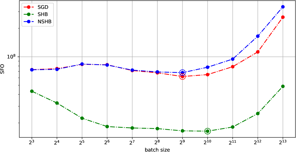
Figure 2: SFO complexities for SGD, SHB, and NSHB needed to train ResNet18 on CIFAR100 dataset versus batch size. The double circle symbols denote the critical batch sizes that minimize SFO complexity.

From Proposition 3.1 and these experimental results, we can estimate an upper bound on the variance of the stochastic gradient. For example, the variance of the stochastic gradient of SGD for training ResNet18 on the CIFAR100 dataset can be obtained as

$$C_{\text{\rm{SGD}}}^{2}<\frac{b_{\text{SGD}}^{\star}\epsilon^{2}}{\eta}=\frac{2^{9}\cdot(0.5)^{2}}{0.1}=1280.$$

Similar calculations for SHB and NSHB lead to $C_{\text{\rm{SHB}}}^{2}<25.3$ and $C_{\text{\rm{NSHB}}}^{2}<128$ (see Appendix B.5). Thus, adding a momentum term reduces the variance of the stochastic gradient, and the effect is seen especially in SHB. We also experimentally observed an upper bound on the gradient norm (see Assumption (A4)) for training ResNet18 on the CIFAR100 dataset: $K_{\text{\rm{SGD}}}=4.528$, $K_{\text{\rm{SHB}}}=1.77$, and $K_{\text{\rm{NSHB}}}=4.5$ (see Appendix B.5). These values are used in our discussion of the smoothing property of SGD with momentum in Section 4.1.

4 Graduated Optimization with Momentum

Sato and Iiduka showed that SGD with a mini-batch stochastic gradient has the effect of smoothing the function, and the degree of smoothing is determined by $\frac{\eta C}{\sqrt{b}}$, where $\eta$ is the learning rate and $b$ is the batch size [53]. In this section, we show that SHB (Algorithm 1) and QHM (Algorithm 2), which are SGD with momentum, also have the effect of smoothing the function and discuss the parameters that determine the degree of smoothing. Finally, this property is used to construct an implicit graduated optimization algorithm.

In general, smoothing of a function is achieved by convolving the function with a random variable that follows a normal or uniform distribution:

Definition 4.1 (Smoothed function).

Given an $L_{f}$-Lipschitz function $f$, define $\hat{f}_{\delta}$ to be the function obtained by smoothing $f$ as

$$\hat{f}_{\delta}(\bm{x}):=\mathbb{E}_{\bm{u}\sim B(\bm{0};1)}\left[f(\bm{x}-\delta\bm{u})\right],$$

where $\delta\in\mathbb{R}$ represents the degree of smoothing and $\bm{u}$ is a random variable distributed uniformly over $B(\bm{0};1)$. Also,

$$\bm{x}^{\star}:=\underset{\bm{x}\in\mathbb{R}^{d}}{\operatorname{argmin}}f(\bm{x})\text{\ \ and \ }\bm{x}_{\delta}^{\star}:=\underset{\bm{x}\in\mathbb{R}^{d}}{\operatorname{argmin}}\hat{f}_{\delta}(\bm{x}).$$

We focus on the new $\sigma$-nice function:

Definition 4.2 (new $\sigma$-nice function).

A function $f\colon\mathbb{R}^{d}\to\mathbb{R}$ is said to be “new $\sigma$-nice” if the following two conditions hold:

(i) For all $\delta_{m}\in\mathbb{R}\ (m\in[M])$, and all $\bm{x}_{\delta_{m}}^{\star}$,

$$\left\|\bm{x}_{\delta_{m}}^{\star}-\bm{x}_{\delta_{m+1}}^{\star}\right\|\leq|\delta_{m}|-|\delta_{m+1}|,$$

where $|\delta_{m+1}|:=\gamma_{m}|\delta_{m}|\ \left(\gamma_{m}\in\left(\frac{1}{d_{m+1}},1\right),d_{m}>1\right)$.

(ii) For all $\delta_{m}\in\mathbb{R}\ (m\in[M])$, the function $\hat{f}_{\delta_{m}}(\bm{x})$ is $\sigma$-strongly convex on $N(\bm{x}^{\star};d_{m}\delta_{m})$.

To analyze the new $\sigma$-nice function, we make two additional assumptions.

Assumption 4.1.

(C1) $f\colon\mathbb{R}^{d}\to\mathbb{R}$ is $L_{g}$-smooth, i.e.,

$$\forall\bm{x},\bm{y}\in\mathbb{R}^{d}:\|\nabla f(\bm{x})-\nabla f(\bm{y})\|\leq L_{g}\|\bm{x}-\bm{y}\|.$$

(C2) $f\colon\mathbb{R}^{d}\to\mathbb{R}$ is an $L_{f}$-Lipschitz function, i.e.,

$$\forall\bm{x},\bm{y}\in\mathbb{R}^{d}:\left|f(\bm{x})-f(\bm{y})\right|\leq L_{f}\|\bm{x}-\bm{y}\|.$$

4.1 SGD with momentum smoothing

At time $t$, let $\bm{\omega}_{t}^{\text{\rm{SHB}}}$ be the difference between the search direction of the gradient descent and the search direction of SHB, and let $\bm{\omega}_{t}^{\text{\rm{QHM}}}$ be the difference between the search direction of the gradient descent and the search direction of QHM, i.e.,

$$\bm{\omega}_{t}^{\text{\rm{SHB}}}:=\bm{m}_{t}-\nabla f(\bm{x}_{t})\text{\ \ and \ }\bm{\omega}_{t}^{\text{\rm{QHM}}}:=\bm{d}_{t}-\nabla f(\bm{x}_{t}).$$

Then, the following proposition holds:

Proposition 4.1.

Suppose that Assumptions (A2)(ii), (A3), and (A4) hold, then, for all $t\in\mathbb{N}$,

$$\mathbb{E}\left[\left\|\bm{\omega}_{t}^{\text{\rm{SHB}}}\right\|\right]\leq\sqrt{\left(1+\hat{\beta}\right)\frac{C_{\text{\rm{SHB}}}^{2}}{b}+\hat{\beta}K_{\text{\rm{SHB}}}^{2}},$$

$$\mathbb{E}\left[\left\|\bm{\omega}_{t}^{\text{\rm{QHM}}}\right\|\right]\leq\sqrt{\left(1+4\nu^{2}\beta^{2}\right)\frac{C_{\text{\rm{QHM}}}^{2}}{b}+4\nu^{2}\beta^{2}K_{\text{\rm{QHM}}}^{2}},$$

where $\hat{\beta}:=\frac{\beta(\beta^{2}-\beta+1)}{(1-\beta)^{2}}$.

Hence, $\bm{\omega}_{t}^{\text{\rm{SHB}}}$ and $\bm{\omega}_{t}^{\text{\rm{QHM}}}$ can be expressed as

$$\bm{\omega}_{t}^{\text{\rm{SHB}}}=\sqrt{\left(1+\hat{\beta}\right)\frac{C_{\text{\rm{SHB}}}^{2}}{b}+\hat{\beta}K_{\text{\rm{SHB}}}^{2}}\bm{u}_{t}=:\psi^{\text{SHB}}\bm{u}_{t},$$

$$\bm{\omega}_{t}^{\text{\rm{QHM}}}=\sqrt{\left(1+4\nu^{2}\beta^{2}\right)\frac{C_{\text{\rm{QHM}}}^{2}}{b}+4\nu^{2}\beta^{2}K_{\text{\rm{QHM}}}^{2}}\bm{u}_{t},$$

where $\bm{u}_{t}\sim B(\bm{0};1)$. In addition, let $\bm{y}_{t}$ be the parameter updated by the gradient descent and $\bm{x}_{t+1}$ be the parameter updated by SHB at time $t$; i.e.,

$$\bm{y}_{t} :=\bm{x}_{t}-\eta\nabla f(\bm{x}_{t}),$$

$$\bm{x}_{t+1} :=\bm{x}_{t}-\eta\bm{m}_{t}$$

$$=\bm{x}_{t}-\eta(\nabla f(\bm{x}_{t})+\bm{\omega}_{t}^{\text{\rm{SHB}}}).$$

Then, according to Definition 4.1, we have

$$\mathbb{E}_{\bm{\omega}_{t}^{\text{\rm{SHB}}}}\left[\bm{y}_{t+1}\right] =\bm{y}_{t}-\eta\nabla\mathbb{E}_{\bm{\omega}_{t}^{\text{\rm{SHB}}}}\left[f\left(\bm{y}_{t}-\eta\bm{\omega_{t}^{\text{SHB}}}\right)\right]$$ (1)

$$=\bm{y}_{t}-\eta\nabla\mathbb{E}_{\bm{u}_{t}\sim B(\bm{0};1)}\left[f(\bm{y}_{t}-\psi^{\text{SHB}}\bm{u}_{t})\right]$$

$$=\bm{y}_{t}-\eta\nabla\hat{f}_{\eta\psi^{\text{SHB}}}(\bm{y}_{t}).$$

(The derivation of equation (1) is presented in Appendix C.2.) This shows that the function $\mathbb{E}_{\bm{\omega}_{t}^{\text{\rm{SHB}}}}\left[f\left(\bm{y}_{t}-\eta\bm{\omega_{t}^{\text{SHB}}}\right)\right]$ is a smoothed version of $f$ with noise level $\eta\psi^{\text{SHB}}$. Furthermore, optimizing function $f$ with SHB is approximately equivalent to optimizing function $\hat{f}_{\eta\psi^{\text{SHB}}}$ with the gradient descent. Therefore, we can say that the degree of smoothing due to stochastic noise in SHB is determined by $\delta^{\text{SHB}}=\eta\psi^{\text{SHB}}$, i.e., learning rate $\eta$, batch size $b$, momentum factor $\beta$, the variance of stochastic gradient $C_{\text{\rm{SHB}}}$, and the upper bound of full gradient $K_{\text{\rm{SHB}}}$ for SHB. The same argument holds for QHM. The degree of smoothing for each optimizer can be expressed as

$$\delta^{\text{\rm{SGD}}}=\eta\sqrt{\frac{C_{\text{\rm{SGD}}}^{2}}{b}},$$ (2)

$$\delta^{\text{\rm{SHB}}}=\eta\sqrt{\frac{C_{\text{\rm{SHB}}}^{2}}{b}+\frac{\beta(\beta^{2}-\beta+1)}{(1-\beta)^{2}}\left(\frac{C_{\text{\rm{SHB}}}^{2}}{b}+K_{\text{\rm{SHB}}}^{2}\right)},$$ (3)

$$\delta^{\text{\rm{QHM}}}=\eta\sqrt{\frac{C_{\text{\rm{QHM}}}^{2}}{b}+4\nu^{2}\beta^{2}\left(\frac{C_{\text{\rm{QHM}}}^{2}}{b}+K_{\text{\rm{QHM}}}^{2}\right)},$$ (4)

and if $\nu=1$ in $\delta^{\text{\rm{QHM}}}$, we obtain $\delta^{\text{\rm{NSHB}}}$. Using the value of the variance of the stochastic gradient and the upper bound of the gradient norm obtained in Section 3.3, we can obtain the degree of smoothing for each batch size. Figure 3 plots the degree of smoothing when $\eta=0.1$ and $\beta=0.9$ versus batch size, and Figure 1 shows the relationships among the degree of smoothing, the learning rate, the batch size, and the momentum factor.

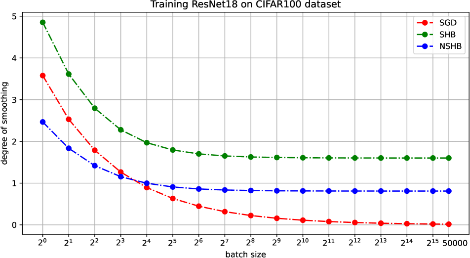
Figure 3: Degree of smoothing $\delta^{\text{\rm{SGD}}}$, $\delta^{\text{\rm{SHB}}}$, and $\delta^{\text{\rm{NSHB}}}$ when $\eta=0.1$ and $\beta=0.9$ for SGD, SHB, and NSHB versus batch size in training ResNet18 on CIFAR100 dataset. See Appendix C.3 for details on calculating the degree of smoothing and a logarithmic graph version.

The finding that the objective function is smoothed to some degree simply by using SGD with momentum is sufficient to address the following outstanding issues:

Why and when momentum improves generalizability. Sato and Iiduka showed that when the degree of smoothing is sufficiently large, the objective function can be smoothed significantly, and generalizability is improved because local optimal solutions can be avoided [53]. Figure 3 shows that the degree of smoothing in SGD with momentum is almost always greater than in SGD. Therefore, we conclude that SGD with momentum improves generalizability due to a greater degree of smoothing, even at the same learning rate and batch size as SGD. In addition to the momentum factor, Equations (3) and (4) show that hyperparameters such as the learning rate and batch size also contribute to smoothing (see Figure 1). Therefore, the learning rate, the batch size, and the momentum factor are interrelated, and they should be selected such that the degree of smoothing is appropriate. This finding is helpful in selecting appropriate hyperparameters. For example, if a large learning rate is used, a small momentum should obviously be used. Leclerc and Madry observed this phenomenon experimentally [35, Figure 4].

Why momentum has sufficient generalizability even with large batch sizes. Keskar et al. showed in their experiments that using SGD with large batch sizes leads to sharp local optimal solutions and worse generalization performance [29]. Using Equation (2), Sato and Iiduka demonstrated that large batch sizes tend to lead to sharp local optimal solutions due to insufficient smoothing of the objective function, whereas small batch sizes lead to high generalizability since they avoid sharp local solutions and reach flat optimal solutions due to large smoothing of the objective function. Figure 3 shows that the degree of smoothing in SHB and NSHB does not decrease with increasing batch size. Thus, in contrast to SGD, SGD with momentum attains sufficient smoothing even for large batch sizes so that generalizability does not worsen as the batch size increases.

Decaying learning rate and momentum factor in SGD with momentum is implicit graduated optimization. In contrast to SGD, for SHB and NSHB, Equations (3) and (4) suggest that using a decaying learning rate and/or decaying momentum factor is implicit graduated optimization. Note that increasing the batch size does not contribute to decreasing the degree of smoothing due to terms that are independent of batch size in both equations. Thus, a decrease in the learning rate and momentum lead to avoidance of sharp local optimal solutions, low loss function values, and high generalizability. There have been many attempts to reduce the learning rate [41, 24, 60, 6] or momentum factor [5], and its superiority has been shown experimentally, but there has been no theoretical explanation for them. Our discussion provides theoretical support for these.

4.2 Implicit graduated optimization with momentum

Algorithm 3 Implicit Graduated Optimization with SHB

0:  $\epsilon>0,p\in(0,1],\bar{d}>0,\bm{x}_{1}\in\mathbb{R}^{d},\eta_{1}>0,b_{1}\in\mathbb{N},\beta_{1}\in[0,1),C_{\text{\rm{SHB}}}^{2}>0,K_{\text{\rm{SHB}}}>0$

  $\hat{\beta}_{t}:=\frac{\beta_{t}(\beta_{t}^{2}-\beta_{t}+1)}{(1-\beta_{t})^{2}}\ (\forall t\in\mathbb{N})$

  $\delta_{1}^{\text{\rm{SHB}}}:=\eta_{1}\sqrt{(1+\hat{\beta}_{1})\frac{C_{\text{\rm{SHB}}}^{2}}{b_{1}}+\hat{\beta}_{1}K_{\text{\rm{SHB}}}^{2}}$

  $\alpha_{0}:=\min\left\{\frac{1}{4L_{f}\left|\delta_{1}^{\text{\rm{SHB}}}\right|\left(1+\bar{d}\right)},\frac{1}{\sqrt{2}\sigma\left|\delta_{1}^{\text{\rm{SHB}}}\right|}\right\},M^{p}:=\frac{1}{\alpha_{0}\epsilon}$

  for $m=1$ to $M+1$ do

     if $m\neq M+1$ then

        $\epsilon_{m}:=\sigma^{2}{\delta_{m}^{\text{\rm{SHB}}}}^{2},\ T_{F}:=H_{4}/\left(\epsilon_{m}-H_{3}\eta_{m}\right)$

        $\gamma_{m}:=\frac{(M-m)^{p}}{\left\{M-(m-1)\right\}^{p}}$

        $\frac{\kappa_{m}\eta_{m}\sqrt{(1+\rho_{m}\hat{\beta}_{m})\frac{C_{\text{\rm{SHB}}}^{2}}{\lambda_{m}b_{m}}+\rho_{m}\hat{\beta}_{m}K_{\text{\rm{SHB}}}^{2}}}{\eta_{m}\sqrt{(1+\hat{\beta}_{m})\frac{C_{\text{\rm{SHB}}}^{2}}{b_{m}}+\hat{\beta}_{m}K_{\text{\rm{SHB}}}^{2}}}=\gamma_{m}$          $(\kappa_{m},\rho_{m}\in(0,1],\lambda_{m}\geq 1)$

     end if

     $\bm{x}_{m+1}:=\text{GD}(T_{F},\bm{x}_{m},\hat{f}_{\delta_{m}},\eta_{m})$

     $\eta_{m+1}:=\kappa_{m}\eta_{m},b_{m+1}:=\lambda_{m}b_{m},\hat{\beta}_{m+1}:=\rho_{m}\hat{\beta}_{m}$

     $\delta_{m+1}^{\text{\rm{SHB}}}:=\eta_{m+1}\sqrt{(1+\hat{\beta}_{m+1})\frac{C_{\text{\rm{SHB}}}^{2}}{b_{m+1}}+\hat{\beta}_{m+1}K_{\text{\rm{SHB}}}^{2}}$

  end for

  return  $\bm{x}_{M+2}$

Algorithm 4 Gradient Descent (GD)

0:  $T_{F},\hat{\bm{x}}_{1},F,\eta,b$

  for $t=1$ to $T_{F}$ do

     $\hat{\bm{x}}_{t+1}:=\hat{\bm{x}}_{t}-\eta\nabla F(\bm{x}_{t})$

  end for

  return  $\hat{\bm{x}}_{T_{F}+1}=\text{GD}(T_{F},\hat{\bm{x}}_{1},F,\eta)$

From Section 4.1, we see that the objective function can be considered smoothed to some extent simply by using SGD with momentum for optimization, the degree of which is determined by parameters such as the learning rate. Therefore, we construct an implicit graduated optimization algorithm by varying a parameter such as learning rate $\eta$, batch size $b$, and momentum factor $\beta$ so that noise level $\delta^{\text{SHB}}$ or $\delta^{\text{NSHB}}$ becomes progressively smaller.

Algorithm 3 represents an implicit graduated optimization framework for the proposed new $\sigma$-nice function. Algorithm 4 is used to optimize each smoothed function. The following theorem guarantees the convergence of Algorithm 3 for the new $\sigma$-nice function (See Appendix D for more details on the derivation and proofs of Theorem 4.1).

Theorem 4.1 (Convergence analysis of Algorithm 3).

Let $\epsilon\in(0,1]$ and $f$ be an $L_{f}$-Lipschitz new $\sigma$-nice function. Suppose that we apply Algorithm 3; after $\mathcal{O}\left(1/\epsilon^{\frac{1}{p}}\right)$ rounds, the algorithm reaches an $\epsilon$-neighborhood of the global optimal solution $\bm{x}^{\star}$.

Since a similar proof can be applied to our method, Algorithm 3, Algorithm 3 has the same convergence rate as the implicit graduated optimization algorithm with SGD [53, Algorithm 3]. The key point here is that the only difference between SGD and SGD with momentum may be the degree of smoothing since both functions after smoothing can be regarded as optimized by gradient descent.

4.3 Numerical results

SHB has sufficient generalizability even with large batch sizes. We measured the test accuracy for 11 batch sizes for 200 epochs for training ResNet18 for SGD, SHB, and NSHB on the CIFAR100 dataset. As shown in Figure 4, the generalizability of SGD deteriorated as the batch size was increased, whereas that of SHB remained stable. This is attributed to SHB having a sufficient degree of smoothing even for large batch sizes (see Figure 3). SHB had the best and roughly the same test accuracy for batch sizes of $2^{8}$ to $2^{12}$. Below $2^{8}$, its test accuracy was less than that of SGD. This is attributed to the degree of smoothing of SHB at batch sizes below $2^{8}$ being too high. See Lemma D.2 for a discussion of how a high degree of smoothing can lead to training failure. Thus, the success or failure of training can be explained by the degree of smoothing (Figure 3).

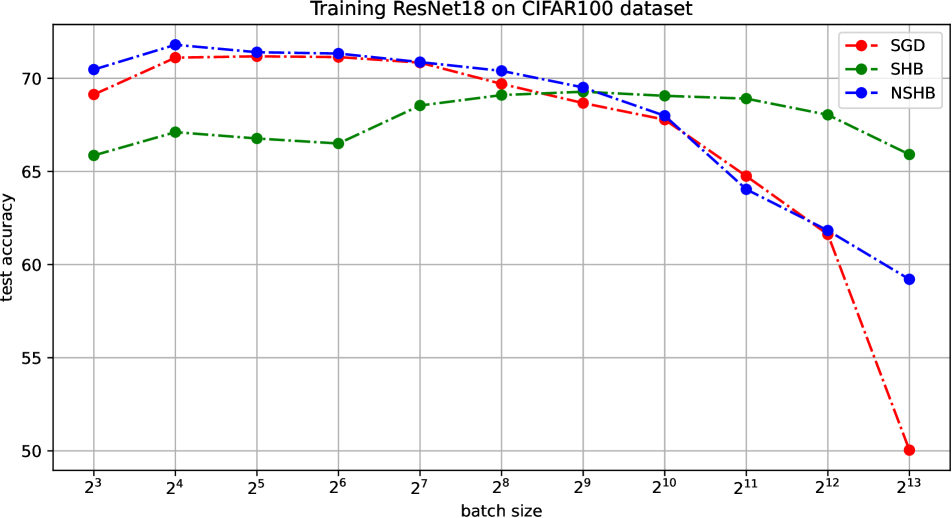
Figure 4: Test accuracy for SGD, SHB, and NSHB versus batch size in training ResNet18 on CIFAR100 dataset.

Implicit graduated optimization with SHB. To test the ability of Algorithm 3 to reduce stochastic noise, we compared a ”constant” method, in which the learning rate, batch size, and momentum are all constant, with a noise reduction method in which the hyperparameters are updated to reduce the degree of smoothing $\delta^{\text{\rm{SHB}}}$. Figure 5 plots the accuracy in testing and the loss function value in training with SHB versus the number of epochs.

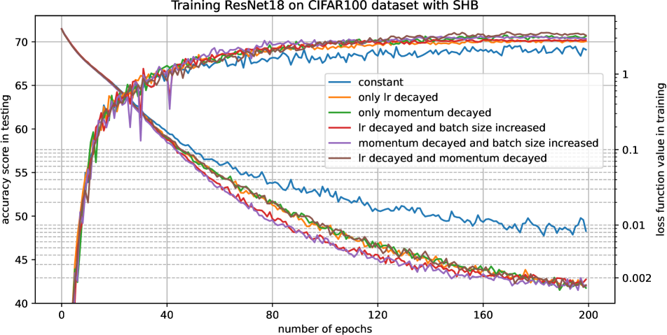
Figure 5: Accuracy score for testing and loss function value for training versus epochs in training of ResNet18 on CIFAR100 dataset with Algorithm 3. ”lr” means the learning rate.

We tuned all noise reduction methods so that the decay rate was $\gamma_{m}:=\frac{(M-m)^{0.9}}{\left\{M-(m-1)\right\}^{0.9}}\ (M=200,m\in[M])$. See Appendix F for the rules for updating the hyperparameters. As shown in Figure 5, the method in which the hyperparameters were updated to reduce the degree of smoothing, i.e., Algorithm 3, outperformed SHB, which used constant parameters, on both test accuracy and loss function value, thereby demonstrating that our algorithm is superior to SGD with momentum with constant parameters on image classification tasks.

5 Conclusion

Our investigation of the smoothing properties of SGD with momentum through convergence analysis and discussion of critical batch size estimation revealed that momentum reduces the variance of the stochastic gradient to less than that of SGD while increasing the degree of smoothing to more than that of SGD. It also showed that the degree of smoothing by SGD with momentum is determined by the learning rate, batch size, and momentum factor, which is larger than that of SGD without momentum, leading to higher generalizability and greater robustness to batch size than SGD. Given these findings, we constructed an implicit graduated optimization algorithm that increases batch size and decreases the momentum factor. Testing demonstrated the superiority of our implicit graduated optimization algorithm on image classification tasks. Our theory that that SGD with momentum smooths the objective function therefore not only resolves inconsistencies regarding the generalizability of momentum but also clarifies the role of hyperparameters. It is thus useful in selecting optimal optimizers and hyperparameters.

Appendix A Convergence analysis of stochastic gradient descent (SGD), stochastic heavy ball (SHB), and quasihyperbolic momentum (QHM)

A.1 Propositions and Lemmas for analyses

Proposition A.1.

For all $\bm{x},\bm{y}\in\mathbb{R}^{d}$ and all $\alpha\in\mathbb{R}$, the following holds:

$$\|\alpha\bm{x}+(1-\alpha)\bm{y}\|^{2}=\alpha\|\bm{x}\|^{2}+(1-\alpha)\|\bm{y}\|^{2}-\alpha(1-\alpha)\|\bm{x}-\bm{y}\|^{2}.$$

Proof.

Since $2\langle\bm{x},\bm{y}\rangle=\|\bm{x}\|^{2}+\|\bm{y}\|^{2}-\|\bm{x}-\bm{y}\|^{2}$ holds, for all $\bm{x},\bm{y}\in\mathbb{R}^{d}$ and all $\alpha\in\mathbb{R}$,

$$\|\alpha\bm{x}+(1-\alpha)\bm{y}\|^{2} =\alpha\|\bm{x}\|^{2}+2\alpha(1-\alpha)\langle\bm{x},\bm{y}\rangle+(1-\alpha)^{2}\|\bm{y}\|^{2}$$

$$=\alpha\|\bm{x}\|^{2}+\alpha(1-\alpha)(\|\bm{x}\|^{2}+\|\bm{y}\|^{2}-\|\bm{x}-\bm{y}\|^{2})+(1-\alpha)^{2}\|\bm{y}\|^{2}$$

$$=\alpha\|\bm{x}\|^{2}+(1-\alpha)\|\bm{y}\|^{2}-\alpha(1-\alpha)\|\bm{x}-\bm{y}\|^{2}.$$

This completes the proof. ∎

Proposition A.2.

For all $\bm{x},\bm{y}\in\mathbb{R}^{d}$, the following holds:

$$\|\bm{x}\pm\bm{y}\|^{2}\leq 2\|\bm{x}\|^{2}+2\|\bm{y}\|^{2}.$$

Proof.

Since $\|\bm{x}\pm\bm{y}\|^{2}=\|\bm{x}\|^{2}\pm 2\langle\bm{x},\bm{y}\rangle+\|\bm{y}\|^{2}$, for all $\bm{x},\bm{y}\in\mathbb{R}^{d}$,

$$\|\bm{x}+\bm{y}\|^{2}+\|\bm{x}-\bm{y}\|^{2}=2\|\bm{x}\|^{2}+2\|\bm{y}\|^{2}.$$

Therefore, we have

$$\|\bm{x}\pm\bm{y}\|^{2} =2\|\bm{x}\|^{2}+2\|\bm{y}\|^{2}-\|\bm{x}\mp\bm{y}\|^{2}$$

$$\leq 2\|\bm{x}\|^{2}+2\|\bm{y}\|^{2}.$$

This completes the proof. ∎

The following proposition describes the relationship between the stationary point problem and variational inequality.

Proposition A.3.

Suppose that $f:\mathbb{R}^{d}\to\mathbb{R}$ is continuously differentiable and $\bm{x}^{*}$ is a stationary point of $f$. Then, $\nabla f(\bm{x}^{*})=\bm{0}$ is equivalent to the following variational inequality: for all $\bm{x}\in\mathbb{R}^{d}$,

$$\langle\nabla f(\bm{x}^{*}),\bm{x}-\bm{x}^{*}\rangle\geq 0.$$

Proof.

Suppose that $\bm{x}\in\mathbb{R}^{d}$ satisfies $\nabla f(\bm{x})=\bm{0}$. Then, for all $\bm{y}\in\mathbb{R}^{d}$,

$$\langle\nabla f(\bm{x}),\bm{y}-\bm{x}\rangle\geq 0.$$

Suppose that $\bm{x}\in\mathbb{R}^{d}$ satisfies $\langle\nabla f(\bm{x}),\bm{y}-\bm{x}\rangle\geq 0$ for all $\bm{y}\in\mathbb{R}^{d}$. Let $\bm{y}:=\bm{x}-\nabla f(\bm{x})$. Then we have

$$0\leq\langle\nabla f(\bm{x}),\bm{y}-\bm{x}\rangle=-\|\nabla f(\bm{x})\|^{2}.$$

Hence,

$$\nabla f(\bm{x})=\bm{0}.$$

This completes the proof. ∎

Lemma A.1.

Suppose that (A2)(ii) and (A3) hold for all $t\in\mathbb{N}$; then,

$$\mathbb{E}_{\bm{\xi}_{t}}\left[\|\nabla f_{\mathcal{S}_{t}}(\bm{x}_{t})-\nabla f(\bm{x}_{t})\|^{2}\right]\leq\frac{C_{\text{\rm{opt}}}^{2}}{b}.$$

Proof.

Let $t\in\mathbb{N}$ and $\bm{\xi}_{t}:=\left(\xi_{t,1},\cdots,\xi_{t,b}\right)^{\top}$. Then, (A2)(ii) and (A3) guarantee that

$$\mathbb{E}_{\bm{\xi}_{t}}\left[\|\nabla f_{\mathcal{S}_{t}}(\bm{x}_{t})-\nabla f(\bm{x}_{t})\|^{2}\big{|}\bm{x}_{t}\right] =\mathbb{E}_{\bm{\xi}_{t}}\left[\left\|\frac{1}{b}\sum_{i=1}^{b}{\mathsf{G}_{\xi_{t,i}}(\bm{x}_{t})}-\nabla f(\bm{x}_{t})\right\|^{2}\right]$$

$$=\mathbb{E}_{\bm{\xi}_{t}}\left[\left\|\frac{1}{b}\sum_{i=1}^{b}{\mathsf{G}_{\xi_{t,i}}(\bm{x}_{t})}-\frac{1}{b}\sum_{i=1}^{b}\nabla f(\bm{x}_{t})\right\|^{2}\right]$$

$$=\mathbb{E}_{\bm{\xi}_{t}}\left[\left\|\frac{1}{b}\sum_{i=1}^{b}\left({\mathsf{G}_{\xi_{t,i}}(\bm{x}_{t})-\nabla f(\bm{x}_{t})}\right)\right\|^{2}\right]$$

$$=\frac{1}{b^{2}}\mathbb{E}_{\bm{\xi}_{t}}\left[\left\|\sum_{i=1}^{b}\left({\mathsf{G}_{\xi_{t,i}}(\bm{x}_{t})-\nabla f(\bm{x}_{t})}\right)\right\|^{2}\right]$$

$$=\frac{1}{b^{2}}\mathbb{E}_{\bm{\xi}_{t}}\left[\sum_{i=1}^{b}\left\|{\mathsf{G}_{\xi_{t,i}}(\bm{x}_{t})-\nabla f(\bm{x}_{t})}\right\|^{2}\right]$$

$$\leq\frac{C_{\text{\rm{opt}}}^{2}}{b}.$$

This completes the proof. ∎

Lemma A.2.

Suppose that Assumptions (A2) and (A4) hold, then for all $t\in\mathbb{N}$,

$$\mathbb{E}\left[\|\nabla f_{\mathcal{S}_{t}}(\bm{x}_{t})\|^{2}\right]\leq\frac{C_{\text{\rm{opt}}}^{2}}{b}+K_{\text{\rm{opt}}}^{2}.$$

Proof.

Let $t\in\mathbb{N}$. From (A2)(i), we obtain

$$\mathbb{E}_{\bm{\xi}_{t}}\left[\|\nabla f_{\mathcal{S}_{t}}(\bm{x}_{t})\|^{2}\big{|}\bm{x}_{t}\right] =\mathbb{E}_{\bm{\xi}_{t}}\left[\|\nabla f_{\mathcal{S}_{t}}(\bm{x}_{t})-\nabla f(\bm{x}_{t})+\nabla f(\bm{x}_{t})\|^{2}\big{|}\bm{x}_{t}\right]$$

$$=\mathbb{E}_{\bm{\xi}_{t}}\left[\|\nabla f_{\mathcal{S}_{t}}(\bm{x}_{t})-\nabla f(\bm{x}_{t})\|^{2}\big{|}\bm{x}_{t}\right]+\mathbb{E}\left[\|\nabla f(\bm{x}_{t})\|^{2}\big{|}\bm{x}_{t}\right]$$

$$\quad+2\mathbb{E}_{\bm{\xi}_{t}}\left[\langle\nabla f_{\mathcal{S}_{t}}(\bm{x}_{t})-\nabla f(\bm{x}_{t}),\nabla f(\bm{x}_{t})\rangle\Big{|}\bm{x}_{t}\right]$$

$$=\mathbb{E}\left[\|\nabla f_{\mathcal{S}_{t}}(\bm{x}_{t})-\nabla f(\bm{x}_{t})\|^{2}\big{|}\bm{x}_{t}\right]+\|\nabla f(\bm{x}_{t})\|^{2},$$

which, together with (A2)(ii), (A4), Lemma A.1, and $\mathbb{E}=\mathbb{E}_{\bm{\xi}_{0}}\mathbb{E}_{\bm{\xi}_{1}}\cdots\mathbb{E}_{\bm{\xi}_{t}}$ implies that

$$\mathbb{E}\left[\|\nabla f_{\mathcal{S}_{t}}(\bm{x}_{t})\|^{2}\right]\leq\frac{C_{\text{\rm{opt}}}^{2}}{b}+K_{\text{\rm{opt}}}^{2}.$$

This completes the proof. ∎

A.2 Lemmas for the convergence analysis of SHB

Lemma A.3.

Suppose that Assumptions (A2)(ii), (A3), and (A4) hold, then for all $t\in\mathbb{N}$,

$$\mathbb{E}\left[\|\bm{m}_{t}\|\right]\leq\frac{1}{1-\beta}\sqrt{\frac{C_{\text{\rm{SHB}}}^{2}}{b}+K_{\text{\rm{SHB}}}^{2}}.$$

Proof.

Let $(\bm{x}_{t})_{t\in\mathbb{N}}$ be the sequence generated by SHB and $t\in\mathbb{N}$. The definition of $\bm{m}_{t}$ implies that

$$\bm{m}_{t} :=\nabla f_{S_{t}}(\bm{x}_{t})+\beta\bm{m}_{t-1}$$

$$=\nabla f_{S_{t}}(\bm{x}_{t})+\beta(\nabla f_{S_{t-1}}(\bm{x}_{t-1})+\beta\bm{m}_{t-2})$$

$$\ \ \vdots$$

$$=\nabla f_{S_{t}}(\bm{x}_{t})+\beta\nabla f_{S_{t-1}}(\bm{x}_{t-1})+\beta^{2}\nabla f_{S_{t-2}}(\bm{x}_{t-2})+\cdots+\beta^{t}\nabla f_{S_{0}}(\bm{x}_{0}).$$

By using the triangle inequality, we obtain

$$\|\bm{m}_{t}\| =\|\nabla f_{S_{t}}(\bm{x}_{t})+\beta\nabla f_{S_{t-1}}(\bm{x}_{t-1})+\beta^{2}\nabla f_{S_{t-2}}(\bm{x}_{t-2})+\cdots+\beta^{t}\nabla f_{S_{0}}(\bm{x}_{0})\|$$

$$\leq\|\nabla f_{S_{t}}(\bm{x}_{t})\|+\beta\|\nabla f_{S_{t-1}}(\bm{x}_{t-1})\|+\beta^{2}\|\nabla f_{S_{t-2}}(\bm{x}_{t-2})\|+\cdots+\beta^{t}\|\nabla f_{S_{0}}(\bm{x}_{0})\|.$$

From Lemma A.2,

$$\mathbb{E}\left[\|\bm{m}_{t}\|\right] \leq\sqrt{\frac{C_{\text{\rm{SHB}}}^{2}}{b}+K_{\text{\rm{SHB}}}^{2}}+\beta\sqrt{\frac{C_{\text{\rm{SHB}}}^{2}}{b}+K_{\text{\rm{SHB}}}^{2}}+\beta^{2}\sqrt{\frac{C_{\text{\rm{SHB}}}^{2}}{b}+K_{\text{\rm{SHB}}}^{2}}+\cdots\beta^{t}\sqrt{\frac{C_{\text{\rm{SHB}}}^{2}}{b}+K_{\text{\rm{SHB}}}^{2}}$$

$$=\frac{(1-\beta^{t})}{1-\beta}\sqrt{\frac{C_{\text{\rm{SHB}}}^{2}}{b}+K_{\text{\rm{SHB}}}^{2}}$$

$$\leq\frac{1}{1-\beta}\sqrt{\frac{C_{\text{\rm{SHB}}}^{2}}{b}+K_{\text{\rm{SHB}}}^{2}}.$$

This completes the proof. ∎

Lemma A.4.

Suppose that Assumptions (A2) and (A4) hold, then for all $t\in\mathbb{N}$,

$$\mathbb{E}\left[\|\bm{m}_{t}\|^{2}\right]\leq\frac{\beta^{2}-\beta+1}{\beta(1-\beta)^{2}}\left(\frac{C_{\text{\rm{SHB}}}^{2}}{b}+K_{\text{\rm{SHB}}}^{2}\right).$$

Proof.

Let $(\bm{x}_{t})_{t\in\mathbb{N}}$ be the sequence generated by SHB and $t\in\mathbb{N}$. Proposition A.1 guarantees that

$$\beta(1-\beta)\|\nabla f_{S_{t}}(\bm{x}_{t})+\bm{m}_{t-1}\|^{2}$$

$$\quad=\beta\|\nabla f_{S_{t}}(\bm{x}_{t-1})\|^{2}+(1-\beta)\|\bm{m}_{t-1}\|^{2}-\|\beta\nabla f_{S_{t}}(\bm{x}_{t})-(1-\beta)\bm{m}_{t-1}\|^{2}$$

$$\quad\leq\beta\|\nabla f_{S_{t}}(\bm{x}_{t})\|^{2}+(1-\beta)\|\bm{m}_{t-1}\|^{2}.$$

Hence,

$$\|\nabla f_{S_{t}}(\bm{x}_{t})+\bm{m}_{t-1}\|^{2}\leq\frac{1}{1-\beta}\|\nabla f_{S_{t}}(\bm{x}_{t})\|^{2}+\frac{1}{\beta}\|\bm{m}_{t-1}\|^{2}.$$ (5)

On the other hand,

$$\|\nabla f_{S_{t}}(\bm{x}_{t})+\bm{m}_{t-1}\|^{2}=\|\nabla f_{S_{t}}(\bm{x}_{t})\|^{2}+2\langle\nabla f_{S_{t}}(\bm{x}_{t}),\bm{m}_{t-1}\rangle+\|\bm{m}_{t-1}\|^{2}.$$ (6)

From (5) and (6), we obtain

$$\|\nabla f_{S_{t}}(\bm{x}_{t})\|^{2}+2\langle\nabla f_{S_{t}}(\bm{x}_{t}),\bm{m}_{t-1}\rangle+\|\bm{m}_{t-1}\|^{2}\leq\frac{1}{1-\beta}\|\nabla f_{S_{t}}(\bm{x}_{t})\|^{2}+\frac{1}{\beta}\|\bm{m}_{t-1}\|^{2}.$$

Therefore,

$$2\langle\nabla f_{S_{t}}(\bm{x}_{t}),\bm{m}_{t-1}\rangle\leq\frac{\beta}{1-\beta}\|\nabla f_{S_{t}}(\bm{x}_{t})\|^{2}+\frac{1-\beta}{\beta}\|\bm{m}_{t-1}\|^{2}.$$ (7)

The definition of $\bm{m}_{t}$ implies that

$$\|\bm{m}_{t}\|^{2} =\|\nabla f_{S_{t}}(\bm{x}_{t})+\beta\bm{m}_{t-1}\|^{2}$$

$$=\|\nabla f_{S_{t}}(\bm{x}_{t})\|^{2}+2\beta\langle\nabla f_{S_{t}}(\bm{x}_{t}),\bm{m}_{t-1}\rangle+\beta^{2}\|\bm{m}_{t-1}\|^{2}.$$ (8)

From (7) and (8), we obtain

$$\|\bm{m}_{t}\|^{2} \leq\frac{\beta^{2}-\beta+1}{1-\beta}\|\nabla f_{S_{t}}(\bm{x}_{t})\|^{2}+\left(\beta^{2}-\beta+1\right)\|\bm{m}_{t-1}\|^{2}$$

$$\leq\frac{\beta^{2}-\beta+1}{1-\beta}\|\nabla f_{S_{t}}(\bm{x}_{t})\|^{2}$$

$$\quad+\left(\beta^{2}-\beta+1\right)\left\{\frac{\beta^{2}-\beta+1}{1-\beta}\|\nabla f_{S_{t-1}}(\bm{x}_{t-1})\|^{2}+\left(\beta^{2}-\beta+1\right)\|\bm{m}_{t-2}\|^{2}\right\}$$

$$\leq\frac{\beta^{2}-\beta+1}{1-\beta}\|\nabla f_{S_{t}}(\bm{x}_{t})\|^{2}+\cdots+\frac{\beta^{2}-\beta+1}{1-\beta}\left(\beta^{2}-\beta+1\right)^{t}\|\nabla f_{S_{0}}(\bm{x}_{0})\|^{2}.$$

By taking the total expectation on both sides, from Lemma A.2, we obtain

$$\mathbb{E}\left[\|\bm{m}_{t}\|^{2}\right] \leq\frac{\beta^{2}-\beta+1}{1-\beta}\mathbb{E}\left[\|\nabla f_{S_{t}}(\bm{x}_{t})\|^{2}\right]+\cdots+\frac{\beta^{2}-\beta+1}{1-\beta}\left(\beta^{2}-\beta+1\right)^{t}\mathbb{E}\left[\|\nabla f_{S_{0}}(\bm{x}_{0})\|^{2}\right]$$

$$\leq\frac{\beta^{2}-\beta+1}{1-\beta}\left(\frac{C_{\text{\rm{SHB}}}^{2}}{b}+K_{\text{\rm{SHB}}}^{2}\right)+\cdots+\frac{\beta^{2}-\beta+1}{1-\beta}\left(\beta^{2}-\beta+1\right)^{t}\left(\frac{C_{\text{\rm{SHB}}}^{2}}{b}+K_{\text{\rm{SHB}}}^{2}\right)$$

$$=\frac{\beta^{2}-\beta+1}{1-\beta}\left(\frac{C_{\text{\rm{SHB}}}^{2}}{b}+K_{\text{\rm{SHB}}}^{2}\right)\cdot\frac{1-\left(\beta^{2}-\beta+1\right)^{t+1}}{1-\left(\beta^{2}-\beta+1\right)}$$

$$\leq\frac{\beta^{2}-\beta+1}{1-\beta}\left(\frac{C_{\text{\rm{SHB}}}^{2}}{b}+K_{\text{\rm{SHB}}}^{2}\right)\cdot\frac{1}{1-\left(\beta^{2}-\beta+1\right)}$$

$$=\frac{\beta^{2}-\beta+1}{1-\beta}\left(\frac{C_{\text{\rm{SHB}}}^{2}}{b}+K_{\text{\rm{SHB}}}^{2}\right)\cdot\frac{1}{\beta(1-\beta)}$$

$$=\frac{\beta^{2}-\beta+1}{\beta(1-\beta)^{2}}\left(\frac{C_{\text{\rm{SHB}}}^{2}}{b}+K_{\text{\rm{SHB}}}^{2}\right).$$

This completes the proof. ∎

A.3 Proof of Theorem 3.1

Proof.

Let $\bm{x}\in\mathbb{R}^{d}$ and $t\in\mathbb{N}$. The definition of $\bm{x}_{t+1}$ implies that

$$\|\bm{x}_{t+1}-\bm{x}\|^{2} =\|(\bm{x}_{t}-\eta\bm{m}_{t})-\bm{x}\|^{2}$$

$$=\|\bm{x}_{t}-\bm{x}\|^{2}-2\eta\langle\bm{x}_{t}-\bm{x},\bm{m}_{t}\rangle+\eta^{2}\|\bm{m}_{t}\|^{2}$$

$$=\|\bm{x}_{t}-\bm{x}\|^{2}-2\eta\langle\bm{x}_{t}-\bm{x},\nabla f_{\mathcal{S}_{t}}(\bm{x}_{t})\rangle+2\eta\beta\langle\bm{x}-\bm{x}_{t},\bm{m}_{t-1}\rangle+\eta^{2}\|\bm{m}_{t}\|^{2}.$$

We then have

$$\mathbb{E}_{\bm{\xi}_{t}}\left[\langle\bm{x}_{t}-\bm{x},\nabla f_{\mathcal{S}_{t}}(\bm{x}_{t})\rangle\Big{|}\bm{x}_{t}\right]=\mathbb{E}_{\bm{\xi}_{t}}\left[\frac{1}{2\eta}\left(\|\bm{x}_{t}-\bm{x}\|^{2}-\|\bm{x}_{t+1}-\bm{x}\|^{2}\right)+\beta\langle\bm{x}-\bm{x}_{t},\bm{m}_{t-1}\rangle+\frac{\eta}{2}\|\bm{m}_{t}\|^{2}\Big{|}\bm{x}_{t}\right].$$

On the other hand, Assumptions (A2)(ii) and (A3) guarantees that

$$\mathbb{E}_{\bm{x}_{t}}\left[\mathbb{E}_{\bm{\xi}_{t}}\left[\left\langle\bm{x}_{t}-\bm{x},\nabla f_{\mathcal{S}_{t}}(\bm{x}_{t})\right\rangle\Big{|}\bm{x}_{t}\right]\right] =\mathbb{E}_{\bm{x}_{t}}\left[\left\langle\bm{x}_{t}-\bm{x},\mathbb{E}_{\bm{\xi}_{t}}\left[\nabla f_{\mathcal{S}_{t}}(\bm{x}_{t})\Big{|}\bm{x}_{t}\right]\right\rangle\right]$$

$$=\mathbb{E}_{\bm{x}_{t}}\left[\langle\bm{x}_{t}-\bm{x},\nabla f(\bm{x}_{t})\rangle\right].$$

Hence, by taking the total expectation on both sides, we obtain

$$\mathbb{E}\left[\langle\bm{x}_{t}-\bm{x},\nabla f(\bm{x}_{t})\rangle\right]=\frac{1}{2\eta}\left(\mathbb{E}\left[\|\bm{x}_{t}-\bm{x}\|^{2}\right]-\mathbb{E}\left[\|\bm{x}_{t+1}-\bm{x}\|^{2}\right]\right)+\beta\mathbb{E}\left[\langle\bm{x}-\bm{x}_{t},\bm{m}_{t-1}\rangle\right]+\frac{\eta}{2}\mathbb{E}\left[\|\bm{m}_{t}\|^{2}\right].$$

According to Lemmas A.3 and A.4, Assumption (S1), and the Cauchy-Schwarz inequality,

$$\mathbb{E}\left[\langle\bm{x}_{t}-\bm{x},\nabla f(\bm{x}_{t})\rangle\right] \leq\frac{1}{2\eta}\left(\mathbb{E}\left[\|\bm{x}_{t}-\bm{x}\|^{2}\right]-\mathbb{E}\left[\|\bm{x}_{t+1}-\bm{x}\|^{2}\right]\right)$$

$$\quad+\frac{\beta D(\bm{x})}{1-\beta}\sqrt{\frac{C_{\text{\rm{SHB}}}^{2}}{b}+K_{\text{\rm{SHB}}}^{2}}+\frac{\eta\left(\beta^{2}-\beta+1\right)}{2\beta(1-\beta)^{2}}\left(\frac{C_{\text{\rm{SHB}}}^{2}}{b}+K_{\text{\rm{SHB}}}^{2}\right).$$

Summing over $t$ from $t=0$ to $t=T-1$, we obtain

$$\sum_{t=0}^{T-1}\mathbb{E}\left[\langle\bm{x}_{t}-\bm{x},\nabla f(\bm{x}_{t})\rangle\right] \leq\frac{1}{2\eta}\left(\mathbb{E}\left[\|\bm{x}_{0}-\bm{x}\|^{2}\right]-\mathbb{E}\left[\|\bm{x}_{T}-\bm{x}\|^{2}\right]\right)$$

$$\quad+\frac{\beta D(\bm{x})}{1-\beta}\sqrt{\frac{C_{\text{\rm{SHB}}}^{2}}{b}+K_{\text{\rm{SHB}}}^{2}}T+\frac{\eta\left(\beta^{2}-\beta+1\right)}{2\beta(1-\beta)^{2}}\left(\frac{C_{\text{\rm{SHB}}}^{2}}{b}+K_{\text{\rm{SHB}}}^{2}\right)T.$$

Therefore,

$$\frac{1}{T}\sum_{t=0}^{T-1}\mathbb{E}\left[\langle\bm{x}_{t}-\bm{x},\nabla f(\bm{x}_{t})\rangle\right]\leq\frac{\|\bm{x}_{0}-\bm{x}\|^{2}}{2\eta T}+\frac{\beta D(\bm{x})}{1-\beta}\sqrt{\frac{C_{\text{\rm{SHB}}}^{2}}{b}+K_{\text{\rm{SHB}}}^{2}}+\frac{\eta\left(\beta^{2}-\beta+1\right)}{2\beta(1-\beta)^{2}}\left(\frac{C_{\text{\rm{SHB}}}^{2}}{b}+K_{\text{\rm{SHB}}}^{2}\right).$$

This completes the proof. ∎

A.4 Lemma for convergence analysis of QHM

Lemma A.5.

Suppose that Assumptions (A2) and (A4) hold, then for all $t\in\mathbb{N}$,

$$\mathbb{E}\left[\|\bm{d}_{t}\|^{2}\right]\leq\frac{C_{\text{\rm{QHM}}}^{2}}{b}+K_{\text{\rm{QHM}}}^{2}.$$

Proof.

The convexity of $\|\cdot\|^{2}$, together with the definition of $\bm{d}_{t}$ and Lemma A.2, guarantees that, for all $t\in\mathbb{N}$,

$$\mathbb{E}\left[\|\bm{d}_{t}\|^{2}\right] \leq\nu\beta\mathbb{E}\left[\|\bm{d}_{t-1}\|^{2}\right]+(1-\nu\beta)\mathbb{E}\left[\|\nabla f_{\mathcal{S}_{t}}(\bm{x}_{t})\|^{2}\right]$$

$$\leq\nu\beta\mathbb{E}\left[\|\bm{d}_{t-1}\|^{2}\right]+(1-\nu\beta)\left(\frac{C_{\text{\rm{QHM}}}^{2}}{b}+K_{\text{\rm{QHM}}}^{2}\right).$$

Induction ensures that, for all $t\in\mathbb{N}$,

$$\mathbb{E}\left[\|\bm{d}_{n}\|^{2}\right]\leq\max\left\{\|\bm{d}_{-1}\|^{2},\frac{C_{\text{\rm{QHM}}}^{2}}{b}+K_{\text{\rm{QHM}}}^{2}\right\}=\frac{C_{\text{\rm{QHM}}}^{2}}{b}+K_{\text{\rm{QHM}}}^{2},$$

where $\bm{d}_{-1}=\bm{0}$. This completes the proof. ∎

A.5 Proof of Theorem 3.2

Proof.

Let $\bm{x}\in\mathbb{R}^{d}$ and $t\in\mathbb{N}$. The definition of $\bm{x}_{t+1}$ implies that

$$\|\bm{x}_{t+1}-\bm{x}\|^{2} =\|(\bm{x}_{t}-\eta\bm{d}_{t})-\bm{x}\|^{2}$$

$$=\|\bm{x}_{t}-\bm{x}\|^{2}-2\eta\langle\bm{x}_{t}-\bm{x},\bm{d}_{t}\rangle+\eta^{2}\|\bm{d}_{t}\|^{2}$$

$$=\|\bm{x}_{t}-\bm{x}\|^{2}-2\eta(1-\nu\beta)\langle\bm{x}_{t}-\bm{x},\nabla f_{\mathcal{S}_{t}}(\bm{x}_{t})\rangle+2\eta\nu\beta\langle\bm{x}-\bm{x}_{t},\bm{d}_{t-1}\rangle+\eta^{2}\|\bm{d}_{t}\|^{2}.$$

Then we have

$$\mathbb{E}_{\bm{\xi}_{t}}\left[\langle\bm{x}_{t}-\bm{x},\nabla f_{\mathcal{S}_{t}}(\bm{x}_{t})\rangle\Big{|}\bm{x}_{t}\right] =\mathbb{E}_{\bm{\xi}_{t}}\left[\frac{1}{2\eta(1-\nu\beta)}\left(\|\bm{x}_{t}-\bm{x}\|^{2}-\|\bm{x}_{t+1}-\bm{x}\|^{2}\right)\right.$$

$$\quad\quad\quad\left.+\frac{\nu\beta}{1-\nu\beta}\langle\bm{x}-\bm{x}_{t},\bm{d}_{t-1}\rangle+\frac{\eta}{2(1-\nu\beta)}\|\bm{d}_{t}\|^{2}\Big{|}\bm{x}_{t}\right].$$

On the other hand, Assumptions (A2)(ii) and (A3) guarantee that

$$\mathbb{E}_{\bm{x}_{t}}\left[\mathbb{E}_{\bm{\xi}_{t}}\left[\left\langle\bm{x}_{t}-\bm{x},\nabla f_{\mathcal{S}_{t}}(\bm{x}_{t})\right\rangle\Big{|}\bm{x}_{t}\right]\right] =\mathbb{E}_{\bm{x}_{t}}\left[\left\langle\bm{x}_{t}-\bm{x},\mathbb{E}_{\bm{\xi}_{t}}\left[\nabla f_{\mathcal{S}_{t}}(\bm{x}_{t})\Big{|}\bm{x}_{t}\right]\right\rangle\right]$$

$$=\mathbb{E}_{\bm{x}_{t}}\left[\langle\bm{x}_{t}-\bm{x},\nabla f(\bm{x}_{t})\rangle\right].$$

Hence, by taking the total expectation on both sides, we obtain

$$\mathbb{E}\left[\langle\bm{x}_{t}-\bm{x},\nabla f(\bm{x}_{t})\rangle\right] =\frac{1}{2\eta(1-\nu\beta)}\left(\mathbb{E}\left[\|\bm{x}_{t}-\bm{x}\|^{2}\right]-\mathbb{E}\left[\|\bm{x}_{t+1}-\bm{x}\|^{2}\right]\right)$$

$$\quad\quad+\frac{\nu\beta}{1-\nu\beta}\mathbb{E}\left[\langle\bm{x}-\bm{x}_{t},\bm{d}_{t-1}\rangle\right]+\frac{\eta}{2(1-\nu\beta)}\mathbb{E}\left[\|\bm{d}_{t}\|^{2}\right].$$

According to Lemma A.5, Assumption (S1), and the Cauchy-Schwarz inequality,

$$\mathbb{E}\left[\langle\bm{x}_{t}-\bm{x},\nabla f(\bm{x}_{t})\rangle\right] \leq\frac{1}{2\eta(1-\nu\beta)}\left(\mathbb{E}\left[\|\bm{x}_{t}-\bm{x}\|^{2}\right]-\mathbb{E}\left[\|\bm{x}_{t+1}-\bm{x}\|^{2}\right]\right)$$

$$\quad+\frac{\nu\beta D(\bm{x})}{1-\nu\beta}\sqrt{\frac{C_{\text{\rm{QHM}}}^{2}}{b}+K_{\text{\rm{QHM}}}^{2}}+\frac{\eta}{2(1-\nu\beta)}\left(\frac{C_{\text{\rm{QHM}}}^{2}}{b}+K_{\text{\rm{QHM}}}^{2}\right).$$

Summing over $t$ from $t=0$ to $t=T-1$, we obtain

$$\sum_{t=0}^{T-1}\mathbb{E}\left[\langle\bm{x}_{t}-\bm{x},\nabla f(\bm{x}_{t})\rangle\right] \leq\frac{1}{2\eta(1-\nu\beta)}\left(\mathbb{E}\left[\|\bm{x}_{0}-\bm{x}\|^{2}\right]-\mathbb{E}\left[\|\bm{x}_{T}-\bm{x}\|^{2}\right]\right)$$

$$\quad+\frac{\nu\beta D(\bm{x})}{1-\nu\beta}\sqrt{\frac{C_{\text{\rm{QHM}}}^{2}}{b}+K_{\text{\rm{QHM}}}^{2}}T+\frac{\eta}{2(1-\nu\beta)}\left(\frac{C_{\text{\rm{QHM}}}^{2}}{b}+K_{\text{\rm{QHM}}}^{2}\right)T.$$

Therefore,

$$\frac{1}{T}\sum_{t=0}^{T-1}\mathbb{E}\left[\langle\bm{x}_{t}-\bm{x},\nabla f(\bm{x}_{t})\rangle\right]\leq\frac{\|\bm{x}_{0}-\bm{x}\|^{2}}{2\eta(1-\nu\beta)T}+\frac{\nu\beta D(\bm{x})}{1-\nu\beta}\sqrt{\frac{C_{\text{\rm{QHM}}}^{2}}{b}+K_{\text{\rm{QHM}}}^{2}}+\frac{\eta}{2(1-\nu\beta)}\left(\frac{C_{\text{\rm{QHM}}}^{2}}{b}+K_{\text{\rm{QHM}}}^{2}\right).$$

This completes the proof. ∎

A.6 Convergence analysis of SGD

convergence analysis of SGD is needed to discuss critical batch size.

Theorem A.1.

Suppose that Assumptions (A1)-(A4) hold and consider the sequence $(\bm{x}_{t})_{t\in\mathbb{N}}$ generated by SGD. Then, for all $\bm{x}\in\mathbb{R}^{d}$ and all $T\geq 1$, the following holds:

$$\frac{1}{T}\sum_{t=0}^{T-1}\mathbb{E}\left[\langle\bm{x}_{t}-\bm{x},\nabla f(\bm{x}_{t})\rangle\right]\leq\frac{\|\bm{x}_{0}-\bm{x}\|^{2}}{2\eta T}+\frac{\eta}{2}\left(\frac{C_{\text{\rm{SGD}}}^{2}}{b}+K_{\text{\rm{SGD}}}^{2}\right).$$

Proof.

Let $\bm{x}\in\mathbb{R}^{d}$ and $t\in\mathbb{N}$. The definition of $\bm{x}_{t+1}$ implies that

$$\|\bm{x}_{t+1}-\bm{x}\|^{2} =\|(\bm{x}_{t}-\eta\nabla f_{\mathcal{S}_{t}}(\bm{x}_{t}))-\bm{x}\|^{2}$$

$$=\|\bm{x}_{t}-\bm{x}\|^{2}-2\eta\langle\bm{x}_{t}-\bm{x},\nabla f_{\mathcal{S}_{t}}(\bm{x}_{t})\rangle+\eta^{2}\|\nabla f_{\mathcal{S}_{t}}(\bm{x}_{t})\|^{2}.$$

Then we have

$$\mathbb{E}_{\bm{\xi}_{t}}\left[\langle\bm{x}_{t}-\bm{x},\nabla f_{\mathcal{S}_{t}}(\bm{x}_{t})\rangle\Big{|}\bm{x}_{t}\right] =\mathbb{E}_{\bm{\xi}_{t}}\left[\frac{1}{2\eta}\left(\|\bm{x}_{t}-\bm{x}\|^{2}-\|\bm{x}_{t+1}-\bm{x}\|^{2}\right)+\frac{\eta}{2}\|\nabla f_{\mathcal{S}_{t}}(\bm{x}_{t}))\|^{2}\Big{|}\bm{x}_{t}\right].$$

On the other hand, Assumptions (A2)(ii) and (A3) guarantee that

$$\mathbb{E}_{\bm{x}_{t}}\left[\mathbb{E}_{\bm{\xi}_{t}}\left[\left\langle\bm{x}_{t}-\bm{x},\nabla f_{\mathcal{S}_{t}}(\bm{x}_{t})\right\rangle\Big{|}\bm{x}_{t}\right]\right] =\mathbb{E}_{\bm{x}_{t}}\left[\left\langle\bm{x}_{t}-\bm{x},\mathbb{E}_{\bm{\xi}_{t}}\left[\nabla f_{\mathcal{S}_{t}}(\bm{x}_{t})\Big{|}\bm{x}_{t}\right]\right\rangle\right]$$

$$=\mathbb{E}_{\bm{x}_{t}}\left[\langle\bm{x}_{t}-\bm{x},\nabla f(\bm{x}_{t})\rangle\right].$$

Hence, by taking the total expectation on both sides, we obtain

$$\mathbb{E}\left[\langle\bm{x}_{t}-\bm{x},\nabla f(\bm{x}_{t})\rangle\right] =\frac{1}{2\eta}\left(\mathbb{E}\left[\|\bm{x}_{t}-\bm{x}\|^{2}\right]-\mathbb{E}\left[\|\bm{x}_{t+1}-\bm{x}\|^{2}\right]\right)+\frac{\eta}{2}\mathbb{E}\left[\|\nabla f_{\mathcal{S}_{t}}(\bm{x}_{t})\|^{2}\right].$$

According to Lemma A.2,

$$\mathbb{E}\left[\langle\bm{x}_{t}-\bm{x},\nabla f(\bm{x}_{t})\rangle\right] \leq\frac{1}{2\eta}\left(\mathbb{E}\left[\|\bm{x}_{t}-\bm{x}\|^{2}\right]-\mathbb{E}\left[\|\bm{x}_{t+1}-\bm{x}\|^{2}\right]\right)+\frac{\eta}{2}\left(\frac{C_{\text{\rm{SGD}}}^{2}}{b}+K_{\text{\rm{SGD}}}^{2}\right).$$

Summing over $t$ from $t=0$ to $t=T-1$, we obtain

$$\sum_{t=0}^{T-1}\mathbb{E}\left[\langle\bm{x}_{t}-\bm{x},\nabla f(\bm{x}_{t})\rangle\right] \leq\frac{1}{2\eta}\left(\mathbb{E}\left[\|\bm{x}_{0}-\bm{x}\|^{2}\right]-\mathbb{E}\left[\|\bm{x}_{T}-\bm{x}\|^{2}\right]\right)+\frac{\eta}{2}\left(\frac{C_{\text{\rm{SGD}}}^{2}}{b}+K_{\text{\rm{SGD}}}^{2}\right)T$$

Therefore,

$$\frac{1}{T}\sum_{t=0}^{T-1}\mathbb{E}\left[\langle\bm{x}_{t}-\bm{x},\nabla f(\bm{x}_{t})\rangle\right]\leq\frac{\|\bm{x}_{0}-\bm{x}\|^{2}}{2\eta T}+\frac{\eta}{2}\left(\frac{C_{\text{\rm{SGD}}}^{2}}{b}+K_{\text{\rm{SGD}}}^{2}\right).$$

This completes the proof. ∎

Appendix B Analysis of critical batch size for SGD, SHB, and QHM

Following earlier studies [26, 52], we derive Proposition 3.1 for estimating a lower bound on the critical batch size. First, the convergence of the optimizer must be analyzed (Theorems A.1, 3.1, and 3.2), and on the basis of that analysis, the number of steps $T$ required for training is defined as a function of batch size $b$ (Theorem B.1). Next, computational complexity is expressed as the number of steps multiplied by the batch size, and computational complexity $T(b)b$ is defined as a function of batch size $b$. Finally, we identify critical batch size $b^{\star}$ that minimizes computational complexity function $T(b)b$ (Theorem B.2) and transform the lower bound for each optimizer (Proposition 3.1).

B.1 Relationship between batch size and number of steps needed for $\epsilon$-approximation

According to Theorems A.1, 3.1, and 3.2, the following hold:

(i) for SGD,

$$\frac{1}{T}\sum_{t=0}^{T-1}\mathbb{E}\left[\langle\bm{x}_{t}-\bm{x},\nabla f(\bm{x}_{t})\rangle\right] \leq\frac{\|\bm{x}_{0}-\bm{x}\|^{2}}{2\eta T}+\frac{\eta}{2}\left(\frac{C_{\text{\rm{SGD}}}^{2}}{b}+K_{\text{\rm{SGD}}}^{2}\right)$$

$$=\underbrace{\frac{\|\bm{x}_{0}-\bm{x}\|^{2}}{2\eta}}_{=:X_{\text{SGD}}}\frac{1}{T}+\underbrace{\frac{\eta C_{\text{SGD}}^{2}}{2}}_{=:Y_{\text{\rm{SGD}}}}\frac{1}{b}+\underbrace{\frac{\eta K_{\text{\rm{SGD}}}^{2}}{2}}_{=:Z_{\text{\rm{SGD}}}};$$ (9)

(ii) for SHB,

$$\frac{1}{T}\sum_{t=0}^{T-1}\mathbb{E}\left[\langle\bm{x}_{t}-\bm{x},\nabla f(\bm{x}_{t})\rangle\right]$$

$$\quad\leq\frac{\|\bm{x}_{0}-\bm{x}\|^{2}}{2\eta T}+\frac{\beta D(\bm{x})}{1-\beta}\sqrt{C_{\text{\rm{SHB}}}^{2}+K_{\text{\rm{SHB}}}^{2}}+\frac{\eta\left(\beta^{2}-\beta+1\right)}{2\beta(1-\beta)^{2}}\left(\frac{C_{\text{\rm{SHB}}}^{2}}{b}+K_{\text{\rm{SHB}}}^{2}\right)$$

$$\quad=\underbrace{\frac{\|\bm{x}_{0}-\bm{x}\|^{2}}{2\eta}}_{=:X_{\text{\rm{SHB}}}}\frac{1}{T}+\underbrace{\frac{\eta\left(\beta^{2}-\beta+1\right)C_{\text{\rm{SHB}}}^{2}}{2\beta(1-\beta)^{2}}}_{=:Y_{\text{\rm{SHB}}}}\frac{1}{b}+\underbrace{\left\{\frac{\eta\left(\beta^{2}-\beta+1\right)}{2\beta(1-\beta)^{2}}K_{\text{\rm{SHB}}}^{2}+\frac{\beta D(\bm{x})}{1-\beta}\sqrt{C_{\text{\rm{SHB}}}^{2}+K_{\text{\rm{SHB}}}^{2}}\right\}}_{=:Z_{\text{\rm{SHB}}}};$$ (10)

(iii) for QHM,

$$\frac{1}{T}\sum_{t=0}^{T-1}\mathbb{E}\left[\langle\bm{x}_{t}-\bm{x},\nabla f(\bm{x}_{t})\rangle\right]$$

$$\quad\leq\frac{\|\bm{x}_{0}-\bm{x}\|^{2}}{2\eta(1-\nu\beta)T}+\frac{\nu\beta D(\bm{x})}{1-\nu\beta}\sqrt{C_{\text{\rm{QHM}}}^{2}+K_{\text{\rm{QHM}}}^{2}}+\frac{\eta}{2(1-\nu\beta)}\left(\frac{C_{\text{\rm{QHM}}}^{2}}{b}+K_{\text{\rm{QHM}}}^{2}\right)$$

$$\quad=\underbrace{\frac{\|\bm{x}_{0}-\bm{x}\|^{2}}{2\eta(1-\nu\beta)}}_{=:X_{\text{\rm{QHM}}}}\frac{1}{T}+\underbrace{\frac{\eta C_{\text{\rm{QHM}}}^{2}}{2(1-\nu\beta)}}_{=:Y_{\text{\rm{QHM}}}}\frac{1}{b}+\underbrace{\left\{\frac{\eta C_{\text{\rm{QHM}}}^{2}}{2(1-\nu\beta)}K_{\text{\rm{QHM}}}^{2}+\frac{\nu\beta D(\bm{x})}{1-\nu\beta}\sqrt{C_{\text{\rm{QHM}}}^{2}+K_{\text{\rm{QHM}}}^{2}}\right\}}_{=:Z_{\text{\rm{QHM}}}}.$$ (11)

The relationship between $b$ and number of steps $T_{\text{\rm{SGD}}}$, $T_{\text{\rm{SHB}}}$, and $T_{\text{\rm{QHM}}}$ satisfying an $\epsilon$-approximation is as follows:

Theorem B.1.

Suppose that Assumptions (A1)-(A4), and (S1) hold and consider SGD, SHB, and QHM. Then, $T_{\text{\rm{SGD}}}(b)$, $T_{\text{\rm{SHB}}}(b)$, and $T_{\text{\rm{QHM}}}(b)$ defined by

$$T_{\text{\rm{SGD}}}(b):=\frac{X_{\text{SGD}}b}{(\epsilon^{2}-Z_{\text{\rm{SGD}}})b-Y_{\text{\rm{SGD}}}}\leq T_{\text{\rm{SGD}}}\text{\ \ for \ }b>{\frac{Y_{\text{\rm{SGD}}}}{\epsilon^{2}-Z_{\text{\rm{SGD}}}}},$$ (12)

$$T_{\text{\rm{SHB}}}(b):=\frac{X_{\text{\rm{SHB}}}b}{(\epsilon^{2}-Z_{\text{\rm{SHB}}})b-Y_{\text{\rm{SHB}}}}\leq T_{\text{\rm{SHB}}}\text{\ \ for \ }b>{\frac{Y_{\text{\rm{SHB}}}}{\epsilon^{2}-Z_{\text{\rm{SHB}}}}},$$ (13)

$$T_{\text{\rm{QHM}}}(b):=\frac{X_{\text{\rm{QHM}}}b}{(\epsilon^{2}-Z_{\text{\rm{QHM}}})b-Y_{\text{\rm{QHM}}}}\leq T_{\text{\rm{QHM}}}\text{\ \ for \ }b>{\frac{Y_{\text{\rm{QHM}}}}{\epsilon^{2}-Z_{\text{\rm{QHM}}}}}$$ (14)

satisfy

$$\frac{1}{T_{\text{\rm{SGD}}}}\sum_{t=0}^{T_{\text{\rm{SGD}}}-1}\mathbb{E}\left[\langle\bm{x}_{t}-\bm{x},\nabla f(\bm{x}_{t})\rangle\right]\leq\epsilon^{2},$$

$$\frac{1}{T_{\text{\rm{SHB}}}}\sum_{t=0}^{T_{\text{\rm{SHB}}}-1}\mathbb{E}\left[\langle\bm{x}_{t}-\bm{x},\nabla f(\bm{x}_{t})\rangle\right]\leq\epsilon^{2},$$

$$\frac{1}{T_{\text{\rm{QHM}}}}\sum_{t=0}^{T_{\text{\rm{QHM}}}-1}\mathbb{E}\left[\langle\bm{x}_{t}-\bm{x},\nabla f(\bm{x}_{t})\rangle\right]\leq\epsilon^{2}.$$

In addition, the functions $T_{\text{\rm{SGD}}}(b)$, $T_{\text{\rm{SHB}}}(b)$, and $T_{\text{\rm{QHM}}}(b)$ defined by (12)-(14) are monotone decreasing and convex for $b>{\frac{Y_{\text{\rm{SGD}}}}{\epsilon^{2}-Z_{\text{\rm{SGD}}}}}$, $b>{\frac{Y_{\text{\rm{SHB}}}}{\epsilon^{2}-Z_{\text{\rm{SHB}}}}}$, and $b>{\frac{Y_{\text{\rm{QHM}}}}{\epsilon^{2}-Z_{\text{\rm{QHM}}}}}$.

Proof.

According to (9) and (12), SGD achieves an $\epsilon$-approximation. We have that, for $b>{\frac{Y_{\text{\rm{SGD}}}}{\epsilon^{2}-Z_{\text{\rm{SGD}}}}}$,

$$\frac{\mathrm{d}T_{\text{\rm{SGD}}}(b)}{\mathrm{d}b}=\frac{-X_{\text{SGD}}Y_{\text{\rm{SGD}}}}{\left\{(\epsilon^{2}-Z_{\text{\rm{SGD}}})b-Y_{\text{\rm{SGD}}}\right\}^{2}}\leq 0,$$

$$\frac{\mathrm{d}^{2}T_{\text{\rm{SGD}}}(b)}{\mathrm{d}b^{2}}=\frac{2X_{\text{SGD}}Y_{\text{\rm{SGD}}}(\epsilon^{2}-Z_{\text{\rm{SGD}}})}{\left\{(\epsilon^{2}-Z_{\text{\rm{SGD}}})b-Y_{\text{\rm{SGD}}}\right\}^{3}}\geq 0.$$

Therefore, $T_{\text{\rm{SGD}}}(b)$ is monotone decreasing and convex for $b>{\frac{Y_{\text{\rm{SGD}}}}{\epsilon^{2}-Z_{\text{\rm{SGD}}}}}$. The discussions for SHB and QHM are similar to the one for SGD. This completes the proof. ∎

B.2 Existence of a critical batch size

The critical batch size minimizes the computational complexity for training. Here, we use stochastic first-order oracle (SFO) complexity as a measure of computational complexity. Since the stochastic gradient is computed $b$ times per step, SFO complexity is defined as

$$T_{\text{\rm{SGD}}}(b)b=\frac{X_{\text{SGD}}b^{2}}{(\epsilon^{2}-Z_{\text{\rm{SGD}}})b-Y_{\text{\rm{SGD}}}},T_{\text{\rm{SHB}}}(b)b=\frac{X_{\text{\rm{SHB}}}b^{2}}{(\epsilon^{2}-Z_{\text{\rm{SHB}}})b-Y_{\text{\rm{SHB}}}},\text{\ and\ \ }T_{\text{\rm{QHM}}}(b)b=\frac{X_{\text{\rm{QHM}}}b^{2}}{(\epsilon^{2}-Z_{\text{\rm{QHM}}})b-Y_{\text{\rm{QHM}}}}.$$ (15)

The following theorem guarantees the existence of critical batch sizes that are global minimizers of $T_{\text{\rm{SGD}}}(b)b$, $T_{\text{\rm{SHB}}}(b)b$, and $T_{\text{\rm{QHM}}}(b)b$ defined by (15).

Theorem B.2.

Suppose that Assumptions (A1)-(A4) and (S1) hold and consider SGD, SHB, and QHM. Then, there exist

$$b_{\text{\rm{SGD}}}^{\star}:=\frac{2Y_{\text{\rm{SGD}}}}{\epsilon^{2}-Z_{\text{\rm{SGD}}}},b_{\text{\rm{SHB}}}^{\star}:=\frac{2Y_{\text{\rm{SHB}}}}{\epsilon^{2}-Z_{\text{\rm{SHB}}}},\text{\ and \ }b_{\text{\rm{QHM}}}^{\star}:=\frac{2Y_{\text{\rm{QHM}}}}{\epsilon^{2}-Z_{\text{\rm{QHM}}}}$$ (16)

such that $b_{\text{\rm{SGD}}}^{\star}$ minimizes the convex function $T_{\text{\rm{SGD}}}(b)b\ (b>Y_{\text{\rm{SGD}}}/(\epsilon^{2}-Z_{\text{\rm{SGD}}}))$, $b_{\text{\rm{SHB}}}^{\star}$ minimizes the convex function $T_{\text{\rm{SHB}}}(b)b\ (b>Y_{\text{\rm{SHB}}}/(\epsilon^{2}-Z_{\text{\rm{SHB}}}))$, and $b_{\text{\rm{QHM}}}^{\star}$ minimizes the convex function $T_{\text{\rm{QHM}}}(b)b\ (b>Y_{\text{\rm{QHM}}}/(\epsilon^{2}-Z_{\text{\rm{QHM}}}))$.

Proof.

From (16), we have that, for $b>Y_{\text{\rm{SGD}}}/(\epsilon^{2}-Z_{\text{\rm{SGD}}}))$,

$$\frac{\mathrm{d}T_{\text{\rm{SGD}}}(b)b}{\mathrm{d}b}=\frac{X_{\text{SGD}}b\left\{(\epsilon^{2}-Z_{\text{\rm{SGD}}})b-2Y_{\text{\rm{SGD}}}\right\}}{\left\{(\epsilon^{2}-Z_{\text{\rm{SGD}}})b-Y_{\text{\rm{SGD}}}\right\}^{2}},$$

$$\frac{\mathrm{d}^{2}T_{\text{\rm{SGD}}}(b)b}{\mathrm{d}b^{2}}=\frac{2X_{\text{SGD}}Y_{\text{\rm{SGD}}}^{2}}{\left\{(\epsilon^{2}-Z_{\text{\rm{SGD}}})b-Y_{\text{\rm{SGD}}}\right\}^{3}}\geq 0.$$

Hence, $T_{\text{\rm{SGD}}}(b)b$ is convex for $b>Y_{\text{\rm{SGD}}}/(\epsilon^{2}-Z_{\text{\rm{SGD}}})$ and

$$\frac{\mathrm{d}T_{\text{\rm{SGD}}}(b)b}{\mathrm{d}b}\begin{cases}<0&\text{ if }b<b_{\text{\rm{SGD}}}^{\star},\\ =0&\text{ if }b=b_{\text{\rm{SGD}}}^{\star}=\frac{2Y_{\text{\rm{SGD}}}}{\epsilon^{2}-Z_{\text{\rm{SGD}}}},\\ >0&\text{ if }b>b_{\text{\rm{SGD}}}^{\star}.\end{cases}$$

The discussions for SHB and QHM are similar to the one for SGD. This completes the proof. ∎

B.3 Proof of Proposition 3.1

Proof.

Theorem B.2 and the definition of $Y_{\text{\rm{SGD}}}$ and $Z_{\text{\rm{SGD}}}$ (see (9)) ensure that

$$b_{\text{\rm{SGD}}}^{\star}:=\frac{2Y_{\text{\rm{SGD}}}}{\epsilon^{2}-Z_{\text{\rm{SGD}}}}>\frac{2Y_{\text{\rm{SGD}}}}{\epsilon^{2}}=\frac{2}{\epsilon^{2}}\cdot\frac{\eta C_{\text{\rm{SGD}}}^{2}}{2}=\frac{\eta C_{\text{\rm{SGD}}}^{2}}{\epsilon^{2}}.$$

Similarly, for SHB, from Theorem B.2 and the definition of $Y_{\text{\rm{SHB}}}$ and $Z_{\text{\rm{SHB}}}$ (see (10)), we obtain

$$b_{\text{\rm{SHB}}}^{\star}:=\frac{2Y_{\text{\rm{SHB}}}}{\epsilon^{2}-Z_{\text{\rm{SHB}}}}>\frac{2Y_{\text{\rm{SHB}}}}{\epsilon^{2}}=\frac{2}{\epsilon^{2}}\cdot\frac{\eta\left(\beta^{2}-\beta+1\right)C_{\text{\rm{SHB}}}^{2}}{2\beta(1-\beta)^{2}}=\frac{\eta\left(\beta^{2}-\beta+1\right)C_{\text{\rm{SHB}}}^{2}}{\beta(1-\beta)^{2}\epsilon^{2}}.$$

Finally, for QHM, from Theorem B.2 and the definition of $Y_{\text{\rm{QHM}}}$ and $Z_{\text{\rm{QHM}}}$ (see (11)), we obtain

$$b_{\text{\rm{QHM}}}^{\star}:=\frac{2Y_{\text{\rm{QHM}}}}{\epsilon^{2}-Z_{\text{\rm{QHM}}}}>\frac{2Y_{\text{\rm{QHM}}}}{\epsilon^{2}}=\frac{2}{\epsilon^{2}}\cdot\frac{\eta C_{\text{\rm{QHM}}}^{2}}{2(1-\nu\beta)}=\frac{\eta C_{\text{\rm{QHM}}}^{2}}{(1-\nu\beta)\epsilon^{2}}.$$

This completes the proof. ∎

B.4 More details on experimental results in Section 3.3

Since SFO complexity is expressed as the product of the number of steps and the batch size, we first measured the number of steps $T$ required to achieve a sufficiently small gradient norm for each batch size. Figure 7 plots the number of steps $T$ needed to achieve the gradient norm of the past $t$ steps at time $t$ to average less than $\epsilon=0.5$ versus batch size $b$. The figure shows that the number of steps for each optimizer was mostly monotone decreasing and convex with respect to batch size $b$, which provides experimental support for Theorem B.1. Next, we calculated SFO complexity by multiplying number of steps $T$ by batch size $b$. As shown in Figure 7, SFO complexity for each optimizer was convex with respect to batch size $b$, which provides experimental support for Theorem B.2. We performed similar experiments on training WideResNet-28-10 on CIFAR100 and obtained similar results. The results are plotted in Figures 9 and 9.

B.5 Computing variance of stochastic gradient using Proposition 3.1

From Proposition 3.1 and the hyperparameters used in the experiments for training ResNet18 on the CIFAR100 dataset, we obtained

$$C_{\text{\rm{SGD}}}^{2}<\frac{b_{\text{\rm{SGD}}}^{\star}\epsilon^{2}}{\eta}=\frac{2^{9}\cdot(0.5)^{2}}{0.1}=1280,$$

$$C_{\text{\rm{SHB}}}^{2}<\frac{b_{\text{\rm{SHB}}}^{\star}\epsilon^{2}\beta(1-\beta)^{2}}{\eta(\beta^{2}-\beta+1)}=\frac{2^{10}\cdot(0.5)^{2}\cdot 0.9\cdot(0.1)^{2}}{0.1\cdot 0.91}=25.318,$$

$$C_{\text{\rm{NSHB}}}^{2}<\frac{b_{\text{\rm{NSHB}}}^{\star}\epsilon^{2}(1-\nu\beta)}{\eta}=\frac{2^{9}\cdot(0.5)^{2}\cdot(1-1\cdot 0.9)}{0.1}=128,$$

where $\eta=0.1,\beta=0.9,\nu=1$, and $\epsilon=0.5$ were used in the experiments and $b_{\text{\rm{SGD}}}^{\star}=2^{9},b_{\text{\rm{SHB}}}^{\star}=2^{10}$, and $b_{\text{\rm{NSHB}}}^{\star}=2^{9}$ were measured by experiment (see Figure 7).

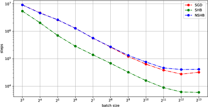
Figure 6: Number of steps for SGD, SHB, and NSHB needed to train ResNet18 on CIFAR100 dataset versus batch size.

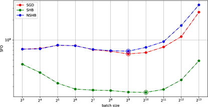
Figure 7: SFO complexities for SGD, SHB, and NSHB needed to train ResNet18 on CIFAR100 dataset versus batch size. The double circle denotes the critical batch size that minimizes SFO complexity. This is the same graph shown in Figure 2.

From a similar discussion, for training WideResNet-28-10 on the CIFAR100 dataset, we obtained

$$C_{\text{\rm{SGD}}}^{2}<\frac{b_{\text{\rm{SGD}}}^{\star}\epsilon^{2}}{\eta}=\frac{2^{2}\cdot(0.5)^{2}}{0.1}=10,$$

$$C_{\text{\rm{SHB}}}^{2}<\frac{b_{\text{\rm{SHB}}}^{\star}\epsilon^{2}\beta(1-\beta)^{2}}{\eta(\beta^{2}-\beta+1)}=\frac{2^{5}\cdot(0.5)^{2}\cdot 0.9\cdot(0.1)^{2}}{0.1\cdot 0.91}=0.79,$$

$$C_{\text{\rm{NSHB}}}^{2}<\frac{b_{\text{\rm{NSHB}}}^{\star}\epsilon^{2}(1-\nu\beta)}{\eta}=\frac{2^{2}\cdot(0.5)^{2}\cdot(1-1\cdot 0.9)}{0.1}=1.0,$$

where $\eta=0.1,\beta=0.9,\nu=1$, and $\epsilon=0.5$ were used in the experiments and $b_{\text{\rm{SGD}}}^{\star}=2^{2},b_{\text{\rm{SHB}}}^{\star}=2^{5}$, and $b_{\text{\rm{NSHB}}}^{\star}=2^{2}$ were measured by experiment (see Figure 9).

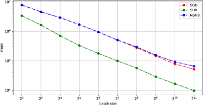
Figure 8: Number of steps for SGD, SHB, and NSHB needed to train WideResNet-28-10 on CIFAR100 dataset versus batch size.

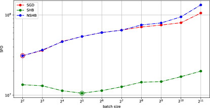
Figure 9: SFO complexities for SGD, SHB, and NSHB needed to train WideResNet-28-10 on CIFAR100 dataset versus batch size. The double circle denotes the critical batch size that minimizes SFO complexity.

To discuss the noise level of smoothing in Section 4.1, we also measured the gradient norm and its upper bound. The measured gradient norm was larger for smaller batch sizes, with maximum values of $4.528$, $1.77$, and $4.5$ for SGD, SHB, and NSHB, respectively. We used this value as an upper bound on the gradient norm (i.e., $K_{\text{\rm{SGD}}}:=4.528$, $K_{\text{\rm{SHB}}}:=1.77$, and $K_{\text{\rm{NSHB}}}:=4.5$) for training ResNet18 on the CIFAR100 dataset. We also used it as an upper bound on the gradient norm ($K_{\text{\rm{SGD}}}:=4.259$, $K_{\text{\rm{SHB}}}:=1.66$, and $K_{\text{\rm{NSHB}}}:=4.262$) for training WideResNet-28-10 on the CIFAR100 dataset.

Appendix C Smoothing property of optimizers with a mini-batch stochastic gradient

C.1 Proof of Proposition 4.1

Proof.

The definition of $\bm{m}_{t}$ implies that

$$\left\|\bm{\omega}_{t}^{\text{\rm{SHB}}}\right\|^{2} =\|\bm{m}_{t}-\nabla f(\bm{x}_{t})\|^{2}$$

$$=\|\nabla f_{\mathcal{S}_{t}}(\bm{x}_{t})+\beta\bm{m}_{t-1}-\nabla f(\bm{x}_{t})\|^{2}$$

$$=\|\nabla f_{\mathcal{S}_{t}}(\bm{x}_{t})-\nabla f(\bm{x}_{t})\|^{2}+2\beta\langle\nabla f_{\mathcal{S}_{t}}(\bm{x}_{t})-\nabla f(\bm{x}_{t}),\bm{m}_{t-1}\rangle+\beta^{2}\|\bm{m}_{t-1}\|^{2}.$$

Hence, from Lemmas A.2 and A.4, we obtain

$$\mathbb{E}\left[\left\|\bm{\omega}_{t}^{\text{\rm{SHB}}}\right\|^{2}\right] =\mathbb{E}\left[\|\nabla f_{\mathcal{S}_{t}}(\bm{x}_{t})-\nabla f(\bm{x}_{t})\|^{2}\right]+\beta^{2}\mathbb{E}\left[\|\bm{m}_{t-1}\|^{2}\right]$$

$$\leq\frac{C_{\text{\rm{SHB}}}^{2}}{b}+\frac{\beta(\beta^{2}-\beta+1)}{(1-\beta)^{2}}\left(\frac{C_{\text{\rm{SHB}}}^{2}}{b}+K_{\text{\rm{SHB}}}^{2}\right)$$

$$=\left(1+\frac{\beta(\beta^{2}-\beta+1)}{(1-\beta)^{2}}\right)\frac{C_{\text{\rm{SHB}}}^{2}}{b}+\frac{\beta(\beta^{2}-\beta+1)}{(1-\beta)^{2}}K_{\text{\rm{SHB}}}^{2}.$$

Similarly, the definition of $\bm{d}_{t}$ implies that

$$\left\|\bm{\omega}_{t}^{\text{\rm{QHM}}}\right\|^{2} =\|\bm{d}_{t}-\nabla f(\bm{x}_{t})\|^{2}$$

$$=\|(1-\nu\beta)\nabla f_{\mathcal{S}_{t}}(\bm{x}_{t})+\nu\beta\bm{d}_{t-1}-\nabla f(\bm{x}_{t})\|^{2}$$

$$=\|\nabla f_{\mathcal{S}_{t}}(\bm{x}_{t})-\nabla f(\bm{x}_{t})+\nu\beta(\bm{d}_{t-1}-\nabla f_{\mathcal{S}_{t}}(\bm{x}_{t}))\|^{2}$$

$$=\|\nabla f_{\mathcal{S}_{t}}(\bm{x}_{t})-\nabla f(\bm{x}_{t})\|^{2}+2\nu\beta\langle\nabla f_{\mathcal{S}_{t}}(\bm{x}_{t})-\nabla f(\bm{x}_{t}),\bm{d}_{t-1}-\nabla f_{\mathcal{S}_{t}}(\bm{x}_{t})\rangle+\nu^{2}\beta^{2}\|\bm{d}_{t-1}-\nabla f_{\mathcal{S}_{t}}(\bm{x}_{t})\|^{2}.$$

Therefore, from Proposition A.2, Lemmas A.1, A.2, and A.5, we obtain

$$\mathbb{E}\left[\left\|\bm{\omega}_{t}^{\text{\rm{QHM}}}\right\|^{2}\right] =\mathbb{E}\left[\|\nabla f_{\mathcal{S}_{t}}(\bm{x}_{t})-\nabla f(\bm{x}_{t})\|^{2}\right]+\nu^{2}\beta^{2}\mathbb{E}\left[\|\bm{d}_{t-1}-\nabla f_{\mathcal{S}_{t}}(\bm{x}_{t})\|^{2}\right]$$

$$\leq\mathbb{E}\left[\|\nabla f_{\mathcal{S}_{t}}(\bm{x}_{t})-\nabla f(\bm{x}_{t})\|^{2}\right]+\nu^{2}\beta^{2}\left(2\mathbb{E}\left[\|\bm{d}_{t-1}\|^{2}\right]+2\mathbb{E}\left[\|\nabla f_{\mathcal{S}_{t}}(\bm{x}_{t})\|^{2}\right]\right)$$

$$\leq\frac{C_{\text{\rm{QHM}}}^{2}}{b}+\nu^{2}\beta^{2}\left\{2\left(\frac{C_{\text{\rm{QHM}}}^{2}}{b}+K_{\text{\rm{QHM}}}^{2}\right)+2\left(\frac{C_{\text{\rm{QHM}}}^{2}}{b}+K_{\text{\rm{QHM}}}^{2}\right)\right\}$$

$$=\left(1+4\nu^{2}\beta^{2}\right)\frac{C_{\text{\rm{QHM}}}^{2}}{b}+4\nu^{2}\beta^{2}K_{\text{\rm{QHM}}}^{2}.$$

This completes the proof. ∎

C.2 Derivation of equation (1)

Let $\bm{y}_{t}$ be the parameter updated by the gradient descent and $\bm{x}_{t+1}$ be the parameter updated by SHB at time $t$; i.e.,

$$\bm{y}_{t} :=\bm{x}_{t}-\eta\nabla f(\bm{x}_{t}),$$

$$\bm{x}_{t+1} :=\bm{x}_{t}-\eta\bm{m}_{t}$$

$$=\bm{x}_{t}-\eta(\nabla f(\bm{x}_{t})+\bm{\omega}_{t}^{\text{\rm{SHB}}}).$$

Then, we obtain

$$\bm{x}_{t+1} :=\bm{x}_{t}-\eta\bm{m}_{t}$$

$$=\left(\bm{y}_{t}+\eta\nabla f(\bm{x}_{t})\right)-\eta\bm{m}_{t}$$

$$=\bm{y}_{t}-\eta\bm{\omega}_{t}^{\text{\rm{SHB}}},$$ (17)

from $\bm{\omega}_{t}^{\text{\rm{SHB}}}:=\bm{m}_{t}-\nabla f(\bm{x}_{t})$. Hence,

$$\bm{y}_{t+1} =\bm{x}_{t+1}-\eta\nabla f(\bm{x}_{t+1})$$

$$=\bm{y}_{t}-\eta\bm{\omega}_{t}^{\text{\rm{SHB}}}-\eta\nabla f(\bm{y}_{t}-\eta\bm{\omega}_{t}^{\text{\rm{SHB}}}).$$

By taking the expectation with respect to $\bm{\omega}_{t}^{\text{\rm{SHB}}}$ on both sides, we obtain, from $\mathbb{E}_{\bm{\omega}_{t}^{\text{\rm{SHB}}}}\left[\bm{\omega}_{t}^{\text{\rm{SHB}}}\right]=\bm{0}$,

$$\mathbb{E}_{\bm{\omega}_{t}^{\text{\rm{SHB}}}}\left[\bm{y}_{t+1}\right]=\bm{y}_{t}-\eta\nabla\mathbb{E}_{\bm{\omega}_{t}^{\text{\rm{SHB}}}}\left[f(\bm{y}_{t}-\eta\bm{\omega}_{t}^{\text{\rm{SHB}}})\right].$$

In addition, from (17) and $\mathbb{E}_{\bm{\omega}_{t}^{\text{\rm{SHB}}}}\left[\bm{\omega}_{t}^{\text{\rm{SHB}}}\right]=\bm{0}$, we obtain

$$\mathbb{E}_{\bm{\omega}_{t}^{\text{\rm{SHB}}}}\left[\bm{x}_{t+1}\right]=\bm{y}_{t}.$$

Therefore, on average, parameter $\bm{x}_{t+1}$ of function $f$ arrived at using the SHB method coincides with parameter $\bm{y}_{t}$ of smoothed function $\hat{f}(\bm{y}_{t}):=\mathbb{E}_{\bm{\omega}_{t}^{\text{\rm{SHB}}}}\left[f(\bm{y}_{t}-\eta\bm{\omega}_{t}^{\text{\rm{SHB}}})\right]$ arrived at using gradient descent. A similar discussion yields a similar equation for QHM.

C.3 Details of calculating degree of smoothing in Figure 3

From (2)-(4), the hyperparameters used in the experiments, and the value estimated in Section 3.3 for training ResNet18 on the CIFAR100 dataset, the degree of smoothing can be calculated as

$$\delta^{\text{\rm{SGD}}}=\eta\sqrt{\frac{C_{\text{\rm{SGD}}}^{2}}{b}}=0.1\cdot\sqrt{\frac{1280}{b}}=\sqrt{\frac{12.8}{b}},$$

$$\delta^{\text{\rm{SHB}}}=\eta\sqrt{\frac{C_{\text{\rm{SHB}}}^{2}}{b}+\frac{\beta(\beta^{2}-\beta+1)}{(1-\beta)^{2}}\left(\frac{C_{\text{\rm{SHB}}}^{2}}{b}+K_{\text{\rm{SHB}}}^{2}\right)} =0.1\cdot\sqrt{\frac{25.318}{b}+\frac{0.9\cdot 0.91}{(0.1)^{2}}\left(\frac{25.318}{b}+(1.77)^{2}\right)}$$

$$=0.1\cdot\sqrt{82.9\cdot\frac{25.318}{b}+81.9\cdot 3.1329}$$

$$\approx\sqrt{\frac{21}{b}+2.57},$$

$$\delta^{\text{\rm{NSHB}}}=\eta\sqrt{\frac{C_{\text{\rm{NSHB}}}^{2}}{b}+4\beta^{2}\left(\frac{C_{\text{\rm{NSHB}}}^{2}}{b}+K_{\text{\rm{NSHB}}}^{2}\right)} =0.1\cdot\sqrt{\frac{128}{b}+4\cdot(0.9)^{2}\cdot\left(\frac{128}{b}+(4.5)^{2}\right)}$$

$$=0.1\cdot\sqrt{4.24\cdot\frac{128}{b}+3.24\cdot 20.25}$$

$$\approx\sqrt{\frac{5.4}{b}+0.66},$$

where $\eta=0.1$ and $\beta=0.9$ were used in the experiments, $C_{\text{\rm{SGD}}}^{2}=1280,C_{\text{\rm{SHB}}}^{2}=25.318$, and $C_{\text{\rm{NSHB}}}^{2}=128$ were calculated in Section 3.3, and $K_{\text{\rm{SHB}}}:=1.77$ and $K_{\text{\rm{NSHB}}}:=4.5$ were observed in Section B.5. Figure 11 plots the computed degrees of smoothing $\delta^{\text{\rm{SGD}}},\delta^{\text{\rm{SHB}}}$, and $\delta^{\text{\rm{NSHB}}}$ versus batch size $b$ in training ResNet18 on CIFAR100. Figure 11 is a logarithmic graph version of Figure 11.

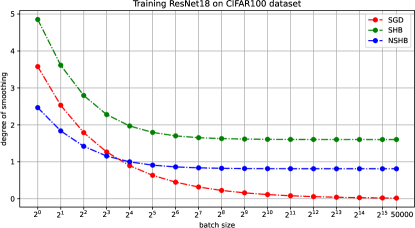
Figure 10: Degrees of smoothing $\delta^{\text{\rm{SGD}}},\delta^{\text{\rm{SHB}}}$, and $\delta^{\text{\rm{NSHB}}}$ versus batch size in training ResNet18 on CIFAR100 dataset. This is the same graph shown in Figure 3.

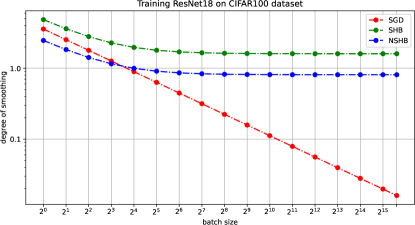
Figure 11: Llogarithmic graph version of Figure 11, clearly showing that $\delta^{\text{\rm{SGD}}}$ becomes smaller as the batch size is increased.

A similar argument can be made for the WideResNet-28-10 training. From (2)-(4), the hyperparameters used in the experiments, and the value estimated in Section 3.3 for training WideResNet-28-10 on the CIFAR100 dataset, the degree of smoothing can be calculated as

$$\delta^{\text{\rm{SGD}}}=\eta\sqrt{\frac{C_{\text{\rm{SGD}}}^{2}}{b}}=0.1\cdot\sqrt{\frac{10}{b}}=\sqrt{\frac{0.1}{b}},$$

$$\delta^{\text{\rm{SHB}}}=\eta\sqrt{\frac{C_{\text{\rm{SHB}}}^{2}}{b}+\frac{\beta(\beta^{2}-\beta+1)}{(1-\beta)^{2}}\left(\frac{C_{\text{\rm{SHB}}}^{2}}{b}+K_{\text{\rm{SHB}}}^{2}\right)} =0.1\cdot\sqrt{\frac{0.79}{b}+\frac{0.9\cdot 0.91}{(0.1)^{2}}\left(\frac{0.79}{b}+(1.66)^{2}\right)}$$

$$=0.1\cdot\sqrt{82.9\cdot\frac{0.79}{b}+81.9\cdot 2.7556}$$

$$\approx\sqrt{\frac{0.65}{b}+2.26},$$

$$\delta^{\text{\rm{NSHB}}}=\eta\sqrt{\frac{C_{\text{\rm{NSHB}}}^{2}}{b}+4\beta^{2}\left(\frac{C_{\text{\rm{NSHB}}}^{2}}{b}+K_{\text{\rm{NSHB}}}^{2}\right)} =0.1\cdot\sqrt{\frac{1}{b}+4\cdot(0.9)^{2}\cdot\left(\frac{1}{b}+(4.262)^{2}\right)}$$

$$=0.1\cdot\sqrt{4.24\cdot\frac{1}{b}+3.24\cdot 18.16}$$

$$\approx\sqrt{\frac{0.04}{b}+0.59},$$

where $\eta=0.1$ and $\beta=0.9$ were used in the experiments, $C_{\text{\rm{SGD}}}^{2}=10,C_{\text{\rm{SHB}}}^{2}=0.79$, and $C_{\text{\rm{NSHB}}}^{2}=1.0$ were calculated in Section 3.3, and $K_{\text{\rm{SHB}}}:=1.66$ and $K_{\text{\rm{NSHB}}}:=4.262$ were observed in Section B.5. Figure 13 plots the computed degrees of smoothing $\delta^{\text{\rm{SGD}}},\delta^{\text{\rm{SHB}}}$, and $\delta^{\text{\rm{NSHB}}}$ versus batch size $b$ in training WideResNet-28-10 on CIFAR100. Figure 13 is a logarithmic graph version of Figure 13 showing that, for WideResNet-28-10 as well, the degree of smoothing with SGD with momentum is always greater than with SGD. A comparison of Figures 11 and 13 shows that each optimizer was more robust to batch size in training WideResNet-28-10 than in training ResNet18. Therefore, generalizability may be less affected by batch size for training WideResNet-28-10 than for training ResNet18. This is shown to be true in Appendix F.1.

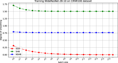
Figure 12: Degrees of smoothing $\delta^{\text{\rm{SGD}}},\delta^{\text{\rm{SHB}}}$, and $\delta^{\text{\rm{NSHB}}}$ versus batch size in training WideResNet-28-10 on CIFAR100 dataset.

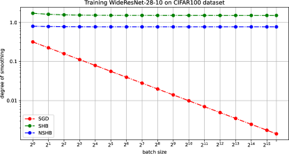
Figure 13: Logarithmic graph version of Figure 13 more clearly showing that $\delta^{\text{\rm{SGD}}}$ becomes smaller as the batch size is increased.

Appendix D Convergence analysis of Algorithm 3

This section provides the proof of Theorem 4.1. The new $\sigma$-nice function admits that each of the smoothed $M$ functions is $\sigma$-strongly convex in neighborhood $N(\bm{x}^{\star};d_{m}|\delta_{m}|)\ (m\in[M])$ (see Definition 4.2). Note that Algorithm 4 can therefore be applied to $\sigma$-strongly convex functions although it does not require the original function $f$ to be $\sigma$-strongly convex. First, we admit the following theorem on the basis of convergence analysis of gradient descent (Algorithm 4) for $\sigma$-strongly convex functions.

D.1 Theorem and Lemmas for the analyses

Theorem D.1 (Convergence analysis of Algorithm 4).

[53, Theorem 3] Suppose that Assumption (A2) holds, where $\mathsf{G}_{\xi_{t}}$ is the stochastic gradient of a $\sigma$-strongly convex and $L_{g}$-smooth function $F\colon\mathbb{R}^{d}\to\mathbb{R}$, and $\eta<\min\left\{\frac{1}{\sigma},\frac{2}{L_{g}}\right\}$. Then, the sequence $(\hat{\bm{x}}_{t})_{t\in\mathbb{N}}$ generated by Algorithm 4 satisfies

$$\min_{t\in[T]}\mathbb{E}\left[F\left(\hat{\bm{x}}_{t}\right)-F(\bm{x}^{\star})\right]\leq\frac{H_{4}}{T}+H_{3}\eta=\mathcal{O}\left(\frac{1}{T}+\eta\right),$$

where $\bm{x}^{\star}$ is the global minimizer of $F$, and $H_{4}\text{ and }H_{3}>0$ are nonnegative constants.

Theorem D.1 shows that Algorithm 4 can reach an $\epsilon_{m}$-neighborhood of optimal solution $\bm{x}_{{\delta}_{m}}^{\star}$ of $\hat{f}_{\delta_{m}}$ in approximately $T_{F}:=\frac{H_{4}}{\epsilon_{m}-H_{3}\eta}$ iterations.

Lemma D.1.

Suppose that (C2) holds; then $\hat{f}_{\delta}$ is an $L_{f}$-Lipschitz function; i.e., for all $\bm{x},\bm{y}\in\mathbb{R}^{d}$,

$$\left|\hat{f}_{\delta}(\bm{x})-\hat{f}_{\delta}(\bm{y})\right|\leq L_{f}\|\bm{x}-\bm{y}\|.$$

Proof.

From Definition 4.1 and (C2), we obtain, for all $\bm{x},\bm{y}\in\mathbb{R}^{d}$,

$$\left|\hat{f}_{\delta}(\bm{x})-\hat{f}_{\delta}(\bm{y})\right| =\left|\mathbb{E}_{\bm{u}}\left[f(\bm{x}-\delta\bm{u})\right]-\mathbb{E}_{\bm{u}}\left[f(\bm{y}-\delta\bm{u})\right]\right|$$

$$=\left|\mathbb{E}_{\bm{u}}\left[f(\bm{x}-\delta\bm{u})-f(\bm{y}-\delta\bm{u})\right]\right|$$

$$\leq\mathbb{E}_{\bm{u}}\left[\left|f(\bm{x}-\delta\bm{u})-f(\bm{y}-\delta\bm{u})\right|\right]$$

$$\leq\mathbb{E}_{\bm{u}}\left[L_{f}\|(\bm{x}-\delta\bm{u})-(\bm{y}-\delta\bm{u})\|\right]$$

$$=\mathbb{E}_{\bm{u}}\left[L_{f}\left\|\bm{x}-\bm{y}\right\|\right]$$

$$=L_{f}\|\bm{x}-\bm{y}\|.$$

This completes the proof. ∎

Lemma D.1 implies that Lipschitz constant $L_{f}$ of original function $f$ is carried over to function $\hat{f}_{\delta}$ smoothed by any $\delta\in\mathbb{R}$.

Lemma D.2.

Let $\hat{f}_{\delta}$ be the smoothed version of $f$; then, for all $\bm{x}\in\mathbb{R}^{d}$,

$$\left|\hat{f}_{\delta}(\bm{x})-f(\bm{x})\right|\leq|\delta|L_{f}.$$

Proof.

From Definition 4.1 and (C2), we have, for all $\bm{x},\bm{y}\in\mathbb{R}^{d}$,

$$\left|\hat{f}_{\delta}(\bm{x})-f(\bm{x})\right| =\left|\mathbb{E}_{\bm{u}}\left[f(\bm{x}-\delta\bm{u})\right]-f(\bm{x})\right|$$

$$=\left|\mathbb{E}_{\bm{u}}\left[f(\bm{x}-\delta\bm{u})-f(\bm{x})\right]\right|$$

$$\leq\mathbb{E}_{\bm{u}}\left[\left|f(\bm{x}-\delta\bm{u})-f(\bm{x})\right|\right]$$

$$\leq\mathbb{E}_{\bm{u}}\left[L_{f}\|(\bm{x}-\delta\bm{u})-\bm{x}\|\right]$$

$$=\mathbb{E}_{\bm{u}}\left[L_{f}|\delta|\|\bm{u}\|\right]$$

$$=|\delta|L_{f},$$

where $\|\bm{u}\|\leq 1$. This completes the proof. ∎

Lemma D.2 is crucial to understanding the experimentally observed common sense behavior of hyperparameters in SGD and SGD with momentum. Empirically, it is well known that there are optimal values for the hyperparameters such as the learning rate, batch size, and momentum factor; for example, $0.9$ is often used for the momentum factor of SGD with momentum. To avoid a bad local optimal solution and move toward the global optimal solution, some large $\delta$ may be necessary; however, from Lemma D.2, too large a $\delta$ may make it impossible to achieve a low loss function value because the deviation from the original function $f$ will be too large. Therefore, if $\delta$ is a constant during training, there should be an optimal value $\delta^{\star}$ that is neither too large nor too small. We have shown that the degree of smoothing $\delta$ depends on hyperparameters such as learning rate $\eta$, batch size $b$, and momentum factor $\beta$. This suggests that the optimal value of a hyperparameter, such as the learning rate, constitutes the optimal noise level $\delta^{\star}$. This means that the optimal values of the learning rate, batch size, and momentum factor are not always invariant because they are related to each other through the degree of smoothing. For example, the optimal value of the momentum factor does not necessarily change when the batch size or learning rate is changed.

D.2 Proof of Theorem 4.1.

The following proof framework is based on previous studies [53, 21].

Proof.

From the definition of $\delta_{m+1}^{\text{\rm{SHB}}}$ (see Algorithm 3), we obtain

$$\delta_{m+1}^{\text{\rm{SHB}}} :=\eta_{m+1}\sqrt{(1+\hat{\beta}_{m+1})\frac{C_{\text{\rm{SHB}}}^{2}}{b_{m+1}}+\hat{\beta}_{m+1}K_{\text{\rm{SHB}}}^{2}}$$

$$=\kappa_{m}\eta_{m}\sqrt{(1+\rho_{m}\hat{\beta}_{m})\frac{C_{\text{\rm{SHB}}}^{2}}{\lambda_{m}b_{m}}+\rho_{m}\hat{\beta}_{m}K_{\text{\rm{SHB}}}^{2}}$$

$$=\gamma_{m}\delta_{m}^{\text{\rm{SHB}}}.$$

Hence, from $M^{p}:=\frac{1}{\alpha_{0}\epsilon}$ and $\gamma_{m}:=\frac{(M-m)^{p}}{\left\{M-(m-1)\right\}^{p}}$,

$$\delta_{M}^{\text{\rm{SHB}}} =\delta_{1}^{\text{\rm{SHB}}}(\gamma_{1}\gamma_{2}\cdot\gamma_{M-1})$$

$$=\delta_{1}^{\text{\rm{SHB}}}\cdot\frac{(M-1)^{p}}{M^{p}}\cdot\frac{(M-2)^{p}}{(M-1)^{p}}\cdot\frac{(M-3)^{p}}{(M-2)^{p}}\cdots\frac{1}{2^{p}}$$

$$=\delta_{1}^{\text{\rm{SHB}}}\cdot\frac{1}{M^{p}}$$

$$=\delta_{1}^{\text{\rm{SHB}}}\alpha_{0}\epsilon.$$

According to Theorem D.1,

$$\mathbb{E}\left[\hat{f}_{\delta_{M}^{\text{\rm{SHB}}}}(\bm{x}_{M+1})-\hat{f}_{\delta_{M}^{\text{\rm{SHB}}}}(\bm{x}_{\delta_{M}^{\text{\rm{SHB}}}}^{\star})\right]\leq\epsilon_{M}:=\sigma^{2}{\delta_{M}^{\text{\rm{SHB}}}}^{2}=\left(\sigma\delta_{1}^{\text{\rm{SHB}}}\alpha_{0}\epsilon\right)^{2}.$$

From Lemmas D.1 and D.2,

$$f(\bm{x}_{M+2})-f(\bm{x}^{\star}) =\left\{f(\bm{x}_{M+2})-\hat{f}_{\delta_{M}^{\text{\rm{SHB}}}}(\bm{x}_{M+2})\right\}+\left\{\hat{f}_{\delta_{M}^{\text{\rm{SHB}}}}(\bm{x}^{\star})-f(\bm{x}^{\star})\right\}+\left\{\hat{f}_{\delta_{M}^{\text{\rm{SHB}}}}(\bm{x}_{M+2})-\hat{f}_{\delta_{M}^{\text{\rm{SHB}}}}(\bm{x}^{\star})\right\}$$

$$\leq\left\{f(\bm{x}_{M+2})-\hat{f}_{\delta_{M}^{\text{\rm{SHB}}}}(\bm{x}_{M+2})\right\}+\left\{\hat{f}_{\delta_{M}^{\text{\rm{SHB}}}}(\bm{x}^{\star})-f(\bm{x}^{\star})\right\}+\left\{\hat{f}_{\delta_{M}^{\text{\rm{SHB}}}}(\bm{x}_{M+2})-\hat{f}_{\delta_{M}^{\text{\rm{SHB}}}}(\bm{x}_{\delta_{M}^{\text{\rm{SHB}}}}^{\star})\right\}$$

$$\leq\left|\delta_{M}^{\text{\rm{SHB}}}\right|L_{f}+\left|\delta_{M}^{\text{\rm{SHB}}}\right|L_{f}+\left\{\hat{f}_{\delta_{M}^{\text{\rm{SHB}}}}(\bm{x}_{M+2})-\hat{f}_{\delta_{M}^{\text{\rm{SHB}}}}(\bm{x}_{\delta_{M}^{\text{\rm{SHB}}}}^{\star})\right\}$$

$$=2\left|\delta_{M}^{\text{\rm{SHB}}}\right|L_{f}+\left\{\hat{f}_{\delta_{M}^{\text{\rm{SHB}}}}(\bm{x}_{M+2})-\hat{f}_{\delta_{M}^{\text{\rm{SHB}}}}(\bm{x}_{M+1})\right\}+\left\{\hat{f}_{\delta_{M}^{\text{\rm{SHB}}}}(\bm{x}_{M+1})-\hat{f}_{\delta_{M}^{\text{\rm{SHB}}}}(\bm{x}_{\delta_{M}^{\text{\rm{SHB}}}}^{\star})\right\}$$

$$\leq 2\left|\delta_{M}^{\text{\rm{SHB}}}\right|L_{f}+L_{f}\left\|\bm{x}_{M+2}-\bm{x}_{M+1}\right\|+\left\{\hat{f}_{\delta_{M}^{\text{\rm{SHB}}}}(\bm{x}_{M+1})-\hat{f}_{\delta_{M}^{\text{\rm{SHB}}}}(\bm{x}_{\delta_{M}^{\text{\rm{SHB}}}}^{\star})\right\}.$$

Then, we have

$$\mathbb{E}\left[f(\bm{x}_{M+2})-f(\bm{x}^{\star})\right] \leq 2\left|\delta_{M}^{\text{\rm{SHB}}}\right|L_{f}+2L_{f}d_{M}\left|\delta_{M}^{\text{\rm{SHB}}}\right|+\epsilon_{M}$$

$$\leq 2\left|\delta_{M}^{\text{\rm{SHB}}}\right|L_{f}+2L_{f}\bar{d}\left|\delta_{M}^{\text{\rm{SHB}}}\right|+\epsilon_{M}$$

$$=2L_{f}\left|\delta_{M}^{\text{\rm{SHB}}}\right|\left(1+\bar{d}\right)+\epsilon_{M},$$

where $\left\|\bm{x}_{M+2}-\bm{x}_{M+1}\right\|\leq 2d_{M}\left|\delta_{M}^{\text{\rm{SHB}}}\right|$ since $\bm{x}_{M+2},\bm{x}_{M+1}\in N(\bm{x}^{\star};d_{M}\left|\delta_{M}^{\text{\rm{SHB}}}\right|)$, and $d_{M}\leq\bar{d}<+\infty$. Therefore,

$$\mathbb{E}\left[f(\bm{x}_{M+2})-f(\bm{x}^{\star})\right] \leq 2L_{f}\left(1+\bar{d}\right)\left|\delta_{1}^{\text{\rm{SHB}}}\right|\alpha_{0}\epsilon+\left(\sigma\left|\delta_{1}^{\text{\rm{SHB}}}\right|\alpha_{0}\epsilon\right)^{2}$$

$$\leq\epsilon,$$

where $\alpha_{0}:=\min\left\{\frac{1}{4L_{f}\left|\delta_{1}^{\text{\rm{SHB}}}\right|\left(1+\bar{d}\right)},\frac{1}{\sqrt{2}\sigma\left|\delta_{1}^{\text{\rm{SHB}}}\right|}\right\}$.
Let $T_{\text{total}}$ be the total number of queries made by Algorithm 3; then,

$$T_{\text{total}} =\sum_{m=1}^{M+1}\frac{H_{4}}{\epsilon_{m}-H_{3}\eta_{m}}=\sum_{m=1}^{M+1}\frac{H_{4}}{\sigma^{2}{\delta_{m}^{\text{\rm{SHB}}}}^{2}-H_{3}\eta_{m}}$$

$$=\frac{H_{4}}{\sigma^{2}{\delta_{1}^{\text{\rm{SHB}}}}^{2}-H_{3}\eta_{1}}+\frac{H_{4}}{\sigma^{2}\delta_{2}^{2}-H_{3}\eta_{2}}+\cdots+\frac{2H_{4}}{\sigma^{2}{\delta_{M}^{\text{\rm{SHB}}}}^{2}-H_{3}\eta_{M}}$$

$$\leq\frac{H_{4}(M+1)}{\sigma^{2}{\delta_{M}^{\text{\rm{SHB}}}}^{2}-H_{3}\eta_{M}}$$

$$\leq\frac{H_{4}(M+1)}{\sigma^{2}{\delta_{M}^{\text{\rm{SHB}}}}^{2}-H_{3}\eta_{1}}$$

$$=\frac{H_{4}(M+1)}{\sigma^{2}{\delta_{1}^{\text{\rm{SHB}}}}^{2}\frac{1}{M^{2p}}-H_{3}\eta_{1}}$$

$$=\frac{H_{4}M^{2p}(M+1)}{\sigma^{2}{\delta_{1}^{\text{\rm{SHB}}}}^{2}-H_{3}\eta_{1}M^{2p}}$$

$$=\frac{H_{4}M^{2p+1}}{\sigma^{2}{\delta_{1}^{\text{\rm{SHB}}}}^{2}-H_{3}\eta_{1}M^{2p}}+\frac{H_{4}M^{2p}}{\sigma^{2}{\delta_{1}^{\text{\rm{SHB}}}}^{2}-H_{3}\eta_{1}M^{2p}}.$$

From $M^{p}:=\frac{1}{\alpha_{0}\epsilon}$,

$$T_{\text{total}} =\frac{H_{4}\left(\frac{1}{\alpha_{0}\epsilon}\right)^{\frac{1}{p}+2}}{\sigma^{2}{\delta_{1}^{\text{\rm{SHB}}}}^{2}-H_{3}\eta_{1}\left(\frac{1}{\alpha_{0}\epsilon}\right)^{2}}+\frac{H_{4}\left(\frac{1}{\alpha_{0}\epsilon}\right)^{2}}{\sigma^{2}{\delta_{1}^{\text{\rm{SHB}}}}^{2}-H_{3}\eta_{1}\left(\frac{1}{\alpha_{0}\epsilon}\right)^{2}}$$

$$\leq\frac{2H_{4}\left(\frac{1}{\alpha_{0}\epsilon}\right)^{\frac{1}{p}+2}}{\sigma^{2}{\delta_{1}^{\text{\rm{SHB}}}}^{2}-H_{3}\eta_{1}\left(\frac{1}{\alpha_{0}\epsilon}\right)^{2}}$$

$$=\frac{2H_{4}\left(\frac{1}{\alpha_{0}\epsilon}\right)^{\frac{1}{p}}}{\sigma^{2}{\delta_{1}^{\text{\rm{SHB}}}}^{2}(\alpha_{0}\epsilon)^{2}-H_{3}\eta_{1}}$$

$$=\frac{2H_{4}}{\sigma^{2}{\delta_{1}^{\text{\rm{SHB}}}}^{2}(\alpha_{0}\epsilon)^{\frac{1}{p}+2}-H_{3}\eta_{1}(\alpha_{0}\epsilon)^{\frac{1}{p}}}$$

$$\leq\frac{2H_{4}}{\sigma^{2}{\delta_{1}^{\text{\rm{SHB}}}}^{2}(\alpha_{0}\epsilon)^{\frac{1}{p}}-H_{3}\eta_{1}(\alpha_{0}\epsilon)^{\frac{1}{p}}}$$

$$=\mathcal{O}\left(\frac{1}{\epsilon^{\frac{1}{p}}}\right).$$

This completes the proof. ∎

Appendix E Implicit graduated optimization with NSHB

This section provides the NSHB version of Algorithm 3 and its convergence analysis.

Algorithm 5 Implicit Graduated Optimization with NSHB

0:  $\epsilon>0,p\in(0,1],\bar{d}>0,\bm{x}_{1}\in\mathbb{R}^{d},\eta_{1}>0,b_{1}\in\mathbb{N},\beta_{1}\in[0,1),C_{\text{\rm{NSHB}}}^{2}>0,K_{\text{\rm{NSHB}}}>0$

  $\delta_{1}^{\text{\rm{NSHB}}}:=\eta_{1}\sqrt{(1+4\beta_{1}^{2})\frac{C_{\text{\rm{NSHB}}}^{2}}{b_{1}}+4\beta_{1}^{2}K_{\text{\rm{NSHB}}}^{2}}$

  $\alpha_{0}:=\min\left\{\frac{1}{4L_{f}\left|\delta_{1}^{\text{\rm{NSHB}}}\right|\left(1+\bar{d}\right)},\frac{1}{\sqrt{2}\sigma\left|\delta_{1}^{\text{\rm{NSHB}}}\right|}\right\}$

  $M^{p}:=\frac{1}{\alpha_{0}\epsilon}$

  for $m=1$ to $M+1$ do

     if $m\neq M+1$ then

        $\epsilon_{m}:=\sigma^{2}{\delta_{m}^{\text{\rm{NSHB}}}}^{2},$

        $T_{F}:=H_{4}/\left(\epsilon_{m}-H_{3}\eta_{m}\right)$

        $\gamma_{m}:=\frac{(M-m)^{p}}{\left\{M-(m-1)\right\}^{p}}$

        $\frac{\kappa_{m}\eta_{m}\sqrt{(1+4\rho_{m}\beta_{m}^{2})\frac{C_{\text{\rm{NSHB}}}^{2}}{\lambda_{m}b_{m}}+4\rho_{m}\beta_{m}^{2}K_{\text{\rm{NSHB}}}^{2}}}{\eta_{m}\sqrt{(1+4\beta_{m}^{2})\frac{C_{\text{\rm{NSHB}}}^{2}}{b_{m}}+4\beta_{m}^{2}K_{\text{\rm{NSHB}}}^{2}}}=\gamma_{m}$ $(\kappa_{m},\rho_{m}\in(0,1],\lambda_{m}\geq 1)$

     end if

     $\bm{x}_{m+1}:=\text{GD}(T_{F},\bm{x}_{m},\hat{f}_{\delta_{m}},\eta_{m})$

     $\eta_{m+1}:=\kappa_{m}\eta_{m},b_{m+1}:=\lambda_{m}b_{m},\beta_{m+1}^{2}:=\rho_{m}\beta_{m}^{2}$

     $\delta_{m+1}^{\text{\rm{NSHB}}}:=\eta_{m+1}\sqrt{(1+4\beta_{m+1}^{2})\frac{C_{\text{\rm{NSHB}}}^{2}}{b_{m+1}}+4\beta_{m+1}^{2}K_{\text{\rm{NSHB}}}^{2}}$

  end for

  return  $\bm{x}_{M+2}$

Theorem E.1 (Convergence analysis of Algorithm 5).

Let $\epsilon\in(0,1]$ and $f$ be an $L_{f}$-Lipschitz new $\sigma$-nice function. Suppose that we apply Algorithm 5; after $\mathcal{O}\left(1/\epsilon^{\frac{1}{p}}\right)$ rounds, the algorithm reaches an $\epsilon$-neighborhood of the global optimal solution $\bm{x}^{\star}$.

Proof.

From the definition of $\delta_{m+1}^{\text{\rm{NSHB}}}$ (see Algorithm 5), we obtain

$$\delta_{m+1}^{\text{\rm{NSHB}}} :=\eta_{m+1}\sqrt{(1+4\beta_{m+1}^{2})\frac{C_{\text{\rm{NSHB}}}^{2}}{b_{m+1}}+4\beta_{m+1}^{2}K_{\text{\rm{NSHB}}}^{2}}$$

$$=\kappa_{m}\eta_{m}\sqrt{(1+4\rho_{m}\beta_{m}^{2})\frac{C_{\text{\rm{NSHB}}}^{2}}{\lambda_{m}b_{m}}+4\rho_{m}\beta_{m}^{2}K_{\text{\rm{NSHB}}}^{2}}$$

$$=\gamma_{m}\delta_{m}^{\text{\rm{NSHB}}}.$$

Hence, from $M^{p}:=\frac{1}{\alpha_{0}\epsilon}$ and $\gamma_{m}:=\frac{(M-m)^{p}}{\left\{M-(m-1)\right\}^{p}}$,

$$\delta_{M}^{\text{\rm{NSHB}}} =\delta_{1}^{\text{\rm{NSHB}}}(\gamma_{1}\gamma_{2}\cdot\gamma_{M-1})$$

$$=\delta_{1}^{\text{\rm{NSHB}}}\cdot\frac{(M-1)^{p}}{M^{p}}\cdot\frac{(M-2)^{p}}{(M-1)^{p}}\cdot\frac{(M-3)^{p}}{(M-2)^{p}}\cdots\frac{1}{2^{p}}$$

$$=\delta_{1}^{\text{\rm{NSHB}}}\cdot\frac{1}{M^{p}}$$

$$=\delta_{1}^{\text{\rm{NSHB}}}\alpha_{0}\epsilon.$$

According to Theorem D.1,

$$\mathbb{E}\left[\hat{f}_{\delta_{M}^{\text{\rm{NSHB}}}}(\bm{x}_{M+1})-\hat{f}_{\delta_{M}^{\text{\rm{NSHB}}}}(\bm{x}_{\delta_{M}^{\text{\rm{NSHB}}}}^{\star})\right]\leq\epsilon_{M}:=\sigma^{2}{\delta_{M}^{\text{\rm{NSHB}}}}^{2}=\left(\sigma\delta_{1}^{\text{\rm{NSHB}}}\alpha_{0}\epsilon\right)^{2}.$$

From Lemmas D.1 and D.2,

$$f(\bm{x}_{M+2})-f(\bm{x}^{\star}) =\left\{f(\bm{x}_{M+2})-\hat{f}_{\delta_{M}^{\text{\rm{NSHB}}}}(\bm{x}_{M+2})\right\}+\left\{\hat{f}_{\delta_{M}^{\text{\rm{NSHB}}}}(\bm{x}^{\star})-f(\bm{x}^{\star})\right\}+\left\{\hat{f}_{\delta_{M}^{\text{\rm{NSHB}}}}(\bm{x}_{M+2})-\hat{f}_{\delta_{M}^{\text{\rm{NSHB}}}}(\bm{x}^{\star})\right\}$$

$$\leq\left\{f(\bm{x}_{M+2})-\hat{f}_{\delta_{M}^{\text{\rm{NSHB}}}}(\bm{x}_{M+2})\right\}+\left\{\hat{f}_{\delta_{M}^{\text{\rm{NSHB}}}}(\bm{x}^{\star})-f(\bm{x}^{\star})\right\}+\left\{\hat{f}_{\delta_{M}^{\text{\rm{NSHB}}}}(\bm{x}_{M+2})-\hat{f}_{\delta_{M}^{\text{\rm{NSHB}}}}(\bm{x}_{\delta_{M}^{\text{\rm{NSHB}}}}^{\star})\right\}$$

$$\leq\left|\delta_{M}^{\text{\rm{NSHB}}}\right|L_{f}+\left|\delta_{M}^{\text{\rm{NSHB}}}\right|L_{f}+\left\{\hat{f}_{\delta_{M}^{\text{\rm{NSHB}}}}(\bm{x}_{M+2})-\hat{f}_{\delta_{M}^{\text{\rm{NSHB}}}}(\bm{x}_{\delta_{M}^{\text{\rm{NSHB}}}}^{\star})\right\}$$

$$=2\left|\delta_{M}^{\text{\rm{NSHB}}}\right|L_{f}+\left\{\hat{f}_{\delta_{M}^{\text{\rm{NSHB}}}}(\bm{x}_{M+2})-\hat{f}_{\delta_{M}^{\text{\rm{NSHB}}}}(\bm{x}_{M+1})\right\}+\left\{\hat{f}_{\delta_{M}^{\text{\rm{NSHB}}}}(\bm{x}_{M+1})-\hat{f}_{\delta_{M}^{\text{\rm{NSHB}}}}(\bm{x}_{\delta_{M}^{\text{\rm{NSHB}}}}^{\star})\right\}$$

$$\leq 2\left|\delta_{M}^{\text{\rm{NSHB}}}\right|L_{f}+L_{f}\left\|\bm{x}_{M+2}-\bm{x}_{M+1}\right\|+\left\{\hat{f}_{\delta_{M}^{\text{\rm{NSHB}}}}(\bm{x}_{M+1})-\hat{f}_{\delta_{M}^{\text{\rm{NSHB}}}}(\bm{x}_{\delta_{M}^{\text{\rm{NSHB}}}}^{\star})\right\}.$$

Then, we have

$$\mathbb{E}\left[f(\bm{x}_{M+2})-f(\bm{x}^{\star})\right] \leq 2\left|\delta_{M}^{\text{\rm{NSHB}}}\right|L_{f}+2L_{f}d_{M}\left|\delta_{M}^{\text{\rm{NSHB}}}\right|+\epsilon_{M}$$

$$\leq 2\left|\delta_{M}^{\text{\rm{NSHB}}}\right|L_{f}+2L_{f}\bar{d}\left|\delta_{M}^{\text{\rm{NSHB}}}\right|+\epsilon_{M}$$

$$=2L_{f}\left|\delta_{M}^{\text{\rm{NSHB}}}\right|\left(1+\bar{d}\right)+\epsilon_{M},$$

where $\left\|\bm{x}_{M+2}-\bm{x}_{M+1}\right\|\leq 2d_{M}\left|\delta_{M}^{\text{\rm{NSHB}}}\right|$ since $\bm{x}_{M+2},\bm{x}_{M+1}\in N(\bm{x}^{\star};d_{M}\left|\delta_{M}^{\text{\rm{NSHB}}}\right|)$, and $d_{M}\leq\bar{d}<+\infty$. Therefore,

$$\mathbb{E}\left[f(\bm{x}_{M+2})-f(\bm{x}^{\star})\right] \leq 2L_{f}\left(1+\bar{d}\right)\left|\delta_{1}^{\text{\rm{NSHB}}}\right|\alpha_{0}\epsilon+\left(\sigma\left|\delta_{1}^{\text{\rm{NSHB}}}\right|\alpha_{0}\epsilon\right)^{2}$$

$$\leq\epsilon,$$

where $\alpha_{0}:=\min\left\{\frac{1}{4L_{f}\left|\delta_{1}^{\text{\rm{NSHB}}}\right|\left(1+\bar{d}\right)},\frac{1}{\sqrt{2}\sigma\left|\delta_{1}^{\text{\rm{NSHB}}}\right|}\right\}$.
Let $T_{\text{total}}$ be the total number of queries made by Algorithm 3; then,

$$T_{\text{total}} =\sum_{m=1}^{M+1}\frac{H_{4}}{\epsilon_{m}-H_{3}\eta_{m}}=\sum_{m=1}^{M+1}\frac{H_{4}}{\sigma^{2}{\delta_{m}^{\text{\rm{NSHB}}}}^{2}-H_{3}\eta_{m}}$$

$$=\frac{H_{4}}{\sigma^{2}{\delta_{1}^{\text{\rm{NSHB}}}}^{2}-H_{3}\eta_{1}}+\frac{H_{4}}{\sigma^{2}\delta_{2}^{2}-H_{3}\eta_{2}}+\cdots+\frac{2H_{4}}{\sigma^{2}{\delta_{M}^{\text{\rm{NSHB}}}}^{2}-H_{3}\eta_{M}}$$

$$\leq\frac{H_{4}(M+1)}{\sigma^{2}{\delta_{M}^{\text{\rm{NSHB}}}}^{2}-H_{3}\eta_{M}}$$

$$\leq\frac{H_{4}(M+1)}{\sigma^{2}{\delta_{M}^{\text{\rm{NSHB}}}}^{2}-H_{3}\eta_{1}}$$

$$=\frac{H_{4}(M+1)}{\sigma^{2}{\delta_{1}^{\text{\rm{NSHB}}}}^{2}\frac{1}{M^{2p}}-H_{3}\eta_{1}}$$

$$=\frac{H_{4}M^{2p}(M+1)}{\sigma^{2}{\delta_{1}^{\text{\rm{NSHB}}}}^{2}-H_{3}\eta_{1}M^{2p}}$$

$$=\frac{H_{4}M^{2p+1}}{\sigma^{2}{\delta_{1}^{\text{\rm{NSHB}}}}^{2}-H_{3}\eta_{1}M^{2p}}+\frac{H_{4}M^{2p}}{\sigma^{2}{\delta_{1}^{\text{\rm{NSHB}}}}^{2}-H_{3}\eta_{1}M^{2p}}.$$

From $M^{p}:=\frac{1}{\alpha_{0}\epsilon}$,

$$T_{\text{total}} =\frac{H_{4}\left(\frac{1}{\alpha_{0}\epsilon}\right)^{\frac{1}{p}+2}}{\sigma^{2}{\delta_{1}^{\text{\rm{NSHB}}}}^{2}-H_{3}\eta_{1}\left(\frac{1}{\alpha_{0}\epsilon}\right)^{2}}+\frac{H_{4}\left(\frac{1}{\alpha_{0}\epsilon}\right)^{2}}{\sigma^{2}{\delta_{1}^{\text{\rm{NSHB}}}}^{2}-H_{3}\eta_{1}\left(\frac{1}{\alpha_{0}\epsilon}\right)^{2}}$$

$$\leq\frac{2H_{4}\left(\frac{1}{\alpha_{0}\epsilon}\right)^{\frac{1}{p}+2}}{\sigma^{2}{\delta_{1}^{\text{\rm{NSHB}}}}^{2}-H_{3}\eta_{1}\left(\frac{1}{\alpha_{0}\epsilon}\right)^{2}}$$

$$=\frac{2H_{4}\left(\frac{1}{\alpha_{0}\epsilon}\right)^{\frac{1}{p}}}{\sigma^{2}{\delta_{1}^{\text{\rm{NSHB}}}}^{2}(\alpha_{0}\epsilon)^{2}-H_{3}\eta_{1}}$$

$$=\frac{2H_{4}}{\sigma^{2}{\delta_{1}^{\text{\rm{NSHB}}}}^{2}(\alpha_{0}\epsilon)^{\frac{1}{p}+2}-H_{3}\eta_{1}(\alpha_{0}\epsilon)^{\frac{1}{p}}}$$

$$\leq\frac{2H_{4}}{\sigma^{2}{\delta_{1}^{\text{\rm{NSHB}}}}^{2}(\alpha_{0}\epsilon)^{\frac{1}{p}}-H_{3}\eta_{1}(\alpha_{0}\epsilon)^{\frac{1}{p}}}$$

$$=\mathcal{O}\left(\frac{1}{\epsilon^{\frac{1}{p}}}\right).$$

This completes the proof. ∎

Appendix F More details on experimental results in Section 4.3

This section complements Section 4.3. The experimental environment was as follows: NVIDIA GeForce RTX 4090$\times$2GPU and Intel Core i9 13900KF CPU. The software was Python 3.10.12, PyTorch 2.1.0, and CUDA 12.2. The code is available at https://anonymous.4open.science/r/role-of-momentum.

F.1 Experiments on generalizability of SHB and NSHB

We suggest that the generalizability of the model is determined by the degree of smoothing. In both SGD and SGD with momentum, if the degree of smoothing $\delta$ is too low, the process can be considered equivalent to optimizing a function $\hat{f}_{\delta}$ close to the original multimodal function $f$ by gradient descent, which leads to a sharp local optimal solution and less than excellent generalizability. Therefore, a sufficiently large degree of smoothing is required to obtain sufficient generalizability. On the other hand, from Lemma D.2, too high a degree of smoothing may conversely lead to large deviations from the original function and may prevent successful optimization. We confirmed these considerations by experiment. We used learning rate of $0.1$ and momentum factor of $0.9$ in all experiments.

As shown in Figures 3 and 13, the degree of smoothing with both SHB methods stopped decreasing and stagnated from a certain batch size. Let us call $\hat{b}_{\text{\rm{SHB}}}$ the batch size at which stagnation begins. For the training of ResNet18, $\hat{b}_{\text{\rm{SHB}}}=2^{7}$, while for the training of WideResNet-28-10, $\hat{b}_{\text{\rm{SHB}}}=2^{4}$. Therefore, when using an SHB method with a batch size greater than $2^{7}$ for the training of ResNet18 and greater than $2^{4}$ for the training of WideResNet-28-10, the generalizability should be approximately equal since they can be regarded as optimizing smoothed functions with noise levels approximately equal.

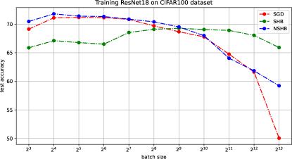
Figure 14: Test accuracy for SGD, SHB, and NSHB versus batch size in training ResNet18 on CIFAR100 dataset. This is the same graph shown in Figure 4.

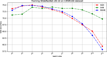
Figure 15: Test accuracy for SGD, SHB, and NSHB versus batch size in training WideResNet-28-10 on CIFAR100 dataset.

We measured test accuracy with batch sizes of $2^{3}$ to $2^{13}$ for 200 epochs for training ResNet18 (Figure 15) and with batch sizes of $2^{2}$ to $2^{11}$ for 200 epochs for training WideResNet-28-10 (Figure 15) with SGD, SHB, and NSHB on the CIFAR100 dataset. In both cases, the generalizability of SGD worsened as the batch size was increased, whereas that of SHB remained stable. Moreover, SHB achieved almost equal test accuracy from batch sizes of $2^{8}$ to $2^{12}$ for ResNet18 and from batch sizes of $2^{4}$ to $2^{9}$ for WideResNet-28-10. For very large batch sizes, i.e., $2^{13}$ for ResNet18 and $2^{10}$ and $2^{11}$ for WideResNet-28-10, accuracy decreased even though the degree of smoothing was the same. Note that these results are for 200 epochs for all batch sizes, meaning that the number of steps may have been insufficient for the larger batch sizes. When using the CIFAR100 dataset and 200 training epochs, the number of parameter update steps is $1,250,000$ for a batch size of $2^{3}$ but only $1400$ for a batch size of $2^{13}$.

F.2 Experiments on implicit graduated optimization with SHB

This section supplements the hyperparameter update rules in Figure 5 and provides the results for WideResNet-28-10 with Algorithm 3 (Figure 17). Recall that $\eta_{m+1}:=\kappa_{m}\eta_{m},b_{m+1}:=\lambda_{m}b_{m},\hat{\beta}_{m+1}:=\rho_{m}\hat{\beta}_{m}$, and

$$\frac{\kappa_{m}\eta_{m}\sqrt{(1+\rho_{m}\hat{\beta}_{m})\frac{C_{\text{\rm{SHB}}}^{2}}{\lambda_{m}b_{m}}+\rho_{m}\hat{\beta}_{m}K_{\text{\rm{SHB}}}^{2}}}{\eta_{m}\sqrt{(1+\hat{\beta}_{m})\frac{C_{\text{\rm{SHB}}}^{2}}{b_{m}}+\hat{\beta}_{m}K_{\text{\rm{SHB}}}^{2}}}=\gamma_{m}:=\frac{(M-m)^{0.9}}{\left\{M-(m-1)\right\}^{0.9}},$$

where $M=200,m\in[M],\kappa_{m},\rho_{m}\in(0,1],\lambda_{m}\geq 1$, and $\delta_{m+1}^{\text{\rm{SHB}}}:=\gamma_{m}\delta_{m}^{\text{\rm{SHB}}}$ is the degree of smoothing at epoch $m+1$.

The ”only lr decayed” method reduces only the learning rate, so the decay rate of noise level $\delta_{m+1}^{\text{\rm{SHB}}}/\delta_{m}^{\text{\rm{SHB}}}$ is equal to $\gamma_{m}$. Hence, we should use $\kappa_{m}:=\gamma_{m},\lambda_{m}:=1$, and $\rho_{m}:=1$ ; i.e., the ”only lr decayed” method means a polynomial decay rate of $p=0.9$. The ”only momentum decayed” method reduces only the momentum, so the decay rate of noise level $\delta_{m+1}^{\text{\rm{SHB}}}/\delta_{m}^{\text{\rm{SHB}}}$ is also equal to $\gamma_{m}$. Hence, we should use $\kappa_{m}:=1,\lambda_{m}:=1$, and $\rho_{m}$ such that

$$\frac{\sqrt{(1+\rho_{m}\hat{\beta}_{m})\frac{C_{\text{\rm{SHB}}}^{2}}{b}+\rho_{m}\hat{\beta}_{m}K_{\text{\rm{SHB}}^{2}}}}{\sqrt{(1+\hat{\beta}_{m})\frac{C_{\text{\rm{SHB}}}^{2}}{b}+\hat{\beta}_{m}K_{\text{\rm{SHB}}}^{2}}}=\gamma_{m}\ \text{ i.e., }\ \rho_{m}:=\frac{\gamma_{m}^{2}\left\{\frac{C_{\text{\rm{SHB}}}^{2}}{b}+\hat{\beta}_{m}\left(\frac{C_{\text{\rm{SHB}}}^{2}}{b}+K_{\text{\rm{SHB}}}^{2}\right)\right\}-\frac{C_{\text{\rm{SHB}}}^{2}}{b}}{\hat{\beta}_{m}\left(\frac{C_{\text{\rm{SHB}}}^{2}}{b}+K_{\text{\rm{SHB}}}^{2}\right)}.$$

Note that, since $\hat{\beta}_{m+1}:=\frac{\beta_{m+1}(\beta_{m+1}^{2}-\beta_{m+1}+1)}{(1-\beta_{m+1})^{2}}$, to find momentum $\beta_{m+1}$, we need to solve the cubic equation for $\beta_{m+1}$. The ”lr decayed and batch size increased” method reduces the learning rate and increases the batch size, so the decay rate of the noise level $\delta_{m+1}^{\text{\rm{SHB}}}/\delta_{m}^{\text{\rm{SHB}}}$ is also equal to $\gamma_{m}$. Hence, we should use $\rho_{m}:=1$, $\lambda_{m}:=\frac{(M-m)^{0.747}}{\left\{M-(m-1)\right\}^{0.747}}$, and $\kappa_{m}$ such that

$$\kappa_{m}:=\frac{\gamma_{m}\sqrt{(1+\rho_{m}\hat{\beta}_{m})\frac{C_{\text{\rm{SHB}}}^{2}}{\lambda_{m}b_{m}}+\rho_{m}\hat{\beta}_{m}K_{\text{\rm{SHB}}^{2}}}}{\sqrt{(1+\hat{\beta}_{m})\frac{C_{\text{\rm{SHB}}}^{2}}{b_{m}}+\hat{\beta}_{m}K_{\text{\rm{SHB}}}^{2}}},$$

where $\lambda_{m}$ was tuned so that when the initial batch size was $256$, increasing the batch size was still computationally small enough to run on our machines when 200 epochs were reached. For the remaining methods, the parameters were similarly updated so that the decay rate of the degree of smoothing was $\gamma_{m}:=\frac{(M-m)^{0.9}}{\left\{M-(m-1)\right\}^{0.9}}$.

Figure 16: Accuracy score for testing and loss function value for training versus epochs in training of ResNet18 on CIFAR100 dataset with implicit graduated optimization with SHB (Algorithm 3). This is the same graph shown in Figure 5.

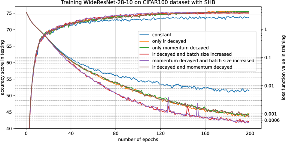
Figure 17: Accuracy score for testing and loss function value for training versus epochs in training of WideResNet-28-10 on CIFAR100 dataset with implicit graduated optimization with SHB (Algorithm 3).

F.3 Experiments on implicit graduated optimization with NSHB

To test the ability of Algorithm 5 to reduce stochastic noise, we compared a ”constant” method in which the learning rate, batch size, and momentum were all constant with a method in which the hyperparameters were updated to reduce the degree of smoothing $\delta^{\text{\rm{NSHB}}}$. Figures 19 and 19 plot the accuracy in testing and the loss function value in training with NSHB versus the number of epochs. We tuned the noise reduction methods so that the decay rate was $\gamma_{m}:=\frac{(M-m)^{0.9}}{\left\{M-(m-1)\right\}^{0.9}}\ (M=200,m\in[M])$.

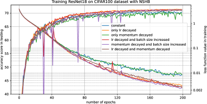
Figure 18: Accuracy score for testing and loss function value for training versus epochs in training of ResNet18 on CIFAR100 dataset with implicit graduated optimization with NSHB (Algorithm 5).

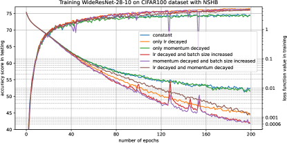
Figure 19: Accuracy score for testing and loss function value for training versus epochs in training of WideResNet-28-10 on CIFAR100 dataset with implicit graduated optimization with NSHB (Algorithm 5).

F.4 Experiments on optimal noise scheduling with SHB and NSHB

Sato and Iiduka identified the conditions that the decay rate $(\gamma_{m})_{m\in[M]}$ of noise $(\delta_{m})_{m\in[M]}$ must satisfy by considering the conditions necessary for the success of a graduated optimization algorithm for the new $\sigma$-nice function [53]. They found that decay rate $\gamma_{m}$ should satisfy

$$\frac{\sqrt{(m-M-\sqrt{2})^{2}-1}-1}{-(m-M-\sqrt{2})}\leq\gamma_{m}<1\ \left(m\in[M],p\in(0,1]\right).$$ (18)

From (2)-(4) in Section 4.1, the noise level, i.e., the degree of smoothing, is proportional to the learning rate, which immediately leads to the optimal decay rate of the decaying learning rate. Figure 21 plots the decay rate of the existing learning rate scheduler and the regions satisfying inequality (18) when $M=200$. Figure 21 is an enlarged version of Figure 21.

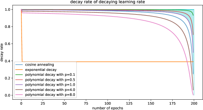
Figure 20: Decay rate of existing learning rate schedules. Blue-filled area represents regions satisfying inequality (18) when $M=200$.

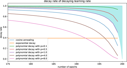
Figure 21: An enlarged version of Figure 21.

As shown in Figures 21 and 21, inequality (18) is satisfied by polynomial decay with $p\in(0,1]$ and not by any other learning rate scheduler. The rate of polynomial decay can be written as $\frac{(M-m)^{p}}{\left\{M-(m-1)\right\}^{p}}$, which is used in Algorithms 3 and 5. Figures 21 and 21 also show that polynomial decay with $p\in(0,1]$ may give the smallest loss function value through implicit graduated optimization. Sato and Iiduka confirmed this experimentally for SGD; i.e., they showed that polynomial decay with $p\in(0,1]$ can achieve the smallest training loss function value for SGD, as per theory [53]. We thus clarified whether polynomial decay with $p\in(0,1]$ can achieve the smallest loss function value for SGD with momentum as well.

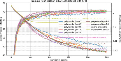
Figure 22: Accuracy score for testing and loss function value for training versus epochs in training of ResNet18 on CIFAR100 dataset with SHB and learning rate scheduler.

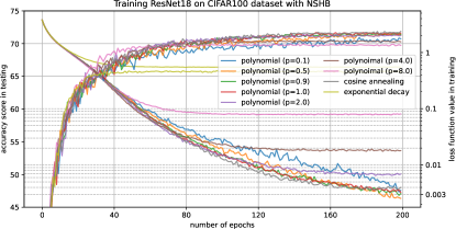
Figure 23: Accuracy score for testing and loss function value for training versus epochs in training of ResNet18 on CIFAR100 dataset with NSHB and learning rate scheduler.

Figures 23 and 23 plot test accuracy and training loss function values versus batch size for SHB and NSHB with learning rate scheduler in training of ResNet18 on the CIFAR100 dataset. The initial value of the learning rate was $0.1$, and the power of the exponential decay was $0.9$. The batch size and momentum were constants, $256$ and $0.9$, respectively.

Figures 25 and 25 plot test accuracy versus training loss function values for SHB and NSHB with learning rate scheduler in training of WideResNet-28-10 on the CIFAR100 dataset.

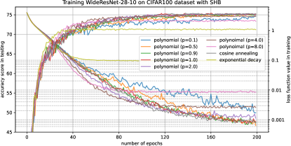
Figure 24: Accuracy score for testing and loss function value for training versus epochs in training of WideResNet-28-10 on CIFAR100 dataset with SHB and learning rate scheduler.

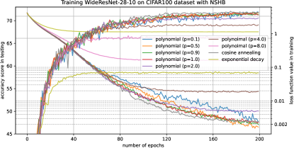
Figure 25: Accuracy score for testing and loss function value for training versus epochs in training of WideResNet-28-10 on CIFAR100 dataset with NSHB and learning rate scheduler.

Figures 23-25 show that polynomial decay with $p\in(0,1]$ can achieve the smallest loss function values among the learning rate schedulers. Note that when $p=0.1$, the loss function value fell more slowly than when $p\in\{0.5,0.9,1\}$. This can be explained by the convergence rate of Algorithms 3 and 5 being $\mathcal{O}\left(1/\epsilon^{\frac{1}{p}}\right)\ \left(p\in(0,1]\right)$. That is, the closer $p$ is to $1$, the fewer iterations are needed, so when $p=0.1$, we need many more iterations than when $p\in\{0.5,0.9,1\}$.

References

- An et al. [2018] Wangpeng An, Haoqian Wang, Qingyun Sun, Jun Xu, Qionghai Dai, and Lei Zhang. A PID controller approach for stochastic optimization of deep networks. In IEEE/CVF Conference on Computer Vision and Pattern Recognition, pages 8522–8531, 2018.
- Blake and Zisserman [1987] Andrew Blake and Andrew Zisserman. Visual Reconstruction. MIT Press, 1987.
- Bottou et al. [2018] Léon Bottou, Frank E. Curtis, and Jorge Nocedal. Optimization methods for large-scale machine learning. SIAM Review, 60(2):223–311, 2018.
- Chen et al. [2021] Jinghui Chen, Dongruo Zhou, Yiqi Tang, Ziyan Yang, Yuan Cao, and Quanquan Gu. Closing the generalization gap of adaptive gradient methods in training deep neural networks. In Proceedings of the Twenty-Ninth International Joint Conference on Artificial Intelligence, pages 3267–3275, 2021.
- Chen et al. [2022] John Chen, Cameron R. Wolfe, Zhao Li, and Anastasios Kyrillidis. Demon: Improved neural network training with momenutm decay. In IEEE International Conference on Acoustics, Speech and Signal Processing ICASSP, 2022.
- Chen et al. [2018] Liang-Chieh Chen, George Papandreou, Iasonas Kokkinos, Kevin Murphy, and Alan L. Yuille. Deeplab: Semantic image segmentation with deep convolutional nets, atrous convolution, and fully connected crfs. IEEE Transactions on Pattern Analysis and Machine Learning, 40(4):834–848, 2018.
- Chen et al. [2019] Xiangyi Chen, Sijia Liu, Ruoyu Sun, and Mingyi Hong. On the convergence of a class of Adam-type algorithms for non-convex optimization. Proceedings of the 7th International Conference on Learning Representations, 2019.
- Cutkosky and Mehta [2020] Ashok Cutkosky and Harsh Mehta. Momentum improves normalized SGD. In Proceedings of the 37th International Conference on Machine Learning, pages 2260–2268, 2020.
- Cyrus et al. [2018] Saman Cyrus, Bin Hu, Bryan Van Scoy, and Laurent Lessard. A robust accelerated optimization algorithm for strongly convex functions. In Annual American Control Conference, pages 1376–1381, 2018.
- Daneshmand et al. [2018] Hadi Daneshmand, Jonas Moritz Kohler, Aurélien Lucchi, and Thomas Hofmann. Escaping saddles with stochastic gradients. In Proceedings of the 35th International Conference on Machine Learning, pages 1163–1172, 2018.
- Defazio [2020] Aaron Defazio. Momentum via primal averaging: Theoretical insights and learning rate schedules for non-convex optimization. https://arxiv.org/abs/2010.00406, 2020.
- Duchi et al. [2010] John C. Duchi, Elad Hazan, and Yoram Singer. Adaptive subgradient methods for online learning and stochastic optimization. In Proceedings of the 23rd Conference on Learning Theory, pages 257–269, 2010.
- Fehrman et al. [2020] Benjamin Fehrman, Benjamin Gess, and Arnulf Jentzen. Convergence rates for the stochastic gradient descent method for non-convex objective functions. Journal of Machine Learning Research, 21:1–48, 2020.
- Fu et al. [2023] Jingwen Fu, Bohan Wang, Huishuai Zhang, Zhizheng Zhang, Wei Chen, and Nanning Zheng. When and why momentum accelerates SGD: An empirical study. https://arxiv.org/abs/2306.09000, 2023.
- Ge et al. [2015] Rong Ge, Furong Huang, Chi Jin, and Yang Yuan. Escaping from saddle points - online stochastic gradient for tensor decomposition. In Proceedings of the 28th Conference on Learning Theory, pages 797–842, 2015.
- Gitman et al. [2019] Igor Gitman, Hunter Lang, Pengchuan Zhang, and Lin Xiao. Understanding the role of momentum in stochastic gradient methods. In Advances in Neural Information Processing Systems, pages 9630–9640, 2019.
- Gupal and Bazhenov [1972] A.M. Gupal and L. T. Bazhenov. A stochastic analog of the conjugate gradient method. Cybernetics, 8(1):138–140, 1972.
- HaoChen et al. [2021] Jeff Z. HaoChen, Colin Wei, Jason D. Lee, and Tengyu Ma. Shape matters: Understanding the implicit bias of the noise covariance. In Proceedings of the 34th Conference on Learning Theory, pages 2315–2357, 2021.
- Hardt et al. [2016] Moritz Hardt, Ben Recht, and Yoram Singer. Train faster, generalize better: Stability of stochastic gradient descent. In Proceedings of The 33rd International Conference on Machine Learning, pages 1225–1234, 2016.
- Harshvardhan and Stich [2021] Harshvardhan and Sebastian U. Stich. Escaping local minima with stochastic noise. In the 13th International OPT Workshop on Optimization for Machine Learning in NeurIPS 2021, 2021.
- Hazan et al. [2016] Elad Hazan, Kfir Yehuda, and Shai Shalev-Shwartz. On graduated optimization for stochastic non-convex problems. In Proceedings of The 33rd International Conference on Machine Learning, pages 1833–1841, 2016.
- He et al. [2019] Fengxiang He, Tongliang Liu, and Dacheng Tao. Control batch size and learning rate to generalize well: Theoretical and empirical evidence. In Proceedings of the 32nd International Conference on Neural Information Processing Systems, pages 1141–1150, 2019.
- He et al. [2016] Kaiming He, Xiangyu Zhang, Shaoqing Ren, and Jian Sun. Deep residual learning for image recognition. In IEEE Conference on Computer Vision and Pattern Recognition, pages 770–778, 2016.
- Hundt et al. [2019] Andrew Hundt, Varun Jain, and Gregory D. Hager. sharpDARTS: faster and more accurate differentiable architecture search. https://arxiv.org/abs/1903.09900, 2019.
- Iiduka [2022a] Hideaki Iiduka. Appropriate learning rates of adaptive learning rate optimization algorithms for training deep neural networks. IEEE Transactions on Cybernetics, 52(12):13250–13261, 2022a.
- Iiduka [2022b] Hideaki Iiduka. Critical bach size minimizes stochastic first-order oracle complexity of deep learning optimizer using hyperparameters close to one. https://arxiv.org/abs/2208.09814, 2022b.
- Jelassi and Li [2022] Samy Jelassi and Yuanzhi Li. Towards understanding how momentum improves generalization in deep learning. In Proceedings of the 39th International Conference on Machine Learning, pages 9965–10040, 2022.
- Jin et al. [2017] Chi Jin, Rong Ge, Praneeth Netrapalli, Sham M. Kakade, and Michael I. Jordam. How to escape saddle points efficiently. http://arxiv.org/abs/1703.00887, 2017.
- Keskar et al. [2017] Nitish Shirish Keskar, Dheevatsa Mudigere, Jorge Nocedal, Mikhail Smelyanskiy, and Ping Tak Peter Tang. On large-batch training for deep learning: Generalization gap and sharp minima. In Proceedings of the 5th International Conference on Learning Representations, 2017.
- Kidambi et al. [2018] Rahul Kidambi, Praneeth Netrapalli, Prateek Jain, and Sham M. Kakade. On the insufficiency of existing momentum schemes for stochastic optimization. In Proceedings of the 6th International Conference on Learning Representations, 2018.
- Kingma and Ba [2015] Diederik P Kingma and Jimmy Lei Ba. Adam: A method for stochastic optimization. In Proceedings of the 3rd International Conference on Learning Representations, pages 1–15, 2015.
- Kleinberg et al. [2018] Robert Kleinberg, Yuanzhi Li, and Yang Yuan. An alternative view: When does SGD escape local minima? In Proceedings of the 35th International Conference on Machine Learning, pages 2703–2712, 2018.
- Krizhevsky [2009] Alex Krizhevsky. Learning multiple layers of features from tiny images. https://www.cs.toronto.edu/~kriz/learning-features-2009-TR.pdf, 2009.
- Kunstner et al. [2023] Frederik Kunstner, Jacques Chen, Jonathan Wilder Lavington, and Mark Schmidt. Noise is not the main factor behind the gap between SGD and adam on transformers, but sign descent might be. In Proceedings of the 8th International Conference on Learning Representations, 2023.
- Leclerc and Madry [2020] Guillaume Leclerc and Aleksander Madry. The two regimes of deep network training. https://arxiv.org/abs/2002.10376, 2020.
- Lessard et al. [2016] Laurent Lessard, Benjamin Recht, and Andrew K. Packard. Analysis and design of optimization algorithms via integral quadratic constraints. SIAM Journal on Optimization, 26(1):57–95, 2016.
- Li et al. [2019] Yuanzhi Li, Colin Wei, and Tengyu Ma. Towards explaining the regularization effect of initial large learning rate in training neural networks. In Advances in Neural Information Processing Systems, pages 11669–11680, 2019.
- Lin et al. [2016] Junhong Lin, Raffaello Camoriano, and Lorenzo Rosasco. Generalization properties and implicit regularization for multiple passes SGM. In Proceedings of The 33rd International Conference on Machine Learning, pages 2340–2348, 2016.
- Liu et al. [2020] Yanli Liu, Yuan Gao, and Wotao Yin. An improved analysis of stochastic gradient descent with momentum. In Advances in Neural Information Processing Systems, 2020.
- Loizou et al. [2021] Nicolas Loizou, Sharan Vaswani, Issam Laradji, and Simon Lacoste-Julien. Stochastic polyak step-size for SGD: An adaptive learning rate for fast convergence: An adaptive learning rate for fast convergence. In Proceedings of the 24th International Conference on Artificial Intelligence and Statistics (AISTATS), 2021.
- Loshchilov and Hutter [2017] Ilya Loshchilov and Frank Hutter. SGDR: stochastic gradient descent with warm restarts. In Proceedings of the 5th International Conference on Learning Representations, 2017.
- Ma and Yarats [2019] Jerry Ma and Denis Yarats. Quasi-hyperbolic momentum and adam for deep learning. In Proceedings of the 7th International Conference on Learning Representations, 2019.
- Ma et al. [2018] Siyuan Ma, Raef Bassily, and Mikhail Belkin. The power of interpolation: Understanding the effectiveness of SGD in modern over-parametrized learning. Proceedings of the 35th International Conference on Machine Learning, 80:3331–3340, 2018.
- McCandlish et al. [2018] Sam McCandlish, Jared Kaplan, Dario Amodei, and OpenAI Dota Team. An empirical model of large-batch training. http://arxiv.org/abs/1812.06162, 2018.
- Mou et al. [2018] Wenlong Mou, Liwei Wang, Xiyu Zhai, and Kai Zheng. Generalization bounds of SGLD for non-convex learning: Two theoretical viewpoints. In Proceedings of the 31st Annual Conference on Learning Theory, pages 605–638, 2018.
- Nesterov [1983] Y. Nesterov. A method for unconstrained convex minimization problem with the rate of convergence . Doklady AN USSR, 269:543–547, 1983.
- Paszke et al. [2019] Adam Paszke, Sam Gross, Francisco Massa, Adam Lerer, James Bradbury, Gregory Chanan, Trevor Killeen, Zeming Lin, Natalia Gimelshein, Luca Antiga, Alban Desmaison, Andreas Köpf, Edward Z. Yang, Zachary DeVito, Martin Raison, Alykhan Tejani, Sasank Chilamkurthy, Benoit Steiner, Lu Fang, Junjie Bai, and Soumith Chintala. PyTorch: An imperative style, high-performance deep learning library. In Advances in Neural Information Processing Systems, pages 8024–8035, 2019.
- Polyak [1964] B.T. Polyak. Some methods of speeding up the convergence of iteration methods. USSR Computational Mathematics and Mathematical Physics, 4(5):1–17, 1964.
- Reddi et al. [2018] Sashank J. Reddi, Satyen Kale, and Sanjiv Kumar. On the convergence of adam and beyond. In Proceedings of the 6th International Conference on Learning Representations, 2018.
- Robbins and Monro [1951] Herbert Robbins and Sutton Monro. A stochastic approximation method. The Annals of Mathematical Statistics, 22:400–407, 1951.
- Rose et al. [1990] Kenneth Rose, Eitan Gurewitz, and Geoffrey Fox. A deterministic annealing approach to clustering. Pattern Recognition Letters, 11(9):589–594, 1990.
- Sato and Iiduka [2023a] Naoki Sato and Hideaki Iiduka. Existence and estimation of critical batch size for training generative adversarial networks with two time-scale update rule. In Proceedings of the 40th International Conference on Machine Learning, pages 30080–30104, 2023a.
- Sato and Iiduka [2023b] Naoki Sato and Hideaki Iiduka. Using stochastic gradient descent to smooth nonconvex functions: Analysis of implicit graduated optimization with optimal noise scheduling. https://arxiv.org/abs/2311.08745, 2023b.
- Scaman and Malherbe [2020] Kevin Scaman and Cedric Malherbe. Robustness analysis of non-convex stochastic gradient descent using biased expectations. In Proceedings of the 34th Conference on Neural Information Processing Systems, pages 16377–16387, 2020.
- Scoy et al. [2018] Bryan Van Scoy, Randy A. Freeman, and Kevin M. Lynch. The fastest known globally convergent first-order method for minimizing strongly convex functions. IEEE Control Systems Letters, 2(1):49–54, 2018.
- Shallue et al. [2019] Christopher J. Shallue, Jaehoon Lee, Joseph M. Antognini, Jascha Sohl-Dickstein, Roy Frostig, and George E. Dahl. Measuring the effects of data parallelism on neural network training. Journal of Machine Learning Research, 20(112):1–49, 2019.
- Smith et al. [2018] Samuel L. Smith, Pieter-Jan Kindermans, Chris Ying, and Quoc V. Le. Don’t decay the learning rate, increase the batch size. In Proceedings of the 6th International Conference on Learning Representations, 2018.
- Sutskever et al. [2013] Ilya Sutskever, James Martens, George E. Dahl, and Geoffrey E. Hinton. On the importance of initialization and momentum in deep learning. In Proceedings of the 30th International Conference on Machine Learning, pages 1139–1147, 2013.
- Wen et al. [2020] Yeming Wen, Kevin Luk, Maxime Gazeau, Guodong Zhang, Harris Chan, and Jimmy Ba. An empirical study of large-batch stochastic gradient descent with structured covariance noise. In Proceedings of the 23rd International Conference on Artificial Intelligence and Statistics AISTATS, pages 3621–3631, 2020.
- Wu et al. [2014] Yuting Wu, Daniel J. Holland, Mick D. Mantle, Andrew Gordon Wilson, Sebastian Nowozin, Andrew Blake, and Lynn F. Gladden. A bayesian method to quantifying chemical composition using NMR: application to porous media systems. In Proceedings of the 22nd European Signal Processing Conference (EUSIPCO), pages 2515–2519, 2014.
- Wu [1996] Zhijun Wu. The effective energy transformation scheme as a special continuation approach to global optimization with application to molecular conformation. SIAM Journal on Optimization, 6(3):748–768, 1996.
- Zagoruyko and Komodakis [2016] Sergey Zagoruyko and Nikos Komodakis. Wide residual networks. In Proceedings of the British Machine Vision Conference, 2016.
- Zaheer et al. [2018] Manzil Zaheer, Sashank J. Reddi, Devendra Sachan, Satyen Kale, and Sanjiv Kumar. Adaptive methods for nonconvex optimization. In Proceedings of the 32nd International Conference on Neural Information Processing Systems, 2018.
- Zhang et al. [2019] Guodong Zhang, Lala Li, Zachary Nado, James Martens, Sushant Sachdeva, George E. Dahl, Christopher J. Shallue, and Roger B. Grosse. Which algorithmic choices matter at which batch sizes? insights from a noisy quadratic model. In Advances in Neural Information Processing Systems, pages 8194–8205, 2019.
- Zhou et al. [2020] Dongruo Zhou, Jinghui Chen, Yuan Cao, Yiqi Tang, Ziyan Yang, and Quanquan Gu. On the convergence of adaptive gradient methods for nonconvex optimization. 12th Annual Workshop on Optimization for Machine Learning, 2020.
- Zhuang et al. [2020] Juntang Zhuang, Tommy Tang, Yifan Ding, Sekhar Tatikonda, Nicha C. Dvornek, Xenophon Papademetris, and James S. Duncan. AdaBelief optimizer: Adapting stepsizes by the belief in observed gradients. In Advances in Neural Information Processing Systems, 2020.
- Zou et al. [2019] Fangyu Zou, Li Shen, Zequn Jie, Weizhong Zhang, and Wei Liu. A sufficient condition for convergences of adam and rmsprop. 2019 IEEE/CVF Conference on Computer Vision and Pattern Recognition (CVPR), pages 11119–11127, 2019.