INViT: A Generalizable Routing Problem Solver
with Invariant Nested View Transformer

Abstract

Recently, deep reinforcement learning has shown promising results for learning fast heuristics to solve routing problems. Meanwhile, most of the solvers suffer from generalizing to an unseen distribution or distributions with different scales. To address this issue, we propose a novel architecture, called Invariant Nested View Transformer (INViT), which is designed to enforce a nested design together with invariant views inside the encoders to promote the generalizability of the learned solver. It applies a modified policy gradient algorithm enhanced with data augmentations. We demonstrate that the proposed INViT achieves a dominant generalization performance on both TSP and CVRP problems with various distributions and different problem scales. Both code and data are available in supplementary materials.

I Introduction

Among all combinatorial optimization problems, routing problems, such as traveling salesman problem (TSP) or vehicle routing problem (VRP), are arguably among the most studied thanks notably to their wide application range, such as logistics [1], electronic design automation [2], or bioinformatics [3]. Due to their NP-hard nature, exact algorithms are impracticable for solving large-scale instances, which has motivated the active development of approximate heuristic methods. Although state-of-the-art (SOTA) heuristic methods, such as LKH3 [4, 5] or HGS [6], have been designed to provide high-quality solutions for large routing problem instances with higher efficiency, the computational costs remain prohibitively high.

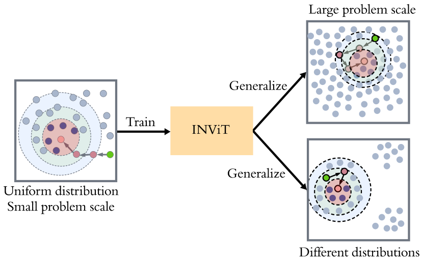
Figure 1: Our method INViT aggregates node information from multiple nested local views (marked as colored discs). Trained on small instances following uniform distributions, INViT can generalize to instances with larger sizes or/and different distributions.

To obtain faster heuristics, researchers have started to actively explore the exploitation of deep learning, and especially deep reinforcement learning (DRL), either (1) to learn to construct [7, 8], in which case the learned solver generates a solution step by step, or (2) to learn to search [9, 10, 11, 12], in which case the learned solver guides a local search method. In this paper, we focus on neural constructive methods, which usually enjoy faster inference while still reaching good performance compared with learn-to-search methods.

While constructive solvers demonstrate promising results, the existing DRL-based models generally lack robust generalization abilities, as also previously noted by Joshi et al. [13]. Indeed, those models are usually trained on fixed-scale (e.g., small) instances drawn from a fixed (e.g., uniform) probability distribution, but, once trained, they are incapable of generating satisfactory solutions on new instances of larger scales (i.e., cross-size generalization) or drawn from a different distribution (i.e., cross-distribution generalization). While one may think of training on more diverse instances (larger scales or drawn from more diverse distributions) to address this generalization issue, this comes with an increased computational cost, which may be completely impractical for huge instances. Moreover, after deployment, new instances with larger scales or drawn from unseen distributions may always happen.

In this paper, our objective is to develop a constructive (a.k.a. autoregressive) solver with strong generalization capabilities, ensuring stable performance irrespective of distribution or scale, while also maintaining low time and memory complexity. To that aim, we analyze previous models and identify two main sources for the generalization issue: embedding aliasing and interference from irrelevant nodes. The first source describes the situation where trained neural models fail to distinguish nodes in higher-density regions of a routing problem instance, as this can happen when increasing instance sizes or when drawing from a non-uniform distribution. The second source happens in particular in Transformer-based models where the self-attention weights take into account all the nodes, even the farthest ones, which are usually not relevant when constructing a solution. As a countermeasure against these two phenomena, we propose the removal of nodes far from the last visited one in both the action and state spaces, which we justify by careful statistical analyses of optimal solutions in routing problems.

Motivated by our previous observations, we propose Invariant Nested View Transformer (INViT), which combines graph sparsification and invariance, to address the generalization issue (see Figure 1). More specifically, INViT is a Transformer-based architecture that processes multiple nested local views centered around the last visited node, where the smallest view only includes the most promising candidate actions, while the other larger views provide the most relevant state information for action selection.

Our contributions can be summarized as follows:

• We identify two factors explaining the generalization issue observed in most previous DRL-based methods: embedding aliasing and interference from irrelevant nodes. By analyzing some statistical properties of optimal solutions of routing problems, we motivate the reduction of the state and action spaces.

• We design a novel Transformer-based architecture that takes invariant nested views of a routing problem instance. Its architecture is justified by our previous observations and statistical analyses.

• We demonstrate on different datasets that the proposed architecture outperforms the current SOTA methods in terms of the generalization on both TSP and CVRP.

II Related Work

Recently, research investigating the application of deep learning and DRL to solve combinatorial optimization problems has become very active, exploring both local search and constructive methods. For space reasons, we focus our discussion on the most related work for neural constructive methods. In this literature, both novel architectures and novel DRL training algorithms have been proposed. Our work mainly contributes in the first direction.

Architectures.

Initial work in this direction proposed and studied various architectures, such as Pointer Network [14], Attention Model [7], and Graph Neural Network (GNN) [15]. Apart from the latter one based on supervised learning, most studies consider reinforcement learning (RL), usually resorting to the simple REINFORCE algorithm [16]. To the best of our knowledge, S2V-DQN [17], a sequence-to-vector architecture, trained by DQN [18], is the first method to explicitly consider cross-size generalization.

The Attention Model [7] is based on the Transformer architecture [19]. Given its generic nature and its promising performance, recent work has focused on improving its architecture. For instance, PointerFormer [8] develops a multi-pointer network to achieve better performance. MVGCL [20] combines a GNN encoder followed by an attention-based encoder, where the former is trained by contrastive learning to leverage graph information for cross-distribution generalization. ELG proposed very recently [21], is an ensemble model comprised of a global policy and local policies, whose outputs are aggregated with a pre-fixed rule. The local policies, utilizing k-nearest neighbors (k-NN) promote cross-size generalizability.

While ELG and our architecture share some superficial similarities (e.g., use of k-NN to create local views), there are some key differences, which make our proposition superior in terms of generalization performance. For instance, our method learns to aggregate the local views in the embedding space. This directly tackles embedding aliasing, which is further reduced by considering nested local views in our method. In addition, our architecture does not include a global view, since the use of a global encoder may be detrimental to the overall performance, as suggested by our statistical analysis (see Section III.2).

Training Algorithms.

Most work applies standard RL algorithms, but some recent propositions specifically aim at improving the training (and also inference) algorithm. For instance, POMO [22] includes a generic technique, which can significantly enhance the performance of neural solvers with minimal additional costs: it generates multiple solutions by considering shifted starting nodes or by applying invariant transformations to input instances. Like other recent works [8, 21], we also apply this simple but effective idea.

Regarding the generalization issue, some works aim at improving cross-size generalization, e.g., using meta RL [23] or exploiting equivariance and local search [24, 25]. Others focus on cross-distribution generalization, e.g., using a specifically-designed new loss [26] or via knowledge distillation [27]. Recently, Omni-TSP/VRP [28], inspired by the meta-RL approach proposed by Qiu et al. [23], tackles both cross-size and cross-distribution generalization, as we do in our work. The latter work is therefore a good SOTA baseline to compare with our proposition.

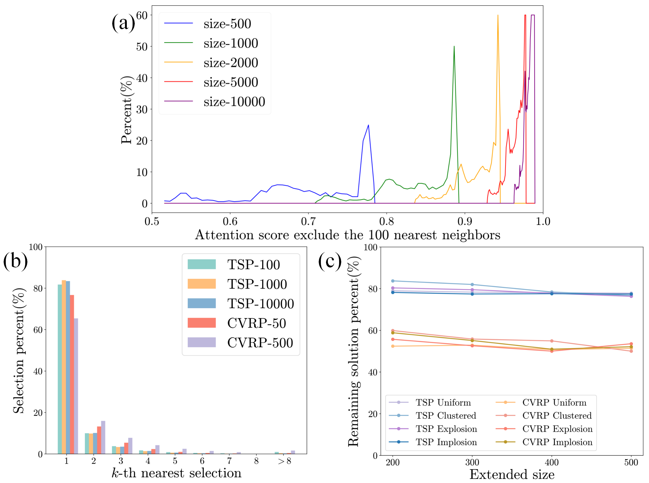
Figure 2: Preliminary findings. (a) The histogram of attention score for farther nodes in attention-based encoders (trained on TSP/CVRP 100). (b) The histogram of the optimal solution in $k$-th nearest neighbors for different $k$. (c) The percentage overlap of optimal solutions between the original and augmented instances.

III Background and Motivation

Before introducing the motivation of INViT, we first recall the basic formulation of routing problems and the common mechanism of autoregressive solvers. Then based on our preliminary experiments, we point out the potential problems on generalization of the autoregressive solvers and propose some initial ideas to address those problems.

III.1 Autoregressive Solvers for Routing Problems

Euclidean Routing Problem.

Assume we are given a Euclidean Routing Problem instance $x$ with a graph $\mathcal{G}$ and a set of constraints. The graph $\mathcal{G}$ is composed of a node set $\mathcal{C}=\{c_{1},c_{2},\ldots,c_{n}\}$ and an edge set $\mathcal{E}$ contains all connections between nodes. A feasible solution $F_{x}$ is an index sequence $(f_{1},\cdots,f_{\ell})$ of length ${\ell}$ that satisfies all the constraints. Basically, each node $c_{i}$ has a coordinate $(c_{i}^{1},c_{i}^{2})\in[0,1]^{2}$. The cost is defined by $D_{x}({F}_{x})=d(c_{f_{\ell}},c_{f_{1}})+\sum_{t=1}^{{\ell}-1}d(c_{f_{t}},c_{f_{t+1}})\,,$ where $d$ is the Euclidean distance. Our goal is to find a feasible solution that minimizes the cost function. The constraints vary according to the specific Routing Problem. For TSP, the only constraint is that the agent has to visit all the nodes exactly once. For VRP, an extra set of variable, demands, is introduced to constrain the behavior of the agent. Each node $c_{i}$ has a demand $z_{i}$ to fulfill and the agent has a fixed capacity $R$. A depot node $c_{0}$ is introduced for the agent to replenish when it runs out of its capacity. In Capacitated VRP (CVRP), the agent is constrained to visit nodes except depot strictly once.

Autoregressive Solvers.

Such a solver starts from an initial node, and repeatedly selects the next node to visit, until it outputs a feasible solution. Regarding this process as a Markov decision process (MDP), at time step $t$, a state $s_{t}$ consists of a partial solution $(c_{f_{1}},\cdots,c_{f_{t}})$ and a remaining graph $\mathcal{G}_{t}=\left(\mathcal{C}_{t},\mathcal{E}_{t}\right)$. As noticed by Kool et al. [7], the stateful partial solution can be reduced to the first visited node/depot and the last visited node $(c_{f_{1}},c_{f_{t}})$. A solver calculates a probability $p_{\theta}(a_{t}|s_{t})$ for each action $a_{t}$ (i.e., node to be visited at time $t$) given the observable state $s_{t}$. By the chain rule, the joint probability of a feasible solution is given by:

$$p_{\theta}\left({F}_{x}|x\right)=\prod_{t=1}^{{\ell}}p_{\theta}(a_{t}|s_{t}).$$ (1)

The REINFORCE [16] algorithm can train an autoregressive solver using gradient $\nabla_{\theta}\mathcal{L}(\pi_{\theta})$ defined by:

$$\mathbb{E}_{p_{\theta}}\left[\left(D_{x}\left({F}_{x}\right)-b(x)\right)\nabla_{\theta}\log\prod_{t=1}^{{\ell}}p_{\theta}(a_{t}|s_{t})\right],$$ (2)

where $b(x)$ represents a baseline performance.

III.2 Generalization Issue in Embedding Space

To design an autoregressive solver that can generalize well both in the cross-size and cross-distribution settings, we first identify two shortcomings of current neural solvers trained on small scale and uniform distributed instances: embedding aliasing and interference from irrelevant nodes.

Embedding Aliasing.

Recall that (deep) neural networks are simply Lipschitz functions [29]. Let $h$ denotes the encoder layer of a neural solver trained on uniformly-distributed instances in the unit square, with size bounded by $n$. Then, $h$ would satisfy the following Lipschitz inequality:

$$\left\|h(c_{i})-h(c_{j})\right\|\leq L\left\|c_{i}-c_{j}\right\|,\qquad\forall c_{i},c_{j}\in\mathcal{C}$$ (3)

where $L>0$ is the Lipschitz constant.

After training, encoder $h$ should be able to usually distinguish nodes whose expected minimum pairwise distance in the unit square is $O(1/n)$. However, when considering a new uniformly-distributed instance whose size $N$ is larger than $n$, encoder $h$ would have to distinguish nodes whose expected minimum pairwise distance is $O(1/N)<O(1/n)$. Because of the Lipschitz inequality, there will be necessarily a size $N$ such that the embeddings produced by encoder $h$ will be mixed up, leading to incorrect action choices by the neural solver.

We call this phenomenon embedding aliasing, which provides one partial explanation to the generalization issues observed in existing neural solvers. Note that embedding aliasing can also occur when considering different distributions. Indeed, a non-uniform distribution will necessarily generate some regions that contain densely packed nodes.

Interference from Irrelevant Nodes.

The second issue mostly impacts attention-based solvers that process the complete graph directly. Recall that one attention layer computes the following embeddings:

$$\bm{E}=\texttt{Softmax}\left(\frac{QK^{\top}}{\sqrt{d_{K}}}\right)V.$$ (4)

where $Q,K,V$ correspond to query, key and value. For node $c_{j}$, its impact on the embedding of node $c_{i}$ is given by the attention score between $Q_{i}$ and $K_{j}$. After training, the encoder may learn to assign lower attention scores to irrelevant nodes (i.e., far away nodes in routing problems), however, the cumulative impact of those irrelevant nodes becomes non-negligible as the instance size increases, as illustrated in Figure 2 (a), which shows the empirical distribution of the sum of attention scores after excluding the 100 closest neighbors for a given model trained on instance size 100. Mechanically, the contribution of those irrelevant nodes may impact the new embeddings, further amplifying the embedding aliasing issue.

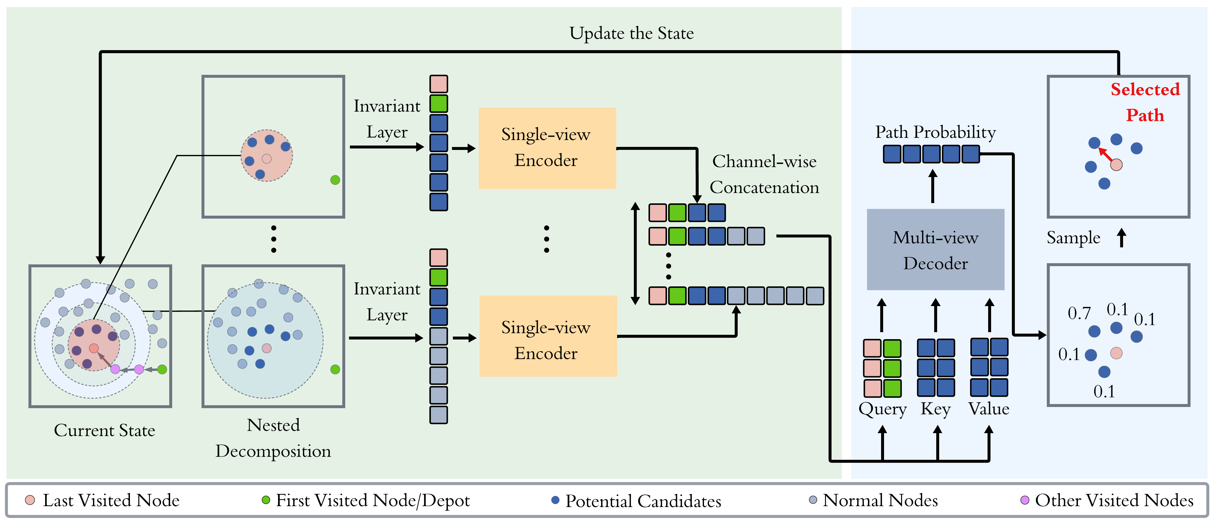
Figure 3: The overall architecture of INViT. The input state is extracted into multiple nested views, consisting of neighborhood nodes around the last visited node. Nodes located in the smallest view are potential candidates, and other nodes located in the view are called normal nodes. Each nested view is processed by a single-view encoder to obtain the embeddings for each node. Embeddings are then concatenated channel-wisely across different views. The decoder takes the embeddings of the last visited node and the first visited node (or depot) as the query, and the embeddings of the potential candidates as the key and the value. Lastly, the model samples a node to visit by the output probabilities. It updates the partial tour in an autoregressive manner until a complete tour is constructed.

III.3 Preliminary Findings

The previous observations suggest to control the number of nodes given as inputs of a neural solver. Interestingly, both the action and state spaces could be reduced.

Action Space.

While theoretically, the action space should contain all nodes that satisfy the constraints of a problem (e.g., unvisited node in TSP or unvisited node whose demand is less than the current capacity in CVRP). In practice, only the closest nodes need to be considered, as justified by Figure 2 (b), which shows the distribution of the rank in terms of neareast neighbors for any node in an optimal solution both in random TSP and CVRP with different scales. This observation, which is quite natural since an optimal solution minimizes a sum of distances, indicates that we can reduce our action space to a smaller subset, composed of the closest neighbors of the last visited node within the original action space (e.g., 8-NN can include $>$98% of optimal choices).

State Space.

While the action space can be narrowed down, the action choice can still depend on eliminated nodes. Indeed, they could provide useful information regarding the future impact. To simulate node elimination, we instead add randomly-distributed nodes outside the unit square for different random instances. Figure 2 (c) measures the percentage of edges that appear both in the optimal solutions of the initial random instances and in those of the augmented instances. These results indicate that the eliminated actions have a relatively limited impact on the optimal choices for TSP. In CVRP, the impact is larger, due to the capacity constraint, which can result in larger changes of the optimal solution. However, since the effects are not as pronounced as for the action space and because of the two issues described in Section III.2, a state space reduction with several nested sets may be beneficial.

IV Method

We present Invariant Nested View Transformer (INViT). We address the problems in Section III.2 by implementing the observations in Section III.3 into the model design.

IV.1 Invariant Nested View Transformer

The overall architecture and the autoaggressive workflow are shown in Figure 3. INViT incorporates a collection of nested-view encoders to embed the node features and maintains invariant views irrespective of the distribution and scale. According to Section III.2, we define a set of neighbors of the last visited node as potential candidate set $\mathbb{A}^{p}$, which corresponds to the smallest view in Figure 3. It’s noteworthy that in VRP, the depot is typically considered as a candidate, since the agent is only prohibited from revisiting the depot when it is currently located there.

Nested View Encoders.

As illustrated in Section III.2, the complete graph assumption allows farther nodes to have an exaggerated impact on the embeddings. To tackle this issue, one simple approach is to perform sparsification on the graph. Calculating a sparse graph for a static graph is a feasible task. However, taking into account the dynamic nature of the routing problem, computing a dynamically sparse graph during the inference procedure becomes a computationally expensive task. Hence, we present a nested view encoder design to tackle this issue by sparsifying the graph into subgraphs, each composed of different numbers of neighbors. As the k-nearest neighbor (k-NN) algorithm can offer stable neighbors and operate in a batch manner, we employ it to perform graph sparsification. By eliminating the nodes which are not in neighbors with different k, multiple subgraphs are produced. After proceeding with the invariant layer, each parallel single-view encoder would receive a distinct invariant subgraph and output the embeddings under different graph-contexts. The nested view design enables INViT to integrate the embedding with different correlations, emphasizing the correlations between highly related nodes while preserving some correlations between less related nodes.

Invariant Layer.

As shown in Section III.2, most of the encoders struggle to distinguish close nodes when the distance between nodes becomes sufficiently small. It is another key factor that hurts the generalization capability of attention-based encoders. Therefore, to overcome the problem, we designed a layer called Invariant Layer. The Invariant Layer consists of two steps: normalization and projection. The normalization could be formulated as follows:

$$\hat{c}^{m}_{i}=\frac{c^{m}_{i}-\min_{j\in\mathbb{N}}c^{m}_{j}}{\max_{m\in\left\{1,2\right\}}\max_{i,j\in\mathbb{N}}|c_{i}^{m}-c_{j}^{m}|}.$$ (5)

As shown in Figure 3, in addition to the potential candidate set $\mathbb{A}^{p}$ and the last visited node, the subgraph also includes the first visited node (or depot), the impact of which cannot be neglected. However, it is possible the first visited node (or depot) falls outside the region of the potential candidate set $\mathbb{A}^{p}$ and the last visited node, potentially compromising the effectiveness of the normalization process. In cases where the first visited node (or depot) cannot be visited, we incorporate a projection step, which could be formulated as

$$\hat{c}^{m}_{0}=\texttt{clip}\left(\frac{c^{m}_{0}-\min_{j\in\mathbb{N}}c^{m}_{j}}{\max_{m\in\left\{1,2\right\}}\max_{i,j\in\mathbb{N}}|c_{i}^{m}-c_{j}^{m}|},0,1\right),$$ (6)

where $\texttt{clip}(u,v,w)=\max(v,\min(u,w))$ projects the out-of-region first visited node (or depot) to the boundary, ensuring an invariant boundary for its coordinate.

Single-view Encoder.

Following the nested view design, multiple independent encoders are constructed to embed node features for different subgraphs. Once processed by the invariant layer, the subgraph is then input to the respective single-view encoder. The single-view encoder is composed of an initial linear layer and several encoder blocks consisting of Multi-Head Attention modules and Feed Forward layers [19]. To note that, the encoder does not use the positional encoding module, as the order of the input sequence is irrelevant to the Routing Problem. In alignment with the design of the invariant layer, which encompasses normalization and projection on different nodes, distinct initial linear layers are applied to capture node features. For each input subgraph, its node embeddings are produced by the corresponding single-view encoder.

Multi-view Decoder.

INViT aggregates multiple single-view embeddings by a channel-wise concatenation then inputs to a multi-view decoder after processing subgraphs by parallel single-view encoders. As mentioned previously, each subgraph shares a common intersection of nodes, which is the potential candidate set $\mathbb{A}^{p}$, the last visited nodes, and the first visited nodes (or depot). Discarding all the embeddings for those nodes outside this intersection, we can construct multi-view embeddings by channel-wisely concatenating single-view embeddings. The embeddings of the last visited node and the first visited node (or depot) are input as the query for the decoder, while the other embeddings of potential candidates serve as the key and the value in the decoder. The final output probability is the attention weight of the last layer, which could be formulated as

$$\pi_{t}(a)=\left\{\begin{array}[]{lr}\texttt{Softmax}\left(C\cdot\tanh\left(\frac{Q\cdot K^{T}}{\sqrt{d_{K}}}\right)\right),&a\in\mathbb{A}^{p}\\ 0,&\text{Otherwise}\\ \end{array}\right.$$ (7)

where $C$ is a positive constant. With the probability map, the next node could be sampled, and the entire model operates in an autoregressive manner.

IV.2 Algorithm

Training Stage.

To train INViT, we apply a REINFORCE-based algorithm integrated with data augmentation. Initially, two identical models are initialized with training parameter $\theta$ and baseline parameter $\theta^{\texttt{BL}}$. At the training stage, random instances are generated for training. For each training instance $x_{i}$, a set of augmented instances $\mathcal{X}_{i}=\{x_{i,j}\}_{j=1}^{\omega}$ is generated using the augmentation function, which includes rotation, reflection, and normalization. Leveraging the idea of Kwon et al. [22], we also introduce variation in the starting point for each augmented instance. According to Equation 2, the loss is computed based on the model performance and baseline performance. Following Kool et al. [7], the baseline tour is determined using the baseline model with a greedy rollout, while the model tour is computed using the training model with a random sampling strategy. The performance is then calculated as follows:

$$b(x_{i})=\mathbb{E}_{x\in\mathcal{X}_{i}}\left[D_{x}\left({F}_{x}(\mu_{\theta^{\texttt{BL}}})\right)\right],$$ (8)

$$D_{x_{i}}({F}_{x_{i}})=\mathbb{E}_{x\in\mathcal{X}_{i}}\left[D_{x}\left({F}_{x}(\pi_{\theta})\right)\right],$$

where ${F}_{x}(\pi)$ denotes the tour of instance $x$ under policy $\pi$, and $\mu$ is the deterministic policy induced by $\pi$.

Test Stage.

At the test stage, we also employ data augmentation to enhance overall performance. In contrast to the training stage, where we aim to use the average performance to increase generalizability on augmented instances, we only seek the best solution at the test stage. A comparison between the baseline model and training model is conducted at the end of each training epoch. If the training model outperforms the baseline model, its parameters $\theta^{\texttt{BL}}$ are substituted using the training parameter $\theta$.

V Experimental Results

To validate the generalizability of the proposed INViT, we use a series of datasets across various scales and distributions. We also include a comprehensive evaluation of our method, with several SOTA baselines, on our generated datasets and well-known public datasets.

Table 1: Performance on TSP problems with different distributions and problem scales.

Distribution	Uniform						Clustered
Category	TSP-100		TSP-1000		TSP-10000		TSP-100		TSP-1000		TSP-10000
Measurements	gap(%)	time	gap(%)	time	gap(%)	time	gap(%)	time	gap(%)	time	gap(%)	time
POMO(NeurIPS-20)	$1.29$	$2.0$m	$49.57$	$1.6$m	$84.99$	$3.8$m	$3.89$	$1.7$m	$50.36$	$1.6$m	$102.50$	$3.9$m
PointerFormer(AAAI-23)	$\bm{0.43}$	$1.7$m	$34.29$	$1.6$m	$71.85$	$3.9$m	$3.96$	$1.7$m	$43.89$	$1.6$m	$103.70$	$3.9$m
Omni-TSP(ICML-23)	$2.55$	$2.0$m	$20.25$	$1.9$m	$62.56$	$4.2$m	$3.62$	$2.0$m	$23.13$	$1.9$m	$71.47$	$4.2$m
ELG-v1	$0.51$	$3.2$m	$11.81$	$3.4$m	$20.83$	$10.1$m	$3.69$	$3.2$m	$17.67$	$3.0$m	$38.94$	$10.2$m
INViT-2V	$2.33$	$3.0$m	$6.40$	$3.5$m	$6.21$	$7.7$m	$3.39$	$2.9$m	$9.05$	$3.3$m	$\bm{9.29}$	$7.6$m
INViT-3V	$2.17$	$4.2$m	$\bm{6.31}$	$4.8$m	$\bm{6.08}$	$10.3$m	$\bm{2.99}$	$4.0$m	$\bm{8.95}$	$4.8$m	$\bm{9.29}$	$10.5$m
Distribution	Explosion						Implosion
Category	TSP-100		TSP-1000		TSP-10000		TSP-100		TSP-1000		TSP-10000
Measurements	gap(%)	time(s)	gap(%)	time(s)	gap(%)	time(s)	gap(%)	time(s)	gap(%)	time(s)	gap(%)	time(s)
POMO(NeurIPS-20)	$1.42$	$1.7$m	$50.00$	$1.6$m	$92.66$	$3.8$m	$1.44$	$1.7$m	$50.01$	$1.6$m	$88.02$	$3.8$m
PointerFormer(AAAI-23)	$\bm{0.87}$	$1.7$m	$40.99$	$1.6$m	$104.85$	$3.8$m	$\bm{0.71}$	$1.7$m	$35.21$	$1.6$m	$74.57$	$3.9$m
Omni-TSP(ICML-23)	$3.21$	$2.0$m	$21.97$	$1.9$m	$66.72$	$4.2$m	$2.67$	$2.0$m	$20.29$	$1.9$m	$63.85$	$4.2$m
ELG-v1	$0.93$	$3.5$m	$15.32$	$3.0$m	$35.03$	$9.8$m	$0.85$	$3.2$m	$12.10$	$3.1$m	$21.69$	$9.8$m
INViT-2V	$2.37$	$3.1$m	$8.74$	$3.5$m	$9.57$	$7.6$m	$2.61$	$2.9$m	$7.00$	$3.4$m	$6.96$	$7.6$m
INViT-3V	$2.15$	$4.3$m	$\bm{8.55}$	$4.7$m	$\bm{9.19}$	$10.2$m	$2.51$	$4.0$m	$\bm{6.95}$	$4.8$m	$\bm{6.87}$	$10.4$m

Table 2: Performance on CVRP problems with different distributions and problem scales.

Distribution	Uniform						Clustered
Category	CVRP-50		CVRP-500		CVRP-5000		CVRP-50		CVRP-500		CVRP-5000
Measurements	gap(%)	time(s)	gap(%)	time(s)	gap(%)	time(s)	gap(%)	time(s)	gap(%)	time(s)	gap(%)	time(s)
POMO(NeurIPS-20)	$6.01$	$1.5$m	$32.85$	$1.4$m	$277.63$	$1.8$m	$6.68$	$1.5$m	$26.80$	$1.4$m	$182.90$	$1.9$m
Omni-VRP(ICML-23)	$5.15$	$1.8$m	$\bm{7.06}$	$1.6$m	$36.17$	$2.0$m	$\bm{3.84}$	$1.8$m	$\bm{5.08}$	$1.6$m	$13.52$	$1.9$m
ELG-v1	$3.74$	$2.5$m	$7.07$	$2.4$m	$11.80$	$3.4$m	$4.98$	$2.9$m	$6.28$	$2.4$m	$15.46$	$3.5$m
INViT-2V	$5.01$	$2.6$m	$9.22$	$1.9$m	$6.52$	$2.8$m	$4.90$	$2.3$m	$8.63$	$1.8$m	$7.14$	$2.8$m
INViT-3V	$\bm{3.68}$	$3.7$m	$9.49$	$2.6$m	$\bm{6.46}$	$4.0$m	$3.95$	$3.2$m	$8.38$	$2.6$m	$\bm{6.01}$	$4.1$m
Distribution	Explosion						Implosion
Category	CVRP-50		CVRP-500		CVRP-5000		CVRP-50		CVRP-500		CVRP-5000
Measurements	gap(%)	time(s)	gap(%)	time(s)	gap(%)	time(s)	gap(%)	time(s)	gap(%)	time(s)	gap(%)	time(s)
POMO(NeurIPS-20)	$6.39$	$1.5$m	$33.91$	$1.4$m	$226.27$	$1.8$m	$6.30$	$1.5$m	$31.45$	$1.3$m	$253.96$	$1.8$m
Omni-VRP(ICML-23)	$4.95$	$1.7$m	$\bm{7.02}$	$1.6$m	$20.58$	$1.9$m	$5.09$	$1.8$m	$\bm{6.56}$	$1.6$m	$30.62$	$1.9$m
ELG-v1	$\bm{3.94}$	$2.5$m	$7.06$	$2.4$m	$12.56$	$3.4$m	$\bm{3.82}$	$2.5$m	$6.93$	$2.4$m	$11.68$	$3.4$m
INViT-2V	$4.86$	$2.8$m	$9.32$	$1.9$m	$7.04$	$2.9$m	$5.52$	$2.3$m	$8.88$	$1.8$m	$6.32$	$2.9$m
INViT-3V	$4.15$	$3.8$m	$9.42$	$2.7$m	$\bm{6.12}$	$4.2$m	$4.31$	$3.5$m	$8.95$	$2.6$m	$\bm{5.46}$	$4.2$m

V.1 Experimental Setups

MSVDRP Dataset.

We have produced a dataset called Multi-Scale Various-Distribution Routing Problem (MSVDRP) dataset. The dataset contains multiple subsets featuring both cross-distribution and cross-size instances for TSP and CVRP. The data generation process follows Bossek et al. [30], yielding 12 subsets for TSP, encompassing 4 distributions (uniform, clustered, explosion, and implosion) and 3 scales (TSP-100, TSP-1000, and TSP-10000). Additionally, 12 subsets for CVRP are generated under the same distributions but at three different scales (CVRP-50, CVRP-500, and CVRP-5000). The number of instances for each subset varies according to the scale, with 2000 instances for TSP-100/CVRP-50, 200 instances for TSP-1000/CVRP-500, and 20 instances for TSP-10000/CVRP-5000.

Public Datasets.

Furthermore, we also use public datasets: TSPLIB and CVRPLIB to validate the performance. These instances have diverse problem scales and adhere to real-world distributions. For TSP, we include all symmetric instances in TSPLIB95 [31] with nodes represented as Euclidean 2D coordinates, containing 77 instances varying in scale from 51 to 18512. For CVRP, we include all instances in CVRPLIB Set-X by Uchoa et al. [32], containing 100 instances varying in scale from 100 to 1000.

Evaluation Metrics.

For each comparison method, we report the average gap to the “optimal” solutions, solved by Gurobi [33] (for TSP-100), LKH3 [4, 5] (for TSP-1000 and TSP-10000), HGS [6] (for CVRP), or given optimality (for TSPLIB and CVRPLIB). Note that LKH3 and HGS may not produce exactly optimal solutions, but the comparison between reported gaps can still be guaranteed to be fair due to utilizing the same evaluation instances. We also report the total inference time on each dataset for each neural constructive method.

Comparison Methods.

As mentioned in related work, numerous neural constructive works share similar objectives with ours. We choose to compare with representative baseline methods including SOTA methods delineated in Section II: POMO [22], Omni-TSP/VRP [28], PointerFormer [8], ELG-v1 [21]. The selected comparison methods can show the results in the following aspects: 1) demonstrating the occurrence of generalization issues for neural attention-based solvers and 2) illustrating the impacts of different methods on generalizability improvements.

Experimental Settings.

During training, all the models including POMO, PointerFormer, and ELG-v1 and the proposed INViT were trained on TSP/CVRP of size 100 and with uniform distribution, except for Omni-TSP/VRP, which is trained on sizes from 50 to 200 and diverse distributions. For the comparison methods, we use the pre-trained models provided by the authors. For the proposed INViT, the initial learning rate is set to $10^{-4}$, with a weight decay of 0.01. The model is trained for $10^{5}$ steps, with a batch size of 128, similar to the baseline methods. To specify the variants of our model, we use INViT-2V (resp. INViT-3V) to denote the INViT model comprised of two (resp. three) single-view encoders, with k-NN size of 35, 15 (resp. 50, 35, 15).

Evaluations are performed on our MSVDRP dataset and the public datasets. Following Kwon et al. [22], each method generates multiple solutions for an input instance using greedy rollout. The number of solutions (pomo-size) is limited to 100, in case of memory issues for large-scale datasets. During the evaluation, parallelization is not explored, i.e., each iteration only contains one test instance. All the experiments are performed on the same machine, equipped with a single Intel Core i7-12700 CPU and a single RTX 4090 GPU.

V.2 Performance Analysis

Performances on the MSVDRP Datasets.

Table 1 and Table 2 demonstrates the performance on the MSVDRP datasets. It can be observed that POMO and PointerFormer have huge gap increases both from TSP-100 (resp. CVRP-100) to TSP-1000/TSP10000 (resp. CVRP-500/CVRP5000), and from uniform distribution to other distributions, especially to the clustered distributions. This illustrates the existence of generalization issues in the attention-based models.

Following the tables, INViT-3V achieves the best results on all large-scale datasets (TSP-10000 and CVRP-5000), showing its great cross-size generalizability. The relative gap increase of our method is 220% from TSP-100 to TSP-10000 (resp. 83% from CVRP-50 to CVRP-5000), significantly better than ELG-v1 (1848% on TSP and 213% on CVRP) and Omni-TSP/VRP (2096% on TSP and 430% on CVRP).

From uniform to other distributions on TSP-100 (resp. CVRP-50), our method has a relative gap increase of +18% (resp. +2%), compared with ELG-v1 +258% (resp. 14%) and Omni-TSP/VRP +24% (resp. -10%). It shows the cross-distribution generalizability of INViT-3V is on the same level of Omni-TSP/VRP, and is better than other methods. Importantly, our method is only trained on uniform distributions, different from Omni-TSP/VRP. As indicated by the results of POMO, cross-size imposes more generalization difficulties on the model than cross-distribution. We observe that our model also outperforms Omni-TSP/VRP on all large-scale datasets. It can also be observed that INViT-2V has a similar generalization performance on TSP and CVRP with less inference time. Having an additional single-view encoder, INViT-3V has a slight improvement in almost all experiments.

Nevertheless, our method does not outperform the comparison methods on some small-scale datasets (e.g. TSP-100 and CVRP-50) and some medium-scale datasets (CVRP-500). The deficiency in small-scale instances mainly results from the additional parameters introduced for nested view encoders, which makes the model converge slower and could not achieve the best performance in limited training steps. For CVRP, due to the extra constraints of demand, k-NN does not necessarily provide the best views for encoders and could be improved by other view selection strategy.

Performances on Public Dataset.

Table 3: Performances on TSPLIB and CVRPLIB problems.

TSPLIB	$1\sim 100$	$101\sim 1000$	$1001\sim 10000$	$>10000$
POMO	$1.92\%$	$13.49\%$	$60.05\%$	$94.27\%$
PointerFormer	$1.36\%$	$10.63\%$	$30.38\%$	$52.46\%$
Omni-TSP	$1.98\%$	$5.06\%$	$31.53\%$	$82.92\%$
ELG-v1	$\bm{1.15}\%$	$7.72\%$	$16.80\%$	$26.73\%$
INViT-2V	$2.05\%$	$5.14\%$	$9.18\%$	$\bm{9.12}\%$
INViT-3V	$1.65\%$	$\bm{4.64}\%$	$\bm{8.75}\%$	$9.66\%$
CVRPLIB Set-X		$100\sim 200$	$201\sim 500$	$>500$
POMO		$9.43\%$	$19.76\%$	$58.82\%$
Omni-VRP		$7.80\%$	$\bm{8.18}\%$	$11.21\%$
ELG-v1		$\bm{6.77}\%$	$8.95\%$	$12.21\%$
INViT-2V		$8.44\%$	$9.71\%$	$10.60\%$
INViT-3V		$8.25\%$	$9.69\%$	$\bm{10.39}\%$

We group the results of TSPLIB and CVRPLIB Set-X by size in Table 3. As a supplement to the MSVDRP dataset, the conclusion that our method INViT has a strong generalization ability still holds in these public datasets. Meanwhile, our method INViT achieves a comparable performance with comparison methods on small-scale instances, which is better than the comparison on MSVDRP Datasets. This benefits from our strong generalization ability on unseen distributions.

V.3 Ablation Study

Table 4: Ablation study on architecture variants.

Variants	TSP		CVRP
	1000	10000	500	5000
INViT-Global	$10.90\%$	$15.58\%$	$12.95\%$	$13.45\%$
INViT-w/o Invariance	$26.32\%$	$66.38\%$	$17.32\%$	$20.48\%$
INViT-1V	$14.87\%$	$15.14\%$	$13.21\%$	$12.10\%$
INViT-2V (Model-50)	$8.95\%$	$9.47\%$	$10.18\%$	$9.00\%$
INViT-3V (Model-50)	$8.34\%$	$8.85\%$	$9.92\%$	$8.55\%$
INViT-2V	$7.80\%$	$8.01\%$	$9.01\%$	$6.76\%$
INViT-3V	$7.69\%$	$7.86\%$	$9.06\%$	$6.01\%$

We have conducted several ablation experiments to demonstrate the impacts of different. INViT-Global, consists of multiple single-view encoders, but one of the encoders focuses on processing the global information without graph sparsification. INViT-w/o Invariance is a variant by excluding the invariant layers from INViT. INViT-1V is solely composed of one single-view encoder, and we record the best result for each evaluation from multiple models trained by different sizes, i.e., 50, 35, 15 included in our INViT-3V. INViT-2V (Model-50) and INViT-3V (Model-50) are the same architecture trained on TSP-50/CVRP-50. The results following the same training setups are presented in Table 4.

The experiments show that key components in the proposed architecture: the graph sparsification of all encoders, the invariant transformation, and the nested view design, all impose a positive effect on cross-size generalization. Increasing the scale of training instances does improve the overall performance, meanwhile, our model still achieves a good performance by training on smaller-scale instances on TSP-50/CVRP-50, which again demonstrates the generalization capability of our model.

VI Conclusion

We present Invariant Nested View Transformer (INViT), an autoregressive routing problem solver that has strong generalization capabilities on instances with larger scales and different distributions, which only requires training on small-scale uniform instances. Experiments demonstrate that INViT outperforms SOTA autoregressive solvers on large-scale and cross-distribution instances.

References

- Madani et al. [2021] Atieh Madani, Rajan Batta, and Mark Karwan. The balancing traveling salesman problem: application to warehouse order picking. TOP, 29(2):442–469, 2021. ISSN 1863-8279. doi: 10.1007/s11750-020-00557-y. URL https://doi.org/10.1007/s11750-020-00557-y.
- Alkaya and Duman [2013] Ali Fuat Alkaya and Ekrem Duman. Application of sequence-dependent traveling salesman problem in printed circuit board assembly. IEEE Transactions on Components, Packaging and Manufacturing Technology, 3(6):1063–1076, 2013. doi: 10.1109/TCPMT.2013.2252429. URL https://ieeexplore.ieee.org/abstract/document/6504483.
- Matai et al. [2010] Rajesh Matai, Surya Singh, and Murari Lal Mittal. Traveling salesman problem: an overview of applications, formulations, and solution approaches. In Donald Davendra, editor, Traveling Salesman Problem, Theory and Applications, chapter 1. IntechOpen, Rijeka, 2010. doi: 10.5772/12909. URL https://www.intechopen.com/chapters/12736.
- Helsgaun [2009] Keld Helsgaun. General k-opt submoves for the Lin–Kernighan TSP heuristic. Mathematical Programming Computation, 1(2):119–163, October 2009. ISSN 1867-2957. doi: 10.1007/s12532-009-0004-6. URL https://link.springer.com/content/pdf/10.1007/s12532-009-0004-6.pdf.
- Helsgaun [2017] Keld Helsgaun. An extension of the lin-kernighan-helsgaun tsp solver for constrained traveling salesman and vehicle routing problems. Technical report, Roskilde University, 2017. URL http://www.akira.ruc.dk/~keld/research/LKH-3/LKH-3_REPORT.pdf.
- Vidal [2022] Thibaut Vidal. Hybrid genetic search for the cvrp: Open-source implementation and swap* neighborhood. Computers & Operations Research, 140:105643, 2022. ISSN 0305-0548. doi: https://doi.org/10.1016/j.cor.2021.105643. URL https://www.sciencedirect.com/science/article/pii/S030505482100349X.
- Kool et al. [2019] Wouter Kool, Herke van Hoof, and Max Welling. Attention, learn to solve routing problems! In International Conference on Learning Representations, 2019. URL https://openreview.net/forum?id=ByxBFsRqYm.
- Jin et al. [2023] Yan Jin, Yuandong Ding, Xuanhao Pan, Kun He, Li Zhao, Tao Qin, Lei Song, and Jiang Bian. Pointerformer: Deep reinforced multi-pointer transformer for the traveling salesman problem. In Proceedings of the AAAI Conference on Artificial Intelligence, volume 37, pages 8132–8140, 2023. doi: 10.1609/aaai.v37i7.25982. URL https://ojs.aaai.org/index.php/AAAI/article/view/25982.
- da Costa et al. [2021] Paulo da Costa, Jason Rhuggenaath, Yingqian Zhang, Alp Akcay, and Uzay Kaymak. Learning 2-Opt Heuristics for Routing Problems via Deep Reinforcement Learning. SN Computer Science, 2(5):388, July 2021. ISSN 2661-8907. doi: 10.1007/s42979-021-00779-2. URL https://link.springer.com/content/pdf/10.1007/s42979-021-00779-2.pdf.
- Fu et al. [2021] Zhang-Hua Fu, Kai-Bin Qiu, and Hongyuan Zha. Generalize a small pre-trained model to arbitrarily large tsp instances. In Proceedings of the AAAI Conference on Artificial Intelligence, volume 35, pages 7474–7482, 2021. doi: 10.1609/aaai.v35i8.16916. URL https://ojs.aaai.org/index.php/AAAI/article/view/16916.
- Min et al. [2023] Yimeng Min, Yiwei Bai, and Carla P Gomes. Unsupervised learning for solving the travelling salesman problem. In Thirty-seventh Conference on Neural Information Processing Systems, 2023. URL https://openreview.net/forum?id=lAEc7aIW20.
- Falkner and Schmidt-Thieme [2023] Jonas K. Falkner and Lars Schmidt-Thieme. Too big, so fail? – enabling neural construction methods to solve large-scale routing problems. arXiv, 2023. URL https://arxiv.org/abs/2309.17089.
- Joshi et al. [2022] Chaitanya K. Joshi, Quentin Cappart, Louis-Martin Rousseau, and Thomas Laurent. Learning the travelling salesperson problem requires rethinking generalization. Constraints, 27(1):70–98, April 2022. ISSN 1572-9354. doi: 10.1007/s10601-022-09327-y. URL https://doi.org/10.1007/s10601-022-09327-y.
- Vinyals et al. [2015] Oriol Vinyals, Meire Fortunato, and Navdeep Jaitly. Pointer networks. In C. Cortes, N. Lawrence, D. Lee, M. Sugiyama, and R. Garnett, editors, Advances in Neural Information Processing Systems, volume 28. Curran Associates, Inc., 2015. URL https://proceedings.neurips.cc/paper_files/paper/2015/file/29921001f2f04bd3baee84a12e98098f-Paper.pdf.
- Joshi et al. [2019] Chaitanya K. Joshi, Thomas Laurent, and Xavier Bresson. An efficient graph convolutional network technique for the travelling salesman problem. arXiv, 2019. URL https://arxiv.org/abs/1906.01227.
- Williams [1992] Ronald J. Williams. Simple statistical gradient-following algorithms for connectionist reinforcement learning. Machine Learning, 8(3):229–256, 1992. ISSN 1573-0565. doi: 10.1007/BF00992696. URL https://link.springer.com/content/pdf/10.1007/BF00992696.pdf.
- Khalil et al. [2017] Elias Khalil, Hanjun Dai, Yuyu Zhang, Bistra Dilkina, and Le Song. Learning combinatorial optimization algorithms over graphs. In I. Guyon, U. Von Luxburg, S. Bengio, H. Wallach, R. Fergus, S. Vishwanathan, and R. Garnett, editors, Advances in Neural Information Processing Systems, volume 30. Curran Associates, Inc., 2017. URL https://proceedings.neurips.cc/paper_files/paper/2017/file/d9896106ca98d3d05b8cbdf4fd8b13a1-Paper.pdf.
- Mnih et al. [2013] Volodymyr Mnih, Koray Kavukcuoglu, David Silver, Alex Graves, Ioannis Antonoglou, Daan Wierstra, and Martin Riedmiller. Playing atari with deep reinforcement learning. arXiv, 2013. URL https://arxiv.org/abs/1312.5602.
- Vaswani et al. [2017] Ashish Vaswani, Noam Shazeer, Niki Parmar, Jakob Uszkoreit, Llion Jones, Aidan N Gomez, Ł ukasz Kaiser, and Illia Polosukhin. Attention is all you need. In I. Guyon, U. Von Luxburg, S. Bengio, H. Wallach, R. Fergus, S. Vishwanathan, and R. Garnett, editors, Advances in Neural Information Processing Systems, volume 30. Curran Associates, Inc., 2017. URL https://proceedings.neurips.cc/paper_files/paper/2017/file/3f5ee243547dee91fbd053c1c4a845aa-Paper.pdf.
- Jiang et al. [2023] Yuan Jiang, Zhiguang Cao, Yaoxin Wu, and Jie Zhang. Multi-view graph contrastive learning for solving vehicle routing problems. In Robin J. Evans and Ilya Shpitser, editors, Proceedings of the Thirty-Ninth Conference on Uncertainty in Artificial Intelligence, volume 216 of Proceedings of Machine Learning Research, pages 984–994. PMLR, 2023. URL https://proceedings.mlr.press/v216/jiang23a.html.
- Gao et al. [2023] Chengrui Gao, Haopu Shang, Ke Xue, Dong Li, and Chao Qian. Towards generalizable neural solvers for vehicle routing problems via ensemble with transferrable local policy. arXiv, 2023. URL https://arxiv.org/abs/2308.14104v1.
- Kwon et al. [2020] Yeong-Dae Kwon, Jinho Choo, Byoungjip Kim, Iljoo Yoon, Youngjune Gwon, and Seungjai Min. Pomo: Policy optimization with multiple optima for reinforcement learning. In H. Larochelle, M. Ranzato, R. Hadsell, M.F. Balcan, and H. Lin, editors, Advances in Neural Information Processing Systems, volume 33, pages 21188–21198. Curran Associates, Inc., 2020. URL https://proceedings.neurips.cc/paper_files/paper/2020/file/f231f2107df69eab0a3862d50018a9b2-Paper.pdf.
- Qiu et al. [2022] Ruizhong Qiu, Zhiqing Sun, and Yiming Yang. Dimes: A differentiable meta solver for combinatorial optimization problems. In S. Koyejo, S. Mohamed, A. Agarwal, D. Belgrave, K. Cho, and A. Oh, editors, Advances in Neural Information Processing Systems, volume 35, pages 25531–25546. Curran Associates, Inc., 2022. URL https://proceedings.neurips.cc/paper_files/paper/2022/file/a3a7387e49f4de290c23beea2dfcdc75-Paper-Conference.pdf.
- Ouyang et al. [2021a] Wenbin Ouyang, Yisen Wang, Shaochen Han, Zhejian Jin, and Paul Weng. Improving generalization of deep reinforcement learning-based tsp solvers. In 2021 IEEE Symposium Series on Computational Intelligence (SSCI), pages 01–08, 2021a. doi: 10.1109/SSCI50451.2021.9659970. URL https://ieeexplore.ieee.org/document/9659970.
- Ouyang et al. [2021b] Wenbin Ouyang, Yisen Wang, Paul Weng, and Shaochen Han. Generalization in deep rl for tsp problems via equivariance and local search. arXiv, 2021b. URL https://arxiv.org/abs/2110.03595.
- Jiang et al. [2022] Yuan Jiang, Yaoxin Wu, Zhiguang Cao, and Jie Zhang. Learning to solve routing problems via distributionally robust optimization. In Proceedings of the AAAI Conference on Artificial Intelligence, volume 36, pages 9786–9794, 2022. doi: 10.1609/aaai.v36i9.21214. URL https://ojs.aaai.org/index.php/AAAI/article/view/21214.
- Bi et al. [2022] Jieyi Bi, Yining Ma, Jiahai Wang, Zhiguang Cao, Jinbiao Chen, Yuan Sun, and Yeow Meng Chee. Learning generalizable models for vehicle routing problems via knowledge distillation. In S. Koyejo, S. Mohamed, A. Agarwal, D. Belgrave, K. Cho, and A. Oh, editors, Advances in Neural Information Processing Systems, volume 35, pages 31226–31238. Curran Associates, Inc., 2022. URL https://proceedings.neurips.cc/paper_files/paper/2022/file/ca70528fb11dc8086c6a623da9f3fee6-Paper-Conference.pdf.
- Zhou et al. [2023] Jianan Zhou, Yaoxin Wu, Wen Song, Zhiguang Cao, and Jie Zhang. Towards omni-generalizable neural methods for vehicle routing problems. In Andreas Krause, Emma Brunskill, Kyunghyun Cho, Barbara Engelhardt, Sivan Sabato, and Jonathan Scarlett, editors, Proceedings of the 40th International Conference on Machine Learning, volume 202 of Proceedings of Machine Learning Research, pages 42769–42789. PMLR, 2023. URL https://proceedings.mlr.press/v202/zhou23o.html.
- Virmaux and Scaman [2018] Aladin Virmaux and Kevin Scaman. Lipschitz regularity of deep neural networks: analysis and efficient estimation. In S. Bengio, H. Wallach, H. Larochelle, K. Grauman, N. Cesa-Bianchi, and R. Garnett, editors, Advances in Neural Information Processing Systems, volume 31. Curran Associates, Inc., 2018. URL https://proceedings.neurips.cc/paper_files/paper/2018/file/d54e99a6c03704e95e6965532dec148b-Paper.pdf.
- Bossek et al. [2019] Jakob Bossek, Pascal Kerschke, Aneta Neumann, Markus Wagner, Frank Neumann, and Heike Trautmann. Evolving diverse tsp instances by means of novel and creative mutation operators. In Proceedings of the 15th ACM/SIGEVO Conference on Foundations of Genetic Algorithms, FOGA ’19, page 58–71. Association for Computing Machinery, 2019. ISBN 9781450362542. doi: 10.1145/3299904.3340307. URL https://doi.org/10.1145/3299904.3340307.
- Reinelt [1991] Gerhard Reinelt. Tsplib—a traveling salesman problem library. ORSA journal on computing, 3(4):376–384, 1991. URL http://comopt.ifi.uni-heidelberg.de/software/TSPLIB95/.
- Uchoa et al. [2017] Eduardo Uchoa, Diego Pecin, Artur Pessoa, Marcus Poggi, Thibaut Vidal, and Anand Subramanian. New benchmark instances for the capacitated vehicle routing problem. European Journal of Operational Research, 257(3):845–858, 2017. URL https://ideas.repec.org/a/eee/ejores/v257y2017i3p845-858.html.
- Gurobi Optimization, LLC [2023] Gurobi Optimization, LLC. Gurobi Optimizer Reference Manual, 2023. URL https://www.gurobi.com.