Topological effect on the Anderson transition in chiral symmetry classes

Abstract

The interplay between disorder and weak topology in chiral symmetry classes leads to an intermediate phase between metal and localized phases, dubbed quasi-localized phase, where wave function along a spatial direction with weak topological index is delocalized but exponentially localized along the other directions. In this Letter, we propose a mechanism of the emergent quasi-localized phase in chiral symmetry classes. The Anderson transition in 2D chiral symmetry classes is induced by proliferation of vortex-antivortex pairs of a U(1) phase degree of freedom, while the weak topology endows the pair with Berry phase. We argue that the Berry phase induces spatial polarizations of the pairs along the topological direction through quantum interference effect, and the proliferation of the polarized vortex pairs results in the quasi-localized phase.

Introduction.—Topology has played a pivotal role in the development of physics [1, 2, 3, 4, 5], particularly in understanding topological phases. In contrast to symmetry-breaking phases in Landau’s theory of phase transitions, topological phases are comprehensively elucidated by topological field theory that incorporates crucial topological terms. Pioneering instances are integer and fractional quantum Hall states whose quantized Hall responses are explained through $\theta$-terms and Chern-Simons terms [6, 7, 8, 9, 10]. Nature of symmetry-protected topological phases in quantum Heisenberg spin chains are portrayed by a Lagrangian with Wess-Zumino terms [11, 12]. A $\theta$-term in one-dimensional (1D) chiral symmetry class leads to topological phase transitions between distinct topological Anderson insulators [13, 14, 15].

A weak topology is associated with a homotopy group of a field variable of a Lagrangian in a lower dimensional subspace of the spacetime. Valence bond solids with broken translational symmetries and deconfined quantum criticality in two-dimensional (2D) quantum magnets have been extensively explored through a Lagrangian with a weak topological term [16, 17, 18, 19]. Recent theoretical and numerical studies investigated the Anderson transition in chiral symmetry classes with and without weak topology [20, 21, 22, 23, 24, 25] and revealed that the weak topology in three-dimensional (3D) chiral symmetry classes universally induces an emergent intermediate phase that shows an extreme spatial anisotropy in its transport property  [25]. In the intermediate phase, dubbed as the “quasi-localized” phase, an exponential localization length is divergent in a spatial direction with the weak topology (“topological direction”), while it is finite along the other spatial directions. By the Hermitization [26, 27], such quasi-localized phases can also be realized in eigenstates of non-Hermitian operators in the fundamental symmetry classes. Despite its physical relevance, an underlying physical mechanism of the quasi-localization has been veiled in mystery.

In this Letter, we shed light on a connection between the quasi-localization and the effect of a weak topological term in a field theory. Inspired by a theory showing that the Anderson transition in 2D chiral symmetry classes [28, 4, 29] is instigated by spatial proliferation of vortex excitations associated with the $\mathrm{U}(1)$ symmetry in the non-linear sigma model [20], we point out that a weak topology term confers a quantal (“Berry”) phase upon a vortex-antivortex pair, dependent on its spatial polarization relative to the topological direction [13, 14, 30]. The quantal phase results in destructive interference among configurations of those pairs that are not parallel to the topological direction, effectively polarizing the pairs along the topological direction. The proliferation of the polarized vortex-antivortex pairs renders correlations of a field variable to be weakly and strongly disordered along the topological direction and the other direction(s), respectively. Consequently, the quasi-localized phase with the extreme spatial anisotropy always emerges next to the diffusive metal phase (critical metal phase in 2D case) in a global phase diagram for chiral symmetric models with weak topology.

To study the effect of the weak topological term theoretically, we focus on two-dimensional (2D) systems and carry out a renormalization group (RG) analysis [31, 32] of a nonlinear sigma model (NLSM) in chiral unitary classes with weak topology. We show that an RG phase diagram is controlled by a stable fixed point for the quasi-localized phase, a stable fixed region for the (critical) metal phase, and a saddle-point fixed point for the quantum phase transition between the two phases. The emergence of the quasi-localized phase in 2D systems is also justified by a numerical simulation on a 2D lattice model in the chiral unitary class.

Field theory.—Long-wavelength diffusion properties of disorder systems in chiral symmetry classes are described by the following NLSM [33, 34, 13, 14, 20] in a replica formalism for the partition function $Z\equiv\int{\rm D}[Q]e^{-S}$,

$$S=-\int\frac{\mathrm{d}^{d}r}{8\pi}\sum_{\mu=1}^{d} \left[\sigma_{\mu}\operatorname{Tr}(Q^{-1}\partial_{\mu}Q)^{2}+c_{\mu}\operatorname{Tr}^{2}(Q^{-1}\partial_{\mu}Q)\right.$$ (1)

$$\left.-\chi_{\mu}\operatorname{Tr}(Q^{-1}\partial_{\mu}Q)\right].$$

A field variable $Q$ is an $N\times N$ matrix belonging to the Lie group $\mathrm{U}(N)$, $\mathrm{U}(N)/\mathrm{O}(N)$ and $\mathrm{U}(N)/\mathrm{Sp}(N)$ for chiral unitary, symplectic, and orthogonal classes, respectively. $N$ is a number of replicated fields [32]. $\sigma_{\mu}$, $c_{\mu}$ and $\chi_{\mu}$ are conductivity, Gade constant, and a weak topology index along $r_{\mu}$-direction, respectively. The Gade term generally appears in the NLSM in chiral symmetry classes [33, 34], while $\chi_{\mu}$ is finite only in chiral symmetric models with finite one-dimensional weak topological index $\nu_{\mu}$ [13, 14]. A perturbative $\beta$ function for the conductivity vanishes completely in chiral symmetry classes [33, 34], while it was shown that the 2D metal-insulator transition in chiral symmetry classes is driven by proliferation of vortex excitations associated with the U(1) subgroup symmetry of the $Q$ field [20].

For $N=1$, the $Q$ field reduces to a unit complex number $e^{i\phi}$, where a vortex stands for a phase winding of $\phi$ around some spatial point (vortex core). For $N\neq 1$, eigenvalues of the $Q$ field are unit complex numbers, and a vortex excitation is nothing but the phase winding of one of the eigenvalues. When the others are close to 1, the $Q$ field configuration with a vortex excitation is given by $Q=\mathds{1}+\ket{p}(e^{i\phi}-1)\bra{p}$. An eigenvector $\ket{p}$ generally depends on the spatial coordinates. A $Q$ field configuration with multiple vortices is described by the same ansatz where $\phi$ has phase windings at different points. Due to the periodic boundary condition, vortex and antivortex appear in a pair for 2D ($d=2$), while in 3D, the vortex core forms a closed loop.

Quantal phase interference.— The weak topology term endows the vortex excitation with an imaginary number in the action $S$, yielding unique interference effect in $Z$,

$$S=S_{0}+\frac{i}{4}\eta\chi_{\mu}\left\{\begin{array}[]{cc}\epsilon_{\mu\nu}{\bm{m}}_{\nu}&(d=2),\\ \epsilon_{\mu\nu\lambda}{\bm{S}}_{\nu\lambda}&(d=3).\\ \end{array}\right.$$ (2)

Here $S_{0}$ comes from the first two terms in the NLSM and it is real-valued. A dipole vector $\bm{m}$ is associated with a vortex-antivortex pair in the 2D case, connecting vortex and antivortex in the 2D space. In the 3D case, a vortex loop is characterized by an antisymmetric tensor ${\bm{S}}$ whose $(\mu,\nu)$-element is a projected area of the loop on the $\mu$-$\nu$ plane. Due to the imaginary number, vortex-antivortex dipoles with different angles and lengths bring about destructive interference mutually in the partition function in 2D, while dipoles parallel to $\vec{\chi}$ are free from the interference. In the partition function for 3D, vortex loops having finite projections in the plane normal to $\vec{\chi}$ induce the interference, and those confined in planes parallel to $\vec{\chi}$ do not. Due to the destructive interference, the vortex excitations polarized along $\vec{\chi}$ dominate the partition function near the Anderson transition in chiral symmetry classes. The proliferation of the polarized vortex excitations makes the spatial correlations of the $Q$ field strongly disordered perpendicular to $\vec{\chi}$ while weakly disordered along $\vec{\chi}$.

The consequence of the quantum interference effect can be analytically studied by a renormalization group (RG) analysis. We take the 2D chiral unitary class (AIII) as an example and show that the NLSM with $\vec{\chi}\neq 0$ universally undergoes a phase transition from (critical) metal phase to quasi-localized phase, the latter of which is characterized by a fixed point with finite conductivity along $\vec{\chi}$ and zero conductivity perpendicular to $\vec{\chi}$. We expect the analysis can be also generalized to other chiral symmetry classes (BDI, CII) and higher dimensions.

Dual theory.—$\mathrm{U}(N)$ NLSM can be studied in terms of its dual theory [20, 35, 36],

$$S=S_{\mathrm{u}(1)}+S_{\mathrm{su}(N)}+S_{y},$$ (3)

$$S_{\mathrm{u}(1)}=2\pi\int\mathrm{d}^{2}r\left[\frac{(\partial_{x}\theta^{0})^{2}}{\sigma_{y}+Nc_{y}}+\frac{(\partial_{y}\theta^{0})^{2}}{\sigma_{x}+Nc_{x}}\right],$$ (4)

$$S_{\mathrm{su}(N)}=2\pi\int\mathrm{d}^{2}r\sum_{a=1}^{N^{2}-1}\left[\frac{(\partial_{x}\theta^{a})^{2}}{\sigma_{y}}+\frac{(\partial_{y}\theta^{a})^{2}}{\sigma_{x}}\right]+\mathrm{O}\left(\frac{1}{\sigma_{x}\sigma_{y}}\right),$$ (5)

$$S_{y}=-2y\Lambda^{2}\int\mathrm{d}^{2}r\int\mathrm{d}\ket{p}\cos\left(2\pi\braket{p}{\Theta}{p}+\epsilon_{\mu\nu}r_{\mu}\frac{\chi_{\nu}}{4}\right).$$ (6)

A field variable $\Theta$ in the dual theory is an $N\times N$ Hermitian matrix, which can be expanded by the $\mathrm{u}(N)$ Lie algebra, $\Theta=\sum_{a=0}^{N^{2}-1}\theta^{a}T^{a}$, where $T^{0}=\mathds{1}/\sqrt{N}$ and $T^{a}$’s ($a=1,\cdots,N^{2}-1$) are traceless. They are orthonormal, $\operatorname{Tr}(T^{a}T^{b})=\delta_{ab}$, and complete, $\sum_{a=1}^{N^{2}-1}T^{a}_{ij}T^{a}_{kl}=\delta_{il}\delta_{jk}-\frac{1}{N}\delta_{ij}\delta_{kl}$. We call $\theta^{0}$ as a $\mathrm{u}(1)$ part, and $\theta^{a}$ with $a=1,\dots,N^{2}-1$ as an $\mathrm{su}(N)$ part; $\mathrm{u}(N)=\mathrm{u}(1)\oplus\mathrm{su}(N)$. The action consists of Gaussian fluctuation terms for the $\mathrm{u}(1)$ part, Eq. (4) and the $\mathrm{su}(N)$ part, Eq. (5), and a topological excitation term, Eq. (6). The Gaussian term for the $\mathrm{su}(N)$ part is obtained by a leading-order expansion in powers of small $\sigma_{x}^{-1}$ and $\sigma_{y}^{-1}$. The expansion is justified for systems in and proximate to a (critical) metal phase. A non-negative real number $y$ in $S_{y}$ is a fugacity of the vortex excitation with the smallest vorticity. $y$ controls an effect of topological excitations. The ordering/disordering of the $Q$ field in the NLSM is described by the disordering/ordering of the $\Theta$ field in the dual theory, respectively. The topological excitation term prefers the ordering (“locking”) of the $\Theta$ field, where finite $\vec{\chi}$ brings about an incommensurability effect in the spatial ordering of the $\Theta$ field along a direction perpendicular to $\vec{\chi}$. In the following, we carry out a momentum-shell RG analysis of the dual theory, Eq. 3. Without loss of generality, we can choose $\vec{\chi}=(0,\chi_{y})$.

RG analyses.—In the momentum-shell RG, the field variable $\Theta$ is decomposed into slow mode $\Theta_{<}$ and fast mode $\Theta_{>}$ in the momentum space. Integrating the fast mode and treating the fugacity $y$ as a small perturbation, we obtain an effective action for the slow mode [36]. From the effective action, we obtain renormalization group (RG) equations for the coupling constants in the theory. In the zero-replica limit ($N\rightarrow 0$) [32], the RG equations for $y$, $\chi_{y}$, $\sigma_{x}$, $\sigma_{y}$, $c_{x}$ and $c_{y}$ reduce to differential equations among four coupling constants [36]; normalized fugacity $\tilde{y}\equiv y\sqrt{8\pi\sigma_{y}(\sigma_{x}+c_{x})}$, a stiffness parameter $K\equiv(\sigma_{x}c_{y}+\sigma_{y}c_{x}+2\sigma_{x}\sigma_{y})/(8\sqrt{\sigma_{x}\sigma_{y}})$, an anisotropy parameter $\zeta\equiv\sigma_{x}/\sigma_{y}$, and normalized weak topology parameter $\tilde{\chi}\equiv\chi_{y}/(4\sqrt{1+\sigma_{y}/\sigma_{x}})$. The equations are given by

$$\frac{\mathrm{d}\tilde{y}}{\mathrm{d}l}=\left[2-K-\frac{1}{2}\tilde{y}^{2}(2\tilde{B}_{x}+\tilde{B}_{y})\right]\tilde{y},$$ (7)

$$\frac{\mathrm{d}K}{\mathrm{d}l}=-\tilde{y}^{2}\frac{\tilde{B}_{x}(3\zeta+\lambda)+\tilde{B}_{y}(\zeta+3\lambda)}{2(\zeta+\lambda)}K,$$ (8)

$$\frac{\mathrm{d}\zeta}{\mathrm{d}l}=-\tilde{y}^{2}(\tilde{B}_{x}-\tilde{B}_{y})\zeta,$$ (9)

$$\frac{\mathrm{d}\tilde{\chi}}{\mathrm{d}l}=\left[1-\frac{1}{2}\tilde{y}^{2}\frac{\tilde{B}_{x}-\tilde{B}_{y}}{1+\zeta}\right]\tilde{\chi}.$$ (10)

Here $\lambda\equiv(\sigma_{x}^{2}/\sigma^{2}_{y})((\sigma_{y}+c_{y})/(\sigma_{x}+c_{x}))$ is one of the anisotropy parameters. $\lambda$ is invariant under the RG equations. $\tilde{B}_{x}$ and $\tilde{B}_{y}$ are given by $\zeta$, $\lambda$ and $\tilde{\chi}$,

$$\tilde{B}_{x}=\frac{2\zeta+(3+2\zeta)\tilde{\chi}^{2}+\frac{\zeta}{\lambda}(1-\zeta-(2+\zeta)\tilde{\chi}^{2})}{(1+\tilde{\chi}^{2})^{4}(1+\zeta)^{3}},$$

$$\tilde{B}_{y}= \frac{\zeta-1+(13-4\zeta)\tilde{\chi}^{2}-5(2+\zeta)\tilde{\chi}^{4}+\frac{\zeta}{\lambda}(2-17\tilde{\chi}^{2}+5\tilde{\chi}^{4})}{(1+\tilde{\chi}^{2})^{5}(1+\zeta)^{3}}.$$

For given $\lambda$, the RG equations establish a global phase diagram in a 4D parameter space subtended by $\tilde{y}$, $K$, $\zeta$, and $\tilde{\chi}$. Transport properties of phases in the phase diagram are determined by RG equations for the conductivity $\sigma_{\mu}$ ($\mu=x,y$),

$$\frac{\mathrm{d}\sigma_{\mu}}{\mathrm{d}l}=-\tilde{y}^{2}\tilde{B}_{\mu}\sigma_{\mu}.$$ (11)

The non-topological and spatially isotropic case corresponds to $\tilde{\chi}=0$ and $\zeta=\lambda=1$, around which the RG equations can be linearized; $\mathrm{d}\tilde{y}/\mathrm{d}l=(2-K-3\tilde{y}^{2}/8)\tilde{y}$, $\mathrm{d}K/\mathrm{d}l=-\tilde{y}^{2}K/2$, $\mathrm{d}\zeta/\mathrm{d}l=(\zeta-1)\tilde{y}^{2}/4$, and $\mathrm{d}\tilde{\chi}/\mathrm{d}l=\tilde{\chi}$. The linearized equations have a fixed point at ($K,\tilde{y})=(0,4/\sqrt{3})$ and fixed line at $K<2$ and $\tilde{y}=0$ (See Fig. 1(b)). The Anderson transition in the chiral symmetry class without the weak topological term has been previously studied in the isotropic case [20], where the Anderson localized and (critical) metal phases are described by the fixed point and the fixed line, respectively. The linearized equations show that the weak topology parameter $\tilde{\chi}$ is always a relevant scaling variable around these fixed regions in the 4D parameter space so that the two phases at $\tilde{\chi}=0$ are unstable toward new fixed points at finite $\tilde{\chi}$.

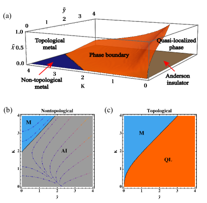
Figure 1: (a) RG phase diagram in the $\tilde{y}$-$K$-$\tilde{\chi}$ space with initial values of $\lambda=\zeta=1$. (b) RG phase diagram in the $\tilde{y}$-$K$ plane at $\tilde{\chi}=0$. (c) RG phase diagram in the $\tilde{y}$-$K$ plane at $\tilde{\chi}=0.1$. The blue regions denote the (critical) metal phase in (b,c), the grey region in (b) is the Anderson localized (AI) phase with $\tilde{\chi}=0$, and the red region in (c) is the quasi-localized (QL) phase with $\tilde{\chi}\neq 0$. In the phase diagram, the metal and quasi-localized phases are separated by a phase boundary (red surface in (a)). The phase diagram with other initial values of $\lambda$ and $\zeta$ takes the same structure as (a) except for the emergence of an unphysical stong-coupling phase in larger $\tilde{y}$ regions [36].

RG phase diagram.—In the 4D parameter space with $\tilde{y}<\infty$, the RG equations have a stable fixed point and a stable fixed region in an infrared limit ($l\rightarrow\infty$), which characterize quasi-localized and metal phases at $\tilde{\chi}\neq 0$, respectively. At the stable fixed point, $K=\zeta=0$, $\tilde{y}^{2}\tilde{B}_{x}=2$ and $\tilde{y}^{2}\tilde{B}_{y}=0$, around which the conductivity equations reduce to $\mathrm{d}\ln\sigma_{x}/\mathrm{d}l=-2$ and $\mathrm{d}\ln\sigma_{y}/\mathrm{d}l=0$. Thus, all parameter points that contract into the fixed point are in the same thermodynamic phase with vanishing $\sigma_{x}$ and finite $\sigma_{y}$; the fixed point characterizes the quasi-localized phase with $\sigma_{x}=0$ and $\sigma_{y}\neq 0$. The values of $\tilde{\chi}$ and $\tilde{y}$ at the fixed point are determined by $-1+13\tilde{\chi}^{2}-10\tilde{\chi}^{4}=0$ and $\tilde{y}=\sqrt{2/3}(1+\tilde{\chi}^{2})^{2}/|\tilde{\chi}|$.

The stable fixed region is given by a condition of $\tilde{y}=0$, $2<K$, and $\tilde{\chi}=\infty$, around which the RG equations can be linearized; $\mathrm{d}\tilde{y}/\mathrm{d}l=(2-K)\tilde{y}$, $\mathrm{d}\tilde{\chi}/\mathrm{d}l=\tilde{\chi}$, $\mathrm{d}K/\mathrm{d}l=\mathrm{d}\zeta/\mathrm{d}l=0$. All parameter points that contract into the fixed region are in the (critical) metal phase with weak topology. In fact, the fugacity $\tilde{y}$ vanishes, and both $\tilde{B}_{x}$ and $\tilde{B}_{y}$ vanish as $1/\tilde{\chi}^{6}$ toward the fixed region, yielding $\mathrm{d}\ln\sigma_{\mu}/\mathrm{d}l=0$ and $\sigma_{\mu}\neq 0$ for $\mu=x,y$ in the infrared (IR) limit.

The RG equations also have a saddle fixed point which characterizes criticality of a quantum phase transition between the quasi-localized and metal phases. At the fixed point, $\zeta=0$, $K\equiv K_{c}=3/4$, $\tilde{y}^{2}\tilde{B}_{x}=3/2$ and $\tilde{y}^{2}\tilde{B}_{y}=-1/2$. A scaling dimension of a relevant scaling variable is evaluated as $0.819$. Fig. 1 shows a RG phase diagram subtended by $K$, $\tilde{\chi}$ and $\tilde{y}$ with intial values of isotropic conductivity and Gade constant ($\zeta=\lambda=1$). When $\tilde{\chi}\neq 0$, the RG phase diagram consists of metal phase with $\sigma_{\mu}\neq 0$ ($\mu=x,y$) and quasi-localized phase with $\sigma_{x}=0$ and $\sigma_{y}\neq 0$ (Figs. 1(a,c)). From the above scaling analysis, a universal critical exponent of the quantum phase transition between the two phases is evaluated as $1/0.819\approx 1.22$.

Numerical study.— The RG study predicts that the quasi-localized phase emerges next to the (critical) metal phase in a phase diagram for chiral symmetry class with weak topology. A previous numerical study showed this in 3D models with weak topology [25]. Here we study a 2D model in chiral unitary class with fninite weak topological index, and demonstrate the emergence of the quasi-localized phase next to the critical metal phase. We study a $2L_{x}\times 2L_{y}$ square-lattice generalization of the Su-Schrieffer-Heeger model [37];

$$H=\sum_{x,y}\left(t_{x,y}^{(x)}c_{x+1,y}^{\dagger}c_{x,y}+t_{x,y}^{(y)}c_{x,y+1}^{\dagger}c_{x,y}\right)+\text{h.c.},$$ (12)

with integers $x=1,2,\cdots,2L_{x}$ and $y=1,2,\cdots,2L_{y}$, and staggered hopping terms $t_{x,y}^{(x)}=(t_{x}+t)/2+(-1)^{x+y}(t_{x}-t)/2+\epsilon_{x,y}(1-(-1)^{x})/2$ and $t_{x,y}^{(y)}=(t_{y}+t)/2+(-1)^{x+y}(t_{y}-t)/2$. $\epsilon_{x,y}$ is a complex number, whose real and imaginary parts are distributed uniformly in a range of $[-W/2,W/2]$. $W$ stands for the disorder strength of the model. The unit cell of the model has four inequivalent sublattices; 1 (even $x$, even $y$), 2 (odd $x$ and odd $y$), 3 (odd $x$, even $y$), and 4 (even $x$ and odd $y$). They are divided into two sublattice groups; (1,2) and (3,4). The model comprises hoppings between the two groups, having the chiral symmetry, $\sigma_{3}H\sigma_{3}=-H$, where $\sigma_{3}$ takes $+1$ for one of the two sublattice groups and $-1$ for the other. Finite $\epsilon_{x,y}$ breaks the time-reversal symmetry, and the model belongs to the chiral unitary class. Due to the chiral symmetry, $H$ can be in a block-off-diagonal form, $H=\sigma_{+}\otimes h+\sigma_{-}\otimes h^{\dagger}$, where a non-Hermitian matrix $h$ defines the one-dimensional weak topological indices $\nu_{\mu}$ $(\mu=x,y)$ [36, 38, 13, 39]. $\nu_{\mu}$ is given by a difference between a number $N_{\nu,+}$ of positive Lyapunov exponents (LEs) of $h$ along $\mu$ and a number $N_{\nu,-}$ of negative LEs; $\nu_{\mu}=(N_{\nu,+}-N_{\nu,-})/(2L)$ [25, 40, 36]. Statistical symmetries of an ensemble of disordered $h$ require the weak topological index along $\mu$ to be zero for $t_{\mu}=t$ ($\mu=x,y$) [36, 25]. To study a phase diagram of disordered $H$ with $\nu_{y}\neq 0$ and $\nu_{x}=0$, we set the hopping parameters as $(t_{x},t_{y})=t(1,1.5)$. This corresponds to the NLSM with $\vec{\chi}=(0,\chi_{y})$.

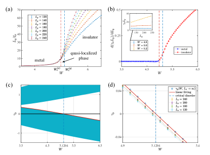
Figure 2: (a) Normalized localization length along $x$, $L_{y}/\xi_{x}\equiv\gamma_{x}L_{y}$, as a function of disorder strength $W$. (b) $\mathrm{d}(\gamma_{x}L_{y})/\mathrm{d}L_{y}$ is shown as a function of $W$ around $W=5$. $\mathrm{d}(\gamma_{x}L_{y})/\mathrm{d}L_{y}$ for each $W$ is determined from a linear fitting of the data from system sizes $L_{y}=120\sim 240$. Inset of (b) shows $\gamma_{x}L_{y}$ as a function of $L_{y}$ for typical $W=4.8,~{}5.0,~{}5.2$. The critical disorder $W^{(c)}_{x}$ (red dashed lines) is a point below which $\mathrm{d}(\gamma_{x}L_{y})/\mathrm{d}L_{y}$ becomes zero; $W^{(c)}_{x}\approx 4.979$. (c) Distribution of the LEs of $h$ along $y$ as a function of $W$ ($L_{x}=240$). With large $L_{x}$, the LEs of $h$ form two continuous bands (blue colored bands) for $W\gtrsim 3.5$. The lower continuous band covers zero in the metal phase ($W<W^{(c)}_{y}=5.12...$); the localization length along $y$ is divergent in the metal phase. (d) The largest LE in the lower continuous band as a function of $W$ for different $L_{x}$. From a linear fitting, we determine an extrapolated value of the largest LE in the limit of $L_{x}=\infty$ as a function of $W$ (red solid line). The critical disorder strength $W^{(c)}_{y}$ (blue dashed lines) is a point where the extrapolated largest LE crosses zero; $W^{(c)}_{y}\approx 5.1204$.

The emergence of the quasi-localized phase is confirmed by transfer matrix calculations  [41, 42, 43]. A localization length $\xi_{x}$ of $H$ along $x$ is calculated with quasi-one-dimensional geometry (Q1D), $L_{x}\gg L_{y}$. The LEs of $h$ along $y$ are calculated with $L_{y}\gg L_{x}$. The LEs of $H$ are a union of the LEs of $h$ and their opposite numbers [25, 36], so a localization length $\xi_{y}$ of $H$ along $y$ is the smallest absolute value of the LEs of $h$. Fig. 2(a,c) show that the model undergoes transitions from metal to localized phases in a region of $4<W<6$. In the metal phase, $\xi_{y}$ is divergent; the lower half of the LEs of $h$ along $y$ forms a continuous band in $L_{x}\rightarrow\infty$ [42], and the band covers zero in the metal phase. $\xi_{x}/L_{y}$ stays invariant for increasing $L_{y}$ in the metal phase. In the localized phase, $\xi_{y}$ is finite in the thermodynamic limit, while $\xi_{x}/L_{y}$ decreases for increasing $L_{y}$, indicating that $\xi_{x}$ is also finite in the thermodynamic limit $L_{y}\rightarrow\infty$. We determine a critical disorder strength $W^{(c)}_{x}$ for the change of $\xi_{x}/L_{y}$, and a critical disorder strength $W^{(c)}_{y}$ for the change of $\xi_{y}$. Note also that $\nu_{y}>0$ for $W<W^{(c)}_{y}$ and $\nu_{y}=0$ for $W>W^{(c)}_{y}$. From fitting analyses [36, 25, 41, 44], the two critical disorder strengths are evaluated as $W^{(c)}_{x}=4.979\pm 0.016$ and $W^{(c)}_{y}\approx 5.1204\pm 0.002$ at $(t_{x},t_{y})=t(1,1.5)$. A discrepancy between the two is about $3\%$ of the critical values, and it is much greater than the error bar of the fittings. This suggests a phase diagram with (i) critical metal phase with $\nu_{y}>0$ ($W<W^{(c)}_{x}$), (ii) quasi-localized phase with $\nu_{y}>0$ ($W^{(c)}_{x}<W<W^{(c)}_{y}$), and (iii) Anderson localized phase with $\nu_{y}=0$ ($W^{(c)}_{y}<W$). In the quasi-localized phase, $\nu_{y}>0$, $\xi_{y}$ is divergent and $\xi_{x}$ is finite in the thermodynamic limit.

Summary.—Emergent spatial anisotropy in transports has been a subject of intense debate during the last decades [45], while it has been widely believed that the conductivity along all the spatial directions vanishes simultaneously at metal-insulator transitions [29, 46]. We study a field theory with a weak topological term and clarify that the interplay between weak topology and disorder induces the proliferation of spatially-polarized vortex-antivortex pairs near the metal-insulator transition in chiral symmetry classes. This results in the universal emergence of the quasi-localized phase that shows the extreme spatial anisotropy in its transport property. We argue the mechanism by RG analyses of the NLSM for the 2D chiral unitary class with weak topology. The RG phase diagram shows that the NLSM with $\vec{\chi}=(0,\chi_{y})$ undergoes a second-order phase transition from the metal phase with $\sigma_{x}\neq 0$ and $\sigma_{y}\neq 0$ to quasi-localized phase with $\sigma_{x}=0$ and $\sigma_{y}\neq 0$. The RG analysis estimates the critical exponent of the quantum phase transition as $\nu\approx 1.22$ in the 2D chiral unitary class.

Acknowledgement.— We thanks Siyu Pan, Lingxian Kong, Tong Wang, Kohei Kawabata, Xunlong Luo, and Tomi Ohtsuki for discussions and comments. The work was supported by the National Basic Research Programs of China (No. 2019YFA0308401) and the National Natural Science Foundation of China (No. 11674011 and No. 12074008).

Supplement for “Topological effect on the Anderson transition in chiral symmetry classes”

Supplemental Material of “Topological Effect on the Anderson transition in chiral symmetry classes” Pengwei Zhao Zhenyu Xiao Yeyang Zhang Ryuichi Shindou

Contents

1. I The effect of weak topological term
   1. I.1 Nonlinear sigma model
   2. I.2 Topological defects
   3. I.3 Weak topological term
   4. I.4 Effect of the weak topological term on Anderson transition
2. II Dual theory for 2D AIII nonlinear sigma model
3. III Renormalization of the dual theory
   1. III.1 Approximations
   2. III.2 Momentum-space decomposition
   3. III.3 Calculations of renormalizations
      1. III.3.1 Correlation functions
      2. III.3.2 Integral over $\mathbb{CP}^{N-1}$ elements
      3. III.3.3 Calculation of $\left\langle S_{y}\right\rangle$ and renormalization of fugacity $y$
      4. III.3.4 Calculation of $\left\langle S_{y}^{2}\right\rangle$ and renormalization of $\sigma_{x},\sigma_{y},c_{x},c_{y}$
   4. III.4 $N=1$ case: commensurate-incommensurate transition
   5. III.5 $N\to 0$ case: Anderson transition and quasi-localization
   6. III.6 fixed points at finite $\tilde{y}$
   7. III.7 fixed points at $\tilde{y}=0$
4. IV Numerical simulation
   1. IV.1 Tight-binding models
   2. IV.2 Transfer matrix

I The effect of weak topological term

I.1 Nonlinear sigma model

The interplay between disorder and topology gives rise to a novel quantum interference effect in physical systems. A recent numerical work studied the Anderson transition in chiral symmetry classes with a weak topology and revealed that one-dimensional weak topological index (“winding number”) induces an emergent quasi-localized phase between diffusive metal and Anderson insulator phases. The intermediate phase has a divergent localization length in a spatial direction with the non-zero winding number, and finite localization lengths along the other spatial directions. In the quasi-localized phase, the conductance along the divergent length remains finite with a non-Ohmic scaling in the thermodynamic limit, while the conductance along the other directions vanishes exponentially. The physical mechanism of the emergent quasi-localized phase is unknown at this moment. In the present paper, we carry out a field-theoretical study of Anderson localization in chiral classes with the weak topological term. We clarify that the interference effect due to the one-dimensional weak topological index results in the emergence of the quasi-localized phase.

Low-energy and long-wavelength behaviors of diffusion in disordered systems are described by a nonlinear sigma model (NLSM). The effective theory is formulated in terms of either a supersymmetry, Keldysh equation approach, or a replica method. In this paper, we use the replica formulation, where a partition function $Z$ for the $d$-dimensional chiral symmetric systems is described by the following NLSM,

$$Z =\int\mathrm{D}[Q]e^{-S},$$

$$S =-\int\frac{\mathrm{d}^{d}r}{8\pi}\sum_{\mu=1}^{d}\left[\sigma_{\mu}\operatorname{Tr}(Q^{-1}\partial_{\mu}Q)^{2}+c_{\mu}\operatorname{Tr}^{2}(Q^{-1}\partial_{\mu}Q)-\chi_{\mu}\operatorname{Tr}(Q^{-1}\partial_{\mu}Q)\right],$$ (S1)

with $\mu=1,2,\cdots,d$. The field variable of the NLSM is a $N\times N$ matrix field $Q$, where $N$ is a number of replicated fermion fields in the replica method. $\sigma_{\mu}$ stands for a physical conductivity along $\mu$-direction. $c_{\mu}$ is a Gade constant that also has a dependence on spatial direction in general. A vector $(\chi_{1},\chi_{2},\dots,\chi_{d})$ quantifies the one-dimensional weak topology. The direction of the vector specifies the one-dimensional topological direction. The norm of the vector quantifies the winding number along the topological direction averaged over the other directions. The topological term can be derived from a lattice model in the chiral class with weak band topology [13]. In the following, a summation over repeated index $\mu$ is always assumed.

Table 1 enumerates symmetries of the field variable $Q$ and its low-energy manifolds (“Goldstone” manifolds) in the three chiral symmetry classes. As a common feature in the chiral classes, the low-energy manifolds have a $\mathrm{U}(1)$ subgroup symmetry. Due to this $\mathrm{U}(1)$ subgroup symmetry, perturbative $\beta$-functions of the NLSM are zero for the chiral symmetry classes [34, 33], while the $\mathrm{U}(1)$ subgroup part of the $Q$ field accommodates vortex excitations. Accordingly, it has been argued that the Anderson transition in the chiral classes is driven by spatial proliferation of the vortex excitations of the $Q$-field [20, 44]. It has been also argued that strong topological terms with quantized topological number hinder the vortex proliferation through destructive quantum interference effect [20]. Nonetheless, quantum interference effect due to the one-dimensional weak topological index has not been discussed previously, and associated consequences on localized phase proximate to metal phase remains unclear. We will discuss the quantum interference effect due to the weak topological term, and clarify that the interference alters the localized phase into the quasi-localized phase.

Symmetry class	Goldstone manifold	Restriction
AIII	$\mathrm{U}(N)$	No restriction
BDI	$\mathrm{U}(N)/\mathrm{Sp}(N)$	$Q=CQ^{\mathrm{T}}C,C^{2}=1,C^{\mathrm{T}}=-C$
CII	$\mathrm{U}(N)/\mathrm{O}(N)$	$Q=Q^{\mathrm{T}}$

Supplementary Table 1: Goldstone manifolds of the field variable $Q$ and symmetries of the $Q$ field. The matrix $C$ is an arbitrary antisymmetric matrix with condition $C^{2}=1$.

I.2 Topological defects

For further discussion, an exact definition of topological defects is necessary. The vortex excitations can be often introduced as saddle-point configurations of the NLSM, that have a discontinuity around a lower dimensional area. Taking a functional derivative of Eq.(S1), $S=S_{\text{cond}}+S_{\text{Gade}}+S_{\text{top}}$, one obtain the saddle-point equation. Define a small variation of $Q$ as $Q\rightarrow Q+\delta Q$ and its ivertese $Q^{-1}\rightarrow Q^{-1}-Q^{-1}\delta QQ^{-1}$. One can check the relation holds

$$\left(Q^{-1}-Q^{-1}\delta QQ^{-1}\right)\left(Q+\delta Q\right)=1+Q^{-1}\delta Q-Q^{-1}\delta Q+{\cal O}(||\delta Q||^{2})=1.$$ (S2)

A small matrix $\delta Q$ means $||\delta Q||^{2}\equiv\operatorname{Tr}\left(\delta Q^{\dagger}\delta Q\right)\ll 1$. Now, we put this replacement into Eq. S1 and omit the 2nd order terms of $\delta Q$. For example,

$$\delta\operatorname{Tr}\left(Q^{-1}\partial_{\mu}Q\right)=\operatorname{Tr}\left(-Q^{-1}\delta QQ^{-1}\partial_{\mu}Q+Q^{-1}\partial_{\mu}\delta Q\right).$$ (S3)

The topological term $S_{\text{top}}$ gives

$$\delta S_{\text{top}}=-\int\frac{\mathrm{d}^{d}r}{8\pi}\,\chi_{\mu}\operatorname{Tr}\left[\left(Q^{-1}\partial_{\mu}QQ^{-1}+\partial_{\mu}Q^{-1}\right)\delta Q\right].$$ (S4)

The Gade term $S_{\text{Gade}}$ yields

$$\begin{gathered}\delta S_{\text{Gade}}=\int\frac{\mathrm{d}^{d}r}{8\pi}\,2c_{\mu}\left(\operatorname{Tr}\left(Q^{-1}\partial_{\mu}Q\right)\operatorname{Tr}\left(Q^{-1}\partial_{\mu}QQ^{-1}\delta Q\right)+\operatorname{Tr}\left(\partial_{\mu}Q^{-1}\partial_{\mu}Q\right)\operatorname{Tr}\left(Q^{-1}\delta Q\right)\right.\\ \left.+\operatorname{Tr}\left(Q^{-1}\partial_{\mu}^{2}Q\right)\operatorname{Tr}\left(Q^{-1}\delta Q\right)+\operatorname{Tr}\left(Q^{-1}\partial_{\mu}Q\right)\operatorname{Tr}\left(\partial_{\mu}Q^{-1}\delta Q\right)\right).\end{gathered}$$ (S5)

The conductivity term $S_{\text{cond}}$ can be written in the following form

$$S_{\text{cond}}=-\int\frac{\mathrm{d}^{d}r}{8\pi}\sigma_{\mu}\operatorname{Tr}\left(Q^{-1}\partial_{\mu}Q\right)^{2}=\int\mathrm{d}^{3}r\,\sigma_{\mu}\operatorname{Tr}\left(\partial_{\mu}Q^{-1}\partial_{\mu}Q\right),$$ (S6)

whose variation is given by

$$\delta S_{\text{cond}}=\int\mathrm{d}^{3}r\,\sigma_{\mu}\operatorname{Tr}\left[\left(Q^{-1}\partial_{\mu}^{2}QQ^{-1}-\partial_{\mu}^{2}Q^{-1}\right)\delta Q\right].$$ (S7)

The stationary condition $\delta S=0$ gives a saddle-point equation

$$\begin{gathered}\sigma_{\mu}\left(Q^{-1}\partial_{\mu}^{2}QQ^{-1}-\partial_{\mu}^{2}Q^{-1}\right)+2c_{\mu}\operatorname{Tr}\left(Q^{-1}\partial_{\mu}Q\right)\left(Q^{-1}\partial_{\mu}QQ^{-1}+\partial_{\mu}Q^{-1}\right)\\ +2c_{\mu}\left[\operatorname{Tr}\left(\partial_{\mu}Q^{-1}\partial_{\mu}Q\right)+\operatorname{Tr}\left(Q^{-1}\partial_{\mu}^{2}Q\right)\right]Q^{-1}+\chi_{\mu}\left(Q^{-1}\partial_{\mu}QQ^{-1}+\partial_{\mu}Q^{-1}\right)=0.\end{gathered}$$ (S8)

As $\partial QQ^{-1}+Q\partial Q^{-1}=\partial(QQ^{-1})=0$, the stationary condition is equivalent to

$$2\sigma_{\mu}\partial_{\mu}\left(Q\partial_{\mu}Q^{-1}\right)+2c_{\mu}\partial_{\mu}\left(\operatorname{Tr}\left(Q\partial_{\mu}Q^{-1}\right)\right)=0$$ (S9)

For $N=1$, $\mathrm{U}(1)$ field is given by $Q=e^{i\phi}$, and the saddle-point equation reduces to the Poisson equation

$$(\sigma_{\mu}+c_{\mu})\partial_{\mu}^{2}\phi=0.$$ (S10)

With reduced coordinates $\bar{r}_{\mu}\equiv r_{\mu}/\sqrt{\sigma_{\mu}+c_{\mu}}$, the saddle-point equation is

$$\bar{\nabla}^{2}\phi=0.$$ (S11)

Solutions of the saddle-point equation can generally have a phase winding around a $(d-2)$-dimensional vortex core

$$\oint_{C}\mathrm{d}\bm{\bar{r}}\cdot\bm{\bar{\bm{\nabla}}}\phi=2\pi\eta.$$ (S12)

When a one-dimensional loop $C$ encircles the core, $\eta$ on the right-hand side takes an integer value (vortex charge).

For $N\neq 1$, $Q$ has unit complex numbers $e^{i\phi_{a}}$ as its eigenvalues, $Q=\sum^{N}_{a=1}\ket{p_{a}}e^{i\phi_{a}}\bra{p_{a}}$. Here $\ket{p_{a}}$ is a normalized column vector, $\braket{p_{a}}{p_{a}}=1$, belonging to the complex projective space $\mathbb{CP}^{N-1}$, real projective space $\mathbb{RP}^{N-1}$, and quaternion projective space $\mathbb{HP}^{N/2-1}$ for chiral unitary, chiral symplectic, and chiral orthogonal classes respectively. Let us consider a uniform $Q$-field configuration, $Q({\bm{r}})=\mathds{1}$, add a vortex exictation. Around the vortex core, one of the eigenvalues has the phase winding, while all the others are close to unit,

$$Q({\bm{r}})=\mathds{1}+\ket{p({\bm{r}})}(e^{i\phi({\bm{r}})}-1)\bra{p({\bm{r}})}.$$ (S13)

Namely, $\phi$ is a solution of $\bar{\nabla}^{2}\phi=0$ with the phase winding around the core; Eq (S12), and $\ket{p({\bm{r}})}$ is an eigenvector for the eigenvalue with the phase winding. $\ket{p({\bm{r}})}$ generally depends on the spatial coordinate ${\bm{r}}$. A $Q$-field configuration with multiple vortices at ${\bm{r}}_{1},\cdots,{\bm{r}}_{n}$ can be also given by the same ansatz, Eq. (S13), where $\phi$ has phase windings around these cores, and $\ket{p({\bm{r}}_{i})}$ and $\ket{p({\bm{r}}_{j})}$ are generally different from one another because of the ${\bm{r}}$-dependence of $\ket{p({\bm{r}})}$. We assume that an eigenvector $\ket{p({\bm{r}})}$ is slowly varying in the space coordinate compared to a typical size of vortex cores. In fact, the ansatz Eq. (S13) with ${\bm{r}}$-independent $\ket{p}$ can be also introduced as a solution of the saddle-point equation for the isotropic case ($\sigma_{1}=\sigma_{2}=\cdots=\sigma_{d}$, $c_{1}=c_{2}=\cdots=c_{d}$) as well as an anisotropic case with a fixed ratio between conductivity and Gade constant ($\sigma_{1}/c_{1}=\sigma_{2}/c_{2}=\cdots=\sigma_{d}/c_{d}$).

The configuration with a vortex is discontinuous at a vortex core with a non-zero commutation of the second-order derivative of the phase $\phi$, $[\bar{\partial}_{\mu},\bar{\partial}_{\nu}]\phi\neq 0$ for some $\mu\neq\nu$. A line integral along a closed loop $C$ can be written as a surface integral over a region $\Gamma$

$$\oint_{C}\mathrm{d}\bm{\bar{r}}\cdot\bm{\bar{\bm{\nabla}}}\phi=\iint_{\Gamma}\mathrm{d}\bm{\bar{\Gamma}}\cdot\bm{\bar{\nabla}}\times\bm{\bar{\nabla}}\phi=2\pi\eta,$$ (S14)

with $C=\partial\Gamma$. The surface integral yields a nonzero value if the vortex core penetrates through the surface. The property associates $\bm{\bar{\nabla}}\times\bm{\bar{\nabla}}\phi$ with a Dirac delta function in a way that depends on the spatial dimension.

2D cases. For $d=2$, the vortex core is a 0-dimensional point. The commutator is a two-dimensional delta function at the core,

$$[\bar{\partial}_{x},\bar{\partial}_{y}]\phi=2\pi\eta\delta^{2}(\bm{\bar{r}}-\bm{\bar{r}}_{0}).$$ (S15)

Equivalently,

$$[\partial_{x},\partial_{y}]\phi=2\pi\eta\delta^{2}(\bm{r}-\bm{r}_{0}),$$ (S16)

with $\bar{r}_{\mu}=r_{\mu}/\sqrt{\sigma_{\mu}+c_{\mu}}$. $\phi$ that satisfies Eq. S11 and Eq. S16 is given by

$$\phi=\eta\arctan\left(\frac{\overline{y}-\overline{y}_{0}}{\overline{x}-\overline{x}_{0}}\right).$$ (S17)

3D cases. For $d=3$, the vortex core takes the form of a one-dimensional line. The line can form a closed loop. The vortex loop can be parameterized as $\bm{l}(s)$ with a parameter $s\in[-1,1]$. For example, a circle in the $xy$-plane is

$$l_{x}=R\cos(\pi s),\quad l_{y}=R\sin(\pi s),\quad l_{z}=0.$$ (S18)

A straight line along $(u_{x},u_{y},u_{z})$ from $(x_{0},y_{0},z_{0})$ is

$$l_{x}=x_{0}+u_{x}\arctan(s),\quad l_{y}=y_{0}+u_{y}\arctan(s),\quad l_{z}=z_{0}+u_{z}\arctan(s).$$ (S19)

Given such parameterizations of a vortex line $\bm{\bar{l}}(s)$, the non-zero $\bar{\bm{\nabla}}\times\bar{\bm{\nabla}}$ is defined by

$$\epsilon_{ijk}\bar{\partial}_{j}\bar{\partial}_{k}\phi=2\pi\eta\int\mathrm{d}s\,\frac{\mathrm{d}\bar{l}_{i}}{\mathrm{d}s}\delta^{3}(\bm{\bar{r}}-\bm{\bar{l}}).$$ (S20)

or

$$\epsilon_{ijk}\partial_{j}\partial_{k}\phi=2\pi\eta\int\mathrm{d}s\,\frac{\mathrm{d}l_{i}}{\mathrm{d}s}\delta^{3}(\bm{r}-\bm{l}).$$ (S21)

Importantly, the form of the non-zero commutation of the second-order spatial derivative is not affected by the anisotropies of conductivity and Gade constant.

I.3 Weak topological term

The topological term in Eq. (S1) is associated with weak topology in the topological band theory, and it is quantified by a vector $\vec{\chi}\equiv\bm{\chi}=(\chi_{1},\chi_{2},\cdots,\chi_{d})$ in the NLSM. In this section, we briefly review the weak topology. Topology in the field theory is defined as the homotopy group of the field variable $Q$ on the $d$-dimensional space, where $Q$ is regarded as a map from the coordinate space $\mathbb{R}^{d}$ to the low-energy (“Goldstone”) manifold $G$. With some boundary conditions, the coordinate space $\mathbb{R}^{d}$ becomes a compact space. For a fixed boundary condition $Q(|{\bm{r}}|=\infty)\equiv 1$, $\mathrm{R}^{d}$ is compactified into $\mathrm{SO}(d)$, $\mathrm{R}^{d}\simeq\mathrm{SO}(d)$. For a periodic boundary condition, $\mathrm{R}^{d}\simeq\mathrm{U}(1)^{d}$. If two maps, $Q_{1}$ and $Q_{2}$, are continuously transformed into each other, they belong to an equivalent class. Inequivalent classes form homotopy group $\pi(\mathrm{R}^{d},G)$, and an algebra of the group defines the strong topology of the field variable $Q$ in $\mathrm{R}^{d}$. A weak topology is associated with a homotopy group of the field variable in a lower dimensional subspace of $\mathrm{R}^{d}$. For example, $Q$ as a function of one of the coordinates, say $r_{1}$ with ${\bm{r}}\equiv(r_{1},r_{2},\dots,r_{d-1},r_{d})$, can be regarded as a map from $\mathbb{R}$ to $G$. For both fixed and periodic boundary conditions, $\mathbb{R}\simeq U(1)$, where the map defines another homotopy group, $\pi(\mathrm{U}(1),G)$. For class AIII, $G=\mathrm{U}(N)$ where the homotopy group in the one-dimensional subspace is classified by an integer;

$$\pi(\mathrm{U}(1),\mathrm{U}(N))=\pi(\mathrm{U}(1),\mathrm{U}(1)\times\mathrm{SU}(N))=\pi(\mathrm{U}(1),\mathrm{U}(1))\times\pi(\mathrm{U}(1),\mathrm{SU}(N))=\mathbb{Z}\times 1=\mathbb{Z}.$$ (S22)

The integer manifests itself in the topological term in the NLSM,

$$\int\frac{dr_{1}}{2\pi i}\operatorname{Tr}(Q^{-1}\partial_{r_{1}}Q)=\mathbb{Z}.$$ (S23)

Note that the NLSM with the topological term can be derived from a lattice model in the chiral class with a weak topological index of the topological band theory.

I.4 Effect of the weak topological term on Anderson transition

The Anderson transition in chiral symmetry classes without the topological term has been studied previously, and the study shows that it is driven by the spatial proliferation of the vortices of the $Q$-field configuration [20, 44]. The topological term $S_{\text{top}}$ gives a complex phase factor to the $Q$-field configuration with the vortices. The phase factor induces a quantum interference effect in the configuration space of the $Q$-field, rendering the Anderson transition in chiral symmetry classes into a unique quantum phase transition in a way that depends on the spatial dimension.

2D cases. To see how the quantum interference effect appears in $d=2$, let us evaluate the topological term in the presence of a pair of vortex and antivortex,

$$Q_{\bm{m}}({\bm{r}})=\mathds{1}+\ket{p({\bm{r}})}\left(e^{i\phi_{\bm{m}}({\bm{r}})}-1\right)\bra{p({\bm{r}})},\quad\phi_{\bm{m}}=\arctan\left(\frac{y-y_{1}}{x-x_{1}}\right)-\arctan\left(\frac{y-y_{2}}{x-x_{2}}\right),\quad\bm{m}=r_{2}-r_{1}.$$ (S24)

A relative coordinate between vortex at ${\bm{r}}_{1}$ and antivortex at ${\bm{r}}_{2}$ can be regarded as dipole vector $\bm{m}$ of the pair. Substituting $Q_{\bm{m}}$ into the action $S_{\text{top}}$, one can see that the topological term gives a pure imaginary number that depends on the direction of the dipole vector,

$$S_{\text{top}}[Q_{\bm{m}}]=i\eta\chi_{\mu}\int\frac{\mathrm{d}^{2}r}{8\pi}\partial_{\mu}\phi_{\bm{m}}=\frac{i}{4}\eta\big{(}\chi_{x}m_{y}-\chi_{y}m_{x}\big{)}.$$ (S25)

Note that the other parts of the action are real-valued. Thus, when the dipole has a finite angle against $(\chi_{x},\chi_{y})$ in the 2D plane, such dipole configurations with different angles show destructive interference in the partition function. In a simpler case where a ratio between conductivity and Gade constant $\sigma_{\mu}/c_{\mu}$ is independent of the spatial direction $\mu$, $S_{\rm cond}+G_{\rm Gade}$ with the dipole depends only on $|{\bm{m}}|$ in the reduced coordination $\overline{r}_{\mu}\equiv r_{\mu}/{\sqrt{\sigma_{\mu}+c_{\mu}}}$. Thereby, the dipole configurations with same $|{\bm{m}}|$ and different angles against $(\chi_{x},\chi_{y})$ show the destructive interference. The destructive interference becomes prominent for larger $|{\bm{m}}|$ and $|\chi_{\mu}|$. On the other hand, dipoles that are parallel to $(\chi_{x},\chi_{y})$ are free from the interference effect, and naturally dominate the partition function around the Anderson transition. Accordingly, in the presence of the topological term, disordered metals in the chiral classes undergo a spatially anisotropic proliferation of vortices where pairs of vortex and antivortex tend to be polarized along $(\chi_{x},\chi_{y})$ (Fig. S1). The Proliferation of the polarized pairs of vortices makes spatial correlations of the $Q$-field to be strongly disordered along $(-\chi_{y},\chi_{x})$ direction while leaving weakly disordered the spatial correlation along $(\chi_{x},\chi_{y})$ direction. The feature is consistent with the emergent quasi-localized phase with divergent localization length along the topological direction, $(\chi_{x},\chi_{y})$, and finite localization length along the other direction, $(-\chi_{y},\chi_{x})$.

Figure S1: Schematic pictures of a spatial proliferation of vortex-antivortex pairs in 2D space, (a) in the absence of weak topology $\vec{\chi}=0$, (b) in the presence of weak topology $\vec{\chi}\neq 0$. Solid and hollow circles represent vortex and antivortex, respectively, and dashed lines are branchcuts for vortex-antivortex pairs. For given locations of vortices and antivortices in the 2D space, the partition function $Z$ depends neither on the choice of the branch cuts nor on specific pairings of vortices and antivortices.

3D cases. For $d=3$, let us evaluate the topological term in the presence of a closed loop $\Gamma$ of the vortex line,

$$Q_{\Gamma}({\bm{r}})=\mathds{1}+\ket{p({\bm{r}})}\left(e^{i\phi_{\Gamma}({\bm{r}})}-1\right)\bra{p({\bm{r}})},\quad\epsilon_{ijk}\partial_{j}\partial_{k}\phi_{\Gamma}({\bm{r}})=2\pi\eta\int^{1}_{-1}ds\!\ \frac{dl_{i}}{ds}\!\ \delta^{3}\left({\bm{r}}-{\bm{l}}(s)\right).$$ (S26)

Here the loop $\Gamma$ is parameterized by $s\in[-1,1]$ as ${\bm{l}}(s)\equiv\left(l_{x}(s),l_{y}(s),l_{z}(s)\right)$ with ${\bm{l}}(-1)={\bm{l}}(1)$. A substitution into $S_{\rm top}$ shows that the topological term is proportional to an area of the closed loop projected onto a plane perpendicular to $(\chi_{x},\chi_{y},\chi_{z})$;

$$S_{\rm top}[Q_{\Gamma}]=i\eta\chi_{\mu}\int\frac{\mathrm{d}^{3}r}{8\pi}\partial_{\mu}\phi_{\Gamma}=-\frac{i}{4}\eta\!\ \chi_{\mu}\epsilon_{\mu\nu\lambda}\int^{1}_{-1}l_{\nu}\frac{dl_{\lambda}}{ds}\!\ ds.$$ (S27)

The other parts of the action, $S_{\rm cond}+S_{\rm Gade}$, are real, and depend only on the shape of the vortex loop in the simpler case. Thereby, when vortex loops have finite projections onto the plane, the vortex loops with the same shape and different spatial orientations show destructive interference in the partition function. Consequently, the partition function near the Anderson transition in 3D chiral symmetry classes is dominated by those vortex loops that are confined in planes parallel to the topological direction, ($\chi_{x},\chi_{y},\chi_{z}$). Due to this spatial anisotropic proliferation of vortex loops, a localized phase proximate to a metal phase in the chiral classes with finite $|\vec{\chi}|$ is characterized by the peculiar spatial correlation of the $Q$ field; the correlation is strongly disordered within the plane perpendicular to the topological direction and weakly disordered along the topological direction. This correlation is expected to result in a spatially anisotropic transport property as in the quasi-localized phase.

Motivated by these intuitive arguments, we carry out a field-theoretical analysis of Eq. (S1), and show that the topological term indeed changes the nature of the localized phase proximate to the metal phase in chiral symmetry class with finite $\vec{\chi}$. Specifically, our renormalization group analysis demonstrates that Eq. (S1) with finite $\vec{\chi}$ has only two stable fixed points, where one of them has finite conductivity only along the topological direction $\vec{\chi}$ and vanishing conductivity in the other direction, giving a characterization of the quasi-localized phase. The other stable fixed point has finite conductivities along all directions, characterizing a metal phase. We also find a saddle-point fixed point that controls the criticality of a phase transition between these two phases. For simplicity, in this paper, we only focus on the two-dimensional chiral unitary class, while leaving other dimensions and chiral symmetry classes for future study.

II Dual theory for 2D AIII nonlinear sigma model

The field variable $Q$ in the chiral unitary (AIII) class belongs to $\mathrm{U}(N)$, satisfying $Q^{\dagger}Q=\mathds{1}$. The dual transformation can be generalized from the $\mathrm{U}(1)$ case to the $\mathrm{U}(N)$ case. Define a Hermitian matrix $h_{\mu}\equiv-iQ^{-1}\partial_{\mu}Q$ and rewrite $S$ of Eq. S1 in terms of $h_{\mu}$

$$S=\int\frac{\mathrm{d}^{2}r}{8\pi}\sum_{\mu=x,y}\left(\sigma_{\mu}\operatorname{Tr}h_{\mu}^{2}+c_{\mu}\operatorname{Tr}^{2}h_{\mu}+i\chi_{\mu}\operatorname{Tr}h_{\mu}\right).$$ (S28)

When rewriting the integral measure $\mathrm{D}[Q]$ in terms of $\mathrm{D}[h_{\mu}]$, we include $Q$-field configurations with vortex excitations, using a field strength associated with the Hermitian matrix. Specifically, the field strength tensor is given by

$$F_{\mu\nu}\equiv\partial_{\mu}h_{\nu}-\partial_{\nu}h_{\mu}+i[h_{\mu},h_{\nu}].$$ (S29)

When $Q$-field is a smooth function over the spatial coordinate ${\bm{r}}$, the 2nd-order spatial derivatives of $Q$ is commutative, $[\partial_{\mu},\partial_{\nu}]Q=0$, leading to $F_{\mu\nu}=0$.

When $Q$-field configuration includes the vortex excitation, $Q$ around the vortex core takes a form of

$$Q({\bm{r}})=\mathds{1}+\ket{p({\bm{r}})}\left(e^{i\phi({\bm{r}})}-1\right)\bra{p({\bm{r}})},$$ (S30)

where the U(1) phase $\phi({\bm{r}})$ has the quantized phase winding around the core. The loop integral of the spatial gradient of $\phi$ around the core gives the winding number, resulting in a non-zero commutator of the 2nd-order spatial derivatives of the phase,

$$[\partial_{x},\partial_{y}]\phi=2\pi\eta\delta^{2}(\bm{r}-\bm{r}_{0}).$$ (S31)

The integer $\eta$ stands for vorticity and $\bm{r}_{0}$ is the location of the core. This yields a condition for $F_{xy}$

$$F_{xy}=2\pi\eta\delta^{2}(\bm{r}-\bm{r}_{0})\ket{p({\bm{r}})}\bra{p({\bm{r}})}.$$ (S32)

When $Q$-field configurations include $n$ vortices, $\phi$ in Eq. (S30) has vortices at $n$ different spatial points, ${\bm{r}}_{1},\cdots,{\bm{r}}_{n}$. Then, the condition for $F_{xy}$ can be generalized into the $n$-vortices case,

$$F_{xy}=J^{(n)},\quad J^{(n)}=\sum_{i=1}^{n}2\pi\eta_{i}\delta\left(\bm{r}-\bm{r}_{i}\right)\ket{p_{i}}\bra{p_{i}}.$$ (S33)

Namely, $\ket{p_{i}}$ is the eigenvector $\ket{p({\bm{r}})}$ at ${\bm{r}}={\bm{r}}_{i}$, $\ket{p_{i}}\equiv\ket{p({\bm{r}}_{i})}$, and positive (negative) integer $\eta_{i}$ is the vorticity at the $i$-th vortex (antivortex).

The path integral for the paritition function $Z$ in Eq. (S1) can include all the possible multiple-vortices configurations through it integral measure;

$$\int\mathrm{D}[Q]=\sum_{n=0}^{\infty}\frac{\Lambda^{2n}}{n!}\prod_{i=1}^{n}\left(\int\mathrm{D}[p_{i}]\int\mathrm{d}^{2}r_{i}\sum_{\eta_{i}=-\infty}^{+\infty}y_{\eta_{i}}\right)\int\mathrm{D}[h]\,\delta[F_{xy}-J^{(n)}].$$ (S34)

$y_{\eta}$ is fugacity of single vortex with the vorticity $\eta$. $\delta(F_{xy}-J^{(n)})$ imposes the delta function condition for every matrix element of the $N$ by $N$ Hermitian matrix $F_{xy}$. $\Lambda^{-1}$ is a linear dimension of a vortex core size, which plays the role of an infrared cutoff of the theory. A factor of $``n!"$ in the right-hand side is a symmetry factor that takes into account equivalent $n$-vortices configurations. Here we consider that $n$-vortices are spatially separated from each other, and treat $\ket{p_{i}}=\ket{p({\bm{r}}_{i})}$ for different $i$ as independent integral variables; $\prod^{n}_{i=1}\int\mathrm{D}[p_{i}]$. When ${\bm{r}}_{i}$ becomes equal to ${\bm{r}}_{j}$ in the integrals over ${\bm{r}}_{i}$ and ${\bm{r}}_{j}$, $\ket{p_{i}}$ must be identical to $\ket{p_{j}}$ because they are from the same $\ket{p({\bm{r}})}$. Thereby, $\int\mathrm{D}[p_{i}]\int\mathrm{D}[p_{j}]$ reduces to $\int\mathrm{D}[p_{i}]$ for the ${\bm{r}}_{i}={\bm{r}}_{j}$ case. Likewise, a double sum $\sum_{\eta_{i}}\sum_{\eta_{j}}$ reduces to a single sum over $\eta_{m}\equiv\eta_{i}+\eta_{j}$ for the ${\bm{r}}_{i}={\bm{r}}_{j}$ case. Note that the $n=0$ term corresponds to a continuous configuration of the $Q$ field without vortices. For simplicity, let’s define the following notation

$$\int\mathrm{D}[J^{(n)}]\equiv\prod_{i=1}^{n}\left(\int\mathrm{D}[p_{i}]\int\mathrm{d}^{2}r_{i}\sum_{\eta_{i}=-\infty}^{+\infty}y_{\eta_{i}}\right),$$ (S35)

and

$$\int\mathrm{D}[Q]=\int\mathrm{D}[h]\sum_{n=0}^{\infty}\frac{\Lambda^{2n}}{n!}\int\mathrm{D}[J^{(n)}]\delta[F_{xy}-J^{(n)}].$$ (S36)

In terms of the integral measure, the partition function is given by

$$Z=\int\mathrm{D}[Q]e^{-S}=\int\mathrm{D}[h]\sum_{n=0}^{\infty}\frac{\Lambda^{2n}}{n!}\int\mathrm{D}[J^{(n)}]\delta[F_{xy}-J^{(n)}]\exp\left(-S\right).$$ (S37)

The $\delta$ function can be exponentiated in terms of an auxiliary field $\Theta({\bm{r}})$ ($N$ times $N$ Hermitian matrix)

$$Z=\int\mathrm{D}[h]\int\mathrm{D}[\Theta]\sum_{n=0}^{\infty}\frac{\Lambda^{2n}}{n!}\int\mathrm{D}[J^{(n)}]\exp\left[-S-i\int\mathrm{d}^{2}r\,\operatorname{Tr}\left[\Theta({\bm{r}})\left(F_{xy}({\bm{r}})-J^{(n)}({\bm{r}})\right)\right]\right].$$ (S38)

The partition function can be separated into two parts; one is given by an integral over $h$ field, and the other is given by an integral over vortices degrees of freedom. The two integrals lead to an effective action for the auxiliary field $\Theta$,

$$Z=\int\mathrm{D}[\Theta]\,\exp\left(-S_{\text{smooth}}-S_{\text{vortex}}\right),$$ (S39)

$$S_{\text{smooth}}\equiv-\ln\int\mathrm{D}[h]\,\exp\left[-S-i\int\mathrm{d}^{2}r\,\operatorname{Tr}\left(\Theta F_{xy}\right)\right],$$ (S40)

$$e^{-S_{\text{vortex}}} =\sum_{n=0}^{\infty}\frac{\Lambda^{2n}}{n!}\prod^{n}_{i=1}\bigg{(}\int\mathrm{D}[p_{i}]\int\mathrm{d}^{2}{\bm{r}}_{i}\sum^{+\infty}_{\eta_{i}=-\infty}\bigg{)}\exp\left[i2\pi\sum^{n}_{i=1}\eta_{i}\bra{p_{i}}\Theta({\bm{r}}_{i})\ket{p_{i}}\right],$$ (S41)

$$``="\sum_{n=0}^{\infty}\frac{\Lambda^{2n}}{n!}\bigg{(}\int\mathrm{D}[p]\int\mathrm{d}^{2}{\bm{r}}\sum^{+\infty}_{eta=-\infty}e^{i2\pi\eta\bra{p}\Theta({\bm{r}})\ket{p}}\bigg{)}^{n}=\exp\bigg{[}\Lambda^{2}\int\mathrm{D}[p]\int\mathrm{d}^{2}r\!\ \sum^{\infty}_{\eta=-\infty}e^{i2\pi\eta\bra{p}\Theta({\bm{r}})\ket{p}}\bigg{]},$$

or equivalently,

$$S_{\text{vortex}}=-\Lambda^{2}\int\mathrm{D}[p]\int\mathrm{d}^{2}r\!\ \sum^{\infty}_{\eta=-\infty}e^{i2\pi\eta\bra{p}\Theta({\bm{r}})\ket{p}}.$$ (S42)

Note that the multiple integrals over ${\bm{r}}_{i}$ and $\ket{p_{i}}$ for different $i$ in Eq. (S41) are taken in such a way that any double integral over $\ket{p_{i}}$ and $\ket{p_{j}}$ reduces to a single integral $\ket{p_{i}}$ whenever ${\bm{r}}_{i}={\bm{r}}_{j}$ in the integrals over ${\bm{r}}_{i}$ and ${\bm{r}}_{j}$. In this sense, an exponential of Eq. (S42) is not exactly the same as Eq. (S41). For simplicity of presentation, we write $S_{\rm vortex}$ and its associated function $S_{y}$ (see below) as in Eq. (S42), while their exponentials are always defined with the same definition of the multiple integrals as Eq. (S41).

Smooth part. The integral over $h$ field is a partition function from $Q$-field configurations without vortices (‘smooth part’);

$$\begin{gathered}S_{\text{smooth}}=-\ln\int\mathrm{D}[h]\,\exp\left[-\int\frac{\mathrm{d}^{2}r}{8\pi}\sum_{\mu=x,y}\left(\sigma_{\mu}\operatorname{Tr}h_{\mu}^{2}+c_{\mu}\operatorname{Tr}^{2}h_{\mu}+i\chi_{\mu}\operatorname{Tr}h_{\mu}\right)\right.\\ \left.-i\int\mathrm{d}^{2}r\,\operatorname{Tr}\left(\Theta\left(\partial_{x}h_{y}-\partial_{y}h_{x}+i[h_{x},h_{y}]\right)\right)\right].\end{gathered}$$ (S43)

To carry out the Gaussian integral over $h_{\mu}$, use $\mathrm{u}(N)$ Lie algebra, $T^{a}$ ($a=0,1,\cdots,D-1\equiv N^{2}-1)$, as a basis of the $N$ by $N$ Hermitian matrices $h_{\mu}$ and $\Theta$. The Lie algebra $T_{a}$ satisfies

$$\operatorname{Tr}\left(T^{a}T^{b}\right)=\delta_{ab},\quad\sum_{\tilde{a}=1}^{D-1}T_{ij}^{\tilde{a}}T_{kl}^{\tilde{a}}=\delta_{il}\delta_{jk}-\frac{1}{N}\delta_{ij}\delta_{kl},\quad\operatorname{Tr}\left(T^{\tilde{a}}\right)=0,\quad T^{0}=\frac{1}{\sqrt{N}}\mathds{1},$$ (S44)

with a a structure factor constant of the $\mathrm{u}(N)$ Lie algebra,

$$f_{abc}\equiv-i\operatorname{Tr}\left([T^{a},T^{b}]T^{c}\right).$$ (S45)

By expending $h_{\mu}$ and $\Theta$ in terms of the basis,

$$h_{\mu}=\sum^{D-1}_{a=0,1,\cdots}\pi_{\mu}^{a}T^{a},\quad\Theta=\sum^{D-1}_{a=0}\theta^{a}T^{a},$$ (S46)

we have

$$-i\operatorname{Tr}\left[\Theta(\partial_{x}h_{y}-\partial_{y}h_{x}+i[h_{x},h_{y}])\right]=-i\left(\theta^{a}\partial_{x}\pi_{y}^{a}-\theta^{a}\partial_{y}\pi_{x}^{a}-\pi^{a}_{x}\pi^{b}_{y}\theta^{c}f_{abc}\right),$$ (S47)

$$-i\int\mathrm{d}^{2}r\left(\theta^{a}\partial_{x}\pi_{y}^{a}-\theta^{a}\partial_{y}\pi_{x}^{a}-\pi^{a}_{x}\pi^{b}_{y}\theta^{c}f_{abc}\right)=-i\int\mathrm{d}^{2}r\left(\pi_{x}^{a}\partial_{y}\theta^{a}-\pi_{y}^{a}\partial_{x}\theta^{a}-\pi^{a}_{x}\pi^{b}_{y}\theta^{c}f_{abc}\right),$$ (S48)

and

$$\begin{gathered}S_{\text{smooth}}=-\ln\int\mathrm{D}[h]\exp\left[-\int\frac{\mathrm{d}^{2}r}{8\pi}\left[(\sigma_{\mu}+Nc_{\mu}\delta_{a0})\left(\pi^{a}_{\mu}\right)^{2}+i\sqrt{N}\chi_{\mu}\pi_{\mu}^{0}\right]\right]\\ \times\exp\left[-i\int\mathrm{d}^{2}r\left(\pi_{x}^{a}\partial_{y}\theta^{a}-\pi_{y}^{a}\partial_{x}\theta^{a}-\pi^{a}_{x}\pi^{b}_{y}\theta^{c}f_{abc}\right)\right].\end{gathered}$$ (S49)

The Gaussian integral over $h_{\mu}$ can be separated into the integral over the U(1) part $\pi^{0}$ and the integral over the SU($N$) part $\pi^{\tilde{a}}$ ($\tilde{a}=1,2,\cdots,D-1$),

$$\begin{gathered}S_{\text{smooth}}^{0}=-\ln\int\mathrm{D}[\pi^{0}]\exp\left[-\int\frac{\mathrm{d}^{2}r}{8\pi}\begin{pmatrix}\pi^{0}_{x}&\pi^{0}_{y}\end{pmatrix}\begin{pmatrix}\sigma_{x}+Nc_{x}&0\\ 0&\sigma_{y}+Nc_{y}\end{pmatrix}\begin{pmatrix}\pi^{0}_{x}\\ \pi^{0}_{y}\end{pmatrix}\right]\\ \times\exp\left[\int\frac{\mathrm{d}^{2}r}{8\pi}\begin{pmatrix}-i\sqrt{N}\chi_{x}-8\pi i\partial_{y}\theta^{0}&-i\sqrt{N}\chi_{y}+8\pi i\partial_{x}\theta^{0}\end{pmatrix}\begin{pmatrix}\pi^{0}_{x}\\ \pi^{0}_{y}\end{pmatrix}\right],\end{gathered}$$ (S50)

$$\begin{gathered}S_{\text{smooth}}^{1}=-\ln\int\prod_{\tilde{a}=1}^{D-1}\mathrm{D}[\pi^{\tilde{a}}]\exp\left[-\int\frac{\mathrm{d}^{2}r}{8\pi}\begin{pmatrix}\pi^{\tilde{a}}_{x}&\pi^{\tilde{a}}_{y}\end{pmatrix}\begin{pmatrix}\sigma_{x}\delta_{\tilde{a}\tilde{b}}&-4\pi if_{\tilde{a}\tilde{b}\tilde{c}}\theta^{\tilde{c}}\\ -4\pi if_{\tilde{b}\tilde{a}\tilde{c}}\theta^{\tilde{c}}&\sigma_{y}\delta_{\tilde{a}\tilde{b}}\end{pmatrix}\begin{pmatrix}\pi^{\tilde{b}}_{x}\\ \pi^{\tilde{b}}_{y}\end{pmatrix}\right]\\ \times\exp\left[\int\frac{\mathrm{d}^{2}r}{8\pi}\begin{pmatrix}-8\pi i\partial_{y}\theta^{\tilde{a}}&8\pi i\partial_{x}\theta^{\tilde{a}}\end{pmatrix}\begin{pmatrix}\pi^{\tilde{a}}_{x}\\ \pi^{\tilde{a}}_{y}\end{pmatrix}\right].\end{gathered}$$ (S51)

An integration over $\pi^{0}$ leads to a free theory of $\theta^{0}$;

$$\begin{gathered}S^{0}_{\text{smooth}}=2\pi\int\mathrm{d}^{2}r\left[\frac{\left(\partial_{x}\theta^{0}-\sqrt{N}\chi_{y}/8\pi\right)^{2}}{\sigma_{y}+Nc_{y}}+\frac{\left(\partial_{y}\theta^{0}+\sqrt{N}\chi_{x}/8\pi\right)^{2}}{\sigma_{x}+Nc_{x}}\right].\end{gathered}$$ (S52)

An integration over $\pi^{\tilde{a}}$ ($\tilde{a}=1,\cdots,D-1$) leads to an interacting action for $\theta^{\tilde{a}}$, where the interaction appears through a metric tensor of SU$(N)$ matrices. To see this, it is convenient to define anti-symmetric Hermitian matrices $P$ and $Z$ as follows;

$$P_{\tilde{a}\tilde{b}}\equiv-4\pi if_{\tilde{a}\tilde{b}\tilde{c}}\theta^{\tilde{c}},\quad Z_{\tilde{a}\tilde{b}}\equiv f_{\tilde{a}\tilde{b}\tilde{c}}\theta^{\tilde{c}}.$$ (S53)

The matrix of quadratic part in $S^{1}_{\rm smooth}$ and its inverse can be put in block forms,

$$\begin{pmatrix}\sigma_{x}\mathds{1}&P\\ P^{\mathrm{T}}&\sigma_{y}\mathds{1}\end{pmatrix}=\begin{pmatrix}\sqrt{\sigma_{x}}\mathds{1}&0\\ 0&\sqrt{\sigma_{y}}\mathds{1}\end{pmatrix}\begin{pmatrix}\mathds{1}&\frac{P}{\sqrt{\sigma_{x}\sigma_{y}}}\\ \frac{P^{\mathrm{T}}}{\sqrt{\sigma_{x}\sigma_{y}}}&\mathds{1}\end{pmatrix}\begin{pmatrix}\sqrt{\sigma_{x}}\mathds{1}&0\\ 0&\sqrt{\sigma_{y}}\mathds{1}\end{pmatrix},$$ (S54)

$$\begin{pmatrix}\sigma_{x}\mathds{1}&\bar{P}\\ \bar{P}^{\mathrm{T}}&\sigma_{y}\mathds{1}\end{pmatrix}^{-1} =\begin{pmatrix}\frac{1}{\sqrt{\sigma_{x}}}\mathds{1}&0\\ 0&\frac{1}{\sqrt{\sigma_{y}}}\mathds{1}\end{pmatrix}\begin{pmatrix}\mathds{1}+\bar{P}(1-\bar{P}^{\mathrm{T}}\bar{P})^{-1}\bar{P}^{\mathrm{T}}&-\bar{P}(1-\bar{P}^{\mathrm{T}}\bar{P})^{-1}\\ -(1-\bar{P}^{\mathrm{T}}\bar{P})^{-1}\bar{P}^{\mathrm{T}}&(1-\bar{P}^{\mathrm{T}}\bar{P})^{-1}\end{pmatrix}\begin{pmatrix}\frac{1}{\sqrt{\sigma_{x}}}\mathds{1}&0\\ 0&\frac{1}{\sqrt{\sigma_{y}}}\mathds{1}\end{pmatrix}$$ (S55)

$$=\begin{pmatrix}\frac{1}{\sqrt{\sigma_{x}}}\mathds{1}&0\\ 0&\frac{1}{\sqrt{\sigma_{y}}}\mathds{1}\end{pmatrix}\begin{pmatrix}\mathds{1}-\bar{P}(1+\bar{P}^{2})^{-1}\bar{P}&-\bar{P}(1+\bar{P}^{2})^{-1}\\ (1+\bar{P}^{2})^{-1}\bar{P}&(1+\bar{P}^{2})^{-1}\end{pmatrix}\begin{pmatrix}\frac{1}{\sqrt{\sigma_{x}}}\mathds{1}&0\\ 0&\frac{1}{\sqrt{\sigma_{y}}}\mathds{1}\end{pmatrix},$$ (S56)

with $\bar{P}\equiv P/\sqrt{\sigma_{x}\sigma_{y}}$. Using

$$\frac{(1-A)^{-1}\pm(1+A)^{-1}}{2}=\frac{(1-A)^{-1}\left[(1+A)\pm(1-A)\right](1+A)^{-1}}{2}=\left(\begin{array}[]{c}1\\ A\\ \end{array}\right)(1-A^{2})^{-1},$$ (S59)

with $A=i\bar{P}$, we obtain $\mathds{1}-\bar{P}(\mathds{1}+\bar{P}^{2})^{-1}\bar{P}=(\mathds{1}+\bar{P}^{2})^{-1}=\frac{(\mathds{1}-i\bar{P})^{-1}+(\mathds{1}+i\bar{P})^{-1}}{2}$, and $-\bar{P}(\mathds{1}+\bar{P}^{2})^{-1}=i\frac{(\mathds{1}-i\bar{P})^{-1}-(\mathds{1}+i\bar{P})^{-1}}{2}$. In terms of $g\equiv(1-i\bar{P})^{-1}$, the inverse is given by

$$\begin{pmatrix}\sigma_{x}\mathds{1}&\bar{P}\\ -P&\sigma_{y}\mathds{1}\end{pmatrix}^{-1}=\begin{pmatrix}\frac{1}{\sqrt{\sigma_{x}}}\mathds{1}&0\\ 0&\frac{1}{\sqrt{\sigma_{y}}}\mathds{1}\end{pmatrix}\begin{pmatrix}\frac{g+g^{\mathrm{T}}}{2}&i\frac{g-g^{\mathrm{T}}}{2}\\ -i\frac{g-g^{\mathrm{T}}}{2}&\frac{g+g^{\mathrm{T}}}{2}\end{pmatrix}\begin{pmatrix}\frac{1}{\sqrt{\sigma_{x}}}\mathds{1}&0\\ 0&\frac{1}{\sqrt{\sigma_{y}}}\mathds{1}\end{pmatrix}.$$ (S60)

. Thus, an effective action for $\theta^{\tilde{a}}$ is given by

$$S_{\text{smooth}}^{1}=2\pi\int\mathrm{d}^{2}r\,g_{\tilde{a}\tilde{b}}\left(\frac{\partial_{x}\theta^{\tilde{a}}\partial_{x}\theta^{\tilde{b}}}{\sigma_{y}}+\frac{\partial_{y}\theta^{\tilde{a}}\partial_{y}\theta^{\tilde{b}}}{\sigma_{x}}+i\frac{\partial_{x}\theta^{\tilde{a}}\partial_{y}\theta^{\tilde{b}}}{\sqrt{\sigma_{x}\sigma_{y}}}-i\frac{\partial_{y}\theta^{\tilde{a}}\partial_{x}\theta^{\tilde{b}}}{\sqrt{\sigma_{x}\sigma_{y}}}\right)-\int\mathrm{d}^{2}r\,\ln\det\sqrt{\sigma_{x}\sigma_{y}}g.$$ (S61)

Note that $g$ is the metric tensor of the $\mathrm{su}(N)$ part, and $\ln\det g$ in the right-hand side can be interpreted as an integral measure of the su$(N)$ part of $\Theta$ (see below). As they depend on $\theta^{\tilde{a}}$, $S^{1}_{\rm smooth}$ is generally not a free theory.

Vortex part. In terms of the u($N$) Lie algebra, the vortex part can be given by

$$S_{\text{vortex}}=-\Lambda^{2}\int\mathrm{d}^{2}r\int\mathrm{D}\ket{p}\sum_{\eta}y_{\eta}\exp\left[2\pi i\eta\bigg{(}\theta^{0}\frac{1}{\sqrt{N}}+\sum^{D-1}_{\tilde{a}=1}\theta^{\tilde{a}}\bra{p}T^{\tilde{a}}\ket{p}\bigg{)}\right].$$ (S62)

Now we obtained the dual theory in terms of u(1) part $\theta^{0}$ and su($N$) part $\theta^{a}$ ($a=1,\cdots,D-1$),

$$S =S_{0}+S_{\theta}+S_{y},$$

$$S_{0} =\frac{2\pi}{\overline{\sigma+Nc}^{2}}\int\mathrm{d}^{2}r\,(\sigma_{\mu}+Nc_{\mu})\left(\partial_{\mu}\theta^{0}-\frac{\sqrt{N}}{8\pi}\epsilon_{\mu\nu}\chi_{\nu}\right)^{2},$$

$$S_{\theta} =\frac{2\pi}{\overline{\sigma}^{2}}\int\mathrm{d}^{2}r\,\sqrt{\sigma_{\mu}\sigma_{\nu}}(\delta_{\mu\nu}+i\epsilon_{\mu\nu})g_{ab}\partial_{\mu}\theta^{a}\partial_{\nu}\theta^{b},$$

$$S_{y} =-\Lambda^{2}\int\mathrm{d}^{2}r\int\mathrm{d}\ket{p}\sum_{\eta=-\infty}^{+\infty}y_{\eta}\exp\left[2\pi i\eta\left(\theta^{0}\frac{1}{\sqrt{N}}+\sum_{a=1}^{N^{2}-1}\braket{p}{T^{a}}{p}\theta^{a}\right)\right].$$ (S63)

$\overline{\sigma}$ in $S_{0}$ and $S_{\theta}$ is the geometric average of $\sigma_{\mu}$ ($\mu=x,y$), $\overline{\sigma}=\sqrt{\sigma_{x}\sigma_{y}}$, and $\overline{\sigma+Nc}=\sqrt{(\sigma_{x}+Nc_{x})(\sigma_{y}+Nc_{y})}$. The summation is assumed for repeated indices $\mu,\nu=x,y$ $a,b=1,\cdots,D-1$. $g_{ab}$ in $S_{\theta}$ is a nonlinear term of the su($N$) part and it is defined in terms of the structure factor constant $f_{abc}$ of the su($N$) Lie algebra,

$$g=\left(\mathds{1}-\frac{4\pi}{\overline{\sigma}}Z\right)^{-1},\quad Z_{ab}=f_{abc}\theta^{c}.$$ (S64)

$g$ and $Z$ are both $(N^{2}-1)\times(N^{2}-1)$ matrices. $\ket{p}$ in $S_{y}$ is a column vector from $\mathbb{CP}^{N-1}$, where $\ket{p}$ and $e^{i\phi}\ket{p}$ are regarded as the same quantity. Fugacity $y_{\eta}$ is a non-negative dimensionless quantity. The partition function is given by $\mathcal{Z}=\int\mathrm{D}[\Theta]\,e^{-S_{0}-S_{\theta}-S_{y}}$, with the integral measure,

$$\int\mathrm{D}[\Theta]=\int_{-\infty}^{+\infty}\prod_{\bm{r}}\mathrm{d}\theta^{0}\prod_{a=1}^{N^{2}-1}\mathrm{d}\theta^{a}\det g(\theta(\bm{r})).$$ (S65)

The measure is flat for $\mathrm{u}(1)$ part and it is curved for $\mathrm{su}(N)$ part. Note that the mapping between 2D NLSM of class AIII and the dual theory described above are exact, and no approximation has been made so far.

III Renormalization of the dual theory

III.1 Approximations

Vortex terms with lower vorticity are more relevant than those with higher vorticity. In fact, it is easier for a metal phase to put up vortices with a lower winding number than those with a higher winding number. Thereby, a transition from metal to insulator phase must be primarily driven by the proliferation of vortices with $\eta=\pm 1$. Since the theory must be invariant under $\eta\to-\eta$, $y_{-1}=y_{+1}=y$ and,

$$S_{y}=-2\Lambda^{2}y\!\ \int\mathrm{d}^{2}r\int\mathrm{d}\ket{p}\cos\left[2\pi\left(\theta^{0}\frac{1}{\sqrt{N}}+\sum_{a=1}^{N^{2}-1}\braket{p}{T^{a}}{p}\theta^{a}\right)\right].$$ (S66)

For $N=1$, this dual theory reduces to the sine-Gordon theory.

In the metal phase, the $g$-matrix can be expanded in the power of the conductivity, $g=\mathds{1}+\mathrm{O}(1/\sqrt{\sigma_{x}\sigma_{y}})$. When $\overline{\sigma}\equiv\sqrt{\sigma_{x}\sigma_{y}}\gg 1$, $g$ matrix can be approximated by the identity matrix, and $S_{\theta}$ becomes a free action of $\theta$ with the flat integral measure of the su$(N)$ part,

$$S_{\theta}=2\pi\int\mathrm{d}^{2}r\sum_{a=1}^{N^{2}-1}\left[\frac{(\partial_{x}\theta^{a})^{2}}{\sigma_{y}}+\frac{(\partial_{y}\theta^{a})^{2}}{\sigma_{x}}\right].$$ (S67)

When fugacity $y$ is much smaller than the inverse of the conductivity, $y\ll 1/\overline{\sigma}$, we can further treat $y$ as the perturbation, and treat $S_{0}+S_{\theta}$ as the free Gaussian theory (perturbative RG analysis).

The topological term ($\vec{\chi}\neq 0$) brings about a non-uniform saddle-point state of the Gaussian theory of $\theta^{0}({\bm{r}})$; $\theta^{0}_{\text{sd}}({\bm{r}})=\frac{\sqrt{N}}{8\pi}\epsilon_{\mu\nu}r_{\mu}\chi_{\nu}$. A fluctuation around the non-uniform state can be included by $\theta^{0}=\theta^{0}_{\mathrm{sd}}+\tilde{\theta}^{0}$. Thereby, the fluctuation part $\tilde{\theta}^{0}$ satisfies the Born-von Karman periodic boundary condition. Due to the non-uniform background, the vortex term acquires an “incommensurability” effect;

$$S_{0}=2\pi\int\mathrm{d}^{2}r\left[\frac{(\partial_{x}\theta^{0})^{2}}{\sigma_{y}+Nc_{y}}+\frac{(\partial_{y}\theta^{0})^{2}}{\sigma_{x}+Nc_{x}}\right],$$ (S68)

$$S_{y}=-2y\Lambda^{2}\int\mathrm{d}^{2}r\int\mathrm{d}\ket{p}\cos\left[2\pi\left(\theta^{0}\frac{1}{\sqrt{N}}+\sum_{a=1}^{N^{2}-1}\braket{p}{T^{a}}{p}\theta^{a}\right)+\frac{\chi_{y}}{4}x\right].$$ (S69)

Here we call $\tilde{\theta}^{0}$ as $\theta^{0}$. For convenience, we use $\theta^{0}$ for the fluctuation part henceforth.

III.2 Momentum-space decomposition

To study a phase diagram of the dual theory, we use a momentum-shell renormalization group analysis. To this end, we introduce a UV cutoff of the dual theory in the momentum space and decompose the field variable $\Theta$ into slow modes $\Theta_{<}$ with smaller momenta and fast modes $\Theta_{>}$ with larger momenta. By integrating the fast modes in the partition function, we obtain an effective action for the slow modes. Then, we rescale the momenta ${\bm{k}}$, such that the field variable of the effective action shares the same UV cutoff as the original theory. A comparison between coupling constants in the action before and after integration and rescaling gives a set of RG equations for the coupling constants.

When a free theory is isotropic in space, the UV cutoff is introduced in the momentum space. Since the free part of the theory is spatially anisotropic, we introduce the cutoff in energy. For the su($N$) part, the energy and its cutoff are given by $\epsilon_{\bm{k}}\rightarrow\epsilon_{0,{\bm{k}}}\equiv k^{2}_{x}/\sigma_{y}+k^{2}_{y}/\sigma_{x}$ and $\epsilon_{0,\Lambda}\equiv\Lambda^{2}/\sigma_{y}+\Lambda^{2}/\sigma_{x}$. For the u($1$) part, they are given by $\epsilon_{{\bm{k}}}\rightarrow\epsilon_{N,\bm{k}}\equiv k^{2}_{x}/(\sigma_{y}+Nc_{y})+k^{2}_{y}/(\sigma_{x}+Nc_{x})$ and $\epsilon_{N,\Lambda}\equiv\Lambda^{2}/(\sigma_{y}+Nc_{y})+\Lambda^{2}/(\sigma_{x}+Nc_{x})$. With these cutoffs, we decompose the fast and slow mode as follows,

$$\theta^{a}({\bm{r}})=\theta^{a}_{<}({\bm{r}})+\theta^{a}_{>}({\bm{r}})\equiv\frac{1}{V}\sum_{|\epsilon_{0,\bm{k}}|<\epsilon_{0,\Lambda}e^{-2dl}}e^{i{\bm{k}}\cdot{\bm{r}}}\!\ \theta^{a}({\bm{k}})+\frac{1}{V}\sum_{\epsilon_{0,\Lambda}e^{-2dl}<\epsilon_{0,\bm{k}}<\epsilon_{0,\Lambda}}e^{i{\bm{k}}\cdot{\bm{r}}}\!\ \theta^{a}({\bm{k}}),$$ (S70)

for $a=1,\cdots,D-1$. For $\theta^{0}$, we replace $\epsilon_{0,{\bm{k}}}$ and $\epsilon_{0,\Lambda}$ by $\epsilon_{N,{\bm{k}}}$ and $\epsilon_{N,\Lambda}$, respectively. After the integration of the fast modes, we will change ${\bm{k}}$ into ${\bm{k}}^{\prime}={\bm{k}}e^{dl}$, putting $\epsilon_{N,\Lambda}e^{-2dl}$ back into the original UV energy cutoff (rescaling). The free theory can be decomposed into fast and slow mode parts,

$$S_{0}+S_{\theta} =S_{0,<}+S_{\theta,<}+S_{0,>}+S_{\theta,>},$$

$$S_{\theta,<} =\frac{2\pi}{V}\sum^{D-1}_{a=1}\sum_{\epsilon_{0,\bm{k}}<\epsilon_{0,\Lambda}e^{-2dl}}\left(\frac{k_{x}^{2}}{\sigma_{y}}+\frac{k_{y}^{2}}{\sigma_{x}}\right)\tilde{\theta}^{a}(-\bm{k})\theta^{a}(\bm{k}),$$

$$S_{\theta,>} =\frac{2\pi}{V}\sum^{D-1}_{a=1}\sum_{\epsilon_{0,\Lambda}e^{-2dl}<\epsilon_{0,\bm{k}}<\epsilon_{0,\Lambda}}\left(\frac{k_{x}^{2}}{\sigma_{y}}+\frac{k_{y}^{2}}{\sigma_{x}}\right)\theta^{a}(-\bm{k})\theta^{a}(\bm{k}).$$ (S71)

For $S_{0,<}$ and $S_{0,>}$, one has only to change $\epsilon_{0,\bm{k}}$ and $\epsilon_{0,\Lambda}$ by $\epsilon_{N,{\bm{k}}}$ and $\epsilon_{N,\Lambda}$ respectively.

The integration of the fast modes in the partition function gives an effective action for the slow modes,

$$Z=\int{\rm D}[\Theta]e^{-S_{0}-S_{\theta}-S_{y}}=Z_{0,>}\int{\rm D}[\Theta_{<}]e^{-S_{0,<}-S_{\theta,<}-\langle S_{y}\rangle+\frac{1}{2}\big{(}\langle S^{2}_{y}\rangle-\langle S_{y}\rangle^{2}\big{)}+{\cal O}(y^{3})},$$ (S72)

where

$$S_{y}=-2y\Lambda^{2}\int\mathrm{d}^{2}r\int\mathrm{d}\ket{p}\cos\left[2\pi\braket{p}{\left(\Theta_{<}+\Theta_{>}\right)}{p}+\frac{\chi_{y}}{4}x\right],$$ (S73)

and

$$\left\langle\cdots\right\rangle=\frac{\int\mathrm{D}[\Theta_{>}]\cdots e^{-S_{0,>}-S_{\theta_{>}}}}{\int\mathrm{D}[\Theta_{>}]e^{-S_{0,>}-S_{\theta_{>}}}},\ \ \ Z_{0,>}\equiv\int\mathrm{D}[\Theta_{>}]e^{-S_{0,>}-S_{\theta_{>}}}.$$ (S74)

In the following, we will calculate the effective action for the slow mode;

$$S_{\text{eff}}=S_{0,<}+S_{\theta,<}+\left\langle S_{y}\right\rangle-\frac{1}{2}\left(\left\langle S_{y}^{2}\right\rangle-\left\langle S_{y}\right\rangle^{2}\right)+\mathrm{O}(y^{3}).$$ (S75)

Before closing this section, we note some remarks on the multiple integrals over ${\bm{r}}_{i}$ and $\ket{p_{i}}$ that appear in $e^{-\langle S_{y}\rangle}$, and $\langle S^{2}_{y}\rangle-\langle S_{y}\rangle^{2}$;

$$e^{-\langle S_{y}\rangle}\equiv\sum^{\infty}_{n=0}\frac{(2y\Lambda^{2})^{n}}{n!}\prod^{n}_{i=1}\bigg{(}\int\mathrm{D}p_{i}\int\mathrm{d}^{2}{\bm{r}}_{i}\bigg{)}\prod^{n}_{i=1}\bigg{\langle}\cos\left[2\pi\bra{p_{i}}\left(\Theta_{<}({\bm{r}}_{i})+\Theta_{>}({\bm{r}}_{i})\right)\ket{p_{i}}+\frac{\chi_{y}}{4}x_{i}\right]\bigg{\rangle},$$ (S76)

$$\langle S^{2}_{y}\rangle-\langle S_{y}\rangle^{2}\equiv\left(2y\Lambda\right)^{2}\int\mathrm{d}r_{1}\int\mathrm{d}r_{2}\int\mathrm{D}p_{1}\int\mathrm{D}p_{2}$$

$$\hskip 22.76228pt\bigg{\{}\Big{\langle}\cos\left[2\pi\bra{p_{1}}\left(\Theta_{<}({\bm{r}}_{1})+\Theta_{>}({\bm{r}}_{1})\right)\ket{p_{1}}+\frac{\chi_{y}}{4}x_{1}\right]\cos\left[2\pi\bra{p_{2}}\left(\Theta_{<}({\bm{r}}_{2})+\Theta_{>}({\bm{r}}_{2})\right)\ket{p_{2}}+\frac{\chi_{y}}{4}x_{2}\right]\Big{\rangle}$$

$$\hskip 34.14322pt-\Big{\langle}\cos\left[2\pi\bra{p_{1}}\left(\Theta_{<}({\bm{r}}_{1})+\Theta_{>}({\bm{r}}_{1})\right)\ket{p_{1}}+\frac{\chi_{y}}{4}x_{1}\right]\Big{\rangle}\Big{\langle}\cos\left[2\pi\bra{p_{2}}\left(\Theta_{<}({\bm{r}}_{2})+\Theta_{>}({\bm{r}}_{2})\right)\ket{p_{2}}+\frac{\chi_{y}}{4}x_{2}\right]\Big{\rangle}\bigg{\}}.$$ (S77)

The multiple integrals in Eqs. (S76,S77) must be taken in the same sense as in Eq. (S41). Namely, any pair of integrals over $\ket{p_{i}}$ and $\ket{p_{j}}$ reduce to a single integral over $\ket{p_{i}}$, whenever ${\bm{r}}_{i}$ becomes equal to ${\bm{r}}_{j}$ in the integrals over ${\bm{r}}_{i}$ and ${\bm{r}}_{j}$. As shown below, $e^{-\langle S_{y}\rangle}$ thus defined leads to $e^{-S_{y}}$ for the slow mode with the same definition of the multiple integral as Eq. (S41). Meanwhile, Eq. (S77) reduces to a term that depends on neither $\ket{p_{1}}$ nor $\ket{p_{2}}$, so we can safely re-exponentiate $\langle S^{2}_{y}\rangle-\langle S_{y}\rangle^{2}$ as in Eq. (S72).

III.3 Calculations of renormalizations

III.3.1 Correlation functions

To this end, it is useful to calculate the following correlation function,

$$G(\bm{r}_{1}-\bm{r}_{2},p_{1},p_{2})=\left\langle\braket{p_{1}}{2\pi\Theta_{>}(\bm{r}_{1})}{p_{1}}\braket{p_{2}}{2\pi\Theta_{>}(\bm{r}_{2})}{p_{2}}\right\rangle.$$ (S78)

Here $\left\langle\cdots\right\rangle$ is defined by the integration of the fast mode with its free theory $S_{0,>}+S_{\theta,>}$. In terms of the basis of the u($N$) Lie algebra, $\Theta_{>}=\sum_{a=0}^{N^{2}-1}\theta_{>}^{a}T^{a}$, the function is given by

$$G(\bm{r}_{1}-\bm{r}_{2},p_{1},p_{2})=4\pi^{2}\sum_{a=0}^{N^{2}-1}\left\langle\theta_{>}^{a}(\bm{r}_{1})\theta_{>}^{a}(\bm{r}_{2})\right\rangle\braket{p_{1}}{T^{a}}{p_{1}}\braket{p_{2}}{T^{a}}{p_{2}}.$$ (S79)

Since $\left\langle\theta_{>}^{a}(\bm{r}_{1})\theta_{>}^{a}(\bm{r}_{2})\right\rangle$ is same for $a=1,2,\dots,N^{2}-1$, a usage of Eq. S44 simplifies the function as follows,

$$G(\bm{r}_{1}-\bm{r}_{2},p_{1},p_{2})=4\pi^{2}\left[\frac{\left\langle\theta_{>}^{0}(\bm{r}_{1})\theta_{>}^{0}(\bm{r}_{2})\right\rangle}{N}+\left(|\braket{p_{1}}{p_{2}}|^{2}-\frac{1}{N}\right)\left\langle\theta_{>}^{1}(\bm{r}_{1})\theta_{>}^{1}(\bm{r}_{2})\right\rangle\right].$$ (S80)

Note that $\left\langle\theta_{>}^{0}(\bm{r}_{1})\theta_{>}^{0}(\bm{r}_{2})\right\rangle$ can be obtained from $\left\langle\theta_{>}^{1}(\bm{r}_{1})\theta_{>}^{1}(\bm{r}_{2})\right\rangle$ by a replacement of $\sigma_{x}$ and $\sigma_{y}$ by $\sigma_{x}+Nc_{x}$ and $\sigma_{y}+Nc_{y}$ respectively. In terms of

$$S_{\theta,>}=\frac{4\pi}{V}\sum_{\epsilon_{0,\Lambda}e^{-2dl}<\epsilon_{0,\bm{k}}<\epsilon_{0,\Lambda}}^{k_{x}>0}\left(\frac{k_{x}^{2}}{\sigma_{y}}+\frac{k_{y}^{2}}{\sigma_{x}}\right)\left[\operatorname{Re}^{2}\theta_{>}^{1}(\bm{k})+\operatorname{Im}^{2}\theta_{>}^{1}(\bm{k})\right],$$ (S81)

with $\theta^{a}(\bm{k})=\theta^{a*}(-\bm{k})$, $\left\langle\theta_{>}^{1}(\bm{r}_{1})\theta_{>}^{1}(\bm{r}_{2})\right\rangle$ is given by an ${\bm{k}}$-integral within a momentum shell region,

$$\left\langle\theta_{>}^{1}(\bm{r}_{1})\theta_{>}^{1}(\bm{r}_{2})\right\rangle =\frac{1}{V^{2}}\sum_{\bm{k}}\left\langle\operatorname{Re}^{2}\theta_{>}^{1}(\bm{k})+\operatorname{Im}^{2}\theta_{>}^{1}(\bm{k})\right\rangle e^{i\bm{k}\cdot(\bm{r}_{1}-\bm{r}_{2})},$$

$$=\frac{1}{4\pi}\int\frac{d^{2}{\bm{k}}}{(2\pi)^{2}}\frac{\theta\left(\epsilon_{0,\bm{k}}-\epsilon_{0,\Lambda}e^{-2dl}\right)\theta\left(\epsilon_{0,\Lambda}-\epsilon_{0,\bm{k}}\right)}{k_{x}^{2}/\sigma_{y}+k_{y}^{2}/\sigma_{x}}e^{i\bm{k}\cdot(\bm{r}_{1}-\bm{r}_{2})},$$ (S82)

with the Heviside step function $\theta(x)$. Note that due to the “hard” cutoff nature of the momentum shell region, the integral in the right-hand side gives oscillating terms. The unphysical oscillation can be removed when the momentum integral is evaluated with a soft cutoff function $h(\epsilon_{0,\bm{k}},\epsilon_{0,\Lambda})$;

$$\int\frac{d^{2}{\bm{k}}}{(2\pi)^{2}}\frac{\theta\left(\epsilon_{0,\bm{k}}-\epsilon_{0,\Lambda}e^{-2dl}\right)\theta\left(\epsilon_{0,\Lambda}-\epsilon_{0,\bm{k}}\right)}{k_{x}^{2}/\sigma_{y}+k_{y}^{2}/\sigma_{x}}e^{i\bm{k}\cdot(\bm{r}_{1}-\bm{r}_{2})}\simeq\int\frac{d^{2}{\bm{k}}}{(2\pi)^{2}}\frac{h\left(\epsilon_{0,\bm{k}},\epsilon_{0,\Lambda}\right)-h\left(\epsilon_{0,\bm{k}},\epsilon_{0,\Lambda}e^{-2dl}\right)}{k_{x}^{2}/\sigma_{y}+k_{y}^{2}/\sigma_{x}}e^{i\bm{k}\cdot(\bm{r}_{1}-\bm{r}_{2})}.$$ (S83)

Here the soft cutoff function has only to satisfy

$$h(\epsilon_{0,\bm{k}},\epsilon_{0,\Lambda})\geq 0,\quad\lim_{\bm{k}\to\bm{0}}h(\epsilon_{0,\bm{k}},\epsilon_{0,\Lambda})=1,\quad\lim_{\bm{k}\to\bm{\infty}}h(\epsilon_{0,\bm{k}},\epsilon_{0,\Lambda})=0.$$ (S84)

In the following derivation, we use

$$h(\epsilon_{0,\bm{k}},\epsilon_{0,\Lambda})\equiv\frac{\epsilon_{0,\Lambda}}{\epsilon_{0,\bm{k}}+\epsilon_{0,\Lambda}},$$ (S85)

and evaluate the correlation function,

$$\left\langle\theta_{>}^{1}(\bm{r})\theta_{>}^{1}(\bm{0})\right\rangle=\frac{1}{4\pi}\int\frac{\mathrm{d}^{2}k}{(2\pi)^{2}}\left(\frac{1}{k_{x}^{2}/\sigma_{y}+k_{y}^{2}/\sigma_{x}+\epsilon_{0,\Lambda}e^{-2dl}}-\frac{1}{k_{x}^{2}/\sigma_{y}+k_{y}^{2}/\sigma_{x}+\epsilon_{0,\Lambda}}\right)e^{i\bm{k}\cdot\bm{r}}.$$ (S86)

In terms of scaled momentum $\overline{\bm{k}}\equiv(k_{x}/\sqrt{\sigma_{y}},k_{y}/\sqrt{\sigma_{x}})$ and coordinate $\overline{\bm{r}}\equiv(\sqrt{\sigma_{y}}x,\sqrt{\sigma_{x}}y)$, the correlation function is given by the modified Bessel function,

$$\left\langle\theta_{>}^{1}(\bm{r})\theta_{>}^{1}(\bm{0})\right\rangle =\frac{\sqrt{\sigma_{x}\sigma_{y}}}{4\pi}\frac{1}{(2\pi)^{2}}\int\mathrm{d}^{2}\overline{k}\,\left[\frac{1}{\overline{k}^{2}+\epsilon_{0,\Lambda}e^{-2\mathrm{d}l}}-\frac{1}{\overline{k}^{2}+\epsilon_{0,\Lambda}}\right]e^{i\overline{\bm{k}}\cdot\overline{\bm{r}}},$$

$$=\frac{\sqrt{\sigma_{x}\sigma_{y}}}{2}\frac{1}{(2\pi)^{2}}\left[K_{0}(\sqrt{\epsilon_{0,\Lambda}}e^{-\mathrm{d}l}\overline{r})-K_{0}(\sqrt{\epsilon_{0,\Lambda}}\overline{r})\right].$$ (S87)

Since $\mathrm{d}l$ is infinitesimally small, we can expand the right-hand side in $\mathrm{d}l$,

$$\left\langle\theta_{>}^{1}(\bm{r})\theta_{>}^{1}(\bm{0})\right\rangle=\frac{\sqrt{\sigma_{x}\sigma_{y}}}{2}\frac{1}{(2\pi)^{2}}\sqrt{\epsilon_{0,\Lambda}}\overline{r}K_{1}(\sqrt{\epsilon_{0,\Lambda}}\overline{r})\mathrm{d}l+\mathrm{O}(\mathrm{d}l^{2}).$$ (S88)

Similarly, the correlation function for the u$(1)$ part is obtained by the replacement,

$$\left\langle\theta_{>}^{0}(\bm{r})\theta_{>}^{0}(\bm{0})\right\rangle=\frac{\sqrt{(\sigma_{x}+Nc_{x})(\sigma_{y}+Nc_{y})}}{2}\frac{1}{(2\pi)^{2}}\sqrt{\epsilon_{N,\Lambda}}\overline{r}_{N}K_{1}(\sqrt{\epsilon_{N,\Lambda}}\overline{r}_{N})\mathrm{d}l+\mathrm{O}(\mathrm{d}l^{2}),$$ (S89)

with $\epsilon_{N,\Lambda}\equiv\Lambda^{2}/(\sigma_{y}+Nc_{y})+\Lambda^{2}/(\sigma_{x}+Nc_{x})$ and $\overline{\bm{r}}_{N}\equiv(\sqrt{\sigma_{y}+Nc_{y}}x,\sqrt{\sigma_{x}+Nc_{x}}y)$. Thus, the correlation function for general $N$ is given by,

$$G(\bm{r}_{1}-\bm{r}_{2},p_{1},p_{2})=\frac{1}{2}\left[\frac{g_{N}(\bm{r}_{1}-\bm{r}_{2})}{N}+\left(|\braket{p_{1}}{p_{2}}|^{2}-\frac{1}{N}\right)g_{0}(\bm{r}_{1}-\bm{r}_{2})\right]\mathrm{d}l,$$ (S90)

with

$$g_{N}(\bm{r})=\sqrt{(\sigma_{x}+Nc_{x})(\sigma_{y}+Nc_{y})}\sqrt{\epsilon_{N,\Lambda}}\overline{r}_{N}K_{1}(\sqrt{\epsilon_{N,\Lambda}}\overline{r}_{N}).$$ (S91)

Note that the zero-replica limit $(N\rightarrow 0)$ of the correlation function is well-defined in terms of a partial derivative of $N$,

$$\lim_{N\to 0}G(\bm{r}_{1}-\bm{r}_{2},p_{1},p_{2})=\frac{1}{2}\left(\left.\frac{\partial g_{N}(\bm{r}_{1}-\bm{r}_{2})}{\partial N}\right|_{N=0}+|\braket{p_{1}}{p_{2}}|^{2}g_{0}(\bm{r}_{1}-\bm{r}_{2})\right){\rm d}l.$$ (S92)

III.3.2 Integral over $\mathbb{CP}^{N-1}$ elements

In this subsection, we define an integral with respect to the $\mathbb{CP}^{N-1}$ element $\ket{p}$ and provide a formula for the integral. Each element $\ket{p}$ in $\mathbb{CP}^{N-1}$ is a vector with $N$ complex components $p_{i}$. These components are subjected to a constraint $\braket{p}{p}=\sum_{i=1}^{N}|p_{i}|^{2}=1$. The integral over $\ket{p}$ is thus defined as

$$\int\mathrm{d}\ket{p}\cdots=\frac{1}{2\pi}\int_{-\infty}^{+\infty}\prod_{i=1}^{N}\mathrm{d}\operatorname{Re}p_{i}\mathrm{d}\operatorname{Im}p_{i}\,2\delta\left(\sum_{i=1}^{N}|p_{i}|^{2}-1\right)\cdots,$$ (S93)

with $2\delta(x^{2}-1)=\delta(\sqrt{x^{2}}-1)$. A factor $1/2\pi$ is because $\ket{p}$ and $e^{i\phi}\ket{p}$ are regarded as the same element in $\mathbb{CP}^{N-1}$. The $\delta$ function constrains $({\rm Re}p_{1},{\rm Im}p_{1},\cdots,{\rm Re}p_{N},{\rm Im}p_{N})$ on the $2N$-dimensional sphere. The integral with the delta function gives an area of the sphere measured by the unit of $2\pi$

$$\int\mathrm{d}\ket{p}=\frac{\pi^{N-1}}{\Gamma(N)},$$ (S94)

where

$$\int\mathrm{d}\ket{p} =\frac{1}{\pi}\int_{-\infty}^{+\infty}\prod_{i=1}^{N}\mathrm{d}\operatorname{Re}p_{i}\mathrm{d}\operatorname{Im}p_{i}\,\delta\left(\sum_{i=1}^{N}|p_{i}|^{2}-1\right)$$ (S95)

$$=\frac{1}{\pi}\int_{-\infty}^{+\infty}\prod_{i=1}^{N}\mathrm{d}\operatorname{Re}p_{i}\mathrm{d}\operatorname{Im}p_{i}\int_{-\infty}^{+\infty}\frac{\mathrm{d}\lambda}{2\pi}\,\exp\left[-i\lambda\left(\sum_{i=1}^{N}|p_{i}|^{2}-1\right)\right]$$

$$=\frac{1}{\pi}\int_{-\infty}^{+\infty}\prod_{i=1}^{N}\mathrm{d}\operatorname{Re}p_{i}\mathrm{d}\operatorname{Im}p_{i}\int_{-\infty}^{+\infty}\frac{\mathrm{d}\lambda}{2\pi}\,\lim_{\epsilon\to+0}\exp\left[-(i\lambda+\epsilon)\left(\sum_{i=1}^{N}|p_{i}|^{2}-1\right)\right]$$

$$=\frac{1}{\pi}\lim_{\epsilon\to+0}\int_{-\infty}^{+\infty}\frac{\mathrm{d}\lambda}{2\pi}\int_{-\infty}^{+\infty}\prod_{i=1}^{N}\mathrm{d}\operatorname{Re}p_{i}\mathrm{d}\operatorname{Im}p_{i}\exp\left[-(i\lambda+\epsilon)\left(\sum_{i=1}^{N}|p_{i}|^{2}-1\right)\right]$$

$$=\frac{1}{\pi}\lim_{\epsilon\to+0}\int_{-\infty}^{+\infty}\frac{\mathrm{d}\lambda}{2\pi}\,e^{i\lambda+\epsilon}\left(\int_{-\infty}^{+\infty}\mathrm{d}x\,e^{-(i\lambda+\epsilon)x^{2}}\right)^{2N}$$

$$=\frac{1}{\pi}\lim_{\epsilon\to+0}\int_{-\infty}^{+\infty}\frac{\mathrm{d}\lambda}{2\pi}\left(\frac{\pi}{i\lambda+\epsilon}\right)^{N}e^{i\lambda+\epsilon}.$$

The above derivation indicates that the integral over $\ket{p}$ is a Gaussian integral. By using the Wick’s theorem, one can prove the following formula

$$\int\mathrm{d}\ket{p}\braket{p}{A}{p}\braket{p}{B}{p}=\frac{\pi^{N-1}}{N(N+1)\Gamma(N)}\left(\operatorname{Tr}A\operatorname{Tr}B+\operatorname{Tr}AB\right),$$ (S96)

where $A$ and $B$ are arbitrary $N\times N$ matrices.

III.3.3 Calculation of $\left\langle S_{y}\right\rangle$ and renormalization of fugacity $y$

The first order term in Eq. (S76) is calculated as follows,

$$\left\langle S_{y}\right\rangle =-2y\Lambda^{2}\int\mathrm{d}^{2}r\int\mathrm{d}\ket{p}\bigg{[}\cos\left(2\pi\braket{p}{\Theta_{<}({\bm{r}})}{p}+\frac{\chi_{y}}{4}x\right)\left\langle\cos\left(2\pi\braket{p}{\Theta_{>}{\bm{r}}}{p}\right)\right\rangle$$

$$\hskip 142.26378pt-\sin\left(2\pi\braket{p}{\Theta_{<}({\bm{r}})}{p}+\frac{\chi_{y}}{4}x\right)\left\langle\sin\left(2\pi\braket{p}{\Theta_{>}({\bm{r}})}{p}\right)\right\rangle\bigg{]}$$ (S97)

where $\left\langle\sin(2\pi\braket{p}{\Theta_{>}({\bm{r}})}{p})\right\rangle$ vanishes because of symmetry. $\left\langle\cos(2\pi\braket{p}{\Theta_{>}({\bm{r}})}{p})\right\rangle$ can be evaluated in terms of Wick’s theorem and the correlation function Eq. (S78),

$$\left\langle\cos(2\pi\braket{p}{\Theta_{>}({\bm{r}})}{p})\right\rangle=\sum_{n=0}^{\infty}\frac{(-1)^{n}}{(2n)!}\left\langle(2\pi\braket{p}{\Theta_{>}({\bm{r}})}{p})^{2n}\right\rangle=\sum_{n=0}^{\infty}\frac{(-1)^{n}}{(2n)!}(2n-1)!!G(\bm{0},p,p)^{n}=e^{-\frac{1}{2}G(\bm{0},p,p)}.$$ (S98)

Thus, we have

$$\left\langle S_{y}\right\rangle=-2y\Lambda^{2}e^{-\frac{1}{2}G(\bm{0})}\int\mathrm{d}^{2}r\int\mathrm{d}\ket{p}\cos\left(2\pi\braket{p}{\Theta_{<}}{p}+\frac{\chi_{y}}{4}x\right).$$ (S99)

Note that from Eq. (S90), $G({\bm{0}},p,p)\equiv G({\bm{0}})$ is independent from $\ket{p}$,

$$G({\bm{0}})=\frac{1}{2}\left(\frac{\sqrt{(\sigma_{x}+Nc_{x})(\sigma_{y}+Nc_{y})}}{N}+\left(1-\frac{1}{N}\right)\sqrt{\sigma_{x}\sigma_{y}}\right)\mathrm{d}l.$$ (S100)

The factor of $e^{-\frac{1}{2}G({\bm{0}})}$ in $\left\langle S_{y}\right\rangle$ gives rise to renormalization of the fugacity $y$. Namely, after the rescaling of the coordinate and the field operator, ${\bm{r}}^{\prime}={\bm{r}}e^{-dl}$, $\theta({\bm{r}}^{\prime})=\Theta_{<}({\bm{r}})$, we obtain a renormalization group equation of $y$;

$$\frac{\mathrm{d}y}{\mathrm{d}l}=\left[2-\frac{1}{4}\bigg{(}\frac{\sqrt{(\sigma_{x}+Nc_{x})(\sigma_{y}+Nc_{y})}}{N}+\Big{(}1-\frac{1}{N}\Big{)}\sqrt{\sigma_{x}\sigma_{y}}\bigg{)}\right]y+{\cal O}(y^{3}).$$ (S101)

In the zero replica limit,

$$\lim_{N\to 0}G(\bm{0})=\frac{1}{2}\frac{\sigma_{x}c_{y}+\sigma_{y}c_{x}+2\sigma_{x}\sigma_{y}}{2\sqrt{\sigma_{x}\sigma_{y}}}{\rm d}l,$$ (S102)

the equation reduces to,

$$\frac{\mathrm{d}y}{\mathrm{d}l}=\left(2-\frac{1}{4}\frac{\sigma_{x}c_{y}+\sigma_{y}c_{x}+2\sigma_{x}\sigma_{y}}{2\sqrt{\sigma_{x}\sigma_{y}}}\right)y+\mathrm{O}(y^{3}).$$ (S103)

The rescaling also gives the RG equation for $\chi_{y}$,

$$\frac{\mathrm{d}\chi_{y}}{\mathrm{d}l}=\chi_{y}.$$ (S104)

For isotropic case $\sigma_{x}=\sigma_{y}=\sigma$ and $c_{x}=c_{y}=c$, Eq. (S101) reduces to

$$\frac{\mathrm{d}y}{\mathrm{d}l}=\left(2-\frac{\sigma+c}{4}\right)y+\mathrm{O}(y^{3}),$$ (S105)

which is consistent with [20].

III.3.4 Calculation of $\left\langle S_{y}^{2}\right\rangle$ and renormalization of $\sigma_{x},\sigma_{y},c_{x},c_{y}$

$\left\langle S_{y}^{2}\right\rangle-\left\langle S_{y}\right\rangle^{2}$ in Eq. (S77) is calculated as follows,

$$\left\langle S_{y}^{2}\right\rangle-\left\langle S_{y}\right\rangle^{2} =4y^{2}\Lambda^{4}e^{-G(\bm{0})}\int\mathrm{d}^{2}r_{1}\int\mathrm{d}^{2}r_{2}\int\mathrm{d}\ket{p_{1}}\int\mathrm{d}\ket{p_{2}}$$

$$\times\bigg{\{}\big{(}e^{-G(\bm{r}_{1}-\bm{r}_{2},p_{1},p_{2})}-1\big{)}\cos\left[2\pi\braket{p_{1}}{\Theta_{<}(\bm{r}_{1})}{p_{1}}+2\pi\braket{p_{2}}{\Theta_{<}(\bm{r}_{2})}{p_{2}}+\frac{\chi_{y}}{4}(x_{1}+x_{2})\right]$$

$$\hskip 42.67912pt+\big{(}e^{G(\bm{r}_{1}-\bm{r}_{2},p_{1},p_{2})}-1\big{)}\cos\left[2\pi\braket{p_{1}}{\Theta_{<}(\bm{r}_{1})}{p_{1}}-2\pi\braket{p_{2}}{\Theta_{<}(\bm{r}_{2})}{p_{2}}+\frac{\chi_{y}}{4}(x_{1}-x_{2})\right]\bigg{\}},$$ (S106)

where we use

$$\left\langle\cos(2\pi\braket{p_{1}}{\Theta_{>}(\bm{r}_{1})}{p_{1}})\cos(2\pi\braket{p_{2}}{\Theta_{>}(\bm{r}_{2})}{p_{2}})\right\rangle =e^{-G(\bm{0})}\cosh G(\bm{r}_{1}-\bm{r}_{2},p_{1},p_{2}),$$

$$\left\langle\sin(2\pi\braket{p_{1}}{\Theta_{>}(\bm{r}_{1})}{p_{1}})\sin(2\pi\braket{p_{2}}{\Theta_{>}(\bm{r}_{2})}{p_{2}})\right\rangle =e^{-G(\bm{0})}\sinh G(\bm{r}_{1}-\bm{r}_{2},p_{1},p_{2}),$$

$$\left\langle\sin(2\pi\braket{p_{1}}{\Theta_{>}(\bm{r}_{1})}{p_{1}})\cos(2\pi\braket{p_{2}}{\Theta_{>}(\bm{r}_{2})}{p_{2}})\right\rangle =0.$$

Since the integrant in Eq. (S106) has $G({\bm{r}}_{1}-{\bm{r}}_{2},p_{1},p_{2})$ that is short-ranged in ${\bm{r}}_{1}-{\bm{r}}_{2}$, we introduce the relative coordinate ${\bm{R}}$ between ${\bm{r}}_{1}$ and ${\bm{r}}_{2}$, $\bm{r}_{1}=\bm{r}+\bm{R}/2$ and $\bm{r}_{2}=\bm{r}-\bm{R}/2$, together with $\ket{p_{1}}=\ket{p({\bm{r}}+\bm{R}/2)}$, and $\ket{p_{2}}=\ket{p({\bm{r}}-\bm{R}/2)}$, and expand in power of small ${\bm{R}}$. Note that in the leading order expansion around ${\bm{R}}=0$, the double integral over $\ket{p_{1}}$ and $\ket{p_{2}}$ reduces to a single integral over $\ket{p}\equiv\ket{p({\bm{r}})}$ (see the comment below Eq. (S77)). From the expansion, the first line of Eq. (S106) yields terms with $\cos(4\pi\bra{p}\Theta_{<}\ket{p}+\chi_{y}r_{x}/2)$ or $\sin(4\pi\bra{p}\Theta_{<}\ket{p}+\chi_{y}r_{x}/2)$. These are higher-vorticity terms and irrelevant near the metal phase. The second line of Eq. (S106) yields the following terms up to the 2nd order gradient expansion,

$$\cos\left[2\pi\braket{p_{1}}{\Theta_{<}(\bm{r}_{1})}{p_{1}}-2\pi\braket{p_{2}}{\Theta_{<}(\bm{r}_{2})}{p_{2}}+\frac{\chi_{y}}{4}(x_{1}-x_{2})\right]$$

$$\hskip 56.9055pt\simeq\cos\left[2\pi R_{\mu}\partial_{\mu}\left(\braket{p}{\Theta_{<}(\bm{r})}{p}\right)\right]\cos\left[\frac{\chi_{y}}{4}R_{x}\right]-\sin\left[2\pi R_{\mu}\partial_{\mu}\left(\braket{p}{\Theta_{<}(\bm{r})}{p}\right)\right]\sin\left[\frac{\chi_{y}}{4}R_{x}\right]$$

$$\hskip 56.9055pt\simeq-R_{\mu}\partial_{\mu}\left(\braket{p}{\Theta_{<}(\bm{r})}{p}\right)\sin\left[\frac{\chi_{y}}{4}R_{x}\right]-\frac{1}{2}R_{\mu}R_{\nu}\partial_{\mu}\left(\braket{p}{\Theta_{<}(\bm{r})}{p}\right)\partial_{\nu}\left(\braket{p}{\Theta_{<}(\bm{r})}{p}\right)\cos\left[\frac{\chi_{y}}{4}R_{x}\right]+\cdots.$$ (S107)

Under the integral over ${\bm{r}}$ and ${\bm{R}}$, the first term can be integrated over ${\bm{r}}$, and the second term gives the following

$$\left\langle S_{y}^{2}\right\rangle-\left\langle S_{y}\right\rangle^{2}\simeq-2\pi^{2}y^{2}\Lambda^{4}e^{-G(\bm{0})}\int\mathrm{d}^{2}r\int\mathrm{d}^{2}R\int\mathrm{d}\ket{p}\big{(}e^{G(\bm{R},p,p)}-1\big{)}\sum_{\mu=x,y}R_{\mu}^{2}\cos\left(\frac{\chi_{y}}{4}R_{x}\right)\braket{p}{\partial_{\mu}\Theta_{<}(\bm{r})}{p}^{2}.$$ (S108)

Here we ignore the spatial derivatives of $\ket{p}$; $\partial_{\mu}\left(\braket{p}{\Theta_{<}(\bm{r})}{p}\right)\simeq\braket{p}{\partial_{\mu}\Theta_{<}(\bm{r})}{p}$. Then, we have,

$$-\frac{1}{2}\left(\left\langle S_{y}^{2}\right\rangle-\left\langle S_{y}\right\rangle^{2}\right) =\pi^{2}y^{2}\Lambda^{4}\int\mathrm{d}^{2}r\int\mathrm{d}\ket{p}\int\mathrm{d}^{2}R\,G(\bm{R},p,p)\sum_{\mu=x,y}R_{\mu}^{2}\cos\left(\frac{\chi_{y}}{4}X\right)\braket{p}{\partial_{\mu}\Theta_{<}(\bm{r})}{p}^{2},$$

$$=2\pi\sum_{\mu=x,y}\int d^{2}r\int d\ket{p}\braket{p}{\partial_{\mu}\Theta_{<}(\bm{r})}{p}^{2}y^{2}B_{\mu}\mathrm{d}l.$$ (S109)

On the right-hand side, we define the following integrals

$$B_{y}\mathrm{d}l =\frac{1}{2}\pi\Lambda^{4}\int\mathrm{d}^{2}R\,R^{2}_{x}\cos\bigg{(}\frac{\chi_{y}}{4}R_{x}\bigg{)}G(\bm{R},p,p)=\mathrm{d}l\bigg{(}\frac{I_{y,N}}{N}+\Big{(}1-\frac{1}{N}\Big{)}I_{y,0}\bigg{)},$$

$$B_{x}\mathrm{d}l =\frac{1}{2}\pi\Lambda^{4}\int\mathrm{d}^{2}R\,R^{2}_{y}\cos\bigg{(}\frac{\chi_{y}}{4}R_{x}\bigg{)}G(\bm{R},p,p)=\mathrm{d}l\bigg{(}\frac{I_{x,N}}{N}+\Big{(}1-\frac{1}{N}\Big{)}I_{x,0}\bigg{)},$$

with

$$I_{y,N}\equiv\frac{\pi\Lambda^{4}}{4}\int\mathrm{d}^{2}R\,R^{2}_{x}\cos\left(\frac{\chi_{y}}{4}R_{x}\right)g_{N}(\bm{R}),\quad I_{x,N}\equiv\frac{\pi\Lambda^{4}}{4}\int\mathrm{d}^{2}R\,R^{2}_{y}\cos\left(\frac{\chi_{y}}{4}R_{x}\right)g_{N}(\bm{R}).$$ (S110)

As for the integral of $I_{\mu,N}$ for $N=0$, we introduce rescaled coordinates $(\tilde{R}_{x},\tilde{R}_{y})\equiv(\sqrt{\epsilon_{0,\Lambda}}\overline{R}_{x},\sqrt{\epsilon_{0,\Lambda}}\overline{R}_{y})=(\sqrt{\epsilon_{0,\Lambda}\sigma_{y}}R_{x},\sqrt{\epsilon_{0,\Lambda}\sigma_{x}}R_{y})$ together with $\tilde{\chi}_{0}\equiv\chi_{y}/(4\sqrt{\epsilon_{0,\Lambda}\sigma_{y}})$;

$$I_{y,0} =\frac{\pi\Lambda^{4}}{4\sigma_{y}\epsilon_{0,\Lambda}^{2}}\int\mathrm{d}^{2}\tilde{R}\,\tilde{R}^{2}_{x}\cos\left(\tilde{\chi}_{0}\tilde{X}\right)\tilde{R}K_{1}(\tilde{R})=\frac{\pi\Lambda^{4}}{4\sigma_{y}\epsilon_{0,\Lambda}^{2}}\int_{0}^{\infty}\mathrm{d}\tilde{R}\int_{0}^{2\pi}\mathrm{d}\theta\,\tilde{R}^{4}\cos^{2}\theta\cos\left(\tilde{\chi}_{0}\tilde{R}\cos\theta\right)K_{1}(\tilde{R}),$$

$$I_{x,0} =\frac{\pi\Lambda^{4}}{4\sigma_{x}\epsilon_{0,\Lambda}^{2}}\int\mathrm{d}^{2}\tilde{R}\,\tilde{R}^{2}_{y}\cos\left(\tilde{\chi}_{0}\tilde{X}\right)\tilde{R}K_{1}(\tilde{R})=\frac{\pi\Lambda^{4}}{4\sigma_{y}\epsilon_{0,\Lambda}^{2}}\int_{0}^{\infty}\mathrm{d}\tilde{R}\int_{0}^{2\pi}\mathrm{d}\theta\,\tilde{R}^{4}\sin^{2}\theta\cos\left(\tilde{\chi}_{0}\tilde{R}\cos\theta\right)K_{1}(\tilde{R}).$$ (S111)

In terms of the Bessel functions of the first kind $J_{n}(a)$ ($n=0,1,\cdots$),

$$\int_{0}^{2\pi}\mathrm{d}\theta\cos\left(a\cos\theta\right) =2\pi J_{0}(a),\quad a\geq 0,$$

$$\int_{0}^{2\pi}\mathrm{d}\theta\cos^{2}\theta\cos\left(a\cos\theta\right) =-\frac{\mathrm{d}^{2}}{\mathrm{d}a^{2}}\int_{0}^{2\pi}\mathrm{d}\theta\cos\left(a\cos\theta\right)=2\pi\left[J_{0}(a)-\frac{J_{1}(a)}{a}\right],$$

$$\int_{0}^{2\pi}\mathrm{d}\theta\sin^{2}\theta\cos\left(a\cos\theta\right) =2\pi\frac{J_{1}(a)}{a},$$

we have,

$$I_{y,0} =\frac{\pi^{2}\Lambda^{4}}{2\sigma_{y}\epsilon_{0,\Lambda}^{2}}\int_{0}^{\infty}\mathrm{d}\tilde{R}\,\tilde{R}^{4}K_{1}(\tilde{R})\left[J_{0}(\tilde{\chi}_{0}\tilde{R})-\frac{J_{1}(\tilde{\chi}_{0}\tilde{R})}{\tilde{\chi}_{0}\tilde{R}}\right]=\frac{4\pi^{2}\Lambda^{4}}{\sigma_{y}\epsilon_{0,\Lambda}^{2}}\frac{1-5\tilde{\chi}^{2}_{0}}{(1+\tilde{\chi}^{2}_{0})^{4}}$$

$$I_{x,0} =\frac{\pi^{2}\Lambda^{4}}{2\sigma_{x}\epsilon_{0,\Lambda}^{2}}\int_{0}^{\infty}\mathrm{d}\tilde{R}\,\tilde{R}^{3}K_{1}(\tilde{R})\frac{J_{1}(\tilde{\chi}_{0}\tilde{R})}{\tilde{\chi}_{0}}=\frac{4\pi^{2}\Lambda^{4}}{\sigma_{x}\epsilon_{0,\Lambda}^{2}}\frac{1}{(1+\tilde{\chi}^{2}_{0})^{3}}.$$

As for $I_{\mu,N}$ for general $N$, we have only to replace $\tilde{\chi}_{0}$, $\epsilon_{0,\Lambda}$, and $\sigma_{\mu}$ by $\tilde{\chi}_{N}\equiv\chi_{y}/(4\sqrt{\epsilon_{N,\Lambda}(\sigma_{y}+Nc_{y})})$, $\epsilon_{N,\Lambda}$ and $\sigma_{\mu}+Nc_{\mu}$ respectively,

$$I_{y,N}=\frac{4\pi^{2}\Lambda^{4}}{(\sigma_{y}+Nc_{y})\epsilon_{N,\Lambda}^{2}}\frac{1-5\tilde{\chi}^{2}_{N}}{(1+\tilde{\chi}^{2}_{N})^{4}},\quad I_{x,N}=\frac{4\pi^{2}\Lambda^{4}}{(\sigma_{x}+Nc_{x})\epsilon_{N,\Lambda}^{2}}\frac{1}{(1+\tilde{\chi}^{2}_{N})^{3}}.$$ (S113)

Since

$$\int\mathrm{d}\ket{p}\bra{p}\partial_{\mu}\Theta_{<}({\bm{r}})\ket{p}^{2}=\frac{\pi^{N-1}}{N(N+1)\Gamma(N)}\Big{(}\big{(}{\rm Tr}[\partial_{\mu}\Theta_{<}({\bm{r}})]\big{)}^{2}+{\rm Tr}[\partial_{\mu}\Theta_{<}({\bm{r}})\partial_{\mu}\Theta_{<}({\bm{r}})]\Big{)},$$ (S114)

we obtain

$$-\frac{1}{2}\left(\left\langle S_{y}^{2}\right\rangle-\left\langle S_{y}\right\rangle^{2}\right)=2\pi y^{2}\mathrm{d}l\!\ \int\mathrm{d}^{2}r\sum_{\mu=x,y}B_{\mu}\frac{\pi^{N-1}}{N(N+1)\Gamma(N)}\left[(N+1)(\partial_{\mu}\theta^{0})^{2}+\sum_{a=1}^{N^{2}-1}(\partial_{\mu}\theta^{a})^{2}\right].$$ (S115)

This leads to a set of RG equations for conductivity and Gade constant,

$$\frac{\mathrm{d}}{\mathrm{d}l}\frac{1}{\sigma_{\mu}+Nc_{\mu}}=\frac{\pi^{N-1}}{N\Gamma(N)}y^{2}B_{\mu},\quad\frac{\mathrm{d}}{\mathrm{d}l}\frac{1}{\sigma_{\mu}}=\frac{\pi^{N-1}}{N(N+1)\Gamma(N)}y^{2}B_{\mu}.$$ (S116)

Equivalently,

$$\frac{\mathrm{d}\sigma_{\mu}}{\mathrm{d}l}=-\frac{\pi^{N-1}}{N(N+1)\Gamma(N)}y^{2}\sigma_{\mu}^{2}B_{\mu},$$ (S117)

$$\frac{\mathrm{d}c_{\mu}}{\mathrm{d}l}=-\frac{\pi^{N-1}}{N\Gamma(N)}y^{2}B_{\mu}\frac{1}{N}\left[(\sigma_{\mu}+Nc_{\mu})^{2}-\frac{\sigma_{\mu}^{2}}{N+1}\right].$$ (S118)

Eqs. (S101,S104,S117,S118) comprise a set of RG equations for the coupling constants in the dual theory. The effect of the topological term on the 2D Anderson transition in the chiral unitary class can be clarified by a study of the RG equation in the zero replica limit ($N\rightarrow 0$). Before studying the zero replica limit, we will see first whether the RG equations give consistent results with previous works for the case of $N=1$.

III.4 $N=1$ case: commensurate-incommensurate transition

The dual theory for $N=1$ takes exactly the same form as the sine-Gordon theory in the presence of the incommensurability effect. When $N=1$, matrix field $\Theta$ reduces to $\theta^{0}$, where the second term in Eq. (S101) vanishes and the second equation in Eq. (S116) is absent. In terms of $\kappa_{\mu}=\sigma_{\mu}+c_{\mu}$, the RG equations for $N=1$ are given by

$$\frac{\mathrm{d}y}{\mathrm{d}l}=\left(2-\frac{\sqrt{\kappa_{x}\kappa_{y}}}{4}\right)y,$$ (S119)

$$\frac{\mathrm{d}\kappa_{x}}{\mathrm{d}l}=-8\pi^{2}y^{2}\frac{\kappa_{x}^{3}\kappa_{y}^{2}}{(\kappa_{x}+\kappa_{y})^{2}}\frac{1}{(1+\tilde{\chi}_{1}^{2})^{3}},$$ (S120)

$$\frac{\mathrm{d}\kappa_{y}}{\mathrm{d}l}=-8\pi^{2}y^{2}\frac{\kappa_{x}^{2}\kappa_{y}^{3}}{(\kappa_{x}+\kappa_{y})^{2}}\frac{1-5\tilde{\chi}_{1}^{2}}{(1+\tilde{\chi}_{1}^{2})^{4}},$$ (S121)

$$\frac{\mathrm{d}\chi_{y}}{\mathrm{d}l}=\chi_{y},$$ (S122)

with $\tilde{\chi}_{1}\equiv\frac{\chi_{y}}{4\Lambda\sqrt{1+\kappa_{y}/\kappa_{x}}}$. The RG equation for normalized $\tilde{\chi}_{1}$ is given by,

$$\frac{\mathrm{d}\tilde{\chi}_{1}}{\mathrm{d}l}=\left[1-20\pi^{2}y^{2}\frac{\kappa_{x}^{2}\kappa_{y}^{3}}{(\kappa_{x}+\kappa_{y})^{3}}\frac{\tilde{\chi}_{1}^{2}}{(1+\tilde{\chi}_{1}^{2})^{3}}\right]\tilde{\chi}_{1}.$$ (S123)

In terms of normalized fugacity $\tilde{y}\equiv\sqrt{8\pi^{2}}y\frac{\kappa_{x}\kappa_{y}}{\kappa_{x}+\kappa_{y}}$, stiffness parameter $K\equiv\sqrt{\kappa_{x}\kappa_{y}}/4$, and an anisotropic factor $\eta\equiv\kappa_{x}/\kappa_{y}$, the coupled RG equations are simplified,

$$\frac{\mathrm{d}\tilde{y}}{\mathrm{d}l}=\left(2-K-\tilde{y}^{2}\frac{1+\tilde{\chi}_{1}^{2}+\eta(1-5\tilde{\chi}_{1}^{2})}{(1+\tilde{\chi}_{1}^{2})^{4}(\eta+1)}\right)\tilde{y},$$ (S124)

$$\frac{\mathrm{d}K}{\mathrm{d}l}=-\tilde{y}^{2}K\frac{1-2\tilde{\chi}_{1}^{2}}{(1+\tilde{\chi}_{1}^{2})^{4}},$$ (S125)

$$\frac{\mathrm{d}\eta}{\mathrm{d}l}=-6\tilde{y}^{2}\eta\frac{\tilde{\chi}_{1}^{2}}{(1+\tilde{\chi}_{1}^{2})^{4}},$$ (S126)

$$\frac{\mathrm{d}\tilde{\chi}_{1}}{\mathrm{d}l}=\left[1-3\tilde{y}^{2}\frac{1}{\eta+1}\frac{\tilde{\chi}_{1}^{2}}{(1+\tilde{\chi}_{1}^{2})^{4}}\right]\tilde{\chi}_{1}.$$ (S127)

The coupled RG equations have s stable fixed point, stable fixed region, and saddle-point fixed point in a four-dimensional (4D) parameter space subtended by $\tilde{y}$, $K$, $\eta$, and $\tilde{\chi}_{1}$. Two stable fixed regions characterize strong and weak coupling phases with non-zero incommensurability, while the saddle point characterizes a universality class of a phase transition between these two phases;

1. 2D stable fixed region at $\tilde{y}=0,\,\tilde{\chi}_{1}=\infty$ with arbitrary $K$ and $\eta$. It characterizes the weak coupling phase with $\tilde{\chi}_{1}\neq 0$,

2. stable fixed point: $\tilde{y}=\frac{12}{5}\sqrt{\frac{3}{5}},\,K=0,\,\eta=0,\,\tilde{\chi}_{1}=\pm\frac{1}{\sqrt{5}}$. It characterizes the strong coupling phase with $\tilde{\chi}_{1}\neq 0$.

3. saddle-point fixed point: $\tilde{y}=\frac{3}{2}\sqrt{\frac{3}{2}},\,K=1,\,\eta=0,\,\tilde{\chi}_{1}=\pm\frac{1}{\sqrt{2}}$. The fixed point has one relevant scaling variable whose scaling dimension is $\lambda=\frac{2}{3}$. Thereby, the critical exponent of the phase transition at $\tilde{\chi}_{1}\neq 0$ is given by $\nu=\frac{1}{\lambda}=\frac{3}{2}$.

Part of the RG flow diagram at $\tilde{\chi}_{1}$ is shown in Fig. S2. In addition, the RG equations have two other fixed points (region) on a plane of $\tilde{\chi}_{1}=0$, both of which are unstable against small $\tilde{\chi}_{1}$. They characterize strong and weak coupling phases at $\tilde{\chi}_{1}=0$. Specifically, the plane of $\tilde{\chi}_{1}=0$ has a 2D fixed region at $\tilde{y}=\tilde{\chi}_{1}=0$. The region comprises a part with $K>2$ and the other with $K<2$. The 2D region with $K>2$ characterizes the weak coupling phase with $\tilde{\chi}_{1}=0$, where vortex fugacity is renormalized to zero, and the phase is described by the free critical theory of $\theta^{0}$. The other with $K<2$ corresponds to the strong coupling phase with $\tilde{\chi}_{1}=0$. The strong coupling phase is renormalized into a 1D fixed region at $\tilde{y}=\frac{1}{2\pi},\,K=0,\,\tilde{\chi}_{1}=0$.

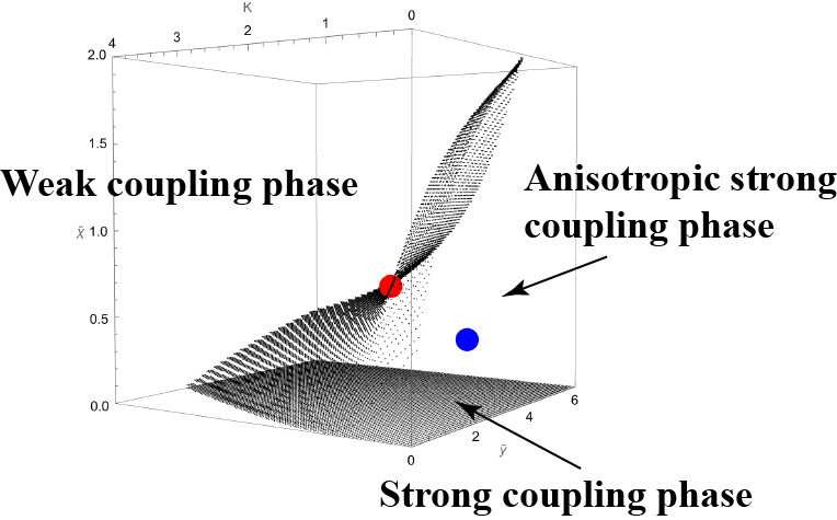
Figure S2: 3D RG phase diagram for $N=1$ case at subspace $\eta=0$. The blue point is the stable fixed point of the anisotropic strong coupling phase. The red point is the saddle-point fixed point that characterizes the weak-strong coupling phase transition. There are three phases: the weak coupling phase, the anisotropic strong coupling phase, and the strong coupling phase. The black dots form the boundary of these phases.

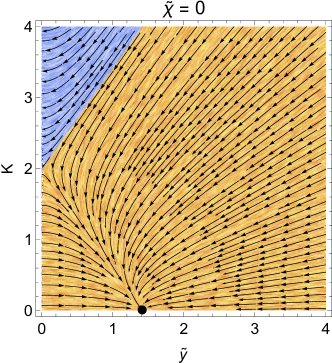
(a) subspace $\tilde{\chi}=0$

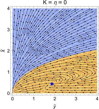
(b) subspace $K=\eta=0$

Figure S3: 2D cross-sections with RG flows of the 3D RG phase diagrams in Fig. S2. (a) 2D RG phase diagram at $\tilde{\chi}=0$. The black point is a fixed point of a strong coupling phase with $\tilde{\chi}_{1}=0$. (b) 2D RG phase diagram at $K=\eta=0$. The blue point is a stable fixed point for the strong coupling phase with $\tilde{\chi}_{1}\neq 0$. Blue and orange regions are weak and strong coupling phases, respectively, and arrows stand for RG flow in the infrared limit ($l\rightarrow\infty$).

III.5 $N\to 0$ case: Anderson transition and quasi-localization

The coupled RG equations in the zero replica limit are among six coupling constants, $y$, $\sigma_{x}$, $\sigma_{y}$, $c_{x}$, $c_{y}$ and $\chi_{y}$,

$$\frac{\mathrm{d}y}{\mathrm{d}l}=\left(2-\frac{1}{4}\frac{\sigma_{x}c_{y}+\sigma_{y}c_{x}+2\sigma_{x}\sigma_{y}}{2\sqrt{\sigma_{x}\sigma_{y}}}\right)y,$$ (S128)

$$\frac{\mathrm{d}\sigma_{\mu}}{\mathrm{d}l}=-\pi^{-1}y^{2}\sigma_{\mu}^{2}\lim_{N\to 0}B_{\mu},$$ (S129)

$$\frac{\mathrm{d}c_{\mu}}{\mathrm{d}l}=-\pi^{-1}y^{2}\sigma_{\mu}(\sigma_{\mu}+2c_{\mu})\lim_{N\to 0}B_{\mu},$$ (S130)

$$\frac{\mathrm{d}\chi_{y}}{\mathrm{d}l}=\chi_{y},$$ (S131)

with $\mu=x,y$. $\lim_{N\rightarrow 0}B_{\mu}$ is defined by

$$\lim_{N\rightarrow 0}B_{\mu}\equiv\frac{\mathrm{d}I_{\mu,N}}{\mathrm{d}N}\Big{|}_{N=0}+I_{\mu,0},$$ (S132)

with Eqs. (S113). Here we use,

$$\lim_{N\to 0}\frac{1}{N\Gamma(N)}=1,\quad\lim_{N\to 0}\frac{1}{N}\left[(\sigma_{\mu}+Nc_{\mu})^{2}-\frac{\sigma_{\mu}^{2}}{N+1}\right]=\sigma_{\mu}(\sigma_{\mu}+2c_{\mu}).$$ (S133)

$\lim_{N\to 0}B_{\mu}$ can be calculated from Eqs. (S113) with redefinitions of coupling constants,

$$\zeta \equiv\frac{\sigma_{x}}{\sigma_{y}},\quad\eta\equiv\frac{\sigma_{x}+c_{x}}{\sigma_{y}+c_{y}},\quad\lambda\equiv\frac{\zeta^{2}}{\eta}=\frac{\sigma^{2}_{x}}{\sigma^{2}_{y}}\frac{\sigma_{y}+c_{y}}{\sigma_{x}+c_{x}},\quad\tilde{\chi}\equiv\frac{\chi_{y}}{4\Lambda\sqrt{1+\zeta}}.$$ (S134)

In terms of these new constants, the limits are calculated as follows,

$$\tilde{B}_{x}\equiv\frac{1}{4\pi^{2}}\frac{\zeta}{\sigma_{x}+c_{x}}\frac{1}{\lambda}\lim_{N\to 0}B_{x}=\frac{2\zeta+(3+2\zeta)\tilde{\chi}^{2}+\frac{\zeta}{\lambda}(1-\zeta-(2+\zeta)\tilde{\chi}^{2})}{(1+\tilde{\chi}^{2})^{4}(1+\zeta)^{3}},$$ (S135)

$$\tilde{B}_{y}\equiv\frac{1}{4\pi^{2}}\frac{1}{\sigma_{x}+c_{x}}\frac{1}{\lambda}\lim_{N\to 0}B_{y}=\frac{\zeta-1+(13-4\zeta)\tilde{\chi}^{2}-5(2+\zeta)\tilde{\chi}^{4}+\frac{\zeta}{\lambda}(2-17\tilde{\chi}^{2}+5\tilde{\chi}^{4})}{(1+\tilde{\chi}^{2})^{5}(1+\zeta)^{3}}.$$ (S136)

Note that from Eqs. (S129,S130,S135,S136), $\lambda$ is invariant under the renormalization,

$$\frac{\mathrm{d}\ln\lambda}{\mathrm{d}l}=2\bigg{(}\frac{\mathrm{d}\ln\sigma_{x}}{\mathrm{d}l}-\frac{\mathrm{d}\ln\sigma_{y}}{\mathrm{d}l}\bigg{)}+\bigg{(}\frac{\mathrm{d}\ln(\sigma_{y}+c_{y})}{\mathrm{d}l}-\frac{\mathrm{d}\ln(\sigma_{x}+c_{x})}{\mathrm{d}l}\bigg{)}=0,$$ (S137)

because

$$2\frac{\mathrm{d}\ln\sigma_{\mu}}{\mathrm{d}l}=\frac{\mathrm{d}\ln(\sigma_{\mu}+c_{\mu})}{\mathrm{d}l}=-8\pi y^{2}(\sigma_{y}+c_{y})\frac{\sigma^{2}_{x}}{\sigma_{y}}\tilde{B}_{\mu},$$ (S138)

for $\mu=x,y$. Eq. (S138) also shows that $\sigma^{2}_{x}/(\sigma_{x}+c_{x})$ as well as $\sigma^{2}_{y}/(\sigma_{y}+c_{y})$ are invariant unon the renormalization. Thus, the RG equations among the six coupling constants can be reduced into closed-coupled differential equations among four coupling constants. The right hand side of Eq. (S138) suggests a usage of following normalized vortex fugacity as one of these four constants,

$$\tilde{y}\equiv y\sqrt{4\pi\lambda\sigma_{y}(\sigma_{x}+c_{x})}=y\sqrt{\frac{4\pi(\sigma_{y}+c_{y})\sigma^{2}_{x}}{\sigma_{y}}}.$$ (S139)

In fact, one can derive closed coupled RG equations among $\tilde{y}$, $\zeta$, $\tilde{\chi}$ and a stiffness parameter $K$,

$$K=\frac{1}{4}\frac{\sigma_{x}c_{y}+\sigma_{y}c_{x}+2\sigma_{x}\sigma_{y}}{2\sqrt{\sigma_{x}\sigma_{y}}}.$$ (S140)

The equations are given as follows,

$$\frac{\mathrm{d}\tilde{y}}{\mathrm{d}l}=\left[2-K-\frac{1}{2}\tilde{y}^{2}(2\tilde{B}_{x}+\tilde{B}_{y})\right]\tilde{y},$$ (S141)

$$\frac{\mathrm{d}K}{\mathrm{d}l}=-\tilde{y}^{2}\frac{\tilde{B}_{x}(3\zeta+\lambda)+\tilde{B}_{y}(\zeta+3\lambda)}{2(\zeta+\lambda)}K,$$ (S142)

$$\frac{\mathrm{d}\zeta}{\mathrm{d}l}=-\tilde{y}^{2}(\tilde{B}_{x}-\tilde{B}_{y})\zeta,$$ (S143)

$$\frac{\mathrm{d}\tilde{\chi}}{\mathrm{d}l}=\left[1-\frac{1}{2}\tilde{y}^{2}\frac{\tilde{B}_{x}-\tilde{B}_{y}}{1+\zeta}\right]\tilde{\chi}.$$ (S144)

Together with these closed equations, we have secondary equations for $\sigma_{x}$ and $\sigma_{y}$,

$$\frac{\mathrm{d}\ln\sigma_{\mu}}{\mathrm{d}l}=-\tilde{y}^{2}\tilde{B}_{\mu},$$ (S145)

for $\mu=x,y$. In summary, Eqs. (S141,S142,S143,S144) together with Eqs. (S135,S136) determine a RG phase diagram in a four-dimensional parameter space subtended by $\tilde{y}$, $K$, $\zeta$ and $\tilde{\chi}$. The RG phase diagram is characterized by stable and saddle-point fixed points, where stable fixed points of the differential equations characterize thermodynamic phases in the phase diagram and saddle-point fixed points characterize phase transitions among phases. In the following, we first enumerate all the stable fixed points in the four-dimensional parameter space. Using Eq. (S145), we further characterize the transport properties of these fixed points, and clarify fixed points of non-topological metal, topological metal, Anderson insulator, and quasi-localized phases, respectively. Note that the RG equations are derived perturbatively in the vortex fugacity $y$, so an application of the RG equations should be limited to weak and intermediate coupling regimes of $y$, e.g. $y<1/\sqrt{\sigma_{x}\sigma_{y}}$. For this reason, we do not discuss a structure of RG flows and fixed points in large $\tilde{y}$ region; $\tilde{y}\equiv y\sqrt{4\pi\lambda}\sqrt{\sigma_{y}(\sigma_{x}+c_{x})}$. The following argument applies to arbitrary finite (initial) $\lambda$.

III.6 fixed points at finite $\tilde{y}$

Fixed points at finite $\tilde{y}$ must satisfy the following equations simultaneously.

$$2-K-\frac{1}{2}\tilde{y}^{2}(2\tilde{B}_{x}+\tilde{B}_{y})=0,\quad\frac{\tilde{B}_{x}(3\zeta+\lambda)+\tilde{B}_{y}(\zeta+3\lambda)}{2(\zeta+\lambda)}K=0,\quad(\tilde{B}_{x}-\tilde{B}_{y})\zeta=0,\quad\left[1-\frac{1}{2}\tilde{y}^{2}\frac{\tilde{B}_{x}-\tilde{B}_{y}}{1+\zeta}\right]\tilde{\chi}=0.$$ (S146)

They are satisfied by the following points

• stable FP at $\tilde{y}=3.64...,\,K=0,\,\zeta=0,\,\tilde{\chi}=\pm 1.10...$ (quasi-localized phase).

• saddle-point FP at $\tilde{y}=3.56...,\,K=\frac{3}{4},\,\zeta=0,\,\tilde{\chi}=\pm 1.22...$ (quantum phase transition).

• saddle-point FP at $\tilde{y}=3.34...,\,K=0,\,\zeta=0,\,\tilde{\chi}=\pm 0.287...$.

• unstable FP at $\tilde{y}=\frac{2(1+\lambda)}{\sqrt{3}},\,K=0,\,\zeta=\lambda,\,\tilde{\chi}=0$.

• unstable FP at $\tilde{y}=2.98..,\,K=\frac{3}{4},\,\zeta=0,\,\tilde{\chi}=\pm 0.274...$.

As discussed below, the first one is a stable fixed point that characterizes the quasi-localized phase, and the second one is a saddle-point fixed point that characterizes a phase transition between quasi-localized and metal phases. Our extensive numerical investigations show no other fixed points with finite $\tilde{y}$. In the following, we will explain these fixed points in detail.

1. The stable FP at $(\tilde{y},K,\zeta,\tilde{\chi})=(3.64...,\,0,\,0,\,\pm 1.10..)$ characterizes quasi-localized phase at $\chi_{y}\neq 0$. This point is obtained by a condition of $K=\zeta=0$, and $2-\frac{1}{2}\tilde{y}^{2}(2\tilde{B}_{x}+\tilde{B}_{y})=0$ and $1-\frac{1}{2}\tilde{y}^{2}(\tilde{B}_{x}-\tilde{B}_{y})=0$, which leads to $\tilde{y}^{2}\tilde{B}_{x}=2$ and $\tilde{y}^{2}\tilde{B}_{y}=0$. $\tilde{y}^{2}\tilde{B}_{y}=0$ at $\zeta=0$ and $\tilde{y}\neq 0$ gives $-1+13\tilde{\chi}^{2}-10\tilde{\chi}^{4}=0$, while finite $\tilde{y}$ is determined by $\tilde{y}^{2}\tilde{B}_{x}=\frac{3\tilde{y}^{2}\tilde{\chi}^{2}}{(1+\tilde{\chi}^{2})^{4}}=2$. The RG equations can be linearized around the fixed point, revealing four RG eigenvalues around the fixed point as $-2.51..-i3.77..,-2.51..+i3.77..,-2,-1$. $``-2"$ is a scaling dimension for $\zeta$, and $``-1"$ is a scaling dimension for $K$. The linearized RG equations form an attractive flow with a swirl toward the fixed point in the $\tilde{y}$-$\tilde{\chi}$ plane. Around the fixed point, both $\zeta$ and $\sigma_{x}$ vanish with a same asymptotic form, $e^{-2l}$, because

   $$\frac{\mathrm{d}\ln\zeta}{\mathrm{d}l}=\frac{\mathrm{d}\ln\sigma_{x}}{\mathrm{d}l}=-\tilde{y}\tilde{B}_{x}=-2.$$ (S147)

   Thus, the conductivity $\sigma_{y}$ along the topological direction takes a finite value; $\sigma_{y}=\sigma_{x}/\zeta$. This stable fixed point characterizes a quasi-localized phase.

2. The saddle-point fixed point at $(\tilde{y},K,\zeta,\tilde{\chi})=(3.58...,\,3/4,\,0,\,\pm 1.22...)$ characterizes a phase transition between the quasi-localized phase and metal phase. The fixed point is obtained from a condition of $\zeta=0$, and $2-K-\frac{1}{2}\tilde{y}^{2}(2\tilde{B}_{x}+\tilde{B}_{y})=0$, $\tilde{y}^{2}(\tilde{B}_{x}+3\tilde{B}_{y})=0$, and $1-\frac{1}{2}\tilde{y}^{2}(\tilde{B}_{x}-\tilde{B}_{y})=0$, which leads to $\tilde{y}^{2}\tilde{B}_{x}=\frac{3}{2}$ and $\tilde{y}^{2}\tilde{B}_{y}=-\frac{1}{2}$, $K=3/4$. $\tilde{B}_{x}+3\tilde{B}_{y}=0$ at $\zeta=0$ gives $9\tilde{\chi}^{4}-14\tilde{\chi}^{2}+1=0$, while finite $\tilde{y}$ is determined by $\tilde{y}^{2}\tilde{B}_{x}=\frac{3}{2}$. The RG equations are linearized around the fixed point with RG eigenvalues; $-1.55..+3.41..i$, $-1.55..-3.41..i$, $-2$, $0.819..$. $``-2"$ is a scaling dimension for $\zeta$. Notably, the fixed point has one positive RG eigenvalue (“0.819..”), which stands for a scaling dimension of a relevant scaling variable. The relevant scaling variable is given by a linear superposition of $\delta\tilde{y}/\tilde{y}_{\rm FP}$, $\delta K/K_{\rm FP}$, and $\delta\tilde{\chi}/\tilde{\chi}_{\rm FP}$, while linear coefficients suggest that it is mainly $\delta K/K_{\rm FP}$. The critical exponent of the phase transition is given by $\nu=1/0.819..=1.22..$.

3. The saddle-point fixed point at $(\tilde{y},K,\zeta,\tilde{\chi})=(3.34..,\,0,\,0,\,\pm 0.287..)$ is from the same condition as the stable fixed point, $\tilde{B}_{y}=0$ and $\tilde{y}^{2}\tilde{B}_{x}=2$, while it is from the other solutions of $-1+13\tilde{\chi}^{2}-10\tilde{\chi}^{4}=0$. RG eigenvalues around the fixed point are $-5.73..,\,-2,\,-1,\,7.33..$, suggesting that it characterizes a phase transition with an extremely small critical exponent $1/7.33..=0.13..$. The exponent clearly breaks the Chayes inequality between the critical exponent $\nu$ and spatial dimension $d=2$ ($\nu d>2$) [47]. A numerical examination of the differential equations shows that the fixed point characterizes a phase transition between quasi-localized and a strong-coupling regime with infinitely large $\tilde{y}$. Since the perturbative RG equation can be applicable only for weak $\tilde{y}$ region, we regard the strong-coupling phase as well as this phase transition as unphysical.

4. The unstable fixed point at $(\tilde{y},K,\zeta,\tilde{\chi})=(2.98..,\,3/4,\,0,\,\pm 0.274..)$ is obtained from the same condition as the saddle-point fixed point at $K=3/4$, $\tilde{y}^{2}\tilde{B}_{x}=3/2$ and $\tilde{y}^{2}\tilde{B}_{y}=-1/2$, while it is from the other solutions of $9\tilde{\chi}^{4}-14\tilde{\chi}^{2}+1=0$. RG eigenvalues around the fixed point contain two positive values, $5.75..,\,-4.77..,\,-2,\,0.966..$. concluding that that it characterizes neither the criticality of a generic phase transition nor the thermodynamic phase.

5. The unstable fixed point at $(\tilde{y},K,\zeta,\tilde{\chi})=(\frac{2(1+\lambda)}{\sqrt{3}},\,0,\,\lambda,\,0)$ satisifies $\tilde{B}_{x}-\tilde{B}_{y}=0$, $\tilde{\chi}=K=0$, and $4-\tilde{y}^{2}(2\tilde{B}_{x}+\tilde{B}_{y})=0$. RG eigenvalues around this fixed point contain two positive values; $-4,\,-\frac{8}{3},\,\frac{4}{3},\,1$. $``1"$ is the scaling dimension of one of the two relevant scaling variables, $\tilde{\chi}$, and $``\frac{4}{3}"$ is the scaling dimension of the other relevant scaling variable, $\delta\zeta\equiv\zeta-\lambda$. Within a 2D space of $\tilde{\chi}=0$ (no topological term) and $\zeta=\lambda$, this fixed point is stable, and it characterizes the Anderson insulator phase [20]. However, the fixed point is unstable against an introduction of small $\delta\zeta$ as well as small $\chi$. The numerical examination shows that the small $\delta\zeta$ drives the RG flow into the strong coupling region with large $\tilde{y}$.

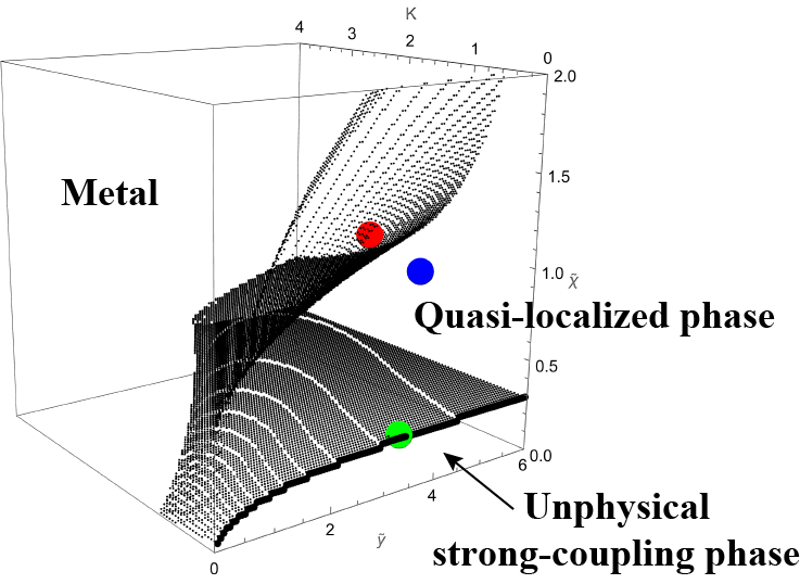
Figure S4: 3D RG phase diagram of $N\to 0$ case in the subspace $\zeta=0$ and $\lambda=1$. Blue and red points are stable fixed points for the quasi-localized phase, and saddle-point fixed points for a transition between quasi-localized and topological metal phases, respectively. The green dot is a saddle-point fixed point for a transition between quasi-localized and unphysical strong-coupling phase. The black dots form the boundary of different phases. The phase diagram is constructed by a numerical solution of the RG equations. For given initial values of $(\tilde{y}(l=0),(l=0),\tilde{\chi}(l=0))$, we solve the differential equations numerically and determine the infrared(IR)-limit values of $\tilde{y}(l)$, $K(l)$, and $\tilde{\chi}(l)$ for sufficiently large $l$. Parameter points in the metal phase reach the stable fixed region with $\tilde{y}^{2}\tilde{B}_{x}=0$, Parameter points in the quasi-localized phase reach the stable point with $\tilde{y}^{2}\tilde{B}_{x}\neq 0$ (blue point). Parameter points in the unphysical phase reach a strong-coupling region with divergent $\tilde{y}$.

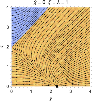
(a) subspace $\tilde{\chi}=0$, $\zeta=\lambda=1$

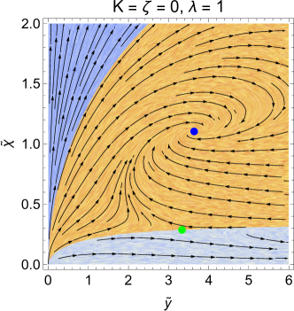
(b) subspace $K=\zeta=0$, $\lambda=1$

Figure S5: 2D cross-sections with RG flows of the 3D phase diagram in Fig. S4. (a) 2D RG phase diaram at $\tilde{\chi}=0$ and $\zeta=\lambda=1$. Blue and orange regions are nontopological metal and Anderson insulator phases respectively. The black point stands for a fixed point of the Anderson insulator phase. (b) 2D RG phase diagram at $K=\zeta=0$, and $\lambda=1$. Blue, orange, and light blue regions are topological metal, quasi-localized, and unphysical strong-coupling phases, respectively. The blue point is the stable fixed point of the quasi-localized phase. The green point is a saddle-point fixed point that characterizes a transition between the quasi-localized phase and the unphysical strong-coupling region. The arrow stands for the RG flow in the infrared limit ($l\rightarrow\infty$).

III.7 fixed points at $\tilde{y}=0$

Let us consider the RG equations around infinitesimally small $\tilde{y}$ or at $\tilde{y}=0$. When linearized with respect to small $\tilde{y}$, the coupled RG equations reduce to

$$\frac{\mathrm{d}\tilde{y}}{\mathrm{d}l}=(2-K)\tilde{y},\quad,\frac{\mathrm{d}\tilde{\chi}}{\mathrm{d}l}=\tilde{\chi},\quad,\frac{\mathrm{d}K}{\mathrm{d}l}=\frac{\mathrm{d}\zeta}{\mathrm{d}l}=0.$$ (S148)

The reduced RG equations have the following fixed regions,

• stable FP region at $(\tilde{y},K,\zeta,\tilde{\chi})=(0,K,\zeta,\infty)$ with $K>2$ (metal phase).

• unstable FP region at $(\tilde{y},K,\zeta,\tilde{\chi})=(0,K,\zeta,\infty)$ with $K<2$.

• unstable FP region at $(\tilde{y},K,\zeta,\tilde{\chi})=(0,K,\zeta,0)$.

The stable fixed region at $(\tilde{y},K,\zeta,\tilde{\chi})=(0,K,\zeta,\infty)$ with $K>2$ form a two-dimensional (2D) region subtended by $K$ and $\zeta$. It is stable against small $1/\tilde{\chi}$ as well as small $\tilde{y}$. At and around this fixed point, $\tilde{B}_{x}$ and $\tilde{B}_{y}$ vanish as $1/\tilde{\chi}^{6}$, and $\tilde{y}$ go to zero. Thus, the vanishing right hand side of Eq. (S145) suggests that both $\sigma_{x}$ and $\sigma_{y}$ reach finite values and the fixed region describes (topological) metal phase with $\chi_{y}\neq 0$. A fixed region at $(\tilde{y},K,\zeta,\tilde{\chi})=(0,K,\zeta,0)$ with $K<2$ characterizes a non-topological metal with $\chi_{y}=0$ [20], while it is always unstable against small $\tilde{\chi}$.

As discussed above, a general structure of the RG phase diagram in the $\tilde{y}$-$K$-$\zeta$-$\tilde{\chi}$ space has complications. Nonetheless, the phase diagram becomes simpler, when conductivity and Gade constant satisfy the following relatively generic condition,

$$\frac{\sigma_{x}}{\sigma_{y}}=\frac{\sigma_{x}+c_{x}}{\sigma_{y}+c_{y}},$$ (S149)

or equivalently $\zeta=\lambda$. This condition includes a case with isotropic conductivity and Gade constant; $\sigma_{x}=\sigma_{y}$ and $c_{x}=c_{y}$, When initial values of the constants satisfy this condition, the $K$-$\tilde{y}$-$\tilde{\chi}$ phase diagram at $\tilde{\chi}\neq 0$ comprises only of the quasi-localized and (topological) metal phases. As discussed above, these two phases are characterized by the stable fixed points at $(\tilde{y},K,\zeta,\tilde{\chi})=(3.64..,0,\,0,\,\pm 1.10...)$, and the stable 2D fixed region at $(\tilde{y},K,\zeta,\tilde{\chi})=(0,K,\,\zeta,\,\pm\infty)$, respectively, while the phase transition between these two phases are controlled by the saddle-point fixed point at $(\tilde{y},K,\zeta,\tilde{\chi})=(3.56..,0.75,\,0,\,\pm 1.22...)$. In Fig. S6, we show how $y$, $\sigma_{x}$, $\sigma_{y}$, $c_{x}$ and $c_{y}$ are renormalized along the RG equations for typical cases with this condition.

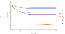
(a) A (topological) metal phase with $\chi_{y}\neq 0$

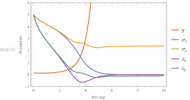
(b) Quasilocalized phase

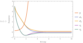
(c) Another parameter for quasi-localized phase

Figure S6: Numerical solutions of the RG equations. Initial values are chosen to be $\sigma_{x}=\sigma_{y}=c_{x}=c_{y}=5$, $\chi=0.1$ for all these three 3 figures, while (a) $y=0.1$, (b) $y=0.15$, and (c) $y=0.30$. The solution for (a) indicates that this parameter set is in the (topological) metal phase. The solution for (b) and (c) suggest that these parameter sets are in the quasi-localized phase.

IV Numerical simulation

IV.1 Tight-binding models

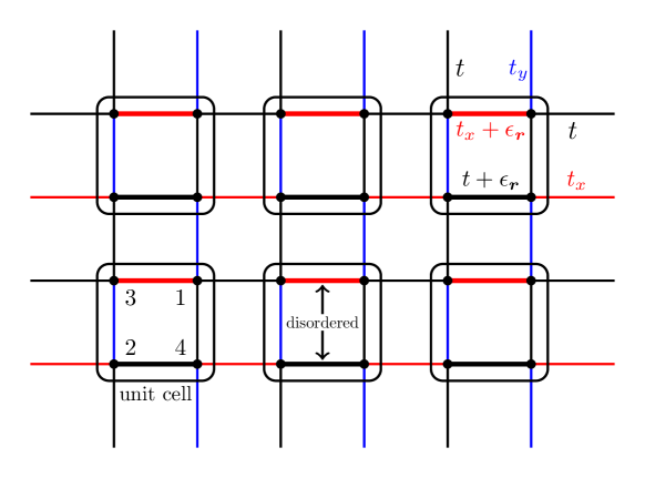
Figure S7: The two-dimensional square-lattice model with four inequivalent sublattice sites. Each unit cell (rectangle with rounded corners) contains four sublattice sites, labeled as 1, 2, 3, 4. Different hopping strengths are shown with different colors. Thinner links represent uniform hoppings (hopping without the disorder) such as $t$, $t_{y}$, and $t_{x}$, while thicker links represent the hoppings with complex-valued random variables such as $t_{x}+\epsilon_{\bm{r}}$, $t+\epsilon_{\bm{r}}$. Note that ${\bm{r}}$ stands for coordinates of the unit cell, and the complex-valued random variable is added only within the intra-unit-cell hopping term.

In the previous section, we show by the renormalization group analysis that the topological term ($\chi_{y}$) changes the nature of the localized phase proximate to the (critical) metal phase. Ref. [25] demonstrated numerically that a diffusive metal phase universally undergo a phase transition to the quasi-localized phase in three-dimensional (3D) chiral symmetric models with weak topology. In this section, we will demonstrate numerically that this is also the case with two-dimensional tight-binding chiral symmetric models with weak topology. We introduce a two-dimensional square-lattice model in chiral classes that has a weak topological index, i.e. one-dimensional topological winding number. The model in the clean limit was introduced previously [37]. A unit cell of the model has four inequivalent sublattice sites, 1, 2, 3, and 4. They are divided into two sublattice groups; (1,2) and (3,4). The model has no on-site terms and it comprises only hopping terms. The hopping terms are only between the two sublattice groups; no hopping within the same sublattice group.

$$H =\sum_{\bm{r}}\sum_{a,b=1,2,3,4}\ket{\bm{r},a}\bra{\bm{r},b}\begin{pmatrix}&&t_{x}+\epsilon_{\bm{r}}&t\\ &&t_{y}&t+\epsilon_{\bm{r}}\\ t_{x}+\epsilon_{\bm{r}}^{*}&t_{y}&&\\ t&t+\epsilon_{\bm{r}}^{*}&&\end{pmatrix}_{a,b}$$ (S150)

$$+\sum_{\bm{r},a,b}\ket{\bm{r},a}\bra{\bm{r}+\hat{\bm{x}},b}\begin{pmatrix}&&t&0\\ &&0&0\\ 0&0&&\\ 0&t_{x}&&\end{pmatrix}_{a,b}+\sum_{\bm{r},a,b}\ket{\bm{r},a}\bra{\bm{r}-\hat{\bm{x}},b}\begin{pmatrix}&&0&0\\ &&0&t_{x}\\ t&0&&\\ 0&0&&\end{pmatrix}_{a,b}$$

$$+\sum_{\bm{r},a,b}\ket{\bm{r},a}\bra{\bm{r}+\hat{\bm{y}},b}\begin{pmatrix}&&0&t_{y}\\ &&0&0\\ 0&t&&\\ 0&0&&\end{pmatrix}_{a,b}+\sum_{\bm{r},a,b}\ket{\bm{r},a}\bra{\bm{r}-\hat{\bm{y}},b}\begin{pmatrix}&&0&0\\ &&t&0\\ 0&0&&\\ t_{y}&0&&\end{pmatrix}_{a,b}.$$

Here ${\bm{r}}\equiv(n_{x},n_{y})$, ${\bm{r}}\pm\hat{\bm{x}}\equiv(n_{x}\pm 1,n_{y})$, ${\bm{r}}\pm\hat{\bm{y}}\equiv(n_{x},n_{y}\pm 1)$ specify the unit cell of the model; unit cells also form a square lattice (see Fig. S7). “$a$” and “$b$” specify sublattice site within the unit cell, $a,b=1,2,3,4$. The first term in Eq. (S150) stands for intra-unit-cell hopping terms, while the others are inter-unit-cell hopping terms. A complex-valued random hopping $\epsilon_{\bm{r}}$ is introduced in the intra-unit-cell hopping term. Real and imaginary parts of $\epsilon_{\bm{r}}$ are uniformly distributed in a range of $[-W/2,W/2]$; $W$ stands for the disorder strength of the model. Other hopping terms take finite definite real values.

The model has the chiral symmetry, $\sigma_{3}H\sigma_{3}=-H$, where $\sigma_{3}$ takes +1 for one of the two sublattice groups, e.g. (1,2), and takes $-1$ for the other sublattice group, (3,4). Since $H=H^{*}$, the model in the clean limit ($W=0$) belongs to the chiral orthogonal class (class BDI). In the presence of $\epsilon_{\bm{r}}$, the model breaks the time-reversal symmetry, belonging to the chiral unitary class (class AIII).

Due to the chiral symmetry, $H$ takes a block-off-diagonal form, $H=\sigma_{+}\otimes h+\sigma_{-}\otimes h^{\dagger}$ where the off-diagonal block $h$ is a non-Hermitian matrix,

$$h =\sum_{\bm{r},a,b}\ket{\bm{r},a}\bra{\bm{r},b}\begin{pmatrix}t_{x}+\epsilon_{\bm{r}}&t\\ t_{y}&t+\epsilon_{\bm{r}}\end{pmatrix}_{a,b}$$

$$+\sum_{\bm{r},a,b}\ket{\bm{r},a}\bra{\bm{r}+\hat{\bm{x}},b}\begin{pmatrix}t&0\\ 0&0\end{pmatrix}_{a,b}+\sum_{\bm{r},a,b}\ket{\bm{r},a}\bra{\bm{r}-\hat{\bm{x}},b}\begin{pmatrix}0&0\\ 0&t_{x}\end{pmatrix}_{a,b}$$

$$+\sum_{\bm{r},a,b}\ket{\bm{r},a}\bra{\bm{r}+\hat{\bm{y}},b}\begin{pmatrix}0&t_{y}\\ 0&0\end{pmatrix}_{a,b}+\sum_{\bm{r},a,b}\ket{\bm{r},a}\bra{\bm{r}-\hat{\bm{y}},b}\begin{pmatrix}0&0\\ t&0\end{pmatrix}_{a,b}.$$ (S151)

The weak topological index of $H$ is defined by $h$ with an attachment of uniform magnetic fluxes. Let us attach the magnetic flux $\phi_{\mu}$ into the hopping terms along $\mu$ of $h$; $h\rightarrow h(\phi_{\mu})$. In $h(\phi_{\mu})$, a particle that travels around the system with the periodic boundary condition along $\mu$ direction acquires a phase $e^{i\phi_{\mu}}$ for every round. In terms of such $h(\phi_{\mu})$, the winding number along $\mu$ is defined by [38, 13, 39]

$$\nu_{\mu}\equiv\frac{i}{L}\int^{\pi}_{-\pi}\frac{d\phi_{\mu}}{2\pi}\partial_{\phi_{\mu}}{\rm Tr}\big{[}\log[h(\phi_{\mu})]\big{]}=\frac{i}{L}\int^{\pi}_{-\pi}\frac{d\phi_{\mu}}{2\pi}\partial_{\phi_{\mu}}\log\big{[}\det[h(\phi_{\mu})]\big{]}.$$ (S152)

Here $L$ is a linear dimension of the system size along the transverse direction to $\mu$. In the clean limit ($W=0$), $(\nu_{x},\nu_{y})=(-1,0)$ for $|t_{x}|>|t_{y}|$, and $(\nu_{x},\nu_{y})=(0,1)$ for $|t_{x}|<|t_{y}|$. In some regions of $t_{x}=t_{y}$ and $|t_{x}+t_{y}|<2t$, the model also has finite winding numbers, but the numbers are not quantized to integers. Note also that $\nu_{\mu}=0$ whenever $t_{\mu}=\pm t$ (see Fig. S8 for details).

$\nu_{\mu}$ is zero at $t_{\mu}=\pm t$ for disordered systems, when $\nu_{\mu}$ is averaged over different disorder realizations. This is because an ensemble of $h$ with different disorder realizations is symmetric under certain symmetry operations at these special points [25]. For example, consider $t_{x}=t$, where an ensemble of $h$ is symmetric under a transposition followed by $\tau_{1}$ and a mirror. $\tau_{1}$ exchanges the sublattice index of $h$ and the mirror exchange a pair of two sites, $r=(n_{x},n_{y})$ and ${\bm{r}}^{\prime}=(n_{x},-n_{y})$;

$${\cal U}_{y,{(n_{x},n_{y}|n^{\prime}_{x},n^{\prime}_{y})}}=\delta_{n_{x},n^{\prime}_{x}}\delta_{n_{y},-n^{\prime}_{y}}.$$ (S153)

The transposition of $h$ followed by $\tau_{1}$ and ${\cal U}_{y}$ is given by

$${\cal U}_{y}\!\ \tau_{1}h^{T}\tau_{1}\!\ {\cal U}_{y} =\sum_{\bm{r},a,b}\ket{\bm{r},a}\bra{\bm{r},b}\begin{pmatrix}t+\epsilon_{(n_{x},-n_{y})}&t\\ t_{y}&t_{x}+\epsilon_{(n_{x},-n_{y})}\end{pmatrix}_{a,b}$$

$$+\sum_{\bm{r},a,b}\ket{\bm{r},a}\bra{\bm{r}+\hat{\bm{x}},b}\begin{pmatrix}t_{x}&0\\ 0&0\end{pmatrix}_{a,b}+\sum_{\bm{r},a,b}\ket{\bm{r},a}\bra{\bm{r}-\hat{\bm{x}},b}\begin{pmatrix}0&0\\ 0&t\end{pmatrix}_{a,b}$$

$$+\sum_{\bm{r},a,b}\ket{\bm{r},a}\bra{\bm{r}+\hat{\bm{y}},b}\begin{pmatrix}0&t_{y}\\ 0&0\end{pmatrix}_{a,b}+\sum_{\bm{r},a,b}\ket{\bm{r},a}\bra{\bm{r}-\hat{\bm{y}},b}\begin{pmatrix}0&0\\ t&0\end{pmatrix}_{a,b}.$$ (S154)

A statistical distribution of $\epsilon_{(n_{x},n_{y})}$ is same as that of $\epsilon_{(n_{x},-n_{y})}$. Thus, when $t_{x}=t$, an ensemble of the right hand side of Eq. (S154) over different disorder realizations is same as that of Eq. (S151);

$$\Big{\{}\!\ {\cal U}_{y}\!\ \tau_{1}h^{T}\tau_{1}\!\ {\cal U}_{y}\!\ \Big{|}\!\ \epsilon_{\bm{r}}\in\big{[}-\frac{W}{2},\frac{W}{2}\big{]}\!\ \Big{\}}=\Big{\{}\!\ h\!\ \Big{|}\!\ \epsilon_{\bm{r}}\in\big{[}-\frac{W}{2},\frac{W}{2}\big{]}\!\ \Big{\}},\quad\quad@\!\ t=t_{x}.$$ (S155)

The relation is generalized into cases with the magnetic flux along $x$ and/or $y$,

$$\Big{\{}\!\ {\cal U}_{y}\!\ \tau_{1}h^{T}(\phi_{x},\phi_{y})\tau_{1}\!\ {\cal U}_{y}\!\ \Big{|}\!\ \epsilon_{\bm{r}}\in\big{[}-\frac{W}{2},\frac{W}{2}\big{]}\!\ \Big{\}}=\Big{\{}\!\ h(-\phi_{x},\phi_{y})\!\ \Big{|}\!\ \epsilon_{\bm{r}}\in\big{[}-\frac{W}{2},\frac{W}{2}\big{]}\!\ \Big{\}},\quad\quad@\!\ t=t_{x}.$$ (S156)

Here both $\phi_{x}$ and $\phi_{y}$ change their signs under the transposition, while only $\phi_{y}$ changes its sign under the mirror ${\cal U}_{y}$. Note that $\nu_{\mu}$ stands for a phase winding of the U(1) phase of $\det h(\phi_{\mu})$ from $\phi_{\mu}=-\pi$ to $\phi_{\mu}=\pi$. Thus, the statistical symmetry of the ensemble requires that the average of $\nu_{x}$ must be zero at $t_{x}=t$. Similarly, an ensemble of $h$ at $t_{y}=t$ is statistically symmetric under the transposition followed by a spatial mirror ${\cal U}_{x}$,

$$\Big{\{}\!\ {\cal U}_{x}\!\ h^{T}(\phi_{x},\phi_{y})\!\ {\cal U}_{x}\!\ \Big{|}\!\ \epsilon_{\bm{r}}\in\big{[}-\frac{W}{2},\frac{W}{2}\big{]}\!\ \Big{\}}=\Big{\{}\!\ h(\phi_{x},-\phi_{y})\!\ \Big{|}\!\ \epsilon_{\bm{r}}\in\big{[}-\frac{W}{2},\frac{W}{2}\big{]}\!\ \Big{\}},\quad\quad@\!\ t=t_{y},$$ (S157)

with

$${\cal U}_{x,{(n_{x},n_{y}|n^{\prime}_{x},n^{\prime}_{y})}}\equiv\delta_{n_{x},-n^{\prime}_{x}}\delta_{n_{y},n^{\prime}_{y}}.$$ (S158)

The symmetry leads to $\nu_{y}=0$ at $t_{y}=t$.

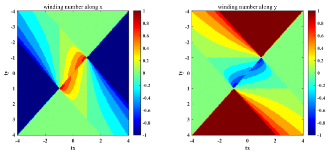
Figure S8: Distribution of one-dimensional winding numbers along $x$- and $y$-directions in a parameter space of $t_{x}$ and $t_{y}$ (the unit is $t$). Color represents the value of the winding numbers.

In the following numerical simulation, we choose $t_{x}=t$ and $t_{y}\neq t$ with $\nu_{y}\neq 0$ and $\nu_{x}=0$. This corresponds to the topological case with $\vec{\chi}=(0,\chi_{y})$ in the previous section. We also study $t_{x}=t_{y}=t$ with $\nu_{x}=\nu_{y}=0$. This point corresponds to the non-topological case ($\vec{\chi}=0$) in the chiral unitary class.

IV.2 Transfer matrix

The zero energy state of $H$ respects the chiral symmetry. An exponential localization length of the zero-energy state can be calculated via the transfer matrix method. To calculate the localization length $\xi_{x}$ along $x$, we consider a quasi-1D geometry with $L_{x}\times L_{y}$ unit cells and $L_{x}\gg L_{y}$; $L_{x}$ and $L_{y}$ are linear dimensions of the system size along $x$ and $y$ respectively. The quasi-1D system is regarded as $L_{x}$ slices of subsystems, and each subsystem has $L_{y}$ unit cells along $y$. The zero-energy state $\ket{\Psi}$ is partitioned into the $L_{x}$ slices, $\ket{\Psi}=[\cdots,\ket{\Psi}_{x-1},\ket{\Psi}_{x},\ket{\Psi}_{x+1},\cdots]$, where $\ket{\Psi}_{x}$ is a part of $\ket{\Psi}$ at the $x$-th slice. The Schrodinger equation for $\ket{\Psi}$ can be rewritten into a recursive relation between $\ket{\Psi}_{x+1}$ and $\ket{\Psi}_{x}$ (or between $[\ket{\Psi}_{x+1},\ket{\Psi}_{x}]$ and $[\ket{\Psi}_{x},\ket{\Psi}_{x-1}]$ in other models); $\ket{\Psi}_{x+1}=T_{x\rightarrow x+1}\ket{\Psi}_{x}$. Here a matrix $T_{x\to x+1}$ is called a transfer matrix. Since the unit cell has four inequivalent sublattices, the transfer matrix thus introduced is $4L_{y}$ by $4L_{y}$. We calculate all singular values of a product of transfer matrices along $x$,

$$\Omega\equiv\lim_{L_{x}\to\infty}\frac{1}{2L_{x}}\ln(T_{1\to L_{x}}^{\dagger}T_{1\to L_{x}}),\quad T_{1\to L_{x}}\equiv\prod_{n=1}^{L_{x}-1}T_{n\to n+1}.$$ (S159)

The eigenvalues of $\Omega$ are called Lyapunov exponents (LEs); $\{\gamma_{1},\gamma_{2},\cdots,\gamma_{4L_{y}}\}$ with $\gamma_{1}<\gamma_{2}<\gamma_{3}<\cdots<\gamma_{4L_{y}-1}<\gamma_{4L_{y}}$. The Hermicity of $H$ ensures the eigenvalues are symmetric with respect to zero, $\gamma_{j}=-\gamma_{4L_{y}-(j-1)}$. Since the product relates the $\ket{\Psi}_{L_{x}}$ and $\ket{\Psi}_{1}$, the smallest nonnegative LE $\gamma\equiv\gamma_{NL+1}$ is related to the exponential localization length $\xi_{x}$ of the zero-energy eigenstate along $x$ direction; $\xi_{x}=\gamma^{-1}$.

The zero-energy state of $H$ $\ket{\Psi}$ is given by zero-energy eigenstate $\ket{\Phi}$ of its non-Hermitian off-diagonal-block matrices $h$, $\ket{\Psi}=[0,\ket{\Phi}]^{T}$ [26]. Also it is given by zero-energy eigenstate $\ket{\Phi}^{\prime}$ of the other off-diagonal-block $h^{\dagger}$, $\ket{\Psi}=[\ket{\Phi}^{\prime},0]^{T}$. Consequently, the transfer matrix of $H$ can be block diagonalized into transfer matrices of $h$ and $h^{\dagger}$, where the LEs of the zero-energy state of $H$ is the union of the LEs of the zero-energy states of $h$ and $h^{\dagger}$. The transfer matrix of $h$ is obtained from the Schrodinger equation for $\ket{\Phi}$;

$$\left(\begin{array}[]{cc}t_{x}+\epsilon_{x,y}&t\\ t_{y}&t+\epsilon_{x,y}\\ \end{array}\right)\Phi_{x,y}+\left(\begin{array}[]{cc}0&0\\ t&0\\ \end{array}\right)\Phi_{x,y-1}+\left(\begin{array}[]{cc}0&t_{y}\\ 0&0\\ \end{array}\right)\Phi_{x,y+1}+\left(\begin{array}[]{cc}0&0\\ 0&t_{x}\\ \end{array}\right)\Phi_{x-1,y}+\left(\begin{array}[]{cc}t&0\\ 0&0\\ \end{array}\right)\Phi_{x+1,y}=0.$$ (S170)

Here $\ket{\Phi}$ is sliced into $L_{x}$ pieces; $\ket{\Phi}=[\cdots,\ket{\Phi}_{x-1},\ket{\Phi}_{x},\ket{\Phi}_{x+1},\cdots]$, and $\Phi_{x,y}$ is the $y$-th component of $\ket{\Phi}_{x}$; $\ket{\Phi}_{x}=[\cdots,\Phi_{x,y-1},\Phi_{x,y},\Phi_{x,y+1},\cdots]$. $\Phi_{x,y}$ has two components, $\Phi_{x,y}\equiv[\psi_{x,y},\phi_{x,y}]^{T}$. By solving the Schrodinger equation for $\psi_{x+1,y}$ and $\phi_{x+1,y}$ in terms of $\psi_{x,\cdots}$ and $\phi_{x,\cdots}$, one obtain

$$\psi_{x+1,y} =-\frac{t_{x}+\epsilon_{x,y}}{t}\psi_{x,y}-\phi_{x,y}-\frac{t_{y}}{t}\phi_{x,y+1}$$

$$\phi_{x+1,y} =\frac{t_{y}(t_{x}+\epsilon_{x,y})}{t(t+\epsilon_{x+1,y})}\psi_{x,y}+\frac{2t_{y}-t_{x}}{t+\epsilon_{x+1,y}}\phi_{x,y}+\frac{t_{x}+\epsilon_{x,y-1}}{t+\epsilon_{x+1,y}}\psi_{x,y-1}+\frac{t}{t+\epsilon_{x+1,y}}\phi_{x,y-1}+\frac{t^{2}_{y}}{t(t+\epsilon_{x+1,y})}\phi_{x,y+1}.$$

The equation relates $\ket{\Phi}_{x+1}$ with $\ket{\Phi}_{x}$ by a transfer matrix $\hat{M}_{x\rightarrow x+1}$;

$$\ket{\Phi}_{x+1}=M_{x\to x+1}\ket{\Phi}_{x}$$ (S171)

with

$$[M_{x\to x+1}]_{(y,a|y^{\prime},b)}$$

$$\ \ =\left(\begin{array}[]{cc}-\frac{t_{x}+\epsilon_{x,y}}{t}&-1\\ \frac{t_{y}(t_{x}+\epsilon_{x,y})}{t(t+\epsilon_{x+1,y})}&\frac{2t_{y}-t_{x}}{t+\epsilon_{x+1,y}}\\ \end{array}\right)_{a,b}\delta_{y,y^{\prime}}+\left(\begin{array}[]{cc}0&-\frac{t_{y}}{t}\\ 0&\frac{t^{2}_{y}}{t(t+\epsilon_{x+1,y})}\end{array}\right)_{a,b}\delta_{y+1,y^{\prime}}+\left(\begin{array}[]{cc}0&0\\ \frac{t_{x}+\epsilon_{x,y-1}}{t+\epsilon_{x+1,y}}&\frac{t}{t+\epsilon_{x+1,y}}\\ \end{array}\right)_{a,b}\delta_{y-1,y^{\prime}}.$$ (S178)

Similarly, for $h^{\dagger}$, the zero-energy state $\ket{\Phi}^{\prime}$ is sliced into the $L_{x}$ pieces, $\ket{\Phi}^{\prime}=[\cdots,\ket{\Phi}^{\prime}_{x+1},\ket{\Phi}^{\prime}_{x},\ket{\Phi}^{\prime}_{x-1},\cdots]$, and $\ket{\Phi}^{\prime}_{x+1}$ and $\ket{\Phi}^{\prime}_{x}$ are recursively related by the transfer matrix of $h^{\dagger}$,

$$\ket{\Phi}^{\prime}_{x+1}=M^{\prime}_{x\rightarrow x+1}\ket{\Phi}^{\prime}_{x}.$$ (S179)

The Schrodinger equation for $\ket{\Phi}^{\prime}$ is

$$\left(\begin{array}[]{cc}t_{x}+\epsilon_{x,y}^{*}&t_{y}\\ t&t+\epsilon_{x,y}^{*}\\ \end{array}\right)\Phi_{x,y}^{\prime}+\left(\begin{array}[]{cc}0&t\\ 0&0\\ \end{array}\right)\Phi_{x,y+1}^{\prime}+\left(\begin{array}[]{cc}0&0\\ t_{y}&0\\ \end{array}\right)\Phi_{x,y-1}^{\prime}+\left(\begin{array}[]{cc}0&0\\ 0&t_{x}\\ \end{array}\right)\Phi_{x+1,y}^{\prime}+\left(\begin{array}[]{cc}t&0\\ 0&0\\ \end{array}\right)\Phi_{x-1,y}^{\prime}=0,$$ (S190)

which lead to

$$[M^{\prime}_{x\rightarrow x+1}]_{(y,a|y^{\prime},b)}$$ (S191)

$$=\begin{pmatrix}\frac{t(2t_{y}-t_{x})}{t_{x}(t_{x}+\epsilon_{x+1,y}^{*})}&\frac{t_{y}(t+\epsilon_{x,y}^{*})}{t_{x}(t_{x}+\epsilon_{x+1,y}^{*})}\\ -\frac{t}{t_{x}}&-\frac{t+\epsilon_{x,y}^{*}}{t_{x}}\end{pmatrix}_{a,b}\delta_{y,y^{\prime}}+\begin{pmatrix}\frac{t^{2}}{t_{x}(t_{x}+\epsilon_{x+1,y}^{*})}&\frac{t(t+\epsilon_{x,y+1}^{*})}{t_{x}(t_{x}+\epsilon_{x+1,y}^{*})}\\ 0&0\end{pmatrix}_{a,b}\delta_{y+1,y^{\prime}}+\begin{pmatrix}\frac{t_{y}^{2}}{t_{x}(t_{x}+\epsilon_{x+1,y}^{*})}&0\\ -\frac{t_{y}}{t_{x}}&0\end{pmatrix}_{a,b}\delta_{y-1,y^{\prime}},$$ (S192)

In terms of $M_{x\rightarrow x+1}$ and $M^{\prime}_{x\rightarrow x+1}$, the transfer matrix of $H$ is given by the block-diagonal form,

$$T_{x\rightarrow x+1}=\left(\begin{array}[]{cc}M^{\prime}_{x\rightarrow x+1}&0\\ 0&M_{x\rightarrow x+1}\\ \end{array}\right).$$ (S195)

Due to the block-diagonal form, the LEs of $H$ are given by a union of the LEs of $h$ and $h^{\dagger}$. We confirmed numerically that the LEs of $M^{\prime}$ are exactly the opposite numbers of the LEs of $M$. We thus expect that $M^{\prime}_{x\rightarrow x+1}$ and $M^{-1}_{x\rightarrow x+1}$ are related to each other by a non-singular similarity transformation.

Likewise, To calculate the localization length $\xi_{y}$ along $y$, we consider a quasi-1D geometry with $L_{x}\times L_{y}$ unit cells and $L_{y}\gg L_{x}$. We slice the zero-energy state $\ket{\Phi}$ into $L_{y}$ pieces; $\ket{\Phi}=[\cdots,\ket{\Phi}_{y-1},\ket{\Phi}_{y},\ket{\Phi}_{y+1},\cdots]$, and relate $\ket{\Phi}_{y-1}$ with $\ket{\Phi}_{y}$ by a transfer matrix $\hat{M}_{y\rightarrow y-1}$,

$$\ket{\Phi}_{y-1}=M_{y\to y-1}\ket{\Phi}_{y}$$ (S196)

with

$$[M_{y\to y-1}]_{(x,a|x^{\prime},b)}$$

$$\ \ =\left(\begin{array}[]{cc}-\frac{t_{y}}{t}&-\frac{t+\epsilon_{x,y}}{t}\\ \frac{t_{y}(t_{x}+\epsilon_{x,y-1})}{t^{2}}&\frac{(t_{x}+\epsilon_{x,y-1})(t+\epsilon_{x,y})+(t_{x}-t_{y})t}{t^{2}}\\ \end{array}\right)_{a,b}\delta_{x,x^{\prime}}+\left(\begin{array}[]{cc}0&0\\ \frac{t_{y}}{t}&\frac{t+\epsilon_{x+1,y}}{t}\end{array}\right)_{a,b}\delta_{x+1,x^{\prime}}+\left(\begin{array}[]{cc}0&-\frac{t_{x}}{t}\\ 0&\frac{t_{x}(t_{x}+\epsilon_{x,y-1})}{t^{2}}\\ \end{array}\right)_{a,b}\delta_{x-1,x^{\prime}}.$$ (S203)

In terms of these transfer matrices, we calculate the LEs of the zero-energy state of $h$ along $x$ and $y$ from the eigenvalues of the following two matrices,

$$\Omega_{h,x} \equiv\lim_{L_{x}\rightarrow\infty}\frac{1}{2L_{x}}\ln\Big{(}M^{\dagger}_{1\to L_{x}}M_{1\to L_{x}}\Big{)},\quad M_{1\to L_{x}}\equiv\prod^{L_{x}-1}_{n=1}M_{n\to n+1},$$

$$\Omega_{h,y} \equiv\lim_{L_{y}\rightarrow\infty}\frac{1}{2L_{y}}\ln\Big{(}M^{\dagger}_{L_{y}\to 1}M_{L_{y}\to 1}\Big{)},\quad M_{L_{y}\to 1}\equiv\prod^{1}_{n=L_{y}-1}M_{n+1\to n},$$

For $t_{x}=t$ and $t_{y}\neq t$, an ensemble of $h$ has the transpositional symmetry accompanied by the mirror $U_{y}$, Eq. (S155). Since the transposition changes signs of LEs along $x$ and the mirror does not, a set of the LEs of $h$ along $x$ become statistically symmetric with respect to zero; $\gamma_{x,1}<\gamma_{x,2}<\cdots<\gamma_{x,2L_{y}-1},\gamma_{x,2L_{y}}$ with $\gamma_{x,j}=\gamma_{x,2L_{y}-(j-1)}$. Meanwhile, since both the transposition and the mirror change the sign along $y$, a set of the LEs of $h$ along $y$ are not necessarily symmetric with respect to zero. More generally, a number $N_{y,+}$ of positive LEs along $y$ can be different from a number $N_{y,-}$ of negative LEs along $y$, and their difference is related to the topological winding number along $y$ as $\nu_{y}=\frac{1}{2L_{x}}(N_{y,+}-N_{y,-})$ [25] (see also Fig. S9(c)).

(a)

(b)

(c)

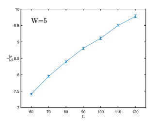
(d)

(e)

Figure S9: (a) Ditributions of the LEs of the zero-energy state of $h$ as a function of the disorder strength $W$. (left) The LEs of $h$ along the $x$-direction. The distributions of the LEs along $x$ are symmetric with respect to zero. (right) The LEs of $h$ along the $y$-direction. The LEs along $y$ cross zero when $2<W<5.12$. In the thermodynamic limit ($L_{x}\rightarrow\infty$), these LEs form a continuous band, and the band covers the zero when $2<W<5.12$. (b) The one-dimensional topological winding number $\nu_{y}$ along $y$ as a function of the disorder strength $W$. The blue curve plots $\nu_{y}=\frac{1}{2L_{x}}(N_{y,+}-N_{y,-})$, where $N_{y,\pm}$ are calculated from the numbers of positive/negative LEs of $h$ along $y$, respectively. The orange dots are $\nu_{y}$ calculated by a real space formula of the winding number [48, 38]. (c) Inverse normalized localization lengths $\frac{L_{\perp}}{\xi_{\mu}}$ along $x$ ($\mu=x,L_{\perp}=L_{y}$; red) and along $y$ ($\mu=y,L_{\perp}=L_{x}$; blue) as a function of the disorder strength $W$ for different system sizes $L_{\perp}=60,70,80,90,100,110,120$. $(t_{x},t_{y})=t(1,1.5)$. For both $\mu=x$ and $\mu=y$ and for larger $W$, $\frac{L_{\perp}}{\xi_{\mu}}$ increases when the system size $L_{\perp}$ increases. $W^{(c)}_{y}$ is a critical point below which $\xi_{y}$ being zero in the thermodynamic limit $(L_{x}\rightarrow\infty)$. $W^{(c)}_{y}$ is determined by a finite size scaling [25]. For $W$ close to but below $W_{y}^{(c)}=5.1204$, $\frac{L_{y}}{\xi_{x}}$ becomes larger for larger $L_{y}$, indicating a finite exponential localization length along $x$ for a certain regime below $W<W^{(c)}_{y}$. (d) Inverse normalized localization length along $x$-direction $\frac{L_{y}}{\xi_{x}}$ as a function of $L_{y}$ at $W=5<W^{(c)}_{y}$. (e) (upper) Schematic phase diagram around $W=5$ for $(t_{x}.t_{y})=t(1,1.5)$. (lower) schematic phase diagram around $W=2.5$ for $(t_{x},t_{y})=t(1,1)$

Fig. S9 shows numerical results of the transfer matrix calculation at $t_{x}=t$ and $t_{y}=1.5t$, where the model is in the chiral unitary class with $\nu_{x}=0$ and $\nu_{y}\neq 0$. The LEs of the zero-energy state of $h$ along $x$ and $y$ are calculated with the quasi-1D geometry, $L_{\perp}\times L_{\parallel}$, where $L_{\perp}=60\sim 120$ and $L_{\parallel}=10^{6}$. Fig. S9(a) shows a distribution of all the LEs along $x$ (right) and $y$ (left). The LEs along $x$ are distributed symmetrically around zero, being consistent with the statistical symmetry of $h$ at $t_{x}=t$ and $t_{y}\neq t$. The LEs along $y$ are distributed asymmetrically around zero. Moreover, all the LEs along $y$ are positive near the clean limit, $N_{y,+}=2L_{x}$ and $N_{y,-}=0$, so that $\nu_{y}=(N_{y,+}-N_{y,-})/(2L_{x})=1$. Upon increasing the disorder strength $W$, some of the LEs along $y$ decrease and become negative for $W\gtrsim 2$. For $W>W^{(c)}_{y}$, a lower half of the LEs along $y$ become negative, while the upper half of the LEs along $y$ are positive; $N_{y,+}=L_{x}$, $N_{y,-}=L_{x}$ and $\nu_{y}=(N_{y,+}-N_{y,-})/(2L_{x})=0$.

The lower half of the LEs along $y$ form a continuous band in the thermodynamic limit $(L_{x}\rightarrow\infty)$ [42], and the band covers the zero for $W^{(c)}_{y}>W\gtrsim 2$. Thereby, $0<N_{y.-}<L_{x}<N_{y,+}$ and $0<\nu_{y}<1$ (Fig. S9(b)). This means that for $W^{(c)}_{y}>W\gtrsim 2$, the exponential localization length along $y$ is always divergent in the thermodynamic limit (Fig. S9(c)). The value of $W^{(c)}_{y}$ is determined by a fitting of the largest LE in the lower half of the LEs of $h$ along $y$, $W^{(c)}_{y}\approx 5.1204\pm 0.002$.

Importantly, the localization length $\xi_{x}$ along $x$ undergoes a metal-insulator transition near $W^{(c)}_{y}$. In the insulator phase, $\xi_{x}/L_{y}\equiv 1/(\gamma_{x}L_{y})$ decreases for increasing $L_{y}$ (see Fig. S9(d)). In the (critical) metal phase, $\xi_{x}/L_{y}$ stays invariant for increasing $L_{y}$. We determine a critical disorder strength $W^{(c)}_{x}$ for the change of $\xi_{x}/L_{y}$ by a fitting of $\mathrm{d}(\gamma_{x}L_{y})/\mathrm{d}L_{y}$ (see Fig. 3(b) in the main text). $W^{(c)}_{x}$ thus determined turns out to be clearly smaller than $W^{(c)}_{y}$, $W^{(c)}_{x}=4.979\pm 0.016$. A discrepancy between $W^{(c)}_{x}$ and $W^{(c)}_{y}$ is about $3\%$ of the critical values, and it is far larger than the error bars of the fittings. This indicates the emergence of the quasi-localized phase between metal and Anderson localized phases.

In summary, upon increasing $W$, the model undergoes a phase transition from topological metal phase ($\nu_{y}\neq 0$, $W<W^{(c)}_{x}$) to quasi-localized phase ($\nu_{y}\neq 0$, $W^{(c)}_{x}<W<W^{(c)}_{y}$), and then undergoes another phase transition from quasi-localized phase to Anderson localized phase ($\nu_{y}=0$, $W^{(c)}_{y}<W$) (upper panel of Fig. S9(e)). In the quasi-localized phase with $\nu_{y}\neq 0$, the exponential localization length along $y$ is divergent, while the localization length along $x$ is finite.

Fig. S10 shows numerical results of the transfer matrix calculation at $t_{x}=t_{y}=t$, where the model is in the chiral unitary class with $\nu_{x}=\nu_{y}=0$. Fig. S10(b) shows that sets of the LEs along $x$ and along $y$ are distributed in the symmetry way around zero, being consistent with the statistical transpositional symmetry of $h$ at $t_{x}=t_{y}=t$. Fig. S10(a) shows that the localization length along $x$ and that along $y$ diverges at the same critical disorder strength. Namely, the model in the chiral unitary class with $\nu_{x}=\nu_{y}=0$ undergoes a direct transition from the non-topological metal phase to the Anderson localized phase.

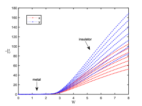
(a)

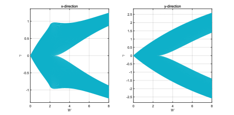
(b)

Figure S10: (a) Inverse normalized localization length $L_{\perp}/\xi_{\mu}$ along $x$ ($\mu=x$ and $L_{\perp}=L_{y}$ : red) and $y$ ($\mu=y$ and $L_{\perp}=L_{x}$: blue) as a function of disorder strength $W$ at $t_{x}=t_{y}=t$. The system size $L_{\perp}$ varies from $L_{\perp}=60$ to $L_{\perp}=120$. The figure suggests that the exponential localization lengths $\xi_{x}$ and $\xi_{y}$ along $x$ and $y$ diverge at the same critical disorder strength. (b) Distributions of the LEs of zero-energy state of $h$ along $x$ and $y$ as a function of the disorder strength $W$ at $t_{x}=t_{y}=t$.

References

Wen [2004]X.-G. Wen, Quantum Field Theory of Many-body Systems: From the Origin of Sound to an Origin of Light and Electrons (Oxford University Press, 2004).
Chiu et al. [2016]C.-K. Chiu, J. C. Y. Teo, A. P. Schnyder, and S. Ryu, Classification of topological quantum matter with symmetries, Reviews of Modern Physics 88, 035005 (2016).
Pruisken [1987]A. M. M. Pruisken, Quasi particles in the theory of the integral quantum Hall effect: (II). Renormalization of the Hall conductance or instanton angle theta, Nuclear Physics B 290, 61 (1987).
Zhang et al. [1989]S. C. Zhang, T. H. Hansson, and S. Kivelson, Effective-Field-Theory Model for the Fractional Quantum Hall Effect, Physical Review Letters 62, 82 (1989).
Niemi and Semenoff [1983]A. J. Niemi and G. W. Semenoff, Axial-Anomaly-Induced Fermion Fractionization and Effective Gauge-Theory Actions in Odd-Dimensional Space-Times, Physical Review Letters 51, 2077 (1983).
Wen and Zee [1992]X. G. Wen and A. Zee, Classification of Abelian quantum Hall states and matrix formulation of topological fluids, Physical Review B 46, 2290 (1992).
Lopez and Fradkin [1991]A. Lopez and E. Fradkin, Fractional quantum Hall effect and Chern-Simons gauge theories, Physical Review B 44, 5246 (1991).
Haldane [1983]F. D. M. Haldane, Nonlinear Field Theory of Large-Spin Heisenberg Antiferromagnets: Semiclassically Quantized Solitons of the One-Dimensional Easy-Axis Néel State, Physical Review Letters 50, 1153 (1983).
Affleck and Haldane [1987]I. Affleck and F. D. M. Haldane, Critical theory of quantum spin chains, Phys. Rev. B 36, 5291 (1987).
Altland et al. [2014]A. Altland, D. Bagrets, L. Fritz, A. Kamenev, and H. Schmiedt, Quantum Criticality of Quasi-One-Dimensional Topological Anderson Insulators, Physical Review Letters 112, 206602 (2014).
Altland et al. [2015]A. Altland, D. Bagrets, and A. Kamenev, Topology versus Anderson localization: Nonperturbative solutions in one dimension, Physical Review B 91, 085429 (2015).
Altland and Merkt [2001]A. Altland and R. Merkt, Spectral and transport properties of quantum wires with bond disorder, Nuclear Physics B 607, 511 (2001).
Haldane [1988]F. D. M. Haldane, O(3) nonlinear model and the topological distinction between integer- and half-integer-spin antiferromagnets in two dimensions, Phys. Rev. Lett. 61, 1029 (1988).
Read and Sachdev [1989]N. Read and S. Sachdev, Valence-bond and spin-peierls ground states of low-dimensional quantum antiferromagnets, Phys. Rev. Lett. 62, 1694 (1989).
Read and Sachdev [1990]N. Read and S. Sachdev, Spin-peierls, valence-bond solid, and néel ground states of low-dimensional quantum antiferromagnets, Phys. Rev. B 42, 4568 (1990).
Senthil et al. [2004]T. Senthil, A. Vishwanath, L. Balents, S. Sachdev, and M. P. A. Fisher, Deconfined quantum critical points, Science 303, 1490 (2004).
König et al. [2012]E. J. König, P. M. Ostrovsky, I. V. Protopopov, and A. D. Mirlin, Metal-insulator transition in two-dimensional random fermion systems of chiral symmetry classes, Physical Review B 85, 195130 (2012).
Luo et al. [2020]X. Luo, B. Xu, T. Ohtsuki, and R. Shindou, Critical behavior of Anderson transitions in three-dimensional orthogonal classes with particle-hole symmetries, Physical Review B 101, 020202 (2020).
Wang et al. [2021]T. Wang, T. Ohtsuki, and R. Shindou, Universality classes of the anderson transition in the three-dimensional symmetry classes aiii, bdi, c, d, and ci, Phys. Rev. B 104, 014206 (2021).
Karcher et al. [2023a]J. F. Karcher, I. A. Gruzberg, and A. D. Mirlin, Metal-insulator transition in a two-dimensional system of chiral unitary class, Phys. Rev. B 107, L020201 (2023a).
Karcher et al. [2023b]J. F. Karcher, I. A. Gruzberg, and A. D. Mirlin, Generalized multifractality in two-dimensional disordered systems of chiral symmetry classes, Phys. Rev. B 107, 104202 (2023b).
Xiao et al. [2023]Z. Xiao, K. Kawabata, X. Luo, T. Ohtsuki, and R. Shindou, Anisotropic Topological Anderson Transitions in Chiral Symmetry Classes, Physical Review Letters 131, 056301 (2023).
Feinberg and Zee [1997]J. Feinberg and A. Zee, Non-hermitian random matrix theory: Method of hermitian reduction, Nuclear Physics B 504, 579 (1997).
Luo et al. [2022]X. Luo, Z. Xiao, K. Kawabata, T. Ohtsuki, and R. Shindou, Unifying the Anderson transitions in Hermitian and non-Hermitian systems, Physical Review Research 4, L022035 (2022).
Altland and Zirnbauer [1997]A. Altland and M. R. Zirnbauer, Nonstandard symmetry classes in mesoscopic normal-superconducting hybrid structures, Physical Review B 55, 1142 (1997).
[36]Supplemental materials include NLSM in chiral symmetry classes, vortex excitations in the NLSM, quantum interference effect due to the weak topological term, dual theory of the NLSM, renormalization group (RG) analysis of the dual theory, details of RG phase diagrams for and cases, and details of the transfer matrix analyses of the 2D tight-binding model.
Li [2022]C.-A. Li, Topological States in Two-Dimensional Su-Schrieffer-Heeger Models, Frontiers in Physics 10 (2022).
Mondragon-Shem et al. [2014]I. Mondragon-Shem, T. L. Hughes, J. Song, and E. Prodan, Topological Criticality in the Chiral-Symmetric AIII Class at Strong Disorder, Physical Review Letters 113, 046802 (2014).
Claes and Hughes [2020]J. Claes and T. L. Hughes, Disorder driven phase transitions in weak aiii topological insulators, Phys. Rev. B 101, 224201 (2020).
Slevin and Ohtsuki [2014]K. Slevin and T. Ohtsuki, Critical exponent for the Anderson transition in the three-dimensional orthogonal universality class, New Journal of Physics 16, 015012 (2014).
Luo et al. [2021]X. Luo, T. Ohtsuki, and R. Shindou, Transfer matrix study of the Anderson transition in non-Hermitian systems, Physical Review B 104, 104203 (2021).
Karcher et al. [2023c]J. F. Karcher, I. A. Gruzberg, and A. D. Mirlin, Metal-insulator transition in a two-dimensional system of chiral unitary class, Physical Review B 107, L020201 (2023c).
Fradkin et al. [2010]E. Fradkin, S. A. Kivelson, M. J. Lawler, J. P. Eisenstein, and A. P. Mackenzie, Nematic Fermi Fluids in Condensed Matter Physics, Annu. Rev. Condens. Matter Phys. 1, 153 (2010).
Chayes et al. [1986]J. T. Chayes, L. Chayes, D. S. Fisher, and T. Spencer, Finite-size scaling and correlation lengths for disordered systems, Phys. Rev. Lett. 57, 2999 (1986).
Lin et al. [2021]L. Lin, Y. Ke, and C. Lee, Real-space representation of the winding number for a one-dimensional chiral-symmetric topological insulator, Physical Review B 103, 224208 (2021).